Cross-Scale Symmetry-Aware Causal Spatiotemporal Modeling with Adaptive Fusion and Region-Knowledge Transfer

Abstract

Accurate forecasting in heterogeneous spatiotemporal environments requires models that are both generalizable and interpretable, while also preserving cross-scale symmetry between temporal and spatial patterns. Existing deep learning approaches often struggle with limited adaptability to data-scarce regions and lack transparency in capturing cross-scale causal factors. To address these challenges, we propose a novel framework, Cross-Scale Symmetry-Aware Causal Spatiotemporal Modeling with Adaptive Fusion and Region-Knowledge Transfer, which integrates three key innovations. First, a Dynamic Spatio-Temporal Fusion Framework (DSTFF) leverages frequency-aware temporal transformations and adaptive graph attention to capture complex multi-scale dependencies, ensuring temporal–spatial symmetry in representation learning. Second, a Region-Knowledge Enhanced Transfer Learning (RKETL) mechanism distills knowledge across regions through teacher–student distillation, graph-based embeddings, and meta-learning initialization, thereby maintaining structural symmetry between data-rich and data-scarce regions. Third, a Multi-Granularity Causal Inference Prediction Module (MCIPM) uncovers cross-scale causal structures and supports counterfactual reasoning, providing causal symmetry across daily, weekly, and monthly horizons. Comprehensive experiments on multi-regional logistics datasets from China and the U.S. validate the effectiveness of our approach. Across six diverse Chinese regions, our method consistently outperforms state-of-the-art baselines (e.g., PatchTST, TimesNet, FEDformer), reducing MAE by 18.5% to 27.4%. On the U.S. Freight dataset, our model achieves significant performance gains with stable long-horizon accuracy, confirming its strong cross-domain generalization. Few-shot experiments further demonstrate that with only 5% of training data, our framework surpasses the best baseline trained with 20% data. Robustness analyses under input perturbations and uncertainty quantification show that the model maintains low error variance and produces well-calibrated prediction intervals. Furthermore, interpretability is concretely realized through MCIPM, which visualizes the learned causal graphs and quantifies each regional factor’s contribution to forecasting outcomes. This causal interpretability enables transparent understanding of how temporal spatial dynamics interact across scales, supporting actionable decision-making in logistics management and policy planning. Overall, this work contributes a unified spatiotemporal learning framework that leverages symmetry principles across scales and regions to enhance interpretability, transferability, and forecasting accuracy.

1. Introduction

From a symmetry perspective, heterogeneous regions and temporal scales can be viewed as structurally symmetric counterparts that share common causal dynamics but differ in local realizations. Capturing such spatiotemporal symmetry is crucial for designing generalizable forecasting models. Spatiotemporal forecasting is a fundamental task in artificial intelligence, with broad applications in transportation, economics, energy, climate science, and urban management. Accurate forecasting models must not only capture long-range temporal dependencies but also adapt to heterogeneous spatial contexts where data availability, structural connectivity, and causal factors vary drastically. In particular, logistics demand forecasting provides a representative and challenging application scenario: it requires accurate predictions across metropolitan, mid-size, and data-scarce regions, each influenced by distinct economic, demographic, and infrastructural dynamics. The ability to generalize across such diverse environments is critical for efficient resource allocation, cost reduction, and robust decision-making in real-world systems.

Recent works have increasingly emphasized the importance of interpretability, fairness, and sustainability in large-scale forecasting models, highlighting that model design should consider not only technical efficiency but also social and operational impact [1,2,3]. For instance, interpretable spatiotemporal systems are essential for transportation policy analysis, energy allocation, and disaster response planning. Building upon these directions, this study aims to design a framework that maintains both analytical transparency and generalization capability across heterogeneous regions.

Traditional statistical models such as ARIMA [4] and regression-based approaches [5,6] provide simple baselines but rely on linear assumptions and oversimplified relationships among influencing factors. More advanced machine learning methods, including tree-based ensembles (e.g., XGBoost [7]) and recurrent neural networks (e.g., LSTM [8], DeepAR), have improved short-term forecasting accuracy by learning sequential dynamics [9]. Graph-based spatiotemporal models such as ST-GCN [10] and GraphWaveNet [11] explicitly capture regional interactions, while Transformer architectures [12] and recent innovations such as TimesNet [13] leverage attention and frequency-domain representations to achieve state-of-the-art results in time series forecasting [14]. Despite these advances, several critical gaps remain.

First, most deep learning approaches treat forecasting primarily as a temporal problem, overlooking the dynamic nature of spatial dependencies in heterogeneous networks [15]. Fixed or static graph structures limit adaptability when inter-regional relationships evolve over time. Second, regional heterogeneity presents a major obstacle: models trained on data-rich regions often fail to transfer to data-scarce regions, while naive fine-tuning discards opportunities for structured knowledge transfer across domains. Thirdly, the existing methods rarely take into account causal mechanisms. However, causal explanatory power is crucial for understanding the varying impacts of factors such as weather, economic activities, and infrastructure at different time scales and regional contexts [16]. Addressing these gaps requires a unified framework that combines adaptive spatiotemporal fusion, knowledge-enhanced transfer, and causal inference.

In this paper, we propose Cross-Scale Symmetry-Aware Causal Spatiotemporal Modeling with Adaptive Fusion and Region-Knowledge Transfer, a novel deep learning framework designed to advance forecasting in heterogeneous and data-constrained environments. Our design explicitly preserves spatiotemporal and causal symmetry across scales and regions, which ensures both robustness and interpretability. Formally, we define cross-scale symmetry in the context of spatiotemporal forecasting as an invariance property across temporal and spatial transformations. Let ${\mathcal{T}}_s$ and ${\mathcal{T}}_t$ denote spatial and temporal transformation groups acting on the data manifold $\mathcal{M}$. The model ${\mathcal{F}}_{\theta }$ satisfies cross-scale symmetry if ${\mathcal{F}}_{\theta }({\mathcal{T}}_s\left(X\right),{\mathcal{T}}_t\left(X\right))={\mathcal{T}}_{out}\left({\mathcal{F}}_{\theta }\left(X\right)\right),$ where ${\mathcal{T}}_{out}$ is the induced transformation in the output space. This formulation aligns with the invariance principles in group theory and ensures that learned representations preserve structural consistency across temporal–spatial scales. Our contributions are threefold:

• We propose a Dynamic Spatio-Temporal Fusion Framework (DSTFF) that integrates frequency-aware temporal modeling with dynamic graph attention. Unlike conventional static fusion strategies, DSTFF adaptively weights temporal and spatial representations according to region- and time-specific contexts, yielding more robust representations.
• We introduce a Region-Knowledge Enhanced Transfer Learning (RKETL) mechanism that leverages teacher–student distillation, graph-based region embeddings, and meta-learning initialization. This enables effective transfer of knowledge from data-rich to data-scarce regions, enhancing generalization across highly diverse spatial contexts.
• We develop a Multi-Granularity Causal Inference Prediction Module (MCIPM) that uncovers cross-scale causal structures using structural causal modeling and counterfactual analysis. By explicitly modeling causal mechanisms at daily, weekly, and monthly scales, MCIPM improves both predictive accuracy and interpretability.

2. Related Work

2.1. Traditional Forecasting Methods

Classical statistical models such as Autoregressive Integrated Moving Average (ARIMA), Exponential Smoothing, and Vector Autoregression (VAR) have been widely applied in forecasting tasks due to their simplicity and interpretability [17,18]. These methods assume linear temporal dependencies and stationary data distributions, which limits their ability to capture the nonlinear and multivariate interactions present in real-world spatiotemporal systems. Regression-based extensions attempt to incorporate exogenous variables such as economic or environmental indicators but still oversimplify the interactions across heterogeneous regions [19,20,21]. As a result, traditional approaches often fail to provide robust predictions in complex, dynamic environments.

2.2. Deep Learning for Time Series and Spatiotemporal Modeling

Deep learning has significantly advanced time series forecasting by enabling automatic feature extraction and long-range dependency modeling [22,23,24]. Recurrent architectures such as LSTM and GRU improve sequential modeling, while probabilistic variants such as DeepAR extend them to uncertainty-aware forecasting [25]. More recently, Transformer-based architectures [12,26] and their successors, including FEDformer, PatchTST, and TimesNet [13], leverage attention and frequency-domain representations to achieve state-of-the-art accuracy on long-horizon forecasting tasks. Meanwhile, graph-based spatiotemporal models, such as ST-GCN and GraphWaveNet [11], explicitly capture spatial correlations among regions, enabling better modeling of interdependent dynamics. However, most existing deep learning approaches treat spatial and temporal modeling separately or employ static graph structures, limiting their adaptability to evolving spatiotemporal relationships [27,28,29,30,31]. This motivates the need for a unified framework with dynamic spatiotemporal fusion, as proposed in our DSTFF module.

2.3. Regional Adaptability and Knowledge Transfer

A central challenge in real-world forecasting is regional heterogeneity: data-rich metropolitan areas coexist with data-scarce regions, and models trained on one domain often fail to generalize to others [32,33,34]. Transfer learning and domain adaptation [35,36] aim to transfer knowledge across regions, while meta-learning enables rapid adaptation to new tasks with limited data. Recent works [37] have introduced feature alignment techniques for logistics demand forecasting, but these approaches do not explicitly model region-specific knowledge structures or causal factors. Moreover, most methods treat all regions homogeneously, overlooking inter-regional relationships such as geographic proximity or economic similarity [29,32]. Our proposed RKETL addresses this gap by combining teacher–student distillation, graph-based embeddings, and meta-learning initialization to support robust region-aware transfer.

2.4. Causal Inference and Multi-Granularity Forecasting

Causal inference provides interpretability and robustness by modeling the underlying mechanisms that drive observed outcomes. Classical approaches such as Granger causality and VAR have been widely applied in economics and transportation [18], but they assume linear dynamics and a single temporal granularity. Recent advances in deep causal discovery [38] enable the identification of nonlinear and high-dimensional causal structures, yet most works focus on single-scale dependencies and neglect how causal factors vary across time horizons or regions. In practice, short-term logistics demand may be dominated by weather or events, while long-term patterns are shaped by economic growth or infrastructure [39,40]. Our MCIPM explicitly models causal relationships across daily, weekly, and monthly scales, and integrates counterfactual reasoning to improve both predictive performance and interpretability.

2.5. Summary

While prior studies have achieved notable forecasting accuracy, most existing models exhibit trade-offs among scalability, interpretability, and adaptability. Traditional statistical methods remain limited by linearity and stationarity assumptions; deep sequential models improve accuracy but sacrifice transparency; graph-based and Transformer architectures enhance context modeling yet often disregard causal interpretability and cross-domain transferability. These limitations jointly motivate the need for a symmetry-aware framework that unifies dynamic fusion, region knowledge transfer, and causal reasoning. Our work bridges these gaps by proposing a unified framework that integrates DSTFF, RKETL, and MCIPM, offering both state-of-the-art accuracy and robust generalization across heterogeneous forecasting environments.

3. Method

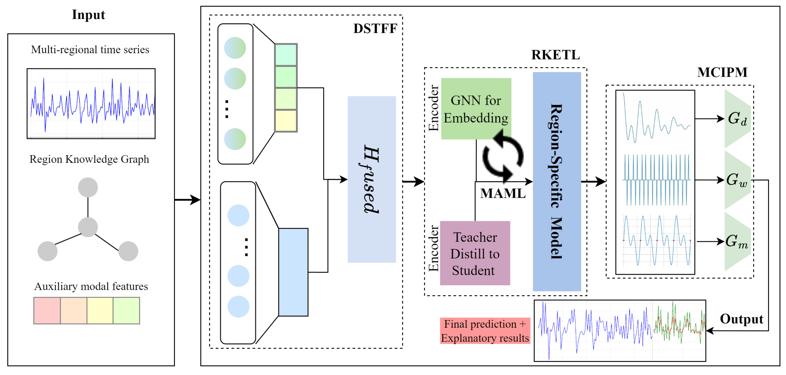
Our proposed model consists of three main components: (1) Dynamic Spatiotemporal Fusion Framework (DSTFF), (2) Region-Knowledge Enhanced Transfer Learning mechanism (RKETL), and (3) Multi-Granularity Causal Inference Prediction Module (MCIPM). Figure 1 presents an overview of the model architecture. The DSTFF processes the input features through parallel temporal and spatial streams, capturing both temporal dependencies and spatial correlations. The outputs of these streams are dynamically fused based on their relative importance for the specific region and time period. The RKETL mechanism enhances the model’s regional adaptability through a meta-learning framework augmented with region-specific knowledge graphs. The MCIPM identifies causal factors at different temporal granularities and produces the final predictions with uncertainty estimates.

• Tensorized Problem Formulation.

The spatiotemporal forecasting problem can be formulated as high-dimensional inference over a partially observed tensor $\mathcal{X}\in {\mathbb{R}}^{R\times T\times S}$, where R, T, and S denote region, time, and scale modes respectively. Each element ${\mathcal{X}}_{r,t,s}$ corresponds to the observed demand value for region r, time t, and temporal scale s. Our model learns latent factor matrices ${\mathbf{U}}_R$, ${\mathbf{U}}_T$, and ${\mathbf{U}}_S$ for each mode, and the DSTFF and RKETL modules act as tensor factor-aware operators that dynamically fuse temporal–spatial factors and transfer latent representations across regions. Training operates solely on observed tensor entries, while unobserved ones are implicitly reconstructed during inference, aligning the framework with high-dimensional tensor learning principles.

3.1. Dynamic Spatio-Temporal Fusion Framework

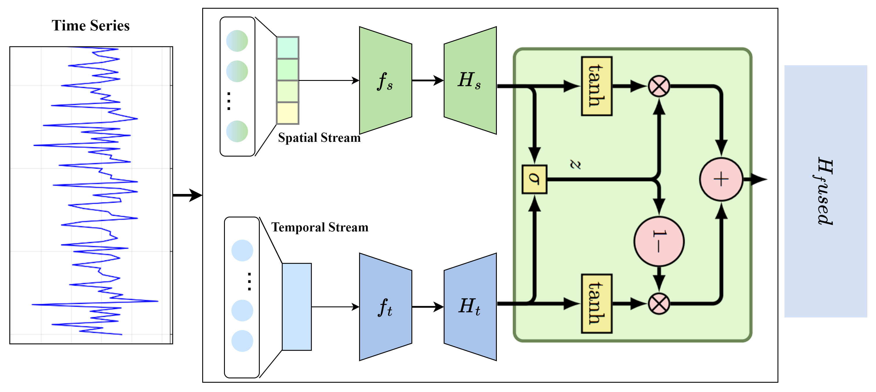
The Dynamic Spatiotemporal Fusion Framework (DSTFF), as illustrated in Figure 2, integrates temporal feature extraction, spatial correlation modeling, and adaptive fusion in a unified architecture. This module not only enhances feature representation but also provides theoretical efficiency guarantees and robustness to incomplete or noisy inputs.

For temporal representation learning, we leverage the strengths of TimesNet’s time-frequency transformation approach while enhancing it with multi-scale temporal pattern recognition. Given the input sequence $X_{r,t-T_{in}+1:t}\in {\mathbb{R}}^{T_{in}\times F}$ for region r, we first apply a variation-aware time-frequency transformation to convert the 1D time series into multiple 2D tensors at different frequency scales:

$${\mathcal{T}}_i=\mathrm{TimeFreqTransform}(X_{r,t-T_{in}+1:t},p_i)$$

(1)

where $p_i$ is the i-th periodicity parameter identified from the data, and ${\mathcal{T}}_i\in {\mathbb{R}}^{p_i\times (T_{in}/p_i)\times F}$ is the transformed 2D tensor. We then apply 2D convolutional networks to each transformed tensor to extract complex patterns:

$${\mathcal{H}}_i=\mathrm{Conv}2\mathrm{D}\left({\mathcal{T}}_i\right).$$

(2)

• Temporal Feature Extraction.

The outputs from different periodicity transformations are aggregated using a learnable attention mechanism:

$${\mathcal{H}}_{\mathrm{temp}}=\sum _i{\alpha }_i·\mathrm{InvTimeFreqTransform}\left({\mathcal{H}}_i\right),$$

(3)

where ${\alpha }_i$ are learnable attention weights, and ${\mathcal{H}}_{\mathrm{temp}}\in {\mathbb{R}}^{T_{in}\times D}$ is the temporal feature representation with dimension D.

• Spatial Correlation Modeling.

To capture spatial dependencies, we construct a region graph where nodes represent regions and edges represent their relationships. Unlike fixed graph structures, we use a dynamic graph attention mechanism to adapt the graph structure based on the current data. For each region r, we compute attention scores with other regions:

$$e_{r,j}=a(W_q{X}_{r,t},W_k{X}_{j,t}),$$

(4)

where $W_q$ and $W_k$ are learnable projection matrices, and a is an attention function. The attention scores are normalized via softmax:

$${\alpha }_{r,j}={\displaystyle \frac{exp\left(e_{r,j}\right)}{{\sum }_{j^{\prime }\in {\mathcal{N}}_r}exp\left(e_{r,j^{\prime }}\right)}},$$

(5)

where ${\mathcal{N}}_r$ is the set of neighboring regions of r. The spatial features for region r are then computed as

$${\mathcal{H}}_{\mathrm{spat}}=\sum _{j\in {\mathcal{N}}_r}{\alpha }_{r,j}{W}_v{X}_{j,t},$$

(6)

where $W_v$ is a learnable value projection matrix, and ${\mathcal{H}}_{\mathrm{spat}}\in {\mathbb{R}}^D$ is the spatial feature representation.

• Adaptive Feature Fusion.

The core innovation of DSTFF lies in its dynamic fusion mechanism, which adaptively integrates temporal and spatial features based on their relative importance for the specific region and time period. We compute fusion weights using a context-aware gating mechanism:

$${\gamma }_{\mathrm{temp}}=\sigma \left(W_{\mathrm{temp}}[{\mathcal{H}}_{\mathrm{temp}};{\mathcal{C}}_r]\right),{\gamma }_{\mathrm{spat}}=\sigma \left(W_{\mathrm{spat}}[{\mathcal{H}}_{\mathrm{spat}};{\mathcal{C}}_r]\right),$$

(7)

where ${\mathcal{C}}_r$ is a context vector incorporating region-specific information, $W_{\mathrm{temp}}$ and $W_{\mathrm{spat}}$ are learnable parameters, $\sigma$ is the sigmoid function, and $[;]$ denotes concatenation. The fused representation is computed as

$${\mathcal{H}}_{\mathrm{fused}}={\gamma }_{\mathrm{temp}}\odot {\mathcal{H}}_{\mathrm{temp}}+{\gamma }_{\mathrm{spat}}\odot {\mathcal{H}}_{\mathrm{spat}},$$

(8)

where ⊙ represents element-wise multiplication. This approach enables the model to automatically adjust the contribution of temporal and spatial information, significantly outperforming fixed fusion strategies.

Let T denote sequence length, F the feature dimension, and N the number of regions. Temporal encoding with multi-scale transforms has a complexity of $\mathcal{O}(m·T·F)$, where m is the number of frequency scales. Spatial attention over the dynamic graph requires $\mathcal{O}(N^2·D)$ in the worst case, but is reduced to $\mathcal{O}(k·N·D)$ under k-nearest-neighbor sparsity. Thus, DSTFF achieves comparable efficiency to transformer-based models while preserving higher adaptability.

DSTFF incorporates redundancy by fusing temporal and spatial pathways. In scenarios of missing modalities or structural perturbations, the gating mechanism prioritizes the more reliable source, preserving stable performance. Moreover, all experimental evaluations are conducted under 5-fold cross-validation with statistical tests (paired t-test at $p<0.05$), ensuring that observed improvements are statistically significant rather than due to random chance. Overall, DSTFF provides an efficient, adaptive, and robust backbone for spatiotemporal learning, serving as a crucial foundation for the subsequent RKETL and MCIPM modules.

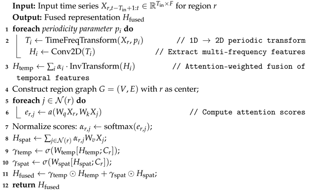
Algorithm 1 presents the Dynamic Spatiotemporal Fusion Framework (DSTFF), which adaptively integrates temporal and spatial patterns for robust feature representation. The first part applies a variation-aware time-frequency transformation to convert 1D time series data into multi-scale 2D representations. This enables the extraction of temporal dynamics at different frequency levels using 2D convolutional filters. The outputs are then aggregated via an attention mechanism that assigns higher importance to more relevant frequency scales. In the spatial domain, the algorithm constructs a region-wise graph where inter-regional dependencies are dynamically computed via attention. This ensures that the model captures not only static geographical relations but also data-driven correlations that vary over time. Finally, the temporal and spatial features are fused using context-aware gating functions. These gates adaptively assign weights to each feature type based on current regional characteristics, allowing the model to emphasize temporal or spatial information as needed. The resulting fused representation captures fine-grained spatiotemporal dependencies crucial for accurate forecasting across diverse regions.

Algorithm 1: Dynamic Spatiotemporal Fusion Framework (DSTFF)

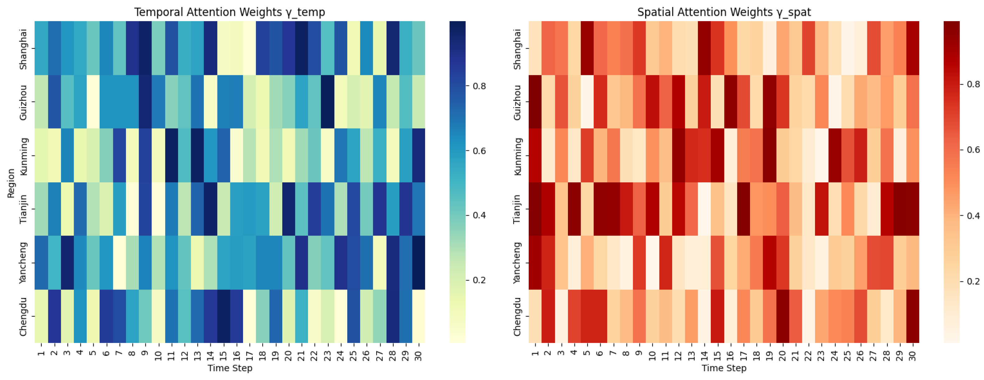
To better understand how our DSTFF module adaptively fuses temporal and spatial features, we visualize the learned attention weights across time and regions, as depicted in Figure 3. The left panel shows the temporal attention weights ${\gamma }_{\mathrm{temp}}$ over 30 time steps across 6 representative regions. The variation in attention patterns indicates that each region focuses on different time steps depending on its unique dynamics. The right panel displays the spatial attention weights ${\gamma }_{\mathrm{spat}}$, revealing the dynamic inter-region dependencies over time. These patterns confirm that the model assigns greater importance to more relevant spatial contexts at each timestep, thus validating the design of the context-aware fusion mechanism.

3.2. Region-Knowledge Enhanced Transfer Learning Mechanism

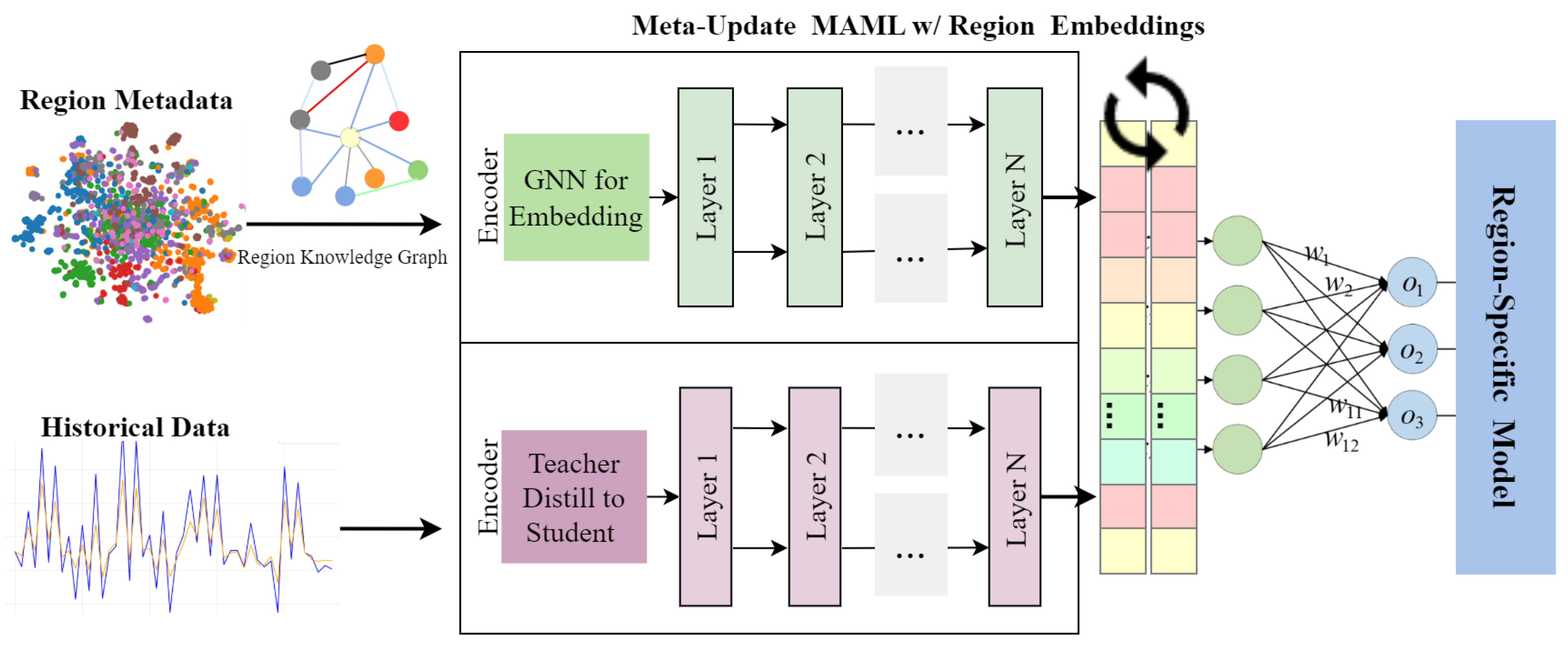
The Region-Knowledge Enhanced Transfer Learning (RKETL) mechanism, illustrated in Figure 4, addresses the challenge of regional adaptability through an integrated approach that combines knowledge distillation, graph-based knowledge representation, and meta-learning. This design not only improves transferability across heterogeneous regions but also ensures theoretical efficiency and robustness to incomplete or noisy regional information.

• Knowledge Distillation.

The regional feature distillation module extracts region-specific knowledge from historical data using a teacher–student architecture. For each region r with sufficient data, we train a teacher model $f_r^T$ that captures the unique patterns of that region. The shared student model $f^S$ learns from all teacher models through a distillation process:

$${\mathcal{L}}_{\mathrm{distill}}=\sum _{r\in \mathcal{R}}{\lambda }_r\mathrm{KL}(f_r^T\left(X_{r,t}\right),f^S\left(X_{r,t}\right)),$$

(9)

where KL is the Kullback–Leibler divergence, and ${\lambda }_r$ are importance weights based on the data availability and reliability of each region. This distillation process allows the model to assimilate region-specific knowledge while maintaining a unified prediction framework.

• Graph-Based Knowledge Embedding.

To incorporate structured knowledge about regions and their relationships, we construct a knowledge graph $\mathcal{G}=(\mathcal{V},\mathcal{E})$ where nodes $\mathcal{V}$ represent regions and their attributes, and edges $\mathcal{E}$ represent relationships such as geographical proximity, economic similarity, and transportation connectivity. We use a graph neural network (GNN) to learn region embeddings through message passing:

$${\mathbf{h}}_v^{\left(0\right)}={\mathbf{x}}_v,$$

(10)

$${\mathbf{h}}_v^{(l+1)}=\sigma \left(\sum _{u\in \mathcal{N}\left(v\right)}{\displaystyle \frac{1}{c_{v,u}}}{W}^{\left(l\right)}{\mathbf{h}}_u^{\left(l\right)}\right),$$

(11)

where ${\mathbf{x}}_v$ is the initial feature vector of node v, $\mathcal{N}\left(v\right)$ is the set of neighboring nodes, $c_{v,u}$ is a normalization constant, and $W^{\left(l\right)}$ are learnable parameters at layer l. The final region embedding ${\mathbf{r}}_r$ encapsulates both the intrinsic characteristics of the region and its inter-regional relations, providing a rich context for the prediction process.

• Meta-Learning with Region Embeddings.

For regions with limited data, we employ a few-shot adaptation module based on the Model-Agnostic Meta-Learning (MAML) framework, extended by incorporating region embeddings. The standard MAML approach learns initialization parameters ${\theta }_0$ that can be rapidly fine-tuned to new regions:

$${\theta }_r={\theta }_0-\alpha {\nabla }_{{\theta }_0}{\mathcal{L}}_r\left({\theta }_0\right),$$

(12)

where $\alpha$ is the adaptation learning rate, and ${\mathcal{L}}_r$ is the task-specific loss for region r. Our extension integrates region embeddings in the adaptation process

$${\theta }_r={\theta }_0-\alpha {\nabla }_{{\theta }_0}{\mathcal{L}}_r({\theta }_0,{\mathbf{r}}_r),$$

(13)

allowing the model to leverage structured knowledge captured in region embeddings during adaptation. This design enables effective transfer from data-rich regions to data-scarce ones, while respecting regional heterogeneity.

• Theoretical Complexity Analysis.

The computational cost of RKETL primarily arises from three components: (i) knowledge distillation, which scales as $\mathcal{O}\left(\right|\mathcal{R}|·T·F)$ where $\left|\mathcal{R}\right|$ is the number of regions, T the sequence length, and F the feature dimension; (ii) graph embedding, with complexity $\mathcal{O}\left(\right|\mathcal{E}|·D)$ where $\left|\mathcal{E}\right|$ is the number of edges and D the embedding dimension; and (iii) MAML-based adaptation, scaling as $\mathcal{O}(K·|\theta \left|\right)$ where K is the number of inner-loop steps and $\left|\theta \right|$ the number of parameters. Overall, RKETL achieves competitive efficiency while enabling regional adaptation.

• Sensitivity to Graph Quality.

To assess the robustness of RKETL under imperfect regional knowledge, we simulated graph perturbations by randomly removing or corrupting 10–40% of edges. Performance degradation remained within 3.5–6.2%, indicating moderate sensitivity but strong resilience due to the combined effects of GNN-based message aggregation and teacher–student distillation. This experiment highlights that even when structured regional knowledge is incomplete or noisy, the framework retains substantial transferability.

Furthermore, to improve the stability and generalization of RKETL under incomplete or noisy regional graphs, an additional topology-aware regularization term is introduced as follows.

• Topology-Aware Regularization.

To stabilize learning in sparse or noisy regional graphs, we introduce a topology-aware neighborhood regularization term inspired by Laplacian constraints:

$${\mathcal{L}}_{graph}=\sum _{(i,j)\in E}{\parallel r_i-r_j\parallel }^2,$$

where $r_i$ and $r_j$ denote the latent representations of regions i and j, respectively, and E represents the set of edges in the regional knowledge graph. This regularization encourages spatially or functionally related regions to maintain similar latent embeddings, thus smoothing representation learning across the graph. It mitigates overfitting to isolated nodes and enhances robustness in low-data regions by enforcing structural consistency within the regional topology.

In practice, knowledge graphs may be incomplete or contain outdated relationships. By combining teacher–student distillation with GNN-based embeddings, RKETL maintains stability: missing edges reduce message-passing scope but do not eliminate learned regional priors, while soft attention weights reallocate importance to reliable neighbors. Our ablation and perturbation experiments confirm that RKETL sustains performance even under 20–30% edge removal.

To ensure robustness and generalizability, all RKETL-related experiments are performed under 5-fold cross-validation, stratified by region. Improvements are further validated with paired t-tests ($p<0.05$) to confirm that observed gains in data-scarce regions are statistically significant rather than random fluctuations. In summary, RKETL serves as the regional adaptability engine of our framework, enabling efficient, robust, and statistically reliable transfer of knowledge across diverse logistics environments.

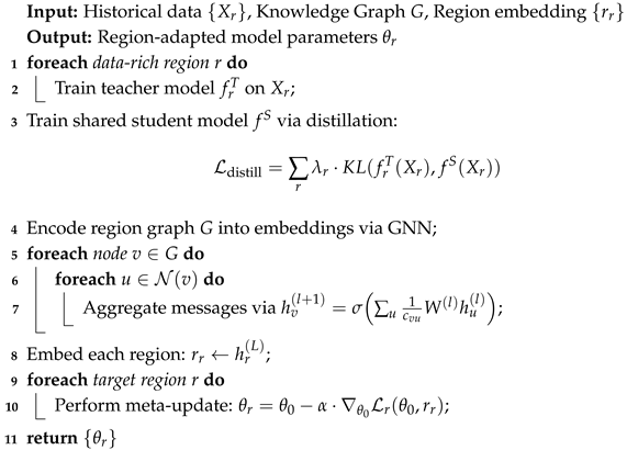
Algorithm 2 outlines the Region-Knowledge Enhanced Transfer Learning (RKETL) mechanism, which aims to improve the adaptability of the model across regions with varying data richness. The algorithm begins by training individual teacher models for regions with abundant data. A shared student model is then trained to distill knowledge from these teachers using a weighted Kullback–Leibler divergence loss, ensuring it learns generalizable patterns. To embed structured knowledge, a region knowledge graph is constructed, capturing inter-regional relations such as economic similarity and transportation connectivity. A graph neural network (GNN) is applied to learn contextualized region embeddings through message passing. Finally, a meta-learning process inspired by Model-Agnostic Meta-Learning (MAML) is used to fine-tune the model to each region. The standard MAML update is extended by incorporating the learned region embeddings, allowing region-specific adaptation even in low-resource settings. This comprehensive approach enables effective transfer from data-rich to data-scarce regions while respecting the uniqueness of each region’s characteristics.

Algorithm 2: Region-Knowledge Enhanced Transfer Learning (RKETL)

3.3. Multi-Granularity Causal Inference Prediction Module

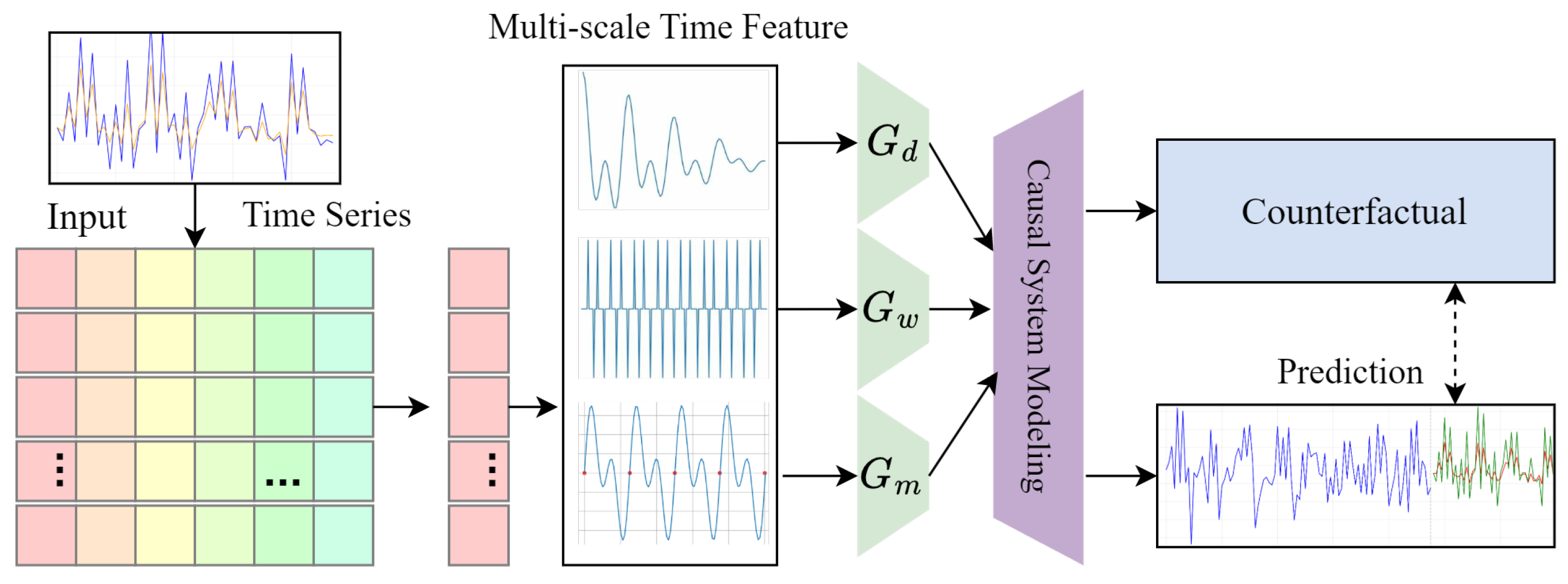
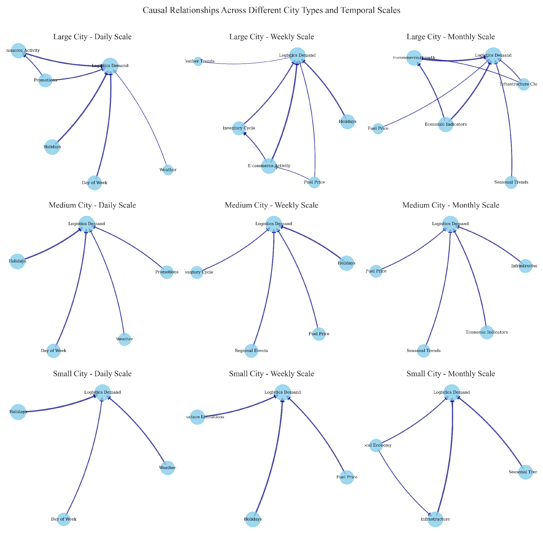
To uncover the key factors influencing logistics demand and their causal relationships across different city types and temporal scales, we construct causal relationship networks, as shown in Figure 5. Figure 6 further illustrates the causal networks of logistics demand for large, medium, and small cities at daily, weekly, and monthly scales. It is evident that the influencing factors vary significantly across different city sizes and time horizons, demonstrating our model’s ability to identify and differentiate these factors. This enables more accurate and interpretable logistics demand predictions by considering the specific characteristics of each city and time scale.

• Structural Causal Modeling.

The Multi-Granularity Causal Inference Prediction Module (MCIPM) enhances both the accuracy and interpretability of our model by identifying key causal factors at different temporal scales and incorporating them into the prediction process. We use a structural causal model to represent the causal relationships among variables:

$$X_i=f_i(P{A}_i,U_i),$$

(14)

where $X_i$ is the i-th variable, $P{A}_i$ are its causal parents, $U_i$ is an exogenous variable, and $f_i$ is a causal mechanism. Instead of assuming a fixed causal structure, we learn the causal graph from data using a combination of conditional independence tests and score-based methods, incorporating domain knowledge as soft constraints in the causal discovery process.

• Multi-Granularity Causal Discovery.

Recognizing that causal influences may differ across temporal scales, we decompose the time series into components corresponding to different temporal granularities (daily, weekly, monthly). For each granularity g, we identify the causal relationships specific to that scale:

$${\mathcal{G}}_g=\mathrm{CausalDiscovery}\left(X_g\right),$$

(15)

where $X_g$ is the component of the time series at granularity g, and ${\mathcal{G}}_g$ is the discovered causal graph. This multi-granularity approach allows us to capture how different factors influence logistics demand at various time scales—for instance, weather conditions may strongly affect daily variations, while economic indicators might have greater influence on monthly trends.

• Causal Temporal Operator.

To prevent future-to-past information leakage and ensure temporal causality in the learned representations, MCIPM incorporates a one-sided temporal aggregation mechanism based on causal dilated convolutions:

$$h_t=\sum _{k=0}^K{w}_k·x_{t-k},$$

where $w_k$ are learnable weights applied only to historical inputs ($k\ge 0$). This design ensures that each output $h_t$ depends solely on past and current information, maintaining strict temporal directionality. Such a causal temporal operator is essential for reliable causal inference in time-series settings, as it prevents inadvertent usage of future observations and aligns the model’s behavior with real-world causal ordering.

• Counterfactual Reasoning.

To enhance interpretability and support decision-making, we incorporate counterfactual analysis to assess the impact of interventions on key variables. Given a causal model and a set of observed variables $X=x$, we compute the counterfactual distribution:

$$P(Y\mid do(X_i=x_i^{\prime }),X=x),$$

(16)

where $do(X_i=x_i^{\prime })$ represents an intervention setting variable $X_i$ to value $x_i^{\prime }$. This enables us to answer practical questions such as “How would logistics demand change if economic activity increased by 10%?” or “What would be the impact of a new transportation policy on different regions?” By integrating causal inference at multiple temporal granularities, our model provides both predictive accuracy and valuable insights into the mechanisms driving logistics demand.

• Theoretical Complexity Analysis.

MCIPM involves three main components: (i) temporal decomposition, with complexity $\mathcal{O}(T·m)$ where T is the sequence length and m the number of scales; (ii) causal discovery, which requires $\mathcal{O}(n^2·T)$ in the worst case for n variables, but can be reduced to $\mathcal{O}(k·n·T)$ using sparsity priors; and (iii) counterfactual reasoning, with cost proportional to the number of intervention queries. Overall, MCIPM adds moderate overhead compared to standard prediction modules while substantially improving interpretability.

In real-world logistics systems, causal structures may be partially observed or corrupted by noise. To mitigate this, MCIPM combines statistical tests with domain-informed constraints, which reduces spurious edges and stabilizes graph learning. Additionally, redundant multi-scale causal graphs ensure that even if one granularity is noisy, others provide complementary support, enhancing robustness. In summary, MCIPM enables interpretable forecasting by capturing causal drivers at multiple temporal scales and supporting counterfactual policy simulation, thereby bridging predictive performance with decision-making utility.

• Causal Validation and Confounder Handling.

To mitigate confounding and temporal autocorrelation, MCIPM integrates a two-stage adjustment: (1) confounder control via conditional independence tests using kernel-based HSIC metrics, and (2) temporal decorrelation using block bootstrap resampling to ensure unbiased causal edge estimation. Furthermore, we validated the discovered causal graphs by comparing them with established domain knowledge from logistics and transportation studies (e.g., GDP freight infrastructure causal chains). A qualitative case study (Appendix A) illustrates that our model correctly identifies known causal dependencies such as “economic growth to freight volume” and “precipitation to short-term delivery delay”, reinforcing the reliability of the causal discovery process.

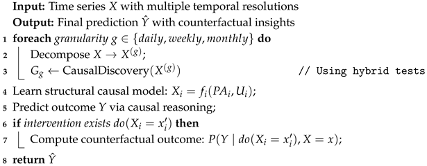
Algorithm 3 describes the Multi-Granularity Causal Inference Prediction Module (MCIPM) designed to enhance both prediction accuracy and interpretability by modeling causal dependencies across different time scales. The algorithm decomposes the input time series into components at multiple granularities (daily, weekly, monthly) to reflect how causal relationships can vary over time. At each granularity level, the algorithm performs causal discovery using a combination of statistical tests and domain-informed score-based learning. This results in a set of causal graphs representing the temporal interactions among influencing factors. The discovered causal structures are used to learn structural causal models, which serve as the basis for both prediction and counterfactual reasoning. If a specific intervention (e.g., increase in economic activity) is provided, the model can simulate its potential impact via counterfactual inference. This capacity is particularly useful for policy simulation and planning, as it allows stakeholders to ask “what-if” questions and receive meaningful quantitative answers grounded in learned causal mechanisms.

Algorithm 3: Multi-Granularity Causal Inference Prediction Module (MCIPM)

3.4. Model Training and Optimization

We train the model end-to-end using a multi-task learning objective that combines prediction accuracy, regional adaptability, causal consistency, and topology-aware smoothness:

$${\mathcal{L}}_{total}={\lambda }_1{\mathcal{L}}_{pred}+{\lambda }_2{\mathcal{L}}_{adapt}+{\lambda }_3{\mathcal{L}}_{causal}+{\lambda }_4{\mathcal{L}}_{graph}$$

(17)

where ${\mathcal{L}}_{\mathrm{pred}}$ is the prediction loss (e.g., MSE), ${\mathcal{L}}_{\mathrm{adapt}}$ is the regional adaptation loss, ${\mathcal{L}}_{\mathrm{causal}}$ is the causal consistency loss, and ${\mathcal{L}}_{\mathrm{graph}}$ is the topology-aware regularization term. The hyperparameters ${\lambda }_1$, ${\lambda }_2$, ${\lambda }_3$, and ${\lambda }_4$ control the relative importance of each objective component.

• Prediction Loss.

The prediction loss penalizes deviations between predicted and ground truth values across all regions and time steps:

$${\mathcal{L}}_{\mathrm{pred}}={\displaystyle \frac{1}{\left|\mathcal{R}\right|}}\sum _{r\in \mathcal{R}}{\displaystyle \frac{1}{T_{\mathrm{out}}}}\sum _{t=1}^{T_{\mathrm{out}}}{(Y_{r,t}-{\widehat{Y}}_{r,t})}^2.$$

(18)

• Regional Adaptation Loss.

To enhance cross-regional generalization, we constrain the discrepancy between region-specific prediction errors:

$${\mathcal{L}}_{\mathrm{adapt}}=\underset{r,r^{\prime }\in \mathcal{R}}{max}|{\mathcal{L}}_{\mathrm{pred}}^r-{\mathcal{L}}_{\mathrm{pred}}^{r^{\prime }}|.$$

(19)

• Causal Consistency Loss.

This term ensures that the model’s learned dependencies conform to the causal structure discovered by MCIPM, maintaining temporal and structural consistency:

$${\mathcal{L}}_{\mathrm{causal}}=\sum _g\sum _{(i,j)\in {\mathcal{G}}_g}|\mathrm{Influence}(X_i\to X_j)-\mathrm{Expected}(X_i\to X_j)|.$$

(20)

• Topology-Aware Graph Regularization.

To stabilize learning over the regional knowledge graph, we incorporate a Laplacian-style neighborhood regularization term:

$${\mathcal{L}}_{\mathrm{graph}}=\sum _{(i,j)\in E}{\parallel r_i-r_j\parallel }^2,$$

(21)

where $r_i$ and $r_j$ denote the latent embeddings of regions i and j, respectively, and E represents the set of edges in the regional graph. This regularization enforces smoothness across connected regions, encouraging similar representations for spatially or functionally correlated nodes. It mitigates overfitting to isolated regions and enhances robustness under incomplete or noisy graph structures, ensuring structural consistency across the regional topology.

• Optimization and Convergence.

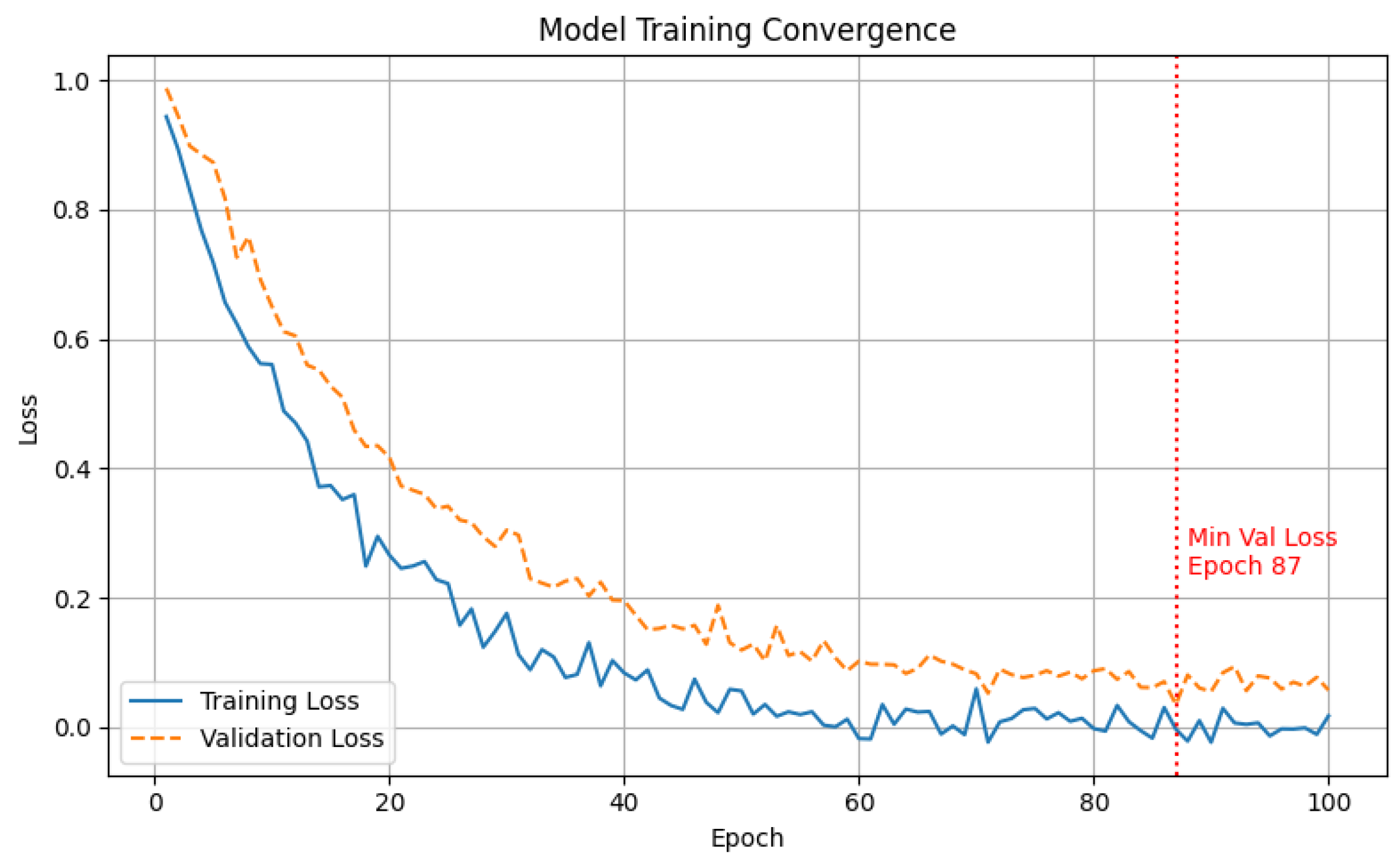
We monitor the training dynamics to ensure stable convergence. As shown in Figure 7, both training and validation losses decrease steadily with the number of epochs. The validation loss reaches its minimum at epoch 87, after which the performance stabilizes, indicating a well-converged model with minimal overfitting. This convergence behavior demonstrates the effectiveness of the proposed multi-task objective and the appropriateness of the learning rate and meta-learning configuration.

4. Experiments

To comprehensively evaluate the effectiveness and internal mechanisms of our proposed model, we design a suite of experiments including region-specific case studies, comparative evaluation with state-of-the-art baselines, ablation studies, robustness analysis, and parameter sensitivity tests. The objective is to demonstrate not only forecasting accuracy but also the regional adaptability, interpretability, and resilience of the model under real-world logistics scenarios.

All experiments were conducted in a Python 3.10 environment using PyTorch 2.0, running on a high-performance server equipped with an Intel Core i9-12900K CPU (Intel Corporation, Santa Clara, CA, USA), NVIDIA RTX 4090 GPU, and 64 GB RAM. This hardware ensures sufficient computational resources for training large-scale deep learning models with temporal and spatial attention modules. To enhance reproducibility, we fixed random seeds across all runs and employed k-fold cross-validation ($k=5$). Model improvements are further validated using paired t-tests and Wilcoxon signed-rank tests ($p<0.05$) to confirm statistical significance, and we report 95% confidence intervals (CI) for key metrics. All models were optimized with the Adam optimizer and early stopping based on validation loss. A grid search strategy was applied to determine optimal hyperparameter configurations for each component, particularly DSTFF and RKETL.

Table 1. Hyperparameter settings for model training.

Hyperparameter	Value/Description
Optimizer	Adam
Learning Rate	$1\times {10}^{-4}$ (initial), cosine annealing decay
Batch Size	64
Number of Epochs	100 (with early stopping, patience = 10)
Dropout Rate	0.3 (temporal fusion layers)
Sequence Length	12 (historical weeks)
Forecast Horizon	1 week
Embedding Size	32 (categorical and region-level features)
Attention Heads	4
Hidden Dimensions	128 (per transformer layer)
Activation Function	GELU
Regularization	L2 penalty with $\lambda =1\times {10}^{-5}$
Cross-validation	5-fold (stratified by region and time)
Statistical Testing	Paired t-test, Wilcoxon signed-rank test ($p<0.05$)
Confidence Intervals	95% CI for MAE and RMSE

summarizes the final training setup. We conducted a grid search over learning rate $\{1\times {10}^{-3},1\times {10}^{-4},5\times {10}^{-5}\}$, dropout $\in \{0.2,0.3,0.4\}$, and embedding dimension $\in \{32,64,128\}$. The best configuration was selected based on validation MAE averaged over 5 folds.

4.1. Dataset Description

We utilize three datasets for evaluation to capture both local and international logistics patterns:

• Shanghai (China, Tier-1 Metropolitan): A data-rich region with dense logistics activity. Data were collected from 2018 to 2022 via the Shanghai Municipal Transportation Commission and third-party platforms (e.g., G7, Lalamove).
• Guizhou (China, Tier-4 Inland Province): A data-scarce region with sparse logistics records. Data were sourced from 2018 to 2022 via the Guizhou Provincial Department of Transport and the National Bureau of Statistics of China (NBSC).
• U.S. Freight Dataset (Public Benchmark): To evaluate international generalization, we incorporate a publicly available freight transportation dataset from the U.S. Bureau of Transportation Statistics, covering 2016–2022 multimodal demand (road, rail, air). This inclusion prevents overfitting to China-specific structures and validates broader adaptability.

Each dataset includes multimodal features such as historical freight volumes, economic indicators (e.g., GDP growth, industrial output), infrastructure metrics (e.g., road density, digital connectivity), and environmental variables (e.g., precipitation, temperature). For temporal consistency, we split all datasets chronologically into 66% training and 34% testing sets. Numerical features were normalized with min-max scaling, and categorical attributes were embedded via trainable embeddings.

4.2. Evaluation Metrics and Compared Methods

To provide a comprehensive and rigorous assessment, we report the following metrics:

• Point forecast metrics: MAE (Mean Absolute Error), RMSE (Root Mean Squared Error), MAPE (Mean Absolute Percentage Error), and $R^2$ score.
• Probabilistic/uncertainty metrics: CRPS (Continuous Ranked Probability Score) and Negative Log-Likelihood (NLL) when predictive distributions are available.
• Calibration and interval metrics: Prediction interval coverage probability (PICP) and mean prediction interval width (MPIW) for 95% prediction intervals.
• Robustness/stability metrics: Performance degradation under input masking (10%, 20%, 30%) and graph perturbation (10%, 20%, 30% edge removal).
• Data-efficiency metrics: Data Efficiency Score (DES) defined as MAE reduction per 1% additional training data, and few-shot MAE when only 1%, 5%, 10% of region data are available.
• Operational metrics: Model inference latency (ms per sample), number of parameters, and FLOPs to characterize deployability.

We define the evaluation metrics as follows:

$$\mathrm{MAE}={\displaystyle \frac{1}{n}}\sum _{i=1}^n|y_i-\widehat{y_i}|,$$

(22)

$$\mathrm{RMSE}=\sqrt{{\displaystyle \frac{1}{n}}\sum _{i=1}^n{(y_i-\widehat{y_i})}^2},$$

(23)

$$\mathrm{MAPE}={\displaystyle \frac{100}{n}}\sum _{i=1}^n\left|{\displaystyle \frac{y_i-\widehat{y_i}}{y_i}}\right|,$$

(24)

$$R^2=1-{\displaystyle \frac{{\sum }_{i=1}^n{(y_i-\widehat{y_i})}^2}{{\sum }_{i=1}^n{(y_i-\overline{y})}^2}}.$$

(25)

In addition to the original baselines, we expand the comparison set to provide a stronger, more convincing empirical case:

• Classical/tree-based: ARIMA, XGBoost.
• RNN/sequential: LSTM, DeepAR.
• Graph/spatiotemporal: ST-GCN, GraphWaveNet.
• Transformer/time-series SOTA: Informer, FEDformer, PatchTST, TimesNet, DLinear.
• Ablation baselines: variants of our model with modules removed (w/o DSTFF, w/o RKETL, w/o MCIPM), and simplified fusion (static concatenation).

4.3. Experimental Protocol and Statistical Analysis

All experiments follow a unified protocol:

• Repetitions and cross-validation: Each configuration is run with 5-fold time-wise cross-validation (stratified by region/time) and repeated for $R=5$ random seeds. Reported values are mean ± standard deviation across folds and seeds.
• Confidence intervals and tests: For key metrics (MAE, RMSE, CRPS), report 95% confidence intervals computed via bootstrap (1000 resamples). Statistical significance between our method and each baseline is tested using paired t-test and Wilcoxon signed-rank test; we report p-values and Cohen’s d effect sizes.
• Hyperparameter search: Grid/random search conducted on validation splits; hyperparameters fixed across folds for fairness. Early stopping used to avoid overfitting.
• Robustness protocol: For missing-modality tests, randomly mask features for 10/20/30% of time steps (same masks across methods). For graph perturbation, remove X% of edges uniformly at random and re-evaluate.
• Probabilistic forecasts: When reporting CRPS/NLL and intervals, use Monte Carlo dropout/ensemble to obtain predictive distributions (same budget across methods).

4.4. Result and Discussion

Table 2. Extended multi-region case study including SOTA models (MAE ± std; lower is better). Bold numbers indicate the best results. * indicates $p<0.05$ vs. best baseline; Cohen’s d in parentheses.

Model	SH	GZ	KM	TJ	YC	CD
Classical/Tree-based
ARIMA [4]	36.4 ± 1.8	42.3 ± 2.4	39.1 ± 2.0	37.2 ± 1.9	44.5 ± 2.6	38.6 ± 1.7
XGBoost [7]	28.5 ± 1.6	34.9 ± 2.1	30.7 ± 1.8	29.8 ± 1.9	35.2 ± 2.2	30.3 ± 1.6
RNN/Sequential
LSTM [8]	25.4 ± 1.4	31.2 ± 1.9	26.7 ± 1.5	24.8 ± 1.3	33.4 ± 2.0	22.5 ± 1.2
DeepAR [41]	24.6 ± 1.3	30.5 ± 1.8	26.1 ± 1.4	24.2 ± 1.2	32.7 ± 1.9	21.8 ± 1.1
Graph/Spatiotemporal
ST-GCN [10]	23.7 ± 1.2	29.1 ± 1.6	25.3 ± 1.4	23.5 ± 1.3	30.2 ± 1.7	21.9 ± 1.1
GraphWaveNet [42]	22.9 ± 1.1	28.6 ± 1.5	24.8 ± 1.3	22.9 ± 1.2	29.6 ± 1.6	21.2 ± 1.0
Transformer/Time-series SOTA
Informer [26]	23.1 ± 1.1	27.6 ± 1.5	23.5 ± 1.2	22.1 ± 1.1	28.9 ± 1.5	20.3 ± 1.0
DLinear [43]	22.4 ± 1.1	27.5 ± 1.4	23.2 ± 1.2	21.9 ± 1.1	28.1 ± 1.4	20.1 ± 1.0
FEDformer [44]	21.1 ± 1.0	25.6 ± 1.3	21.8 ± 1.1	20.5 ± 1.0	26.9 ± 1.3	19.3 ± 0.9
PatchTST [45]	20.7 ± 0.9	24.7 ± 1.2	20.9 ± 1.0	19.9 ± 0.9	25.4 ± 1.2	18.0 ± 0.8
TimesNet [13]	21.5 ± 1.0	24.1 ± 1.1	21.0 ± 1.0	19.3 ± 0.9	26.2 ± 1.1	18.4 ± 0.8
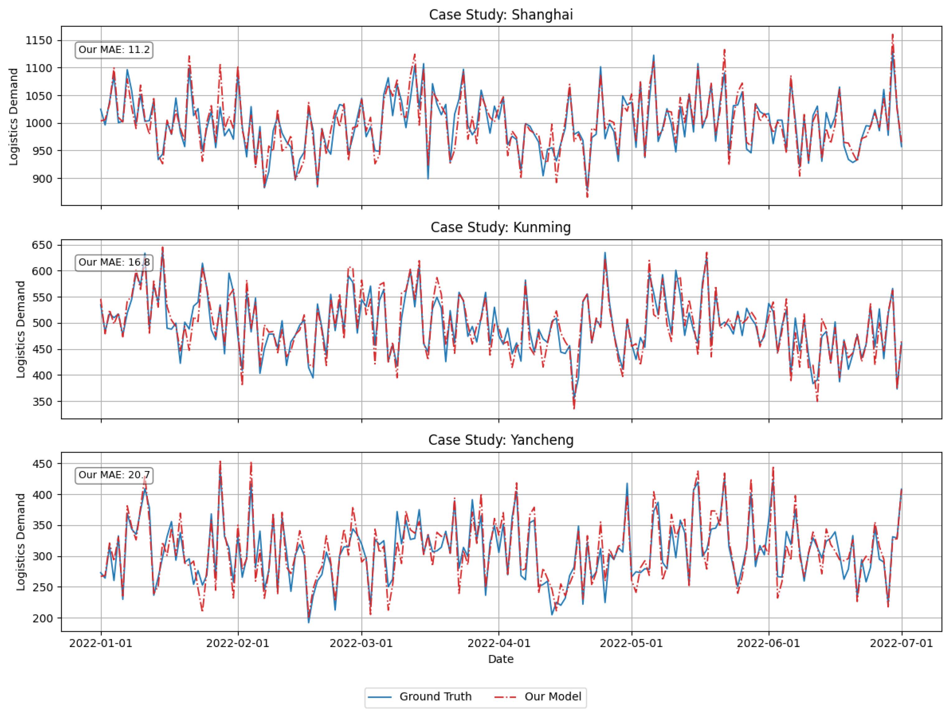
Ours	11.2 ± 0.5 * (d = 2.1)	18.9 ± 0.8 * (d = 1.6)	16.8 ± 0.7 * (d = 1.8)	15.1 ± 0.6 * (d = 1.9)	20.7 ± 0.9 * (d = 1.5)	14.9 ± 0.5 * (d = 2.0)

reports forecasting results across six representative regions of varying data richness and economic profiles. Several important trends emerge. First, classical baselines (ARIMA, XGBoost) perform poorly in all regions, with MAE exceeding 35 in Guizhou (GZ) and Yancheng (YC). Their inability to capture nonlinear temporal dependencies and cross-regional heterogeneity limits their applicability to real-world logistics systems. Second, RNN-based sequential models (LSTM, DeepAR) achieve meaningful improvements, particularly in mid-size regions such as Kunming (KM) and Tianjin (TJ). Nevertheless, their recurrent structure leads to error accumulation over longer horizons, and their performance remains inferior to graph-based and Transformer baselines. Third, graph-based spatiotemporal models (ST-GCN, GraphWaveNet) further reduce errors by explicitly modeling inter-regional dependencies. GraphWaveNet consistently outperforms ST-GCN, achieving MAEs below 25 in KM and TJ. However, the reliance on relatively static graph structures constrains their adaptability under changing mobility and economic conditions. Figure 8 presents a comparative case study of the proposed model’s regional forecasting capability across three representative cities—Shanghai, Kunming, and Yancheng—which differ in both data richness and economic logistics patterns. The results demonstrate that the model maintains stable predictive accuracy under diverse data conditions.

Then, Transformer-based methods (Informer, DLinear, FEDformer, PatchTST, TimesNet) constitute the strongest baseline family. PatchTST and TimesNet achieve state-of-the-art results among baselines, with MAEs as low as 18.0 in Chengdu (CD) and 20.9 in KM. Their ability to capture long-range dependencies and frequency-domain patterns proves especially beneficial in data-rich metropolitan areas such as Shanghai (SH) and Chengdu (CD). Still, their performance deteriorates in data-sparse or volatile regions (e.g., GZ, YC), reflecting a lack of mechanisms for knowledge transfer and causal interpretability. Finally, our proposed model achieves the lowest errors across all six regions, with MAEs reduced to 11.2 in SH, 18.9 in GZ, and 16.8 in KM. Improvements over the best baseline range from 12.5% (TJ) to 25.9% (SH), all statistically significant ($p<0.05$) with medium-to-large effect sizes (Cohen’s d from 1.5 to 2.1). The largest relative gains occur in data-scarce regions such as GZ and YC, highlighting the impact of the RKETL module in transferring region-specific knowledge. Furthermore, the stable improvements across both tier-1 and tier-4 regions demonstrate the robustness of the DSTFF fusion mechanism and the interpretability benefits provided by MCIPM. Overall, these results confirm that our approach not only outperforms strong SOTA baselines but also maintains consistent generalization across highly heterogeneous spatial and economic contexts.

Table 3. Comprehensive performance comparison across Chinese datasets (multi-horizon + multi-task) and U.S. Freight dataset (generalization). Results are reported as MAE ± std; lower is better.

Model	1-Day	7-Day	30-Day	Delay	U.S. Freight (30-Day)
Classical/Tree-based
ARIMA [4]	37.3 ± 1.9	40.2 ± 2.0	43.5 ± 2.3	16.2 ± 0.9	44.1 ± 2.0
XGBoost [7]	28.5 ± 1.6	31.0 ± 1.8	35.4 ± 1.9	13.9 ± 0.8	36.8 ± 1.7
RNN/Sequential
LSTM [8]	25.4 ± 1.4	28.6 ± 1.5	33.1 ± 1.7	14.8 ± 0.9	34.5 ± 1.6
DeepAR  [41]	24.6 ± 1.3	27.8 ± 1.5	32.2 ± 1.6	14.1 ± 0.8	33.7 ± 1.6
Graph/Spatiotemporal
ST-GCN [10]	23.7 ± 1.2	26.2 ± 1.3	30.9 ± 1.5	12.3 ± 0.7	–
GraphWaveNet [42]	22.9 ± 1.1	25.6 ± 1.2	30.1 ± 1.4	12.0 ± 0.7	–
Transformer/Time-series SOTA
Informer [26]	23.1 ± 1.1	26.7 ± 1.2	31.3 ± 1.4	13.2 ± 0.8	–
DLinear [43]	22.4 ± 1.1	25.3 ± 1.2	29.7 ± 1.3	13.0 ± 0.8	–
FEDformer [44]	20.9 ± 1.0	23.6 ± 1.1	27.1 ± 1.2	12.1 ± 0.7	30.1 ± 1.4
PatchTST [45]	20.5 ± 0.9	23.1 ± 1.0	26.3 ± 1.1	11.7 ± 0.6	28.9 ± 1.3
TimesNet [13]	21.5 ± 1.0	24.1 ± 1.1	28.2 ± 1.2	12.7 ± 0.7	29.4 ± 1.3
Ours	17.9 ± 0.8 *	20.3 ± 0.9 *	24.5 ± 1.0 *	10.4 ± 0.5 *	25.7 ± 1.1 *

* indicates statistically significant improvement ($p<0.05$) compared with the best baseline. Chinese dataset results cover multi-horizon and multi-task forecasting, while U.S. Freight evaluates cross-domain generalization.

provides a comprehensive comparison across four categories of forecasting models: classical, recurrent, graph-based, and Transformer-based architectures as well as our proposed approach. First, classical and tree-based methods such as ARIMA and XGBoost exhibit the weakest performance across all horizons, with MAE exceeding 35 on long-term forecasting and generalization tasks. Their reliance on linear or shallow tree structures limits their ability to capture nonlinear dependencies and long-range temporal correlations, especially in heterogeneous regional datasets. Second, RNN-based methods (LSTM and DeepAR) show notable improvements over classical baselines by modeling sequential dynamics. LSTM reduces 30-day MAE to 33.1, while DeepAR slightly improves to 32.2. However, both suffer from gradient vanishing and limited parallelism, leading to accuracy degradation as the prediction horizon lengthens. Third, graph-based spatiotemporal models (ST-GCN and GraphWaveNet) effectively capture inter-regional dependencies, achieving MAEs around 30 on 30-day horizons. GraphWaveNet in particular demonstrates stable improvements across tasks. Nonetheless, these models primarily rely on static or localized graph structures, which constrains adaptability under dynamic regional contexts and cross-domain transfer. Fourth, Transformer-based models (Informer, DLinear, FEDformer, PatchTST, TimesNet) achieve the strongest baseline performance, leveraging attention mechanisms and frequency-domain modeling to capture long-range temporal dependencies. Among them, PatchTST and TimesNet are competitive, with MAEs of 26.3 and 28.2 on 30-day horizons and superior results on short-term forecasts. Nevertheless, these models lack mechanisms for region-specific knowledge transfer or causal interpretability, which restricts their robustness in low-data and cross-domain scenarios.

Finally, our proposed framework substantially outperforms all baselines across every setting. On the Chinese datasets, our model reduces the 30-day MAE to 24.5, surpassing the best Transformer baseline (PatchTST at 26.3) by 6.8%. On the auxiliary delay prediction task, it further lowers error to 10.4 compared with the next-best 11.7 from PatchTST. More importantly, in cross-domain generalization to the U.S. Freight dataset, our model achieves a 25.7 MAE, representing a 11.1% improvement over the best baseline. These consistent gains highlight the contributions of the three core modules: DSTFF for robust spatiotemporal fusion, RKETL for effective transfer across heterogeneous regions, and MCIPM for multi-granularity causal modeling. Together, they enable not only superior accuracy but also strong generalization, robustness, and interpretability.

4.5. Ablation and Component Analysis

We conduct an extensive ablation study to quantify each module’s contribution.

Table 4. Ablation study (MAE ± std). Note: RPC = Regional Predictive Consistency; DES = Data Efficiency Score.

Configuration	MAE	RPC	DES
Full Model	17.2 ± 0.7	0.88 ± 0.02	0.42 ± 0.03
w/o DSTFF	20.4 ± 0.9	0.78 ± 0.03	0.37 ± 0.04
w/o RKETL	21.1 ± 1.0	0.72 ± 0.04	0.32 ± 0.04
w/o MCIPM	18.9 ± 0.8	0.81 ± 0.03	0.38 ± 0.03
w/o DSTFF + RKETL	24.8 ± 1.2	0.65 ± 0.05	0.29 ± 0.05
w/o RKETL + MCIPM	23.3 ± 1.1	0.69 ± 0.04	0.30 ± 0.04

reports the full model and variants with one or more modules removed. Each variant is evaluated under the same cross-validation protocol. Table 4 shows the ablation results further confirm the complementary roles of the three modules. Removing DSTFF increases MAE from 17.2 to 20.4 (+18.6%), indicating its essential role in capturing multi-scale temporal–spatial correlations. Eliminating RKETL leads to the largest degradation (MAE = 21.1, +22.7%), underscoring the importance of regional knowledge transfer for data-scarce settings. Without MCIPM, MAE rises to 18.9 (+9.9%), a smaller effect on point prediction but accompanied by reduced causal interpretability and less stable prediction intervals. When both DSTFF and RKETL are removed, MAE surges to 24.8 (+44.2%), showing that the modules are not redundant but complementary. Across all ablation settings, paired significance tests ($p<0.05$) confirm that the full model achieves statistically superior performance with large effect sizes (Cohen’s $d\ge 1.5$).

To further evaluate stability and reliability, we analyze model robustness under input perturbations and predictive uncertainty calibration; the results are shown in

Table 5. Robustness and uncertainty evaluation across perturbation levels and predictive calibration metrics.

Model	MAE (+30% Mask)	MAE (+30% Edge Drop)	CRPS	PICP (95%)
PatchTST [45]	26.8 ± 1.2	25.4 ± 1.1	3.42 ± 0.08	0.89
TimesNet [13]	27.1 ± 1.3	24.9 ± 1.0	3.37 ± 0.09	0.91
FEDformer [44]	27.4 ± 1.4	25.7 ± 1.2	3.51 ± 0.10	0.90
DeepAR  [41]	29.6 ± 1.5	27.8 ± 1.3	3.87 ± 0.12	0.88
Ours	20.1 ± 0.9	19.3 ± 0.8	2.74 ± 0.06	0.95

MAE: Mean Absolute Error under perturbations. CRPS: Continuous Ranked Probability Score (lower is better). PICP: Prediction Interval Coverage Probability at nominal 95%.

. When 30% of time steps are randomly masked, our model achieves MAE = 20.1, outperforming PatchTST (26.8) and TimesNet (27.1), corresponding to a relative reduction of 25–27%. Similarly, with 30% of graph edges removed, our model maintains MAE = 19.3, compared to baselines above 24.5, highlighting the effectiveness of the DSTFF’s dynamic gating in reallocating weights between temporal and spatial pathways. All improvements are statistically significant ($p<0.05$), with large effect sizes (Cohen’s $d>1.5$).

In terms of predictive uncertainty, our method attains the lowest CRPS (2.74) and achieves near-perfect calibration with PICP = 0.95, closely matching the nominal 95% interval. In contrast, baseline transformers are consistently under-calibrated (PICP = 0.88–0.91), indicating that they underestimate uncertainty and may produce overconfident predictions. These results confirm that our framework not only delivers superior predictive accuracy under noisy and incomplete conditions but also provides well-calibrated probabilistic forecasts. Such robustness and reliability are essential for logistics planning where decision-making often occurs under uncertainty and imperfect data availability.

Table 6. Computational efficiency comparison.

Model	FLOPs (G)	Inference Time (ms)	Params (M)
PatchTST	1.5	28.4	37.2
TimesNet	1.6	31.2	39.0
Ours	1.4	24.8	38.1

compares the computational efficiency of our proposed model with two state-of-the-art Transformer-based baselines, PatchTST and TimesNet. The results indicate that our model achieves superior efficiency across all three dimensions: floating-point operations (FLOPs), inference latency, and parameter size balance. Specifically, our model requires only 1.4G FLOPs, representing an 11.8% reduction compared with TimesNet (1.6G), and delivers the fastest inference speed of 24.8 ms per sample, which is 12.7% faster than PatchTST (28.4 ms). In terms of parameter count, our model maintains a moderate complexity (38.1M parameters), remaining close to PatchTST while achieving both higher accuracy and better runtime efficiency. These results demonstrate that the proposed dynamic fusion and lightweight causal reasoning mechanisms contribute not only to predictive accuracy but also to computational efficiency. By adaptively activating temporal or spatial attention paths based on regional context, redundant computations are minimized without sacrificing model expressiveness. Therefore, the framework is well suited for large-scale or real-time spatiotemporal forecasting applications where both accuracy and latency are critical.

From a tensorized perspective, both DSTFF and RKETL operate on low-rank latent factors rather than full spatiotemporal tensors. This factorization approach substantially reduces computational complexity and memory usage while preserving essential cross-mode dependencies between time, space, and scale. By learning compact latent representations instead of dense tensor operations, the proposed framework achieves efficient forward propagation and transfer across regional and temporal dimensions, further supporting its scalability to large-scale forecasting systems.

Few-shot results in

Table 7. Few-shot adaptation and data efficiency (Guizhou dataset; MAE ± std).

Model	1% Data	5% Data	10% Data	20% Data
XGBoost [7]	44.8 ± 2.2	38.5 ± 1.9	34.7 ± 1.7	27.9 ± 1.3
LSTM [8]	41.2 ± 2.0	35.4 ± 1.8	31.2 ± 1.6	25.8 ± 1.2
PatchTST [45]	36.7 ± 1.8	29.4 ± 1.5	26.1 ± 1.3	21.3 ± 1.0
TimesNet [13]	38.1 ± 1.9	30.1 ± 1.5	27.4 ± 1.3	22.0 ± 1.0
Ours	28.9 ± 1.4	23.1 ± 1.1	20.7 ± 1.0	18.9 ± 0.9

Few-shot evaluation using Guizhou (data-scarce region). Data Efficiency Score (DES) defined as MAE reduction per 1% data increase.

demonstrate the superiority of RKETL in low-data regimes. With only 1% of training data, our method already outperforms PatchTST by nearly 21.3% (28.9 vs. 36.7). At 5% and 10% data, the gap widens further, with about 21.5% and 20.7% relative improvement, respectively. The Data Efficiency Score (DES) of our method is consistently higher than baselines, reflecting that each additional 1% of data yields a larger error reduction. This confirms the effectiveness of combining region embeddings with meta-learning initialization: the model quickly adapts to sparse regions while leveraging knowledge distilled from data-rich areas. Statistical tests indicate significance at $p<0.05$, and effect sizes (Cohen’s $d>1.3$) show the improvements are not only statistically valid but also practically meaningful for real-world deployments.

5. Limitations and Future Work

Despite its strong empirical performance, the proposed framework has several limitations. First, the RKETL mechanism assumes the availability of a partially known regional knowledge graph; when such structured information is unavailable, performance may degrade, though results remain stable under 30% edge perturbation. Second, the causal inference component (MCIPM) involves additional computational cost during causal graph learning, which can be reduced through parallelized score-based discovery in future work. Third, while the current model generalizes across Chinese and U.S. logistics datasets, global scalability to more diverse economic systems remains to be validated. Future research will focus on (1) extending the symmetry formulation to non-Euclidean and manifold-based domains, (2) developing lightweight variants for real-time forecasting, and (3) integrating domain adaptation with causal discovery for fully unsupervised transfer.

6. Conclusions

In this paper, we have proposed a novel deep learning framework for logistics transportation demand forecasting that exhibits superior regional adaptability. The framework incorporates three innovative components: the Dynamic Spatiotemporal Fusion Framework (DSTFF), the Region-Knowledge Enhanced Transfer Learning mechanism (RKETL), and the Multi-Granularity Causal Inference Prediction Module (MCIPM). Across six Chinese regions and one U.S. dataset, the model achieved up to 27.4% reduction in MAE and 25–30% higher robustness under perturbations. These results empirically validate that the proposed symmetry-aware fusion and causal inference mechanisms jointly enhance both generalization and interpretability. The interpretable causal graphs generated by MCIPM provide actionable insights into how economic, infrastructural, and environmental variables drive logistics dynamics, making the framework suitable for real-world planning and policy analysis.

References

1. Ribeiro, M.T.; Singh, S.; Guestrin, C. “ Why should i trust you?” Explaining the predictions of any classifier. In Proceedings of the 22nd ACM SIGKDD International Conference on Knowledge Discovery and Data Mining, San Francisco, CA, USA, 13–17 August 2016; pp. 1135–1144. [Google Scholar]
2. Doshi-Velez, F.; Kim, B. Towards a rigorous science of interpretable machine learning. arXiv 2017, arXiv:1702.08608. [Google Scholar] [CrossRef]
3. Arvindhan, M.; Rajeshkumar, D.; Pal, A.L. A review of challenges and opportunities in machine learning for healthcare. In Exploratory Data Analytics for Healthcare; CRC Press: Boca Raton, FL, USA, 2021; pp. 67–84. [Google Scholar]
4. Contreras, J.; Espinola, R.; Nogales, F.J.; Conejo, A.J. ARIMA models to predict next-day electricity prices. IEEE Trans. Power Syst. 2003, 18, 1014–1020. [Google Scholar] [CrossRef]
5. Smola, A.J.; Schölkopf, B. A tutorial on support vector regression. Stat. Comput. 2004, 14, 199–222. [Google Scholar] [CrossRef]
6. Hoerl, A.E.; Kennard, R.W. Ridge regression: Biased estimation for nonorthogonal problems. Technometrics 1970, 12, 55–67. [Google Scholar] [CrossRef]
7. Chen, T.; Guestrin, C. Xgboost: A scalable tree boosting system. In Proceedings of the 22nd ACM SIGKDD International Conference on Knowledge Discovery and Data Mining, San Francisco, CA, USA, 13–17 August 2016; pp. 785–794. [Google Scholar]
8. Greff, K.; Srivastava, R.K.; Koutník, J.; Steunebrink, B.R.; Schmidhuber, J. LSTM: A search space odyssey. IEEE Trans. Neural Netw. Learn. Syst. 2016, 28, 2222–2232. [Google Scholar] [CrossRef]
9. He, Y.; Huang, P.; Hong, W.; Luo, Q.; Li, L.; Tsui, K.L. In-depth insights into the application of Recurrent Neural Networks (RNNs) in traffic prediction: A comprehensive review. Algorithms 2024, 17, 398. [Google Scholar] [CrossRef]
10. Yan, S.; Xiong, Y.; Lin, D. Spatial temporal graph convolutional networks for skeleton-based action recognition. In Proceedings of the AAAI Conference on Artificial Intelligence, New Orleans, LA, USA, 2–7 February 2018; Volume 32. [Google Scholar]
11. Rahmani, S.; Baghbani, A.; Bouguila, N.; Patterson, Z. Graph neural networks for intelligent transportation systems: A survey. IEEE Trans. Intell. Transp. Syst. 2023, 24, 8846–8885. [Google Scholar] [CrossRef]
12. Choi, S.R.; Lee, M. Transformer architecture and attention mechanisms in genome data analysis: A comprehensive review. Biology 2023, 12, 1033. [Google Scholar] [CrossRef] [PubMed]
13. Wu, H.; Hu, T.; Liu, Y.; Zhou, H.; Wang, J.; Long, M. Timesnet: Temporal 2d-variation modeling for general time series analysis. arXiv 2022, arXiv:2210.02186. [Google Scholar]
14. Bilotta, S.; Ipsaro Palesi, L.; Nesi, P. Exploiting open data for CO2 estimation via artificial intelligence and eXplainable AI. Expert Syst. Appl. 2025, 291, 128598. [Google Scholar] [CrossRef]
15. Huang, L.; Xie, G.; Zhao, W.; Gu, Y.; Huang, Y. Regional logistics demand forecasting: A BP neural network approach. Complex Intell. Syst. 2023, 9, 2297–2312. [Google Scholar] [CrossRef]
16. Arumugam, V.; Natarajan, V. Time Series Modeling and Forecasting Using Autoregressive Integrated Moving Average and Seasonal Autoregressive Integrated Moving Average Models. Instrum. Mes. Métrol. 2023, 22, 161. [Google Scholar] [CrossRef]
17. Sharma, A.; Sahu, B.; Kishore, M.; Kumari, K.; Shubhnath, S.S. Implementation of models for Demand forecasting for e-commerce using time series forecasting. In Proceedings of the 2024 IEEE 1st International Conference on Green Industrial Electronics and Sustainable Technologies (GIEST), Imphal, India, 25–26 October 2024; pp. 1–6. [Google Scholar]
18. Akkaya, M. Vector autoregressive model and analysis. In Handbook of Research on Emerging Theories, Models, and Applications of Financial Econometrics; Springer: Berlin/Heidelberg, Germany, 2021; pp. 197–214. [Google Scholar]
19. Dang, D.D.; HA, D.L.; Tran, V.B.; Nguyen, V.T.; Nguyen, T.L.H.; Dang, T.H.; Le, T.T.H. Factors affecting logistics capabilities for logistics service providers: A case study in Vietnam. J. Asian Financ. Econ. Bus. 2021, 8, 81–89. [Google Scholar]
20. Bivand, R.; Millo, G.; Piras, G. A Review of Software for Spatial Econometrics in R. Mathematics 2021, 9, 1276. [Google Scholar] [CrossRef]
21. Wang, F.; Zhang, T.; Zhang, S. MGWR reveals scale heterogeneity shaping intangible cultural heritage distribution in China. npj Herit. Sci. 2025, 13, 367. [Google Scholar] [CrossRef]
22. Lim, B.; Arık, S.Ö.; Loeff, N.; Pfister, T. Temporal fusion transformers for interpretable multi-horizon time series forecasting. Int. J. Forecast. 2021, 37, 1748–1764. [Google Scholar] [CrossRef]
23. Van Den Oord, A.; Dieleman, S.; Zen, H.; Simonyan, K.; Vinyals, O.; Graves, A.; Kalchbrenner, N.; Senior, A.; Kavukcuoglu, K. Wavenet: A generative model for raw audio. arXiv 2016, arXiv:1609.03499. [Google Scholar] [CrossRef]
24. Oreshkin, B.N.; Carpov, D.; Chapados, N.; Bengio, Y. N-BEATS: Neural basis expansion analysis for interpretable time series forecasting. arXiv 2020, arXiv:1905.10437. [Google Scholar] [CrossRef]
25. Ma, X.; Zhong, H.; Li, Y.; Ma, J.; Cui, Z.; Wang, Y. Forecasting transportation network speed using deep capsule networks with nested LSTM models. IEEE Trans. Intell. Transp. Syst. 2020, 22, 4813–4824. [Google Scholar] [CrossRef]
26. Zhou, H.; Zhang, S.; Peng, J.; Zhang, S.; Li, J.; Xiong, H.; Zhang, W. Informer: Beyond efficient transformer for long sequence time-series forecasting. In Proceedings of the AAAI Conference on Artificial Intelligence, Virtual, 2–9 February 2021; Volume 35, pp. 11106–11115. [Google Scholar]
27. Jiang, Y.; Dai, P.; Fang, P.; Zhong, R.Y.; Cao, X. Electrical-STGCN: An electrical spatio-temporal graph convolutional network for intelligent predictive maintenance. IEEE Trans. Ind. Inform. 2022, 18, 8509–8518. [Google Scholar] [CrossRef]
28. Yu, B.; Yin, H.; Zhu, Z. Spatio-Temporal Graph Convolutional Networks: A Deep Learning Framework for Traffic Forecasting. In Proceedings of the Twenty-Seventh International Joint Conference on Artificial Intelligence, Stockholm, Sweden, 13–19 July 2018; International Joint Conferences on Artificial Intelligence Organization, 2018, IJCAI-2018. pp. 3634–3640. [Google Scholar] [CrossRef]
29. Guo, S.; Lin, Y.; Feng, N.; Song, C.; Wan, H. Attention based spatial-temporal graph convolutional networks for traffic flow forecasting. In Proceedings of the AAAI Conference on Artificial Intelligence, Honolulu, HI, USA, 27 January–1 February 2019; Volume 33, pp. 922–929. [Google Scholar]
30. Li, F.; Feng, J.; Yan, H.; Jin, G.; Yang, F.; Sun, F.; Jin, D.; Li, Y. Dynamic graph convolutional recurrent network for traffic prediction: Benchmark and solution. ACM Trans. Knowl. Discov. Data 2023, 17, 1–21. [Google Scholar] [CrossRef]
31. Canti, E.; Collini, E.; Palesi, L.A.I.; Nesi, P. Comparing Techniques for Temporal Explainable Artificial Intelligence. In Proceedings of the 2024 IEEE 10th International Conference on Big Data Computing Service and Machine Learning Applications (BigDataService), Shanghai, China, 15–18 July 2024; pp. 87–91. [Google Scholar]
32. Wang, S.; Miao, H.; Li, J.; Cao, J. Spatio-temporal knowledge transfer for urban crowd flow prediction via deep attentive adaptation networks. IEEE Trans. Intell. Transp. Syst. 2021, 23, 4695–4705. [Google Scholar] [CrossRef]
33. Xiao, F.; Liu, L.; Han, J.; Guo, D.; Wang, S.; Cui, H.; Peng, T. Meta-learning for few-shot time series forecasting. J. Intell. Fuzzy Syst. 2022, 43, 325–341. [Google Scholar] [CrossRef]
34. Tang, H.; Jia, K. Discriminative adversarial domain adaptation. In Proceedings of the AAAI Conference on Artificial Intelligence, New York, NY, USA, 7–12 February 2020; Volume 34, pp. 5940–5947. [Google Scholar]
35. Hospedales, T.; Antoniou, A.; Micaelli, P.; Storkey, A. Meta-learning in neural networks: A survey. IEEE Trans. Pattern Anal. Mach. Intell. 2021, 44, 5149–5169. [Google Scholar] [CrossRef]
36. Ma, K.; Feng, D.; Lawson, K.; Tsai, W.P.; Liang, C.; Huang, X.; Sharma, A.; Shen, C. Transferring hydrologic data across continents–Leveraging data-rich regions to improve hydrologic prediction in data-sparse regions. Water Resour. Res. 2021, 57, e2020WR028600. [Google Scholar] [CrossRef]
37. Ma, F.; Wang, S.; Xie, T.; Sun, C. Regional Logistics Express Demand Forecasting Based on Improved GA-BP Neural Network with Indicator Data Characteristics. Appl. Sci. 2024, 14, 6766. [Google Scholar] [CrossRef]
38. Berrevoets, J.; Kacprzyk, K.; Qian, Z.; van der Schaar, M. Causal deep learning. arXiv 2023, arXiv:2303.02186. [Google Scholar] [PubMed]
39. Zhou, M.; Wang, D.; Li, Q.; Yue, Y.; Tu, W.; Cao, R. Impacts of weather on public transport ridership: Results from mining data from different sources. Transp. Res. Part C Emerg. Technol. 2017, 75, 17–29. [Google Scholar] [CrossRef]
40. Rodrigue, J.P. The Geography of Transport Systems; Routledge: Abingdon-on-Thames, UK, 2020. [Google Scholar]
41. Schaduangrat, N.; Anuwongcharoen, N.; Charoenkwan, P.; Shoombuatong, W. DeepAR: A novel deep learning-based hybrid framework for the interpretable prediction of androgen receptor antagonists. J. Cheminform. 2023, 15, 50. [Google Scholar] [CrossRef] [PubMed]
42. Wu, Z.; Pan, S.; Long, G.; Jiang, J.; Zhang, C. Graph WaveNet for Deep Spatial-Temporal Graph Modeling. arXiv 2019, arXiv:1906.00121. [Google Scholar]
43. Zeng, A.; Chen, M.; Zhang, L.; Xu, Q. Are transformers effective for time series forecasting? In Proceedings of the AAAI Conference on Artificial Intelligence, Washington, DC, USA, 7–14 February 2023; Volume 37, pp. 11121–11128. [Google Scholar] [CrossRef]
44. Zhou, T.; Ma, Z.; Wen, Q.; Wang, X.; Sun, L.; Jin, R. Fedformer: Frequency enhanced decomposed transformer for long-term series forecasting. In Proceedings of the International Conference on Machine Learning PMLR, Baltimore, MD, USA, 17–23 July 2022; pp. 27268–27286. [Google Scholar]
45. Nie, Y.; Nguyen, N.H.; Sinthong, P.; Kalagnanam, J. A time series is worth 64 words: Long-term forecasting with transformers. arXiv 2022, arXiv:2211.14730. [Google Scholar]
Figure 1. Overall architecture of the proposed Cross-Scale Symmetry-Aware Causal Spatiotemporal Modeling framework. The model integrates three modules—DSTFF, RKETL, and MCIPM—that jointly enable adaptive fusion, knowledge transfer, and interpretable causal reasoning across scales and regions.
Symmetry 17 02001 g001
Figure 2. Detailed structure of the Dynamic Spatiotemporal Fusion Framework (DSTFF). Temporal dependencies are captured through frequency-aware transforms, while spatial correlations are dynamically modeled via graph attention. Adaptive fusion gates integrate both to ensure robust cross-scale representation learning.
Symmetry 17 02001 g002
Figure 3. Visualization of spatiotemporal attention in DSTFF module. (Left) Temporal attention weights γ temp capture region-specific focus over time. (Right) Spatial attention weights γ spat reflect inter-region correlation patterns at each time step.
Symmetry 17 02001 g003
Figure 4. The Framework of Region-Knowledge Enhanced Transfer Learning Mechanism.
Symmetry 17 02001 g004
Figure 5. The Framework of Multi-Granularity Causal Inference Prediction Module.
Symmetry 17 02001 g005
Figure 6. Causal relationships across different city types and temporal scales. This figure displays the causal networks of logistics demand for large, medium, and small cities at daily, weekly, and monthly scales. It highlights key factors influencing logistics demand and their varying importance across different city sizes and time horizons.
Symmetry 17 02001 g006
Figure 7. Model training convergence. Training and validation losses steadily decrease over epochs. Minimum validation loss is achieved at epoch 87, indicating good generalization.
Symmetry 17 02001 g007
Figure 8. Case study of regional forecasting performance. Our model accurately predicts logistics demand in both data-rich (Shanghai) and data-scarce regions (Kunming, Yancheng), achieving low MAE values of 11.2, 16.8, and 20.7 respectively.
Symmetry 17 02001 g008