Two-Stage Robust Optimal Configuration of Multi-Energy Microgrid Considering Tiered Carbon Trading and Demand Response

Abstract

To further explore the potential of CO₂ emission reduction and optimize the cost of microgrids, a two-stage robust optimization configuration method for multi-energy microgrids is proposed, considering uncertainty, tiered carbon trading, and demand response. The model incorporates power-to-gas (P2G) and carbon capture and storage (CCS) technologies to enhance renewable energy utilization and reduce carbon emissions. A tiered carbon trading mechanism is introduced to penalize high emissions, while incentive-based demand response is employed to adjust load profiles and improve economic performance. The optimization model is formulated as a two-stage robust problem: the outer stage minimizes annual investment and maintenance costs, while the inner stage identifies the worst-case scenario under uncertainties. The model is solved using the Column-and-Constraint Generation (C&CG) algorithm and implemented in MATLAB R2022b with the Gourbi solver. Simulation results demonstrate that the proposed approach reduces carbon emissions by up to 31.9% and total costs by 3.28% compared to conventional configurations, while increasing the penetration of renewable energy. This study provides practical reference for the low-carbon and economic planning of microgrids with P2G and CCS integration.

1. Introduction

The global transition towards sustainable energy is accelerating, with nations actively promoting the development of non-fossil fuel sources to enhance energy security and mitigate climate change. However, the inherent intermittency and volatility of renewable energy sources such as wind and solar present significant challenges to the stability and power quality of traditional power systems [1]. To address these issues, the concept of microgrids—localized grids capable of autonomous or grid-connected operation—has emerged as a promising solution. Optimal capacity configuration, which determines the size and operational strategy of generation and storage assets within a microgrid, is central to effective microgrid planning [2]. Extensive research has been conducted in this area. For example, studies have focused on minimizing the lifecycle cost of off-grid wind/PV/battery systems [3] and utilizing software like HOMER for techno-economic analyses in both grid-connected and off-grid scenarios [4]. The integration of multi-energy devices, including hydrogen-based strategies, has been explored using multi-objective optimization algorithms [5,6]. A prominent trend is the shift toward multi-energy complementary microgrids. Technologies such as CCS and P2G are pivotal, converting surplus electricity and captured CO₂ into synthetic natural gas, thereby enhancing internal energy recycling and reducing carbon emissions [7,8]. Cooperative game models have been applied to multi-microgrid systems to improve economic returns and facilitate low-carbon operation [9]. While these studies emphasize the benefits of CCS and P2G, many overlook the substantial potential of carbon trading mechanisms. Carbon trading is widely recognized as an effective market-based tool for CO₂ reduction [10]. Its integration into virtual power plants and microgrids has demonstrated significant emission reduction potential [11,12]. A tiered carbon trading model, which imposes stricter penalties on higher emissions, can further unlock this potential, though it may increase carbon costs. To mitigate this, demand-side response mechanisms can be incorporated to enhance economic efficiency [13]. Differentiated DR models have been developed to boost renewable energy utilization and lower operational costs [14,15]. A critical gap in the existing literature on P2G-integrated microgrids is the joint consideration of tiered carbon trading and demand-side response under uncertainty. Additionally, the influence of solution algorithms on microgrid costs is rarely explored. The increasing penetration of renewables and volatility of loads necessitate robust optimization strategies to manage uncertainties. While stochastic optimization methods, such as Monte Carlo simulation and chance-constrained programming, rely on probability distributions [16,17,18,19,20,21], robust optimization (RO) constructs uncertainty sets and determines optimal solutions for the worst-case scenarios within these sets, formulating a min–max problem [22]. Two-stage robust models have been applied to manage uncertainties in unit commitment and renewable generation [23].

The main contributions of this paper are threefold.

(1)

A microgrid model is established that synergistically couples CCS and P2G technologies. A tiered carbon trading mechanism is incorporated to penalize high emissions effectively, while an incentive-based DR program is employed to adjust load profiles and improve economic performance.

(2)

A holistic life-cycle cost analysis is conducted. Four distinct case studies are designed to validate the effectiveness of the proposed approach in achieving an economical and low-carbon solution.

(3)

A two-stage robust optimization method is employed to solve the configuration model under uncertainty. The impact of different uncertainty parameters on the optimal configuration is rigorously analyzed.

The remainder of this paper is organized as follows: Section 2 describes the establishment of the microgrid model. Section 3 outlines the methods for handling uncertainty and details the solution methodology. Section 4 presents case studies that validate the effectiveness of the proposed approach. Section 5 provides concluding remarks.

Furthermore, the physical structure and load distribution of many practical microgrids (e.g., symmetrically designed industrial parks) exhibit inherent symmetry. This symmetry, present in both spatial equipment arrangement and temporal operational parameters, is inherently acknowledged and leveraged by the model proposed in this paper. This approach not only reduces computational complexity but also provides intrinsic advantages for maintaining system robustness. A detailed symmetry analysis is provided in Section 4.

2. Microgrid Model Formulation

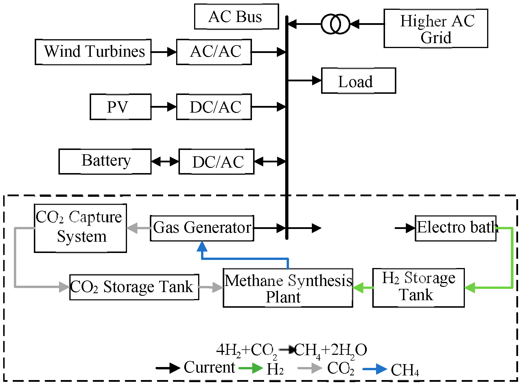
The studied MEMG architecture, as shown in Figure 1, integrates multiple generation, conversion, and storage technologies. The energy sources consist of wind turbines (WTs), photovoltaic (PV) systems, and a gas turbine (GT). For energy conversion, the system incorporates an electrolyzer (EL) to produce hydrogen and a methanation unit to synthesize natural gas (CH₄). Energy storage is provided by batteries (EES), a hydrogen storage tank (H₂), and a carbon dioxide storage tank (CO₂). The model operates under the assumption that network losses are negligible.

2.1. Objective Function

To address the impact of uncertainty on capacity planning, the objective of this model is to minimize the total annual comprehensive cost, denoted as $C_{total}$. This cost function is formulated as a weighted sum of economic and low-carbon objectives:

$$\min C_{total}={\omega }_1{C}_{econ}+{\omega }_2{C}_{carbon}$$

(1)

where ${\omega }_1$ and ${\omega }_2$ are the weighting factors for the economic and low-carbon objectives, respectively. In this study, equal weighting is adopted, with both set to 1/2. The economic cost $C_{econ}$ encompasses the entire lifecycle cost of the microgrid, comprising three components:

$$C_{econ}=C_{invest}+C_{om}+C_{oper}$$

(2)

Here,

• $C_{invest}$: Annualized investment cost.
• $C_{om}$: Annual operation and maintenance (O&M) cost.
• $C_{oper}$: Annual operating cost (encompassing energy and carbon-related expenses).

The calculation for each cost component is detailed below.

2.1.1. Annual Equipment Investment Cost ($C_{invest}$)

This cost component represents the annualized capital expenditure for all installed equipment, calculated as

$$C_{invest}=\sum _i^{Devices}{c}_i^{inv} P_i^{rated}{CRF}_i$$

(3)

In the formula, $c_i^{inv}$ represents the unit investment cost of different equipment units; WT, PV, GT, CCS, EL, CH₄, and EES stand for wind turbines, photovoltaic systems, gas generators, carbon capture facilities, electrolyzers, methanation equipment, and batteries, respectively; $P_i^{rated}$ denotes the rated installed capacity of the equipment; $CR{F}_i$ is the capital recovery coefficient for device $i$.

The $CR{F}_i$ calculation is shown in (4):

$${CRF}_i={\displaystyle \frac{{r(1+r)}^{n_i}}{{(1+r)}^{n_i}-1}}$$

(4)

where $r$ is the discount rate, and $n_i$ is the operational lifetime of device $i$.

2.1.2. Annual Operating Cost and Maintenance Cost (C_om)

This cost accounts for fixed annual maintenance expenses, assumed proportional to the installed capacity:

$$C_{om}=\sum _i^{Devices}(k_{1,i}+k_{2,i})c_i^{inv} P_i^{rated}$$

(5)

Here, $k_{1,i}$ and $k_{2,i}$ are the O&M cost coefficients, expressed as ratios to the investment cost for device $i$.

2.1.3. Annual Operating Cost ($C_{oper}$)

This component aggregates variable costs incurred during daily operations over representative days. It includes expenses related to energy transactions, demand response compensation, and environmental compliance:

$$C_{oper}=C_{gird}+C_{DR}+C_{gas}+C_{curt}+C_{TCT}$$

(6)

where

• $C_{grid}$: Cost of electricity purchased from the main grid.
• $C_{DR}$: Demand response compensation cost.
• $C_{gas}$: Cost of natural gas procurement.
• $C_{curt}$: Penalty cost for wind and photovoltaic power curtailment.
• $C_{TCT}$: Tiered carbon trading cost.

The calculation methodology for each term in $C_{oper}$ is provided in the subsequent subsections.

Cost of Electricity Purchased by the Superiors

The cost of electricity imported from the main grid is given by

$$\begin{array}{c}{F}_{\mathrm{grid}}=\end{array}{\displaystyle \sum _{d\in {\mathbf{\Omega }}_{\mathrm{D}}}{\displaystyle \sum _t^{24}{N}_{\mathrm{d}\mathrm{a}\mathrm{y}}\left(c_{\mathrm{grid},d,t}{P}_{\mathrm{grid},d,t}\right) }}$$

(7)

In the formula, ${\mathbf{\Omega }}_{\mathrm{D}}$ is the set of four typical days, including spring, summer, autumn, and winter; $N_{\mathrm{d}\mathrm{a}\mathrm{y}}$ refers to the number of days that a typical day d occupies in a year; and $c_{\mathrm{grid},d,t}$ is the time price of a typical day d.

Demand Response Compensation Cost

The compensation cost for demand response participants is calculated as

$$\begin{array}{c}{F}_{\mathrm{D}\mathrm{R}}=\end{array}{\displaystyle \sum _{d\in {\Omega }_D}{\displaystyle \sum _t^{24}{N}_{\mathrm{d}\mathrm{a}\mathrm{y}}\left({\delta }_{\mathrm{z}}\left|\Delta P_{\mathrm{e},\mathrm{Load},d,t}^z\right|\right) }}$$

(8)

In the formula, ${\delta }_{\mathrm{z}}$ represents the unit compensation coefficient of the transferable load participating in DR.

Gas Cost

Gas cost is shown in (9):

$$\begin{array}{c}{F}_{\mathrm{fuel}}={\displaystyle \sum _{d\in {\Omega }_{\mathrm{D}}}{\displaystyle \sum _t^{24}{N}_{\mathrm{d}\mathrm{a}\mathrm{y}}\left(c_{{\mathrm{CH}}_4,d,t}\left({\tau }_{\mathrm{GT}}{P}_{\mathrm{G}\mathrm{T},r}- V_{\mathrm{C}{\mathrm{O}}_2,d,t}^{\mathrm{P}2\mathrm{G}}\right)\right) }}\end{array}$$

(9)

In the formula, $c_{{\mathrm{CH}}_4,d,t}$ is the unit price of natural $\left({\tau }_{\mathrm{GT}}{P}_{\mathrm{G}\mathrm{T},\mathrm{r}}- V_{\mathrm{C}{\mathrm{O}}_2,d,t}^{\mathrm{P}2\mathrm{G}}\right)$ gas purchased in the t period of a typical day d.

Cost of Wind and Light Abandonment

Cost of wind and light abandonment is shown in (10):

$$F_{\mathrm{c}\mathrm{u}\mathrm{t}}=\begin{array}{c}{\displaystyle \sum _{d\in {\Omega }_{\mathrm{D}}}{\displaystyle \sum _t^{24}{N}_{\mathrm{d}\mathrm{a}\mathrm{y}}\left({\chi }_{\mathrm{wt}}{P}_{\mathrm{W}\mathrm{T},d,t}^{\mathrm{c}\mathrm{u}\mathrm{t}}+{\chi }_{\mathrm{p}\mathrm{v}}{P}_{\mathrm{P}\mathrm{V},d,t}^{\mathrm{c}\mathrm{u}\mathrm{t}}\right) }}\end{array}$$

(10)

In the formula, $P_{\mathrm{W}\mathrm{T},d,t}^{\mathrm{c}\mathrm{u}\mathrm{t}}$ and $P_{\mathrm{P}\mathrm{V},d,t}^{\mathrm{c}\mathrm{u}\mathrm{t}}$ are the wind curtailment power and ${\chi }_{\mathrm{wt}}$ light ${\chi }_{\mathrm{wt}}$ curtailment power in the t time period of a typical day d and they represent the penalty cost per unit of wind curtailment power and light curtailment power.

Carbon Trading Costs

Carbon trading costs are shown in (11):

$$F_{\mathrm{C}{\mathrm{O}}_2}={\displaystyle \sum _{d\in {\Omega }_{\mathrm{D}}}{\displaystyle \sum _t^{24}{N}_{\mathrm{d}\mathrm{a}\mathrm{y}}{f}_{\mathrm{C}{\mathrm{O}}_2,d,t} }}$$

(11)

In the formula, $f_{\mathrm{C}{\mathrm{O}}_2,d,t}$ is the step carbon trading cost at time t of a typical day d.

2.2. Model Constraints

2.2.1. Constraints

The installed capacity of each device is bounded by its upper and lower limits:

$$P_i^{\mathrm{m}\mathrm{i}\mathrm{n}}\le P_i^{rated}\le P_i^{\mathrm{m}\mathrm{a}\mathrm{x}},\forall i\in \mathcal{D}$$

(12)

where the superscripts min and max denote the minimum and maximum allowable installed capacities, respectively.

2.2.2. Power Balance Constraints

The electrical power balance within the microgrid must be maintained at all times:

$$\begin{array}{l}{P}_{\mathrm{grid},d,t}+P_{\mathrm{PV},d,t}+P_{\mathrm{WT},d,t}+{\mathrm{P}}_{\mathrm{ESS},d,t}^{\mathrm{dis}}+P_{\mathrm{GT},d,t}=\\ P_{\mathrm{CCS},d,t}+P_{\mathrm{EL},d,t}+{\mathrm{P}}_{\mathrm{ESS},d,t}^{\mathrm{ch}}+P_{{\mathrm{CH}}_4,d,t}+P_{\mathrm{e},\mathrm{Load},d,t}\end{array}$$

(13)

In the formula, $P_{\mathrm{e},\mathrm{Load},d,t}$ is the power load of users in the t period of a typical day d.

2.2.3. Wind Power Output Constraints

Wind power output constraint is shown in (14) and (15):

$$\begin{array}{c}0\le P_{\mathrm{W}\mathrm{T},d,t}\le P_{\mathrm{W}\mathrm{T},\mathrm{r}}\end{array}$$

(14)

$$\begin{array}{c}0\le P_{\mathrm{P}\mathrm{V},d,t}\le P_{\mathrm{P}\mathrm{V},\mathrm{r}}\end{array}$$

(15)

In the formula, $P_{\mathrm{W}\mathrm{T},d,t}$ and $P_{\mathrm{P}\mathrm{V},d,t}$ are the power of a typical day d and wind and light equipment t.

2.2.4. Gas-Generating Constraints

In addition, gas-generating units and carbon capture equipment need to meet the following constraints, which are shown in (16)–(19):

$$\begin{array}{c}0\le P_{\mathrm{G}\mathrm{T},d,t}\le P_{\mathrm{GT},\mathrm{r}}\end{array}$$

(16)

$$\begin{array}{c}{P}_{\mathrm{G}\mathrm{T},d,t}-P_{\mathrm{G}\mathrm{T},d,t-1}\le \Delta P_{\mathrm{G}\mathrm{T}}^{\mathrm{RU},\max }\end{array}$$

(17)

$$\begin{array}{c}{P}_{\mathrm{G}\mathrm{T},d,t-1}-P_{\mathrm{G}\mathrm{T},d,t}\le \Delta P_{\mathrm{G}\mathrm{T}}^{\mathrm{RD},\max }\end{array}$$

(18)

$$F(P_{\mathrm{G}\mathrm{T},t})=a{P}_{\mathrm{G}\mathrm{T},t}+b{P}_{\mathrm{G}\mathrm{T},\mathrm{r}}$$

(19)

In the formula, $F(P_{\mathrm{G}\mathrm{T},t})$ is the gas consumption of $P_{\mathrm{G}\mathrm{T},t}$, the gas generator in the t period; the output $P_{\mathrm{G}\mathrm{T},\mathrm{r}}$ is the power of the gas generator in the t period and is the rated total power of the gas generator; a and b are the slope and intercept of the gas cost curve, respectively; $P_{\mathrm{G}\mathrm{T},d,t}$ is the power of the gas generator set in $\Delta P_{\mathrm{G}\mathrm{T}}^{\mathrm{RU},\max }$ and $\Delta P_{\mathrm{G}\mathrm{T}}^{\mathrm{RD},\max }$, the t period of the typical day d, and are the maximum climbing and descending capacity limits of the gas generator.

2.2.5. Carbon Capture Equipment Constraints

Carbon capture equipment is shown in (20)–(24).

The carbon capture system operates coupled with the gas turbine. Gas turbines generate carbon dioxide emissions ${\mathrm{E}}_{{\mathrm{C}\mathrm{O}}_2,\mathrm{e}\mathrm{m}\mathrm{i}\mathrm{t}\left(\mathrm{t}\right)}$ during operation. The CCS equipment captures a portion of these emissions, where the captured amount ${\mathrm{E}}_{{\mathrm{C}\mathrm{O}}_2,\mathrm{e}\mathrm{m}\mathrm{i}\mathrm{t}\left(\mathrm{t}\right)}$ depends on its operating power ${\mathrm{P}}_{\mathrm{C}\mathrm{C}\mathrm{S}\left(\mathrm{t}\right)}$. The captured CO₂ is compressed and stored in a carbon storage tank, ready to be utilized by the P2G process or sequestered. Equations (20)–(24) describe the mathematical model of this process, including capture efficiency, equipment operating power, and its ramping constraints.

In this paper, the amount of CO₂ captured by CCS varies with the load and the output of the gas generator. Therefore, the amount of carbon capture in CCS involves the output of the gas generator, which is usually modeled:

$$\begin{array}{c}{V}_{{\mathrm{CO}}_2,d,t}^{\mathrm{GT}}=e_{\mathrm{GT}}{P}_{\mathrm{GT},d,t}\end{array}$$

(20)

In the formula, $V_{{\mathrm{CO}}_2,d,t}^{\mathrm{GT}}$ is the carbon emission of the gas generator, and $P_{\mathrm{GT},d,t}$ and $e_{\mathrm{GT}}$ are the output of the gas generator and the carbon emission coefficient related to its output.

Because of the loss of equipment, efficiency cannot reach 100%. The relationship between the amount of CO₂ captured and the total amount of discharge is given by the formula shown in (21):

$$\begin{array}{c}{V}_{{\mathrm{CO}}_2,d,t}^{\mathrm{CCS}}={\eta }^{\mathrm{CCS}}{V}_{{\mathrm{CO}}_2,d,t}^{\mathrm{GT}}\end{array}$$

(21)

In addition, gas-generating units and carbon capture equipment need to meet the following constraints as shown in (22)–(24):

$$\begin{array}{c}0\le P_{\mathrm{C}\mathrm{C}\mathrm{S},d,t}^{\mathrm{C}{\mathrm{O}}_2}\le P_{\mathrm{C}\mathrm{C}\mathrm{S},\mathrm{r}}\end{array}$$

(22)

$$\begin{array}{c}{P}_{\mathrm{C}\mathrm{C}\mathrm{S},d,t}-P_{\mathrm{C}\mathrm{C}\mathrm{S},d,t-1}\le \Delta P_{\mathrm{C}\mathrm{C}\mathrm{S}}^{\mathrm{RU},\max }\end{array}$$

(23)

$$\begin{array}{c}{P}_{\mathrm{C}\mathrm{C}\mathrm{S},d,t-1}-P_{\mathrm{C}\mathrm{C}\mathrm{S},d,t}\le \Delta P_{\mathrm{C}\mathrm{C}\mathrm{S}}^{\mathrm{RD},\max }\end{array}$$

(24)

In the formula, $P_{\mathrm{C}\mathrm{C}\mathrm{S},d,t}^{\mathrm{C}{\mathrm{O}}_2}$ is the ideal power consumption of the carbon; $P_{\mathrm{C}\mathrm{C}\mathrm{S},d,t}$ is the power consumption of the carbon capture equipment in the t period of a typical day d CCS; and $\Delta P_{\mathrm{C}\mathrm{C}\mathrm{S}}^{\mathrm{RU},\max }$ and $\Delta P_{\mathrm{C}\mathrm{C}\mathrm{S}}^{\mathrm{RD},\max }$ are the maximum climbing and descending capacity limits of the carbon capture equipment.

This research focuses on the steady-state operation economics and carbon benefits of the CCS-P2G system but does not consider its dynamic start-up/shutdown costs. This simplification is common in preliminary research and strategic-level configuration analysis, helping to reduce model complexity.

2.2.6. Electrolytic Cell Constraints

The power and climbing power of the electrolytic cell are limited by the equipment, and the following inequality constraints are shown in (25)–(27):

$$0\begin{array}{c}\le P_{\mathrm{E}\mathrm{L},d,t}\le P_{\mathrm{E}\mathrm{L},\mathrm{r}}\end{array}$$

(25)

$$\begin{array}{c}{P}_{\mathrm{E}\mathrm{L},d,t}-P_{\mathrm{E}\mathrm{L},d,t-1}\le \Delta P_{\mathrm{E}\mathrm{L}}^{\mathrm{RU},\max }\end{array}$$

(26)

$$\begin{array}{c}{P}_{\mathrm{E}\mathrm{L},d,t-1}-P_{\mathrm{E}\mathrm{L},d,t}\le \Delta P_{\mathrm{E}\mathrm{L}}^{\mathrm{RD},\max }\end{array}$$

(27)

In the formula, $P_{\mathrm{E}\mathrm{L},d,t}$ is the power of the electrolytic cell equipment in the t period of a typical day, and $\Delta P_{\mathrm{E}\mathrm{L}}^{\mathrm{RU},\max }$ and $\Delta P_{\mathrm{E}\mathrm{L}}^{\mathrm{RD},\max }$ are the maximum limits of the climbing and descending capacities of the electrolytic cell.

2.2.7. Methanation Equipment Constraints

Power-to-gas technology converts surplus electrical energy into easily storable natural gas, serving as a key solution for cross-seasonal energy storage and carbon recycling. The P2G process modeled in this paper consists of two consecutive stages:

The electrolyzer consumes electrical power PEL(t) to split water, producing hydrogen H₂ and oxygen.

The methanation unit utilizes the hydrogen produced in the previous step and the carbon dioxide ${CO}_2$ captured by the CCS to perform a catalytic reaction, synthesizing methane ${CH}_4$.

The produced methane can be directly fed into the gas turbine for power generation or injected into the natural gas grid. Equations (28)–(33) describe the energy and mass balance relationships of the aforementioned two stages and the operational constraints of the equipment.

The electrical power generated by the methanation equipment in P2G devices is related to the unit power consumption coefficient. The total power of P2G devices can be divided into two main parts: the first stage involves electrolyzing water in the electrolyzer to produce hydrogen and oxygen. In the second stage, CO₂ reacts with H₂ under the action of a catalyst to synthesize CH₄ and water. Therefore, the following formula can be used for calculation as shown in (28)–(33):

$$\begin{array}{c}{P}_{P2G,t}=P_{\mathrm{EL},t}+P_{\mathrm{C}{\mathrm{H}}_4,t}\end{array}$$

(28)

$$\begin{array}{c}{V}_{{\mathrm{CH}}_4,t}={\omega }_1{V}_{{\mathrm{CO}}_2,t}^{\mathrm{P}2\mathrm{G}}\end{array}$$

(29)

$$\begin{array}{c}{P}_{\mathrm{C}{\mathrm{H}}_4,d,t}={\lambda }_{\mathrm{C}{\mathrm{H}}_4}{V}_{\mathrm{C}{\mathrm{H}}_4,d,t}\end{array}$$

(30)

$$\begin{array}{c}0\le P_{\mathrm{C}{\mathrm{H}}_4,d,t}\le P_{\mathrm{C}{\mathrm{H}}_4,\mathrm{r}}\end{array}$$

(31)

$$\begin{array}{c}{P}_{\mathrm{C}{\mathrm{H}}_4,d,t-1}-P_{\mathrm{C}{\mathrm{H}}_4,d,t}\le \Delta P_{\mathrm{C}{\mathrm{H}}_4}^{\mathrm{RD},\max }\end{array}$$

(32)

$$\begin{array}{c}{P}_{\mathrm{C}{\mathrm{H}}_4,d,t}-P_{\mathrm{C}{\mathrm{H}}_4,d,t-1}\le \Delta P_{\mathrm{C}{\mathrm{H}}_4}^{\mathrm{RU},\max }\end{array}$$

(33)

In the formula, $P_{\mathrm{P}2\mathrm{G},t}$ is the power consumption of P2G equipment; ${\omega }_1$ is the gas reaction equilibrium coefficient; $V_{{\mathrm{CO}}_2,t}^{\mathrm{P}2\mathrm{G}}$ is the amount of CO₂ required for synthesis of CH₄; $P_{\mathrm{C}{\mathrm{H}}_4,d,t}$ is the power of the t period in a typical day for electrolytic cell equipment; ${\lambda }_{{\mathrm{CH}}_4}$ is the power consumption coefficient of the CH₄ unit; and $\Delta P_{\mathrm{E}\mathrm{L}}^{\mathrm{RD},\max }$ and $\Delta P_{{\mathrm{C}\mathrm{H}}_4}^{\mathrm{RU},\max }$ are the maximum limits of climbing and descending capacities of the electrolytic cell.

2.2.8. Generic Energy Storage Constraints

Hydrogen storage (H₂) and carbon storage (CO₂) systems share similar operational characteristics. Therefore, this paper employs a unified generic energy storage model to describe their operational constraints, as defined by the following equations.

State-of-Charge (SoC) Update Constraint:

$$S_{d,t}=S_{d,t-1}+{\eta }_{ch}\cdot P_{ch,d,t}\cdot \Delta t-{\displaystyle \frac{P_{disch,d,t}}{{\eta }_{disch}}}\cdot \Delta t$$

(34)

This equation governs the energy state evolution of the storage device. Here, $S_{d,t}$ represents the storage level at time $t$ of typical day $d$, corresponding to $E_{H_2}(d,t)$ for H₂ storage and $E_{{CO}_2}(d,t)$ for CO₂ storage. ${\eta }_{ch}$ and ${\eta }_{disch}$ are the charging and discharging efficiencies, respectively. $P_{ch,d,t}$ and $P_{disch,d,t}$ denote the charging and discharging powers during the time interval $\Delta t$.

Power Boundary Constraints:

$$0\le P_{ch,d,t}\le u_{d,t}\cdot P_{ch}^{\mathrm{m}\mathrm{a}\mathrm{x}}$$

(35)

$$0\le P_{disch,d,t}\le \left(1-u_{d,t}\right)\cdot P_{disch}^{\mathrm{m}\mathrm{a}\mathrm{x}}$$

(36)

These inequalities ensure that the charging and discharging powers do not exceed the device’s maximum ratings. The binary variable $u_{d,t}$ prevents simultaneous charging and discharging.

State-of-Charge Boundary Constraint:

$$S^{\mathrm{m}\mathrm{i}\mathrm{n}}\le S_{d,t}\le S^{\mathrm{m}\mathrm{a}\mathrm{x}}$$

(37)

This constraint maintains the energy state of the storage device within its permissible minimum and maximum limits for safe and stable operation.

For clarity, the correspondence between the parameters of the hydrogen/carbon storage devices and the generic model variables is summarized in

Table 1. Mapping between generic storage model and specific device parameters.

Generic Model Var/Param	H2 Storage Correspondence and Meaning	CO2 Storage Correspondence and Meaning
$S_{d,t}$	$E_{H_2}(d,t)$: H2 storage level at t (m3)	$E_{{CO}_2}(d,t)$: CO2 storage level at t (m3)
$P_{ch,d,t}$	$P_{H_2,in}(d,t)$: H2 charging power (kW)	$P_{{CO}_2,in}(d,t)$: CO2 charging power (kW)
$P_{disch,d,t}$	$P_{H_2,out}(d,t)$: H2 discharging power (kW)	$P_{{CO}_2,out}(d,t)$: CO2 discharging power (kW)
${\eta }_{ch}$	${\eta }_{H_2,ch}$: H2 charging efficiency	${\eta }_{{CO}_2,ch}$: CO2 charging efficiency
${\eta }_{disch}$	${\eta }_{H_2,disch}$: H2 discharging efficiency	${\eta }_{{CO}_2,disch}$: CO2 discharging efficiency
$P_{ch}^{\mathrm{m}\mathrm{a}\mathrm{x}}$	$P_{H_2,in}^{\mathrm{m}\mathrm{a}\mathrm{x}}$: Max H2 charging power (kW)	$P_{{CO}_2,in}^{\mathrm{m}\mathrm{a}\mathrm{x}}$: Max CO2 charging power (kW)
$P_{disch}^{\mathrm{m}\mathrm{a}\mathrm{x}}$	$P_{H_2,out}^{\mathrm{m}\mathrm{a}\mathrm{x}}$: Max H2 discharging power (kW)	$P_{{CO}_2,out}^{\mathrm{m}\mathrm{a}\mathrm{x}}$: Max CO2 discharging power (kW)
$S^{\mathrm{m}\mathrm{i}\mathrm{n}}$	$E_{H_2}^{\mathrm{m}\mathrm{i}\mathrm{n}}$: Min H2 storage capacity (m3)	$E_{{CO}_2}^{\mathrm{m}\mathrm{i}\mathrm{n}}$: Min CO2 storage capacity (m3)
$S^{\mathrm{m}\mathrm{a}\mathrm{x}}$	$E_{H_2}^{\mathrm{m}\mathrm{a}\mathrm{x}}$: Max H2 storage capacity (m3)	$E_{{CO}_2}^{\mathrm{m}\mathrm{a}\mathrm{x}}$: Max CO2 storage capacity (m3)

.

A core innovation of the microgrid model proposed in this paper is the synergistic coupling of CCS and P2G technologies. This integration establishes an internal ‘carbon cycle’: CO₂ emitted by the gas turbine is captured by the CCS, and the captured CO₂ is subsequently utilized as a feedstock in the P2G process. There, it combines with H₂—produced via water electrolysis powered by renewable energy—to synthesize carbon-neutral methane (CH₄). This pathway not only reduces the system’s net carbon emissions but also enhances the accommodation capacity of renewable energy, achieving synergistic optimization of energy and environmental objectives.

2.2.9. Battery Constraints

The constraints for the battery energy storage system (BESS) are consistent with the generic energy storage model and are described by the following equations:

$$\begin{array}{c}{P}_{EES,t}=P_{ESS,t-1}+\left(P_{\mathrm{ESS},t}^{ch}{\eta }_{\mathrm{ch}}-{\displaystyle \frac{P_{ESS,t}^{dis}}{{\eta }_{\mathrm{dis}}}}\right)\end{array}$$

(38)

$$\begin{array}{c}0\le P_{\mathrm{ESS},\mathrm{d},t}^{\mathrm{ch}}\le Y_{\mathrm{ESS},\mathrm{d},t}{P}_{\mathrm{ch}}^{\max }\end{array}$$

(39)

$$\begin{array}{c}0\le P_{\mathrm{ESS},\mathrm{d},t}^{\mathrm{dis}}\le \left(1-Y_{\mathrm{ESS},\mathrm{d},t}\right)P_{\mathrm{dis}}^{\max }\end{array}$$

(40)

$$\begin{array}{c}{P}_{\mathrm{EES},1}=P_{\mathrm{EES},\mathrm{T}}\end{array}$$

(41)

In the formula, ${\eta }_{\mathrm{ch}}$ and ${\eta }_{\mathrm{dis}}$ are the charging and discharging coefficients of the battery; $P_{\mathrm{ESS},t}^{\mathrm{c}\mathrm{h}}$ and $P_{\mathrm{E}\mathrm{S}\mathrm{S},t}^{\mathrm{d}\mathrm{i}\mathrm{s}}$ are the charging and discharging powers of the battery in the t period; $P_{\mathrm{E}\mathrm{S}\mathrm{S},d,t}^{\mathrm{c}\mathrm{h}}$ and $P_{\mathrm{E}\mathrm{S}\mathrm{S},d,t}^{\mathrm{d}\mathrm{i}\mathrm{s}}$ are the charging and discharging powers of the battery in the t period of the typical day d; $Y_{\mathrm{E}\mathrm{S}\mathrm{S},t}$ is the binary variable of the charging and discharging state of the battery in the t period of the typical day d; $P_{\mathrm{ch}}^{\max }$ and $P_{\mathrm{dis}}^{\max }$ are the maximum charging and discharging powers of the battery; T is the scheduling cycle.

2.2.10. Power Purchase Constraints

Power purchase constraint is shown in (42).

Because the output of distributed energy has strong randomness and volatility, this paper only considers purchasing electricity from the superior power grid.

$$0\le P_{\mathrm{grid},d,t}\le P_{\mathrm{grid}}^{\max }$$

(42)

In the formula, $P_{\mathrm{grid}}^{\max }$ is the maximum value of power purchase $P_{\mathrm{grid}}^{\max }$ from the superior in the t period of a typical day d and does not exceed the maximum output of wind and solar equipment.

2.2.11. Wind and Light Power Constraints

Wind and light power constraints are shown in (43) and (44):

$$0\le {\displaystyle \frac{{\displaystyle \sum _t}{P}_{\mathrm{PV},d,t}^{\mathrm{cut}}}{{\displaystyle \sum _t}{P}_{\mathrm{PV},d,t}}}\le {\gamma }_{\mathrm{pv}}^{\mathrm{cut}}$$

(43)

In the formula, ${\gamma }_{\mathrm{pv}}^{\mathrm{cut}}$ is the maximum light loss rate.

$$0\le {\displaystyle \frac{{\displaystyle \sum _t}{P}_{\mathrm{WT},d,t}^{\mathrm{cut}}}{{\displaystyle \sum _t}{P}_{\mathrm{WT},d,t}}}\le {\gamma }_{\mathrm{wt}}^{\mathrm{cut}}$$

(44)

In the formula, ${\gamma }_{\mathrm{wt}}^{\mathrm{cut}}$ is the maximum wind curtailment rate.

2.2.12. H₂ Balance Constraints

The H₂ balance constraints are shown in (45):

$$\begin{array}{c}{V}_{{\mathrm{H}}_2,d,t}^{\mathrm{EL}}+V_{{\mathrm{H}}_2,d,t}^{\mathrm{s}\mathrm{t}\text{-}\mathrm{out}}=V_{{\mathrm{H}}_2,d,t}^{\mathrm{P}2\mathrm{G}}+V_{{\mathrm{H}}_2,d,t}^{\mathrm{s}\mathrm{t}\text{-}\mathrm{i}\mathrm{n}}\end{array}$$

(45)

2.2.13. CO₂ Balance Constraints

The CO₂ Balance constraints are shown in (46):

$$V_{{\mathrm{CO}}_2,d,t}^{\mathrm{ccs}}+V_{{\mathrm{CO}}_2,d,t}^{\mathrm{st}\text{-}\mathrm{out}}=V_{{\mathrm{CO}}_2,d,t}^{\mathrm{P}2\mathrm{G}}+V_{{\mathrm{CO}}_2,d,t}^{\mathrm{st}\text{-}\mathrm{in}}$$

(46)

2.2.14. Ladder-Type Carbon Trading Constraints

By trading carbon emission allowances, the government or relevant departments allocate certain carbon emission quotas to power generation companies that have emissions, either for a fee or free of charge, to achieve carbon reduction targets. Production is positively correlated with carbon quotas; for companies of the same capacity, those with stronger emission reduction capabilities generate surplus quotas, while others face deficits, as can be found in [24,25]. Moreover, the gradual tightening of national $D_{\mathrm{c}}$ carbon quotas has increased the trading price of carbon quotas. To boost profits, companies are forced to reduce their carbon emissions. If they exceed their allocated quotas, they must purchase the shortfall from other companies or institutions. Free carbon emission allowances can be expressed as follows:

$$\begin{array}{c}{D}_{\mathrm{c}}={\alpha }_{\mathrm{gt}}{\displaystyle \sum _t}{P}_{\mathrm{GT},t}+{\alpha }_{\mathrm{tp}}{\displaystyle \sum _t}{P}_{\mathrm{grid},t}\end{array}$$

(47)

$D_{\mathrm{c}}$ is the carbon quota for the system; ${\alpha }_{\mathrm{gt}}$ is the emission quota for the unit power generation of gas generators purchased by the superior; ${\alpha }_{\mathrm{tp}}$ is the generation of thermal power purchased by the superior; $P_{\mathrm{GT},t}$ is the output power of gas generators in the t period; $P_{\mathrm{grid},t}$ is the power purchased by the superior grid.

The actual carbon emissions in the $E_{\mathrm{c}}$ microgrid are shown in (48):

$$\begin{array}{c}{E}_{\mathrm{c}}={\beta }_{\mathrm{gt}}{\displaystyle \sum _t}{P}_{\mathrm{GT},t}+{\beta }_{\mathrm{tp}}{\displaystyle \sum _t}{P}_{\mathrm{grid},t}-V_{{\mathrm{CO}}_2,t}^{\mathrm{ccs}}/\end{array}{\rho }_{{\mathrm{CO}}_2}$$

(48)

$E_{\mathrm{c}}$ is the cruel carbon emission; ${\beta }_{\mathrm{gt}}$ is the carbon emission intensity per unit of electricity ${\beta }_{\mathrm{gt}}$ generated by gas generators; carbon emission ${\rho }_{{\mathrm{CO}}_2}$ is the CO₂ density intensity per unit of electricity generated by thermal power purchased by superiors; the above data are referenced in the literature [11].

To further increase carbon emission costs and incentivize emission reduction, a tiered carbon trading model is adopted in this paper. This model imposes an increasing carbon price based on the interval in which the difference between the actual carbon emissions and the free quota, $\Delta E=E_{actual}-E_{free}$, falls. The calculation mechanism is described step-by-step as follows:

Define Intervals and Prices:

Let the base carbon price be $p$ (CNY/ton), the price growth rate be $\alpha$, and the length of a single interval be $L$ (tons). The carbon emission range is divided into multiple tiers. The $k$-th tier ($k=\mathrm{1,2},3,\dots$) is defined as $\left[\right(k-1)L, kL)$, and its corresponding carbon price $p_k$ increases geometrically: $p_k=p\cdot (1+\alpha {)}^{k-1}$.

Calculate Tiered Cost:

The total tiered carbon trading cost $C_{TCT}$ is the sum of the costs across all applicable tiers. For a given emission difference $\Delta E$, assuming it falls within the $m$-th tier (i.e., $(m-1)L<\Delta E\le mL$), the cost is calculated as

$$C_{TCT}=p\cdot L\cdot \sum _{k=1}^{m-1}(1+\alpha {)}^{k-1}+p\cdot (1+\alpha {)}^{m-1}\cdot [\Delta E-(m-1\left)L\right]$$

(49)

The first term in this formula computes the cumulative cost of the first $m-1$ fully loaded intervals, and the second term computes the cost for the partially filled $m$-th interval.

For easier implementation within the optimization model, this piecewise linear cost function can be equivalently formulated using the following compact mathematical programming form, which captures the structure more clearly than the original Equation (50):

$$C_{TCT}=\sum _{k=1}^K{p}_k\cdot \Delta E_k$$

(50)

Subject:

$$\Delta E=\sum _{k=1}^K\Delta E_k$$

(51)

$$0\le \Delta E_k\le L,\forall k\in \left\{\mathrm{1,2},\dots ,K-1\right\}$$

(52)

$$0\le \Delta E_K$$

(53)

where $K$ is a sufficiently large constant, representing the maximum number of tiers considered. $\Delta E_k$ is an auxiliary decision variable, representing the portion of the emission difference $\Delta E$ that falls into the $k$-th price tier. $p_k=p\cdot (1+\alpha {)}^{k-1}$ is the carbon price for the $k$-th tier.

2.2.15. Incentive Demand Response Constraints

The incentive-based demand response (DR) model adopted in this paper simplifies the adjustment of power consumption strategies. It focuses on the load acquisition facilitated by national policy subsidies during load shifting, without considering changes in consumption patterns due to electricity price adjustments, aiming to improve the microgrid’s economy. Furthermore, loads are categorized in a simplified manner [26,27].

The total electrical load is divided into two parts: inelastic load and shiftable load. The shiftable load can be transferred across time dimensions and possesses DR capability. This is expressed as

$$\begin{array}{c}{P}_{\mathrm{e},\mathrm{Load},t}=P_{\mathrm{e},\mathrm{Load},t}^{\mathrm{q},0}+P_{\mathrm{e},\mathrm{Load},t}^{\mathrm{z},0} \end{array}$$

(54)

In the formula, $P_{\mathrm{e},\mathrm{Load},t}$ represents the value $P_{\mathrm{e},\mathrm{Load},t}^{\mathrm{q},0}$ of the load t period, represents the forced $P_{\mathrm{e},\mathrm{Load},t}^{\mathrm{z},0}$ load of the electric load t period, and represents the transferable load of the load t period.

The inelastic load $P_{fixed,d,t}$ must be consumed and typically refers to essential energy uses in daily life, such as lighting and refrigeration. This fixed load is not considered to participate in DR.

The shiftable load $P_{shift,d,t}$ can be transferred to different time periods during operation if necessary. Generally, consumption is reduced during peak load periods and increased during low load periods to improve resource utilization. The constraints are as follows:

$$\begin{array}{c}{P}_{\mathrm{e},\mathrm{Load},t}^{\mathrm{z}}=P_{\mathrm{e},\mathrm{Load},t}^{\mathrm{z},0}+\Delta P_{\mathrm{e},\mathrm{Load},t}^{\mathrm{z}} \end{array}$$

(55)

$$\begin{array}{c}\Delta P_{\mathrm{e},\mathrm{Load},t}^{\mathrm{z}}={\zeta }_{\mathrm{e},t}^{\mathrm{t}}{P}_{\mathrm{e},\mathrm{Load},t}^{\mathrm{z}\text{-}\mathrm{in}}-\left(1-{\zeta }_{\mathrm{e},t}^{\mathrm{z}}\right)P_{\mathrm{e},\mathrm{Load},t}^{\mathrm{z}\text{-}\mathrm{out}}\end{array}$$

(56)

$$\begin{array}{c} \end{array}{\displaystyle \sum }_t\Delta P_{\mathrm{e},\mathrm{Load},t}^z=0$$

(57)

$$\begin{array}{c}{\mathit{\tau }}_{\mathrm{e},t}^{\min }\le \Delta P_{\mathrm{e},\mathrm{Load},t}^{\mathrm{z}}\le \end{array}{\mathit{\tau }}_{\mathrm{e},t}^{\max }$$

(58)

In the formula, $P_{\mathrm{e},\mathrm{Load},t}^{\mathrm{z}}$ and $\Delta P_{\mathrm{e},\mathrm{Load},t}^{\mathrm{z}}$ represent the amount of transferable ${\zeta }_{\mathrm{e},t}^{\mathrm{z}}$ load DR and the amount participating in DR; $P_{\mathrm{e},\mathrm{Load},t}^{\mathrm{z}\text{-}\mathrm{in}}$ is $P_{\mathrm{e},\mathrm{Load},t}^{\mathrm{z}\text{-}\mathrm{out}}$, a binary variable indicating the access status of DR at time t, and represents the incoming and outgoing power of transferable ${\mathit{\tau }}_{\mathrm{e},t}^{\min }$ load ${\mathit{\tau }}_{\mathrm{e},t}^{\max }$; $\Delta P_{\mathrm{e},\mathrm{Load},t}^{\mathrm{z}}$ in Equation (57) indicates that the total power change of the transferable load participating in DR within a scheduling cycle does not affect the original load and represents the upper and lower limit values of the amount participating in DR at each time period.

Incentive Demand Response Mechanism

To enhance the economic performance of the microgrid, this paper adopts a shiftable load management strategy within the framework of incentive-based demand response. This mechanism does not rely on electricity price variations. Instead, the microgrid operator enters into agreements with users and provides fixed compensation to participants for shifting part of their electricity consumption from peak periods to off-peak periods.

The electrical load is simplified into two parts: rigid load and shiftable load. The rigid load must be satisfied instantly, while the shiftable load (e.g., electric vehicle charging, specific industrial processes) can be shifted across time dimensions. It is assumed that the shiftable load constitutes a proportion ${\alpha }_{shift}$ of the total load, and its total energy consumption remains unchanged within the dispatch cycle.

Demand Response Parameter Setting

In this case study, it is assumed that 20% of the microgrid’s load is shiftable. The unit compensation coefficient c_DR is set to 0.5 CNY/kWh. The maximum power for load shifting in or out at any time is set to 15% of the forecasted total load for that period. These parameters are intended to simulate a moderately active demand response program.

2.2.16. Dynamic Operational Constraints for Dispatchable Units

To enhance the practical relevance of the model, we have further introduced refined constraints and cost models that account for equipment start-up/shut-down dynamics and CCS load-dependent characteristics. The specific methodologies are as follows:

Countermeasure for Dynamic Response Times: Introduce Unit Commitment and Ramp-Rate Constraints

Introducing Binary State Variables and Minimum Up/Downtime Constraints:

For dispatchable devices (GT, CCS, EL), introduce binary variables $u_{d,t}^{device}$ representing the on/off status (1 = on, 0 = off) at time t of typical day d.

Minimum Uptime Constraint:

Once started, a unit must remain for a minimum duration $T_{on}^{min}$.

$${\sum }_{k=t}^{t+T_{on}^{min}-1}{u}_{d,k}^{device}\ge T_{on}^{min}\left(u_{d,t}^{device}-u_{d,t-1}^{device}\right),\forall t,d$$

(59)

Minimum Downtime Constraint:

Once shut down, a unit must remain off for a minimum duration $T_{off}^{min}$.

$${\sum }_{k=t}^{t+T_{on}^{min}-1}\left(1-u_{d,t}^{device}\right)\ge T_{off}^{min}\left(u_{d,t}^{device}-u_{d,t-1}^{device}\right),\forall t,d$$

(60)

Incorporate Start-up Costs:

Modify the annual operating cost by adding a start-up cost term:

$$C_{su}^{device}{\sum }_{d,t}\max \left(0,u_{d,t}^{device}-u_{d,t-1}^{device}\right)$$

(61)

where $C_{su}^{device}$ is the start-up cost per event.

Refine Ramp-Rate Constraints Linked to State:

Enhance the existing ramp constraints to account for start-up and shut-down transitions.

Maximum Ramp-Up Constraint:

$$P_{d,t}^{device}-P_{d,t-1}^{device}\le R{U}^{device}·u_{d,t-1}^{device}+S{U}^{device}·\max \left(0,u_{d,t}^{device}-u_{d,t-1}^{device}\right)$$

(62)

Maximum Ramp-Down Constraint:

$$P_{d,t-1}^{device}-P_{d,t}^{device}\le R{D}^{device}·u_{d,t-1}^{device}+S{D}^{device}·\max \left(0,u_{d,t-1}^{device}-u_{d,t}^{device}\right)$$

(63)

Here, $R{U}^{device}$ and $R{D}^{device}$ are the normal maximum ramp rates (kW/h), while $S{U}^{device}$ and ${SD}^{device}$ represent the maximum allowable power change during start-up or shut-down, respectively, preventing unrealistic power jumps.

Countermeasure for CCS Efficiency Variability: Establish a Load-Dependent Energy Consumption Model

Develop a Piecewise Linear Approximation of a Nonlinear Efficiency Function:

CCS power consumption $P_{d,t}^{CCS}$ is a function of GT power $P_{d,t}^{GT}$ and the capture rate ${\eta }_{capture}$. First, obtain this function $P^{CCS}=f(P^{GT},{\eta }_{capture})$ from technical data or simulation. To maintain linearity, perform piecewise linearization. Select reference points (e.g., GT at 25%, 50%, 75%, 100% load) and calculate the corresponding CCS energy consumption for a fixed or varying ${\eta }_{capture}$.

Introduce Auxiliary Variables for Piecewise Linearization: Use binary variables $y_i$ and continuous variables ${\lambda }_i$ to indicate the active segment i.

$$P_{d,t}^{GT}={\sum }_i{\lambda }_i{P}_i^{GT,ref}$$

(64)

$$P_{d,t}^{CCS}={\sum }_i{\lambda }_{i}f\left(P_i^{GT,ref},{\eta }_{capture}\right)$$

(65)

$${\sum }_i{\lambda }_i=1,{\lambda }_i\ge 0$$

(66)

$${\sum }_i{y}_i=1$$

(67)

3. Solution Methodology for Uncertainty Handling

Considering the uncertainty associated with renewable generation and load—which adversely affects the accuracy of wind, solar, and load predictions—addressing uncertainty becomes imperative for maintaining optimal economic performance under unfavorable conditions. The primary sets, indices, decision variables, and parameters involved in this optimization are defined in Section 2 and summarized for clarity in Table 2. Furthermore, the formulation of uncertainty sets in robust optimization significantly influences the model’s optimization outcomes [28,29]. This paper employs linear box uncertainty sets, the fundamental logic of which is to bind the uncertain parameters within a predetermined interval, as expressed in (68):

$$\underset{x}{\min }\left\{{\psi }_1\left(F_{\mathrm{inv}}+F_{\mathrm{OM}}\right)+\underset{u\in U}{\max }\underset{y,z\in \Omega (x,u)}{\min }{\psi }_2{F}_{\mathrm{ope}}\right\}$$

(68)

Specifically, the box uncertainty sets for wind power, photovoltaic output, and electrical load are defined as follows:

$$\mathit{U}=\left\{\begin{array}{l}\mathit{u}={\left[P_{\mathrm{W}\mathrm{T},d,t},P_{\mathrm{P}\mathrm{V},d,t},P_{\mathrm{e},\mathrm{Load},d,t}\right]}^T\\ P_{\mathrm{W}\mathrm{T},t}\in \left[{\widehat{P}}_{\mathrm{W}\mathrm{T},d,t}-\Delta P_{\mathrm{W}\mathrm{T},d,t}^{\max },{\widehat{P}}_{\mathrm{W}\mathrm{T},d,t}+\Delta P_{\mathrm{W}\mathrm{T},d,t}^{\max }\right]\\ P_{\mathrm{P}\mathrm{V},d,t}\in \left[{\widehat{P}}_{\mathrm{P}\mathrm{V},d,t}-\Delta P_{\mathrm{P}\mathrm{V},d,t}^{\max },{\widehat{P}}_{\mathrm{P}\mathrm{V},d,t}+\Delta P_{\mathrm{P}\mathrm{V},d,t}^{\max }\right]\\ P_{\mathrm{e},\mathrm{Load},d,t}\in \left[\begin{array}{l}{\widehat{P}}_{\mathrm{e},\mathrm{Load},d,t}-\Delta P_{\mathrm{e},\mathrm{Load},d,t}^{\max },\\ {\widehat{P}}_{\mathrm{e},\mathrm{Load},d,t}+\Delta P_{\mathrm{e},\mathrm{Load},d,t}^{\max }\end{array}\right]\end{array}\right.$$

(69)

In the formula, ${\widehat{P}}_{\mathrm{W}\mathrm{T},d,t}$, ${\widehat{P}}_{\mathrm{P}\mathrm{V},d,t}$, and ${\widehat{P}}_{\mathrm{e},\mathrm{Load},d,t}$ are the predicted power values of wind turbine, photovoltaic, and load $\Delta P_{\mathrm{W}\mathrm{T},d,t}^{\max }$ at $\Delta P_{\mathrm{P}\mathrm{V},d,t}^{\max }$ and the t $\Delta P_{\mathrm{e},\mathrm{Load},d,t}^{\max }$ moment of a typical day d, and are the maximum variations of the setting interval boundary of wind turbine, photovoltaic, and load at the t moment of a typical day d, which fluctuates within the given interval.

Table 2. Summary of key sets, variables, and parameters.

Category	Symbol	Description
Sets and Indices	$d\in \mathcal{D}$	Set of typical days
	$t\in \mathcal{T}$	Set of time periods
Decision Variables	$P_{WT}^{cap}$	Rated capacity of wind turbine (kW)
	$P_{WT}(d,t)$	Output power of WTs at time t (kW)
	$E_{H_2}(d,t)$	Hydrogen storage level at end of period t (m3)
Parameters	$c_{WT}^{inv}$	Unit investment cost of WTs (CNY/kW)
	${\eta }_{EL}$	Efficiency of electrolyzer
	$L$	Length of carbon emission interval (ton)

Table 2. Summary of key sets, variables, and parameters.

Category	Symbol	Description
Sets and Indices	$d\in \mathcal{D}$	Set of typical days
	$t\in \mathcal{T}$	Set of time periods
Decision Variables	$P_{WT}^{cap}$	Rated capacity of wind turbine (kW)
	$P_{WT}(d,t)$	Output power of WTs at time t (kW)
	$E_{H_2}(d,t)$	Hydrogen storage level at end of period t (m3)
Parameters	$c_{WT}^{inv}$	Unit investment cost of WTs (CNY/kW)
	${\eta }_{EL}$	Efficiency of electrolyzer
	$L$	Length of carbon emission interval (ton)

3.1. Two-Stage Robust Capacity Optimization Model for Microgrid

Considering the uncertainties in clean energy output and load demand, a two-stage robust optimization model is formulated for the capacity configuration of a microgrid with coupled CCS and P2G, incorporating demand response and tiered carbon trading. The model is presented in the following compact form:

$$\underset{x\in X}{\mathrm{m}\mathrm{i}\mathrm{n}}(c^{T}x+\underset{u\in U}{\mathrm{m}\mathrm{a}\mathrm{x}}\underset{y,z\in \mathrm{\Omega }(x,u)}{\mathrm{m}\mathrm{i}\mathrm{n}}{d}^{T}y)$$

(70)

In this formulation, $c$ and $d$ are coefficient matrices for the first-stage and second-stage objective functions, respectively. The first-stage decision variable $x$ represents the capacity investment decisions, aiming to minimize investment and maintenance costs. The second-stage problem involves operational decisions $y$ and $z$, seeking the worst-case scenario $u$ within the uncertainty set $U$ that maximizes the operational cost, which includes carbon emission costs and annual operating costs.

The specific variable definitions are provided below:

$$\left\{\begin{array}{l}\mathit{x}={\left[\begin{array}{l}{P}_{\mathrm{W}\mathrm{T},\mathrm{r}},P_{\mathrm{PV},\mathrm{r}},P_{\mathrm{GT},\mathrm{r}},P_{\mathrm{CCS},\mathrm{r}},P_{\mathrm{EL},\mathrm{r}},\\ P_{{\mathrm{CH}}_4,\mathrm{r}},V_{\mathrm{C}{\mathrm{O}}_2,\mathrm{r}}^{\mathrm{st}},V_{{\mathrm{H}}_2,\mathrm{r}}^{\mathrm{st}}\end{array}\right]}^{\mathbf{T}}\\ \mathit{y}={\left[\begin{array}{l}{P}_{\mathrm{G}\mathrm{T},d,t},P_{\mathrm{C}\mathrm{C}\mathrm{S},d,t},P_{\mathrm{E}\mathrm{L},d,t},P_{{\mathrm{CH}}_4,d,t},\\ V_{\mathrm{C}{\mathrm{O}}_2,d,t}^{\mathrm{st}\text{-}\mathrm{in}},V_{\mathrm{C}{\mathrm{O}}_2,d,t}^{\mathrm{st}\text{-}\mathrm{out}},V_{{\mathrm{H}}_2,d,t}^{\mathrm{st}\text{-}\mathrm{in}}\\ ,V_{{\mathrm{H}}_2,d,t}^{\mathrm{st}\text{-}\mathrm{out}},P_{\mathrm{grid},d,t},P_{\mathrm{WT},d,t}^{\mathrm{cur}},P_{\mathrm{PV},d,t}^{\mathrm{cur}}\end{array}\right]}^{\mathrm{T}}\\ \mathit{z}={\left[Y_{{\mathrm{H}}_2,d,t}^{\mathrm{st}},Y_{\mathrm{C}{\mathrm{O}}_2,d,t}^{\mathrm{st}}\right]}^{\mathrm{T}}\\ \mathit{u}={\left[P_{WT,d,t},P_{PV,d,t},P_{\mathrm{e},\mathrm{Load},d,t}\right]}^{\mathrm{T}}\end{array}\right.$$

(71)

The constants $F$ and the coefficient matrices $A,C,D,E,G,H$ define the equality and inequality constraints of the model, ensuring operational feasibility under all uncertainty realizations.

3.2. Solving the Two-Stage Robust Capacity Optimization Model of Microgrid

The Column-and-Constraint Generation algorithm handles the min–max problem in two-stage robust optimization through an iterative process between a master problem and a subproblem. The master problem (MP), building upon the first-stage investment decisions and considering a set of worst-case scenarios identified by the subproblem, seeks the configuration with the minimum cost, providing a lower bound for the global optimum. The subproblem (SP), for a given configuration from the MP, identifies the worst-case scenario within the uncertainty set that maximizes the second-stage operational cost, yielding an upper bound for the total cost under that configuration. The algorithm iteratively refines these bounds by adding constraints (cuts), generated from the subproblem’s worst-case scenarios, into the master problem until convergence is achieved.

The two-stage objective function is decomposed into a min main problem by the C&CG algorithm, and the max–min subproblem cutting plane constraint is added on the basis of the constraint of the previous problem. The form of the main problem is shown in (72):

$$\left\{\begin{array}{l}\underset{x}{\min } {\mathit{c}}^T\mathit{x}+\mathit{\alpha }\\ \mathrm{s}.\mathrm{t}. \mathit{\alpha }\ge {\mathit{d}}^{\mathit{T}}{\mathit{y}}_l\\ \mathit{B}{\mathit{y}}_l\ge \mathit{e}\\ \mathit{D}{\mathit{y}}_l+\mathit{E}\mathit{x}\ge \mathit{f}\\ \mathit{F}{\mathit{y}}_l=\mathbf{0}\\ \mathit{G}{\mathit{y}}_l+\mathit{H}{\mathit{z}}_l\ge \mathit{g}\\ {\mathit{I}}_{\mathit{u}}{\mathit{y}}_l={\mathit{u}}_l\\ \forall l\le k\end{array}\right.$$

(72)

In the formula, l is the current ${\mathit{y}}_l$ iteration ${\mathit{z}}_l$ times, is the value of the subproblem ${\mathit{u}}_l$ after l iteration times, and is the value of the worst case in the lth iteration times.

To solve this bilinear subproblem effectively, strong duality theory is employed to transform the inner min problem into its dual max problem. This converts the original max–min problem into an equivalent single-level maximization problem. The primary function of this transformation is to eliminate the nesting of decision variables, allowing the subproblem to be reformulated as a Mixed-Integer Linear Programming (MILP) model, which can then be solved efficiently by commercial solvers like Gurobi. The detailed transformation process, including the definition of auxiliary variables and the final equivalent model, is provided in Appendix A.

3.3. C&CG Algorithm for the Two-Stage Robust Microgrid Configuration Model

3.3.1. Initialization

Set the iteration counter k = 1, the lower bound LB = −∞, the upper bound UB = +∞, and the convergence tolerance ϵ = 1 × 10⁻⁴. Set the initial worst-case scenario u¹ to the forecast values (i.e., the nominal scenario).

Master Problem (MP) Solution:

Solve the following master problem:

$$\underset{x,y^1,\dots ,y^l,\eta }{\min }{c}^{T}x+\eta$$

(73)

$$s.t.\eta \ge d^T{y}^l,l=1,\dots k$$

(74)

$$Ax\le b$$

(75)

$$F{y}^l=h-Gx-D{u}^l,l=1,\dots k$$

(76)

$$H{y}^l\le g-Ex,l=1,\dots k$$

(77)

Derive the optimal solution $x_k^{\mathrm{*}}$ and the objective value ${Obj}_{MP}^k$. Update the lower bound $LB={Obj}_{MP}^k$.

Subproblem (SP) Solution:

Given the first-stage decision $x_k^{\mathrm{*}}$, solve the following subproblem to identify the worst-case scenario:

$$\underset{u\in U}{\max } \underset{y}{\min } d^{T}y$$

(78)

$$s.t.Fy=h-G{x}_k^{\mathrm{*}}-Du$$

(79)

$$Hy\le g-E{x}_k^{\mathrm{*}}$$

(80)

Using duality theory and the linearization method described in Equations (78)–(80), solve the equivalent MILP reformulation of the SP.

Derive the optimal worst-case scenario $u_k^{\mathrm{*}}$ and the corresponding second-stage decision $y_k^{\mathrm{*}}$. Obtain the objective value ${Obj}_{SP}^k$. Update the upper bound $UB=\mathrm{m}\mathrm{i}\mathrm{n}(UB,c^T{x}_k^{\mathrm{*}}+{Obj}_{SP}^k)$.

Convergence Check:

If $(UB-LB)/\left|LB\right|\le ϵ$, then stop. The optimal solution is $x^{\mathrm{*}}=x_k^{\mathrm{*}}$.

Otherwise, create new variables $y^{k+1}$, and add the following constraints (referred to as “feasibility cuts” or “optimality cuts”) to the master problem:

$$\eta \ge d^{\mathrm{\top }}{y}^{k+1}$$

(81)

$$F{y}^{k+1}=h-Gx-D{u}_k^{\mathrm{*}}$$

(82)

$$H{y}^{k+1}\le -Ex$$

(83)

Set $k=k+1$ and go to Step 2.

3.3.2. Convergence and Complexity Analysis

The proposed C&CG algorithm is guaranteed to converge to the optimal solution of the two-stage robust optimization problem in a finite number of iterations [22,29]. This is because, in each iteration, the algorithm generates a new scenario $u_k^{\mathrm{*}}$ that is distinct from previous ones (or proves optimality), and the number of extreme points of the uncertainty set U is finite.

The algorithm terminates when the relative gap between the upper bound (UB) and the lower bound (LB) falls below a pre-specified threshold ϵ. The UB, derived from the subproblem, represents the actual worst-case total cost under the current configuration $x_k^{\mathrm{*}}$. The LB, derived from the master problem, represents a lower estimate of the optimal objective value. Their convergence indicates that the solution is sufficiently close to the global optimum. The computational burden primarily stems from iteratively solving the MP and the SP. The MP is a large-scale MILP whose size grows linearly with the number of iterations kk due to the added variables and constraints. The SP, after reformulation, is also a MILP. While worst-case complexity is exponential in theory for MILPs, modern solvers like Gurobi and CPLEX can handle them efficiently in practice. The number of iterations required for convergence is typically much smaller than the total number of possible extreme scenarios, making the C&CG algorithm a practical and efficient solution approach for this problem.

4. Symmetry Analysis

Symmetry, as a fundamental property in system design and optimization, plays a pivotal role in enhancing computational efficiency and structural robustness. This section provides a formal analysis of the symmetrical properties inherent in the proposed multi-energy microgrid (MEMG) model, focusing on both system structure and operational parameters.

4.1. System Structural Symmetry: Spatial Layout and Load Distribution

Structural symmetry refers to the invariance of the MEMG’s physical configuration under specific spatial transformations, such as reflection or rotation. This property is particularly evident in MEMGs with regular topologies, such as industrial parks, campus microgrids, or residential communities with standardized layouts.

4.1.1. Symmetric Layout of Distributed Generation (DG) and Energy Storage Systems (ESSs)

In MEMGs designed with geometric regularity, DGs (e.g., photovoltaic panels, wind turbines) and ESSs are often deployed in symmetric pairs relative to the system’s center or a critical junction (e.g., a main transformer). For two symmetric positions i and j (where j is the mirror of i across the central axis), their key technical parameters must satisfy $P_{DG,rated\left(i\right)}=P_{DG,rated\left(j\right)}$ and ${\eta }_{DG\left(i\right)}={\eta }_{DG\left(j\right)}$. Where $P_{DG,rated\left(x\right)}$ denotes the rated power of the DG unit at position x, and ${\eta }_{DG\left(x\right)}$ represents its energy conversion efficiency. Similarly, for ESSs at symmetric positions: $E_{ESS,rated\left(i\right)}=E_{ESS,rated\left(j\right)}$, $P_{ESS,ch,max\left(i\right)}=P_{ESS,ch,max\left(j\right)}$, and $P_{ESS,dch,max\left(i\right)}=P_{ESS,dch,max\left(j\right)}$, Here, $E_{ESS,rated\left(x\right)}$ is the rated capacity of the ESS at position x, while $P_{ESS,ch,max\left(x\right)}$ and $P_{ESS,dch,max\left(x\right)}$ are its maximum charge and discharge powers, respectively.

This symmetry arises from engineering design principles: symmetric deployment minimizes transmission losses and ensures balanced power flow across the grid. For example, in a residential community with identical buildings arranged in rows, placing PV panels on rooftops of symmetric buildings (e.g., Building 1 and Building n in a row of n buildings) with identical rated power avoids overloading one side of the grid. Mathematically, this symmetry reduces redundant decision variables in the optimization model—instead of optimizing $P_{DG\left(i\right)}$ and $P_{DG\left(j\right)}$ separately, we can set $P_{DG\left(i\right)}$=$P_{DG\left(j\right)}$ halving the number of variables for symmetric pairs.

4.1.2. Symmetric Distribution of Loads

Load symmetry complements DG/ESS symmetry, ensuring that energy demand is balanced across symmetric regions. For symmetric zones i and j (e.g., two identical residential blocks), the base load and demand response (DR)-eligible loads satisfy $P_{load,base\left(t,i\right)}=P_{load,base\left(t,j\right)}$, $P_{load,shift\left(t,i\right)}=P_{load,shift\left(t,j\right)}$, and $P_{load,curt\left(t,i\right)}=P_{load,curt\left(t,j\right)}$, where $P_{load,base\left(t,x\right)}$ is the base electrical/thermal load at time t in zone x, $P_{load,shift\left(t,x\right)}$ is the transferable load (adjustable via DR), and $P_{load,curt\left(t,x\right)}$ is the curtailable load.

This symmetry guarantees that DR adjustments—critical for balancing supply and demand under tiered carbon trading (TCT)—are consistent across symmetric zones. Specifically, if ${\alpha }_{shift\left(t\right)}$ (load shift coefficient) and ${\alpha }_{curt\left(t\right)}$ (curtailment coefficient) are applied uniformly, the adjusted loads satisfy $∆P_{DR(t,i)}={\alpha }_{shift\left(t\right)}·P_{load,shift\left(t,i\right)}-{\alpha }_{curt\left(t\right)}·P_{load,curt\left(t,i\right)}=∆P_{DR(t,j)}$. This avoids asymmetric strain on the grid (e.g., over-curtailing loads in one zone while under-utilizing DR in its symmetric counterpart), ensuring the TCT mechanism (which penalizes excessive emissions) operates fairly across the system.

4.2. Parameter Symmetry: Tiered Carbon Trading and Demand Response Consistency

Parameter symmetry refers to the invariance of TCT and DR parameters under time-period transformations (e.g., swapping morning and evening peak hours or mirroring weekday schedules).

4.2.1. Symmetry in Tiered Carbon Trading (TCT) Parameters

TCT imposes differential carbon prices based on emission tiers. For time slots t and t′ with similar emission patterns (e.g., 9:00–11:00 and 14:00–16:00 on weekdays), TCT parameters satisfy $E_{c,limit\left(k,t\right)}=E_{c,limit\left(k,\mathrm{t}\prime \right)}$ and $c_{TCT\left(k,t\right)}=c_{TCT\left(k,\mathrm{t}\prime \right)}$, where k denotes the carbon tier, $E_{c,limit\left(k,t\right)}$ is the maximum emission allowed in tier k at time t, and $c_{TCT\left(k,t\right)}$ is the corresponding carbon price. For instance, if Mondays and Fridays have identical industrial activity levels, their TCT tiers and prices will align, simplifying the calculation of carbon costs: $C_{TCT\left(k,t\right)}={\sum }_{k=1}^K c_{TCT\left(k,t\right)}·\min \left( E_{c\left(t\right)}, E_{c,limit\left(k,t\right)}\right)=C_{TCT\left(k,\mathrm{t}\prime \right)}$.

4.2.2. Symmetry in Demand Response (DR) Parameters

DR coefficients exhibit symmetry across mirror time slots (e.g., 7:00–9:00 and 17:00–19:00, both morning and evening peaks): ${\alpha }_{shift\left(t\right)}={\alpha }_{shift(t\prime )}$, ${\alpha }_{curt\left(t\right)}={\alpha }_{curt\left(t\right)}$. This ensures consistent DR potential across symmetric periods, allowing the optimization model to reuse solutions for t when solving t and reducing computational complexity.

5. Case Study

5.1. Basic Data and Scenario Setup

To validate the effectiveness of the proposed two-stage robust optimization model for multi-energy microgrid (MEMG) configuration, a comprehensive case study was conducted based on operational data from a practical microgrid project in Northwest China. The region exhibits abundant renewable resources but faces significant challenges in renewable energy integration due to its inherent intermittency and volatility.

The analysis utilizes one year of historical data, segmented into four distinct seasons: spring (March–May), summer (June–August), autumn (September–November), and winter (December–February). To efficiently capture seasonal characteristics while maintaining computational tractability, the K-means clustering algorithm was employed to extract four representative typical days from the annual dataset, with each typical day corresponding to one season. The clustering process is applied to 24 h profiles of load demand, wind speed, and solar irradiance, ensuring that key operational patterns are preserved while reducing model complexity [4,30].

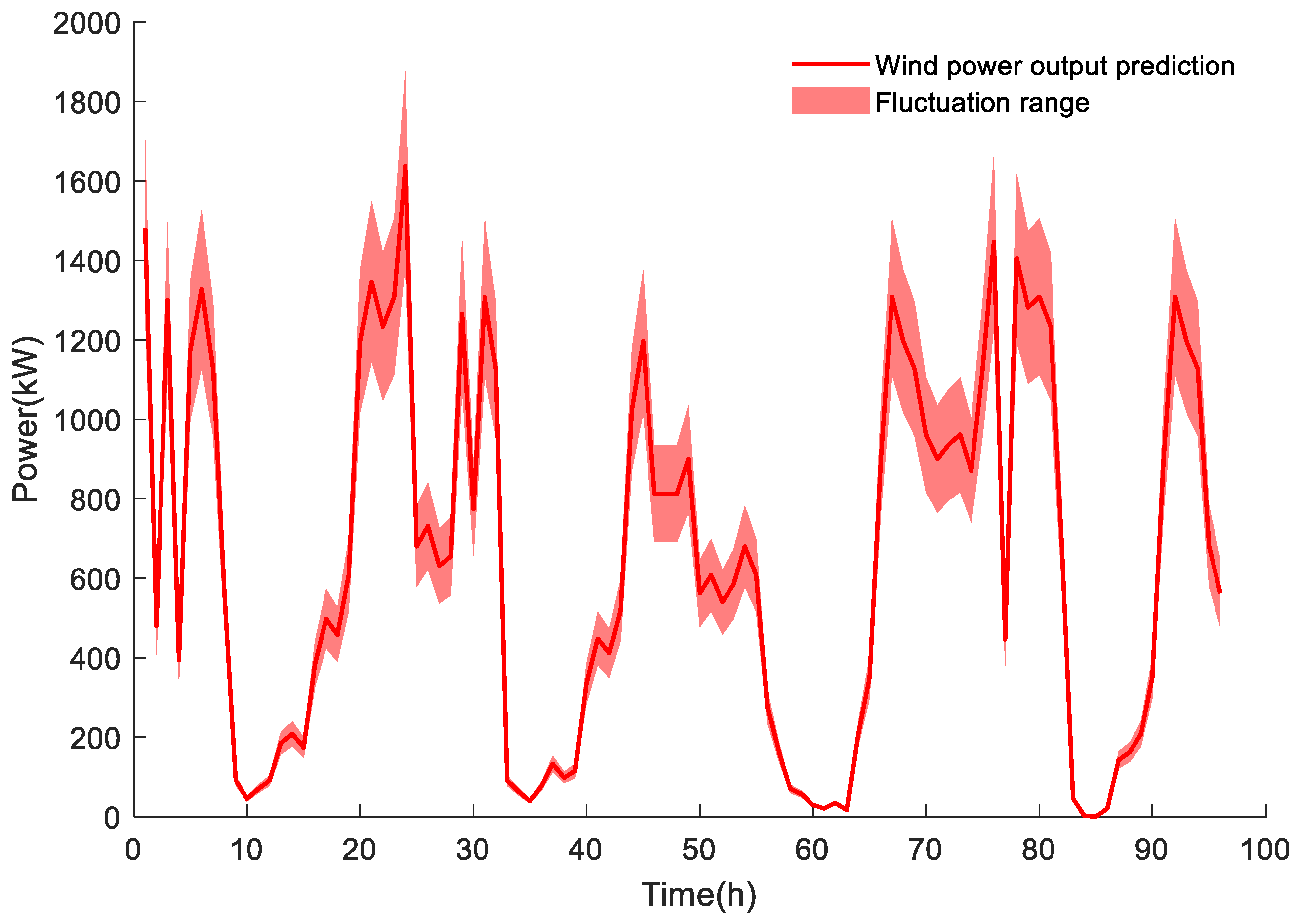
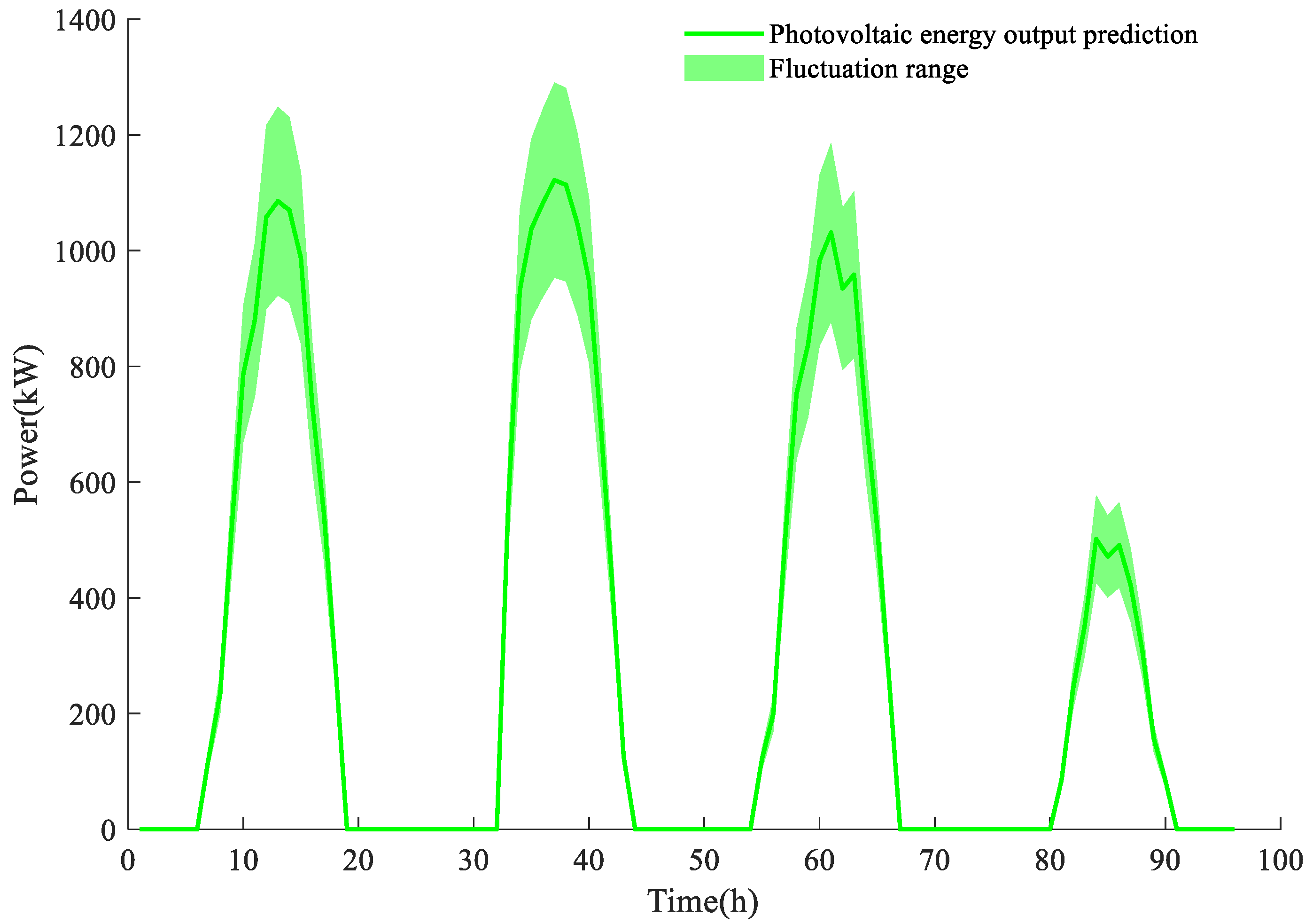
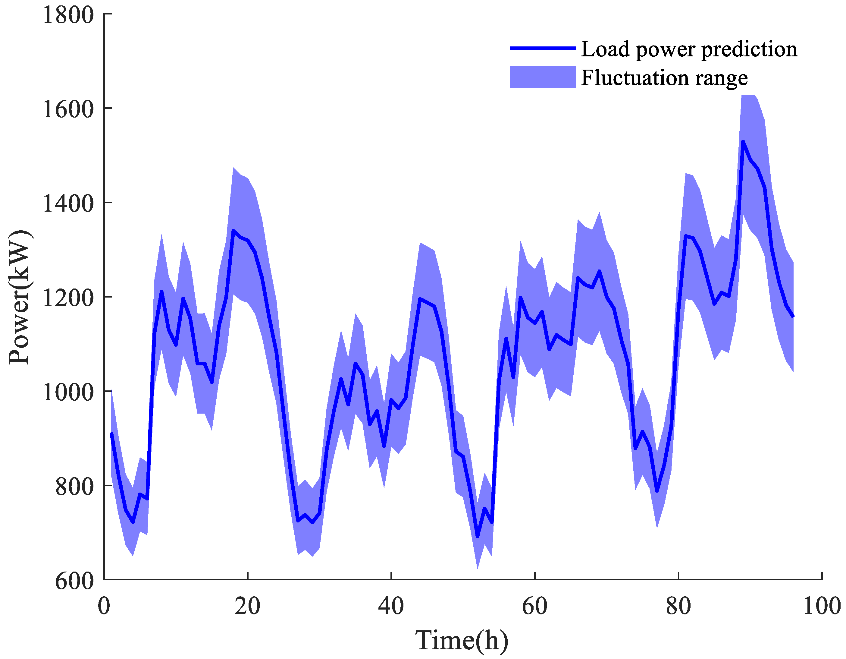
The inherent uncertainties associated with renewable generation and load forecasting are modeled using box uncertainty sets, which provide a computationally tractable yet robust framework for handling worst-case scenarios. Based on statistical analysis of historical forecast errors in the region [30], the fluctuation ranges are set at ±15% for wind and photovoltaic power outputs and ±10% for load demand. The forecasted power outputs with their uncertainty bounds for wind power, photovoltaic generation, and electrical load across the four typical days are illustrated in Figure 2, Figure 3 and Figure 4, respectively.

Key economic and technical parameters for the equipment are drawn from reference [30]. The model’s key sets, variables, and parameters, as summarized in Table 2, are instantiated with the following values. The economic and technical parameters are provided in Table 3, Table 4 and Table 5, respectively. The tiered carbon trading mechanism is configured with a base price of 0.3 CNY/kg and a price growth rate of 25%. To isolate and quantify the impact of the proposed mechanisms, four distinct configuration schemes are designed and compared:

Scheme 1: Baseline. Optimal configuration without considering any carbon trading mechanism.

Scheme 2: Basic Carbon Trading. Optimal configuration incorporating a basic carbon trading mechanism (fixed price).

Scheme 3: Tiered Carbon Trading. Optimal configuration under a tiered carbon trading mechanism (price increases with emission levels).

Scheme 4: Proposed Method. Optimal configuration integrating both tiered carbon trading and incentive-based demand response (DR).

Table 3. Economic parameters of related equipment.

Device Name	Capitalized Cost/(CNY/kW) or (CNY/m3)	Maintenance/ Investment Costs	Maintenance Costs/(CNY/kW) or (CNY/m3)
Fan-driven generator	6655	0.01	66.55
Photovoltaic	6075	0.02	121.5
Gas generator	690	0.02	13.8
Storage battery	1400	0.02	28
Electrolyzer	2000	0.04	80
Methanation equipment	3000	0.05	150
Carbon capture equipment	0.92	0.4	0.37
Hydrogen storage equipment	7.76	0.02	0.12
Carbon storage equipment	7.76	0.02	0.12

Table 3. Economic parameters of related equipment.

Device Name	Capitalized Cost/(CNY/kW) or (CNY/m3)	Maintenance/ Investment Costs	Maintenance Costs/(CNY/kW) or (CNY/m3)
Fan-driven generator	6655	0.01	66.55
Photovoltaic	6075	0.02	121.5
Gas generator	690	0.02	13.8
Storage battery	1400	0.02	28
Electrolyzer	2000	0.04	80
Methanation equipment	3000	0.05	150
Carbon capture equipment	0.92	0.4	0.37
Hydrogen storage equipment	7.76	0.02	0.12
Carbon storage equipment	7.76	0.02	0.12

Table 4. Other economic parameters.

Class	Time Quantum	Price
Electricity price (CNY/kW·h)	01:00–08:00	0.382
	08:00–12:00
	16:00–19:00	0.54
	22:00–24:00
	12:00–16:00	0.922
	19:00–22:00

Table 4. Other economic parameters.

Class	Time Quantum	Price
Electricity price (CNY/kW·h)	01:00–08:00	0.382
	08:00–12:00
	16:00–19:00	0.54
	22:00–24:00
	12:00–16:00	0.922
	19:00–22:00

Table 5. Technical parameters of related equipment.

Parameter	Value
${\eta }^{\mathrm{CCS}}$	0.65
$e_{\mathrm{GT}}$(m3/kW·h)	0.707
${\lambda }_{{\mathrm{co}}_2}$(kW·h/m3)	0.1937
${\lambda }_{{\mathrm{H}}_2}$(kW·h/m3)	4.2
${\lambda }_{{\mathrm{CH}}_4}$(kW·h/m3)	0.3
$c_{{\mathrm{CH}}_4,t}$(CNY/m3)	2.5

Table 5. Technical parameters of related equipment.

Parameter	Value
${\eta }^{\mathrm{CCS}}$	0.65
$e_{\mathrm{GT}}$(m3/kW·h)	0.707
${\lambda }_{{\mathrm{co}}_2}$(kW·h/m3)	0.1937
${\lambda }_{{\mathrm{H}}_2}$(kW·h/m3)	4.2
${\lambda }_{{\mathrm{CH}}_4}$(kW·h/m3)	0.3
$c_{{\mathrm{CH}}_4,t}$(CNY/m3)	2.5

5.2. Analysis of Microgrid Planning and Operation Results

The optimal capacity configuration and corresponding cost calculations for the four schemes are detailed in

Table 6. Microgrid capacity configuration results for four schemes.

Scheme	1	2	3	4
Wind turbine (kW)	1638	1689	1831	1830
Photovoltaic (kW)	1365	1401	1602	1535
Gas generator (kW)	344	339	323	263
Electrolyzer (kW)	0	26	135	27
Methanation equipment (kW)	0	2	4	2
CCS (kW)	0	4	6	5
Hydrogen storage equipment (m3)	0	71	150	81
Carbon storage equipment (m3)	0	43	142	45

and

Table 7. Cost calculation results of four microgrid schemes.

Scheme	1	2	3	4
Investment maintenance cost (CNY 10,000)	280.87	289.22	321.80	311.18
Gas cost (CNY 10,000)	64.42	57.92	31.64	34.16
DR compensation cost (CNY 10,000)	0	0	0	1.78
Penalty cost (CNY 10,000)	30.39	31.72	33.83	34.45
Carbon trading cost (CNY 10,000)	0	12.60	15.34	16.26
Purchase cost of electricity from superior units (CNY 10,000)	54.92	52.79	51.34	44.48
Total cost (CNY 10,000)	430.59	444.25	453.96	439.08
Carbon emissions (ton)	1518.57	1424.49	1128.25	1034.18
Carbon capture (ton)	0	9.98	72.45	16.92

.

5.2.1. Impact of Tiered Carbon Pricing

The results demonstrate the significant influence of carbon pricing mechanisms. In Scheme 1 (baseline, without carbon trading), the installed capacities for wind turbines (WTs) and photovoltaics (PVs) are 1638 kW and 1365 kW, respectively. The absence of a carbon cost penalty results in greater reliance on the gas turbine (GT), with a capacity of 344 kW. The CCS and P2G coupling remains largely inactive due to its economic infeasibility under these conditions.

Introducing a basic carbon trading mechanism in Scheme 2 drives a discernible shift towards decarbonization. WT and PV capacities increase by 3.11% and 2.64%, respectively, while the GT capacity is reduced by 1.45%. The imposition of a carbon cost renders the CCS-P2G system economically viable, evidenced by the installation of a 26 kW electrolyzer. This configuration leads to a significant reduction in carbon emissions—approximately 94 tons lower than Scheme 1, albeit at a higher total cost due to the newly incurred carbon expenses.

Scheme 3, incorporating a tiered carbon pricing mechanism, further amplifies these trends. The escalating cost associated with higher emission tiers provides a stronger incentive for a more aggressive low-carbon strategy. The electrolyzer capacity experiences a substantial increase of 109 kW compared to Scheme 2, thereby enhancing the CCS-P2G coupling and enabling the capture and utilization of an additional 72.45 tons of CO₂. Consequently, carbon emissions are further reduced, validating the superior effectiveness of the tiered mechanism in promoting deep decarbonization.

5.2.2. Impact of DR

The introduction of incentive-based DR in Scheme 4, the proposed method, yields the most balanced and economically efficient outcome. By enabling load shifting from peak to off-peak periods, DR flattens the load curve and improves its alignment with renewable generation profiles. This reduces the need for peak capacity provided by the GT and power purchases from the main grid. As a result, Scheme 4 achieves the lowest total cost among all scenarios, at CNY 4,390,800, which is 3.28% lower than Scheme 3. Simultaneously, it maintains a low-carbon profile, with emissions reduced by a further 94.07 tons compared to Scheme 3. This demonstrates that DR acts as a critical flexibility resource, delivering a “win–win” outcome of enhanced economics and environmental performance. The annual power generation breakdown for each scheme, illustrated in Figure 5, clearly shows the reduced reliance on gas and grid power in Scheme 4, underscoring the synergistic effect of DR with renewable energy integration.

5.2.3. Comparative Analysis of DR and CCS-P2G: Mechanisms, Costs, and System Impacts

The configuration results of Scheme 4, particularly the reduced capacity of the gas turbine (GT), can be attributed to the fundamental differences between Demand Response (DR) and CCS-P2G. A comparative analysis of their operational mechanisms and associated costs clarifies their distinct roles in microgrid planning.

Operational Mechanism: Active Demand-Side Management vs. Passive Supply-Side Processing

Demand Response (DR) functions as an active demand-side management tool. It addresses the “supply-demand mismatch” at its source by reshaping the load profile to better align with renewable generation. By shifting flexible loads from peak to off-peak periods, DR directly reduces the system’s reliance on peak-capacity generators and expensive power purchases.

CCS-P2G (Carbon Capture and Power-to-Gas) operates as a passive supply-side processing technology. It serves as an “end-of-pipe” treatment for carbon emissions after combustion and a utilization pathway for surplus electricity. This two-stage process is inherently energy-intensive: the carbon capture system consumes significant power, while the P2G conversion suffers from substantial efficiency losses (typically 30–50%). Consequently, operating CCS-P2G introduces a considerable new load to the system, potentially increasing net energy consumption and operational complexity.

Cost Structure: Low OpEx Incentives vs. High CapEx/OpEx Investment

The cost of DR is predominantly operational expenditure (OpEx) in the form of incentive payments to users. This is a transparent, controllable cost that is typically far lower than the marginal cost of peak electricity or carbon trading fees, making DR an effective cost saver.

In contrast, CCS-P2G entails high capital expenditure (CapEx) for equipment (electrolyzers, reactors, capture units) and significant OpEx due to its massive energy consumption. It functions as a net energy consumer and represents a high-cost mitigation pathway.

Synthesis: Explaining the Optimal Configuration in Scheme 4

The integration of DR in Scheme 4 enables a more economical and efficient system configuration. By flattening the load curve, DR diminishes the need for gas turbines to meet peak demand, leading to the observed reduction in GT capacity. This load-shifting also enhances renewable energy self-consumption, reducing both curtailment and the necessity for large-scale, energy-intensive CCS-P2G facilities to manage excess generation or emissions.

Practical Implication: This analysis yields a critical guideline for planners: under budget constraints, priority should be given to developing demand-side flexibility resources (e.g., DR, customer-side storage) over investing in capital-intensive supply-side technologies like CCS-P2G. Operationally, system dispatchers should prioritize dispatching DR as a virtual generation resource before activating more expensive options, marking a shift from a “source-follows-load” paradigm to an advanced “source-load interaction” model.

5.3. Impact of Uncertainty on Microgrids

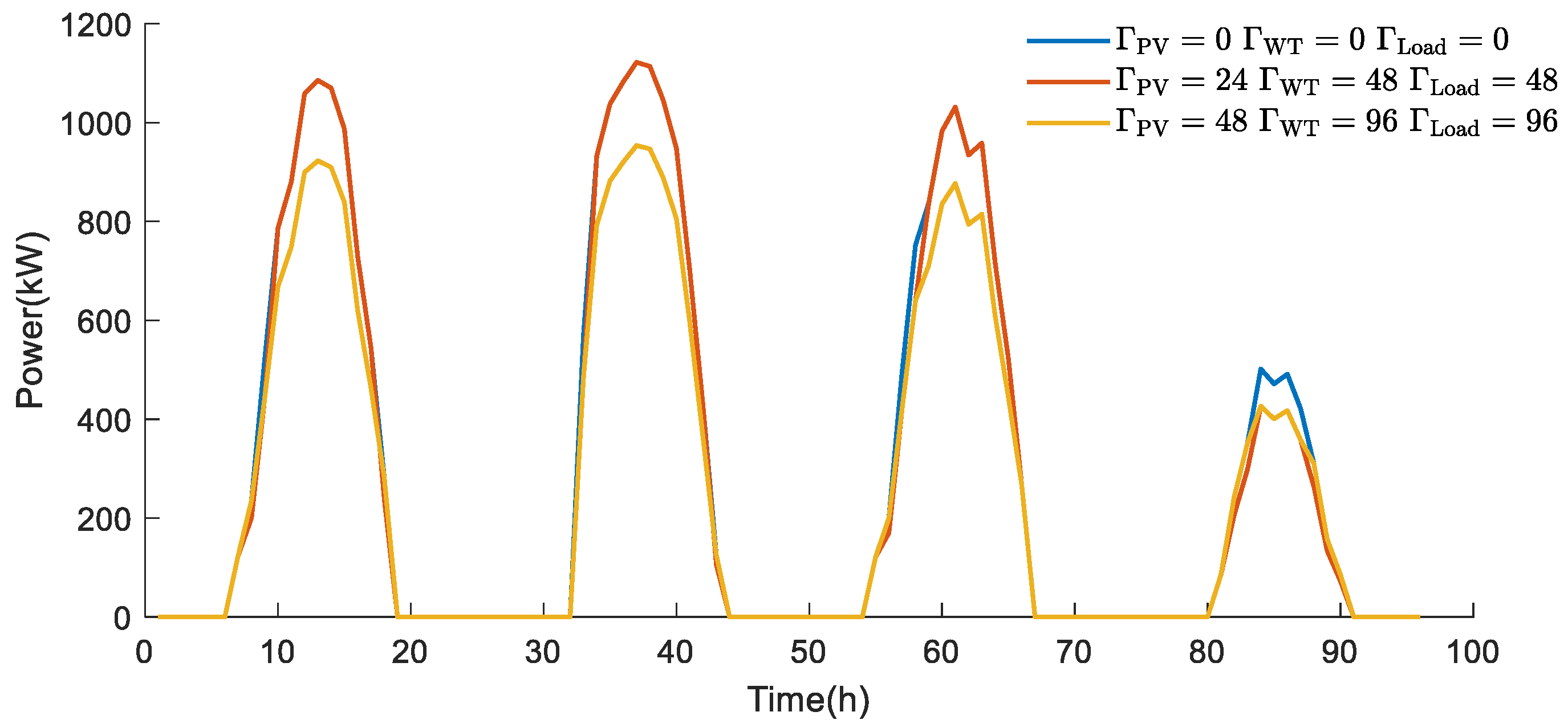
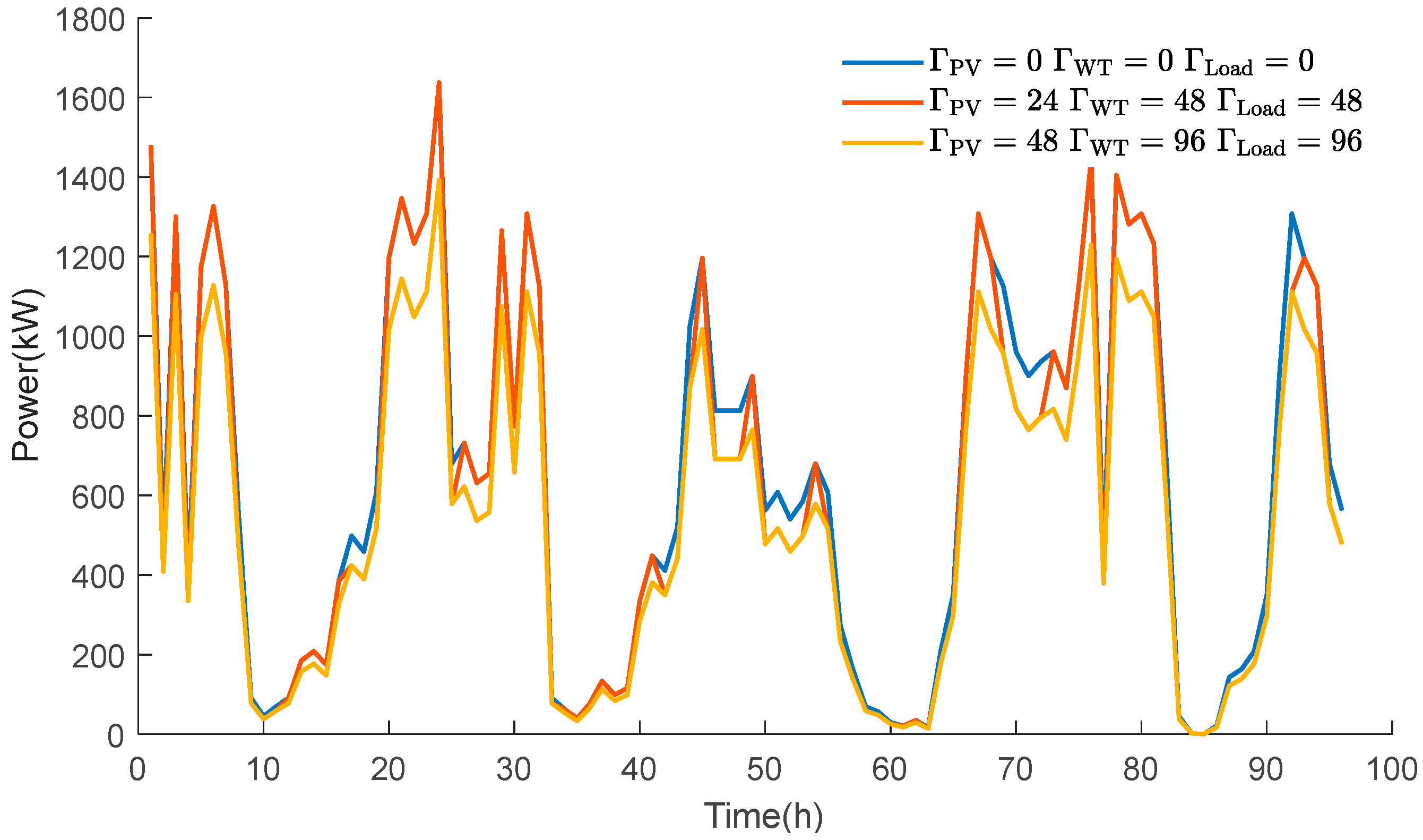
To show the influence of uncertainty, three different types of uncertain parameter ratios are set up. In Figure 6 and Figure 7, ${\Gamma }_{\mathrm{P}\mathrm{V}}$, ${\Gamma }_{\mathrm{W}\mathrm{T}}$, and ${\Gamma }_{\mathrm{L}\mathrm{o}\mathrm{a}\mathrm{d}}$ show the output under different conditions of ${\Gamma }_{\mathrm{P}\mathrm{V}}$, ${\Gamma }_{\mathrm{W}\mathrm{T}}$, and ${\Gamma }_{\mathrm{L}\mathrm{o}\mathrm{a}\mathrm{d}}$ with uncertain parameters. The values of uncertain parameters are set to 0, 24, or 48, and the values of certain parameters are set to 0, 48, or 96, respectively.

The adverse scenarios for wind and solar power generation under different uncertain parameter settings, as shown in Figure 6 and Figure 7, reveal that the output of wind and solar equipment reaches the lower $B_{\mathrm{W}\mathrm{T},t}^{-}$ bound $B_{\mathrm{P}\mathrm{V},t}^{-}$ of $B_{\mathrm{e},\mathrm{Load},t}^{+}$, the interval under adverse conditions $P_{\mathrm{W}\mathrm{T},t},P_{\mathrm{P}\mathrm{V},t}$, while the load $P_{\mathrm{e},\mathrm{Load},t}$ reaches the upper ${\Gamma }_{\mathrm{P}\mathrm{V}}=24$ bound ${\Gamma }_{\mathrm{W}\mathrm{T}},{\Gamma }_{\mathrm{L}\mathrm{o}\mathrm{a}\mathrm{d}}=48$ of the interval. The worst-case scenario occurs when the 0–1 variables in the uncertain parameters are all equal to 1, at which point the lower or upper bound is taken for all times. That is, when the target function value increases, the wind and solar load output values also increase.

Three sets of scenarios are designed to investigate the influence of uncertain parameters on the results.

Scenario 1: ${\Gamma }_{\mathrm{P}\mathrm{V}}=0,{\Gamma }_{\mathrm{W}\mathrm{T}}=0,{\Gamma }_{\mathrm{L}\mathrm{o}\mathrm{a}\mathrm{d}}=0$;

Scenario 2: ${\Gamma }_{\mathrm{P}\mathrm{V}}=24,{\Gamma }_{\mathrm{W}\mathrm{T}}=48,{\Gamma }_{\mathrm{L}\mathrm{o}\mathrm{a}\mathrm{d}}=48$;

Scenario 3: ${\Gamma }_{\mathrm{P}\mathrm{V}}=48,{\Gamma }_{\mathrm{W}\mathrm{T}}=96,{\Gamma }_{\mathrm{L}\mathrm{o}\mathrm{a}\mathrm{d}}=96$.

A comparison of the capacity optimization results under different uncertainty parameter scenarios is provided in

Table 8. Comparison of capacity optimization results under different uncertain parameter scenarios.

Uncertainty Adjustment Parameters	Scenario 1	Scenario 2	Scenario 3
Wind turbine (kW)	1830	1830	1555
Photovoltaic (kW)	1535	1535	1535
Gas generator (kW)	263	489	505
Electrolyzer (kW)	27	27	0
Methanation equipment (kW)	2	2	0
CCS (kW)	4	5	4
Hydrogen storage equipment (m3)	150	150	150
Carbon storage equipment (m3)	150	150	150

.

The corresponding cost optimization results are compared in

Table 9. Comparison of cost optimization results in different uncertain parameter scenarios.

Uncertainty Adjustment Parameters	Scenario 1	Scenario 2	Scenario 3
Investment maintenance cost (CNY 10,000)	311.18	313.54	287.67
Gas cost (CNY 10,000)	34.07	67.34	95.05
DR compensation cost (CNY 10,000)	1.78	1.93	1.98
Penalty cost (CNY 10,000)	34.45	31.02	29.71
Carbon trading cost (CNY 10,000)	16.25	30.10	43.95
Purchase cost of electricity from superior units (CNY 10,000)	44.93	70.19	103.28
Total cost (CNY 10,000)	439.10	510.22	557.69
Carbon emissions (ton)	1034.84	1760.63	2580.19

.

Compared to the two tables above, the wind and solar power capacity has not decreased, but the annual power generation has reduced. Moreover, due to changes in wind and solar output and load demand, wind and solar power cannot effectively fill the gap left by load consumption, leading to gas costs increasing by CNY 332,700 and CNY 609,800 in Scenarios 2 and 3 compared to Scenario 1. The gas configuration capacity increased by 226 kW and 242 kW, respectively, and the amount of electricity purchased from higher levels increased by CNY 252,600 and CNY 583,500. Due to cost constraints, the CCS and P2G coupling phase did not increase capacity to enhance internal circulation, resulting in microgrid internal carbon emissions increasing by 725.79 tons and 1535.34 tons in Scenarios 2 and 3 compared to Scenario 1, with total costs increasing by CNY 711,200 and CNY 1,185,900, respectively. This shows that as the uncertain adjustment parameter values gradually increase, robustness improves, and the configuration scenarios become more conservative, leading to an increase in both carbon emissions and total costs.

Interpretation of Uncertainty Deviation Patterns

As illustrated in Figure 6, the uncertainty in wind power forecast output is distributed relatively uniformly throughout the day during spring and autumn. In contrast, the uncertainty increases significantly during winter nights. This pattern aligns with the meteorological characteristics of the region, where wind speed variability is inherently higher during winter nights. The error bars quantitatively reveal a critical insight: while the absolute fluctuating power during nightly low-output periods may be lower than during daytime hours, the relative fluctuation rate is considerably higher. This highlights a period of high volatility relative to the expected generation level, which is a crucial risk factor for system balancing.

Figure 7 demonstrates that the uncertainty band for photovoltaic output is the narrowest around noon during summer. This indicates that solar radiation intensity forecasts are most accurate during peak insolation hours when the sun’s position is most predictable. Conversely, the uncertainty band widens considerably during sunrise and sunset periods. This phenomenon underscores that forecast model errors increase relatively under low irradiance conditions, where factors like cloud cover and atmospheric attenuation have a proportionally greater impact on the predicted output.

The analysis of Figure 6 shows that load forecast uncertainty is most pronounced—indicated by the longest error bars—during morning and evening peak demand periods. This directly reflects the concentrated yet stochastic nature of user behavior during these times, as activities like appliance usage, heating, or cooling are aggregated and can vary significantly. In comparison, load forecasting during nighttime hours is considerably more stable. This stability arises from a lower overall demand level and more predictable base-load consumption patterns, resulting in a narrower uncertainty band.

5.4. Sensitivity Analysis

The uncertainty ranges for wind/solar (±15%) and load (±10%) are based on historical forecast errors in Northwest China [30]. The carbon trading base price (0.3 CNY/kg) and growth rate (25%) align with tiered carbon trading mechanisms in virtual power plants [11], reflecting realistic policy scenarios.

To validate the robustness of the proposed two-stage robust optimization model and to investigate the impact of key parameters on the optimal configuration, a comprehensive sensitivity analysis is conducted. This section examines the influence of variations in the carbon trading mechanism, uncertainty levels of renewable energy and load, and the participation rate of demand response. The baseline scenario (S0) for comparison is the optimal configuration from Scheme 4 in the case study.

5.4.1. Analysis Setup and Scenario Design

Three critical parameter sets are selected for the sensitivity analysis, each varied within a plausible range to create distinct scenarios:

Carbon Trading Mechanism (Scenarios A1, S0, A2): This evaluates the impact of carbon policy stringency.

A1 (Lenient Policy): Base carbon price = 0.2 CNY/kg, price growth rate = 20%.

S0 (Baseline Policy): Base carbon price = 0.3 CNY/kg, price growth rate = 25%.

A2 (Stringent Policy): Base carbon price = 0.5 CNY/kg, price growth rate = 30%.

Uncertainty Levels (Scenarios B1, S0, B2): This assesses the effect of forecast accuracy for renewables and load.

B1 (Low Uncertainty): RE fluctuation range = ±10%, load fluctuation range = ±5%.

S0 (Baseline Uncertainty): RE fluctuation range = ±15%, load fluctuation range = ±10%.

B2 (High Uncertainty): RE fluctuation range = ±20%, load fluctuation range = ±15%.

Demand Response Participation (Scenarios C1, S0, C2): This examines the value of load-side flexibility.

C1 (Low DR): DR participation rate = 10%.

S0 (Baseline DR): DR participation rate = 20%.

C2 (High DR): DR participation rate = 30%.

For each scenario, the two-stage robust optimization model is resolved using the C&CG algorithm to obtain the new optimal capacity configuration, total annual cost, and carbon emissions.

5.4.2. Results and Discussion

The optimization results for all sensitivity scenarios are summarized in

Table 10. Sensitivity analysis results for different parameter scenarios.

Scenario	Wind (kW)	PV (kW)	GT (kW)	Electrolyzer (kW)	Total Cost (CNY 104)	Carbon Emissions (ton)
S0 (Baseline)	1830	1535	263	27	439.08	1034.18
A1 (Lenient Carbon)	1750 (−4.4%)	1480 (−3.6%)	310 (+17.9%)	15 (−44.4%)	428.50 (−2.4%)	1250.50 (+20.9%)
A2 (Stringent Carbon)	1950 (+6.6%)	1650 (+7.5%)	200 (−23.9%)	45 (+66.7%)	455.20 (+3.7%)	850.75 (−17.7%)
B1 (Low Uncertainty)	1750 (−4.4%)	1500 (−2.3%)	280 (+6.5%)	20 (−25.9%)	425.80 (−3.0%)	1100.25 (+6.4%)
B2 (High Uncertainty)	1900 (+3.8%)	1580 (+2.9%)	350 (+33.1%)	30 (+11.1%)	465.50 (+6.0%)	1350.60 (+30.6%)
C1 (Low DR)	1850 (+1.1%)	1550 (+1.0%)	290 (+10.3%)	25 (−7.4%)	445.50 (+1.5%)	1150.30 (+11.2%)
C2 (High DR)	1800 (−1.6%)	1510 (−1.6%)	240 (−8.7%)	32 (+18.5%)	432.00 (−1.6%)	950.45 (−8.1%)

, with percentage changes calculated relative to the baseline S0. The optimization results for all sensitivity scenarios are summarized in Table 10.

Impact of Carbon Trading Mechanism

The results from Scenarios A1 and A2 demonstrate that the carbon trading price is a powerful driver for decarbonization. Under a more stringent policy (A2), the capacity of wind and PV increases significantly (+6.6% and +7.5%, respectively) to replace carbon-intensive generation. Consequently, the gas turbine (GT) capacity is reduced by 23.9%. The P2G system, particularly the electrolyzer, sees a dramatic 66.7% increase in capacity, as it provides a critical sink for excess renewable electricity and utilizes captured CO₂. This configuration shift leads to a substantial 17.7% reduction in carbon emissions.

However, this environmental benefit comes at a 3.7% increase in total cost, primarily due to higher investment in renewables and P2G, as well as increased carbon trading costs per unit of remaining emission. Conversely, a lenient policy (A1) leads to a cheaper but higher-carbon system.

Although the carbon price growth rate is a key parameter, the model’s results exhibit moderate-to-high sensitivity to it, rather than being extremely sensitive. This implies that while variations in the growth rate influence the optimal capacity configuration and total cost, the proposed model remains robust across a plausible range of carbon policy stringency.

Impact of Uncertainty Levels

The analysis of uncertainty (Scenarios B1 and B2) reveals that forecast inaccuracy directly compromises both the economic and environmental performance of the microgrid. In the high-uncertainty scenario (B2), the robust optimization model adopts a conservative strategy, increasing the capacity of the dispatchable GT by 33.1% to ensure reliability under the worst-case scenario. While RE capacity also increases slightly to harness more energy, the system becomes more carbon-intensive, leading to a 30.6% surge in emissions and a 6.0% increase in total cost. This underscores that improving the forecast accuracy of renewable generation and load is not merely an operational issue but a critical factor in reducing the cost of achieving low-carbon goals.

Impact of Demand Response Participation

The DR analysis (Scenarios C1 and C2) highlights its role as a key flexibility resource. With higher DR participation (C2), the load profile can be shaped to better match renewable generation. This reduces the need for peak capacity, evidenced by the 8.7% reduction in GT capacity. The improved alignment between supply and demand also allows for a slight reduction in wind and PV capacity (−1.6%) while increasing the utilization of the P2G system. The overall effect is a “win–win” outcome: total cost decreases by 1.6%, and carbon emissions fall by 8.1%. This confirms that incentivizing DR participation is a cost-effective strategy for enhancing both the economy and low-carbon operation of the microgrid.

5.5. Discussion: Comparison with Other Uncertainty Optimization Methods

To further evaluate the performance of our method and outline future research directions, this subsection discusses and compares it with two other mainstream uncertainty optimization methods.

5.5.1. Comparison with Distributionally Robust Optimization (DRO)

DRO methods do not assume that uncertain parameters follow a specific precise distribution. Instead, they assume the true distribution lies within an “ambiguity set” (often constructed using Wasserstein distance or φ-divergence) centered on the empirical distribution. It seeks the optimal solution under the worst-case probability distribution within this set, philosophically “optimizing the expectation of the worst-case distribution.” DRO strikes a balance between stochastic programming and traditional RO. Compared to the box-based RO used here, DRO is typically less conservative because it utilizes the distribution information of historical data, not just the fluctuation intervals.

5.5.2. Comparison with Two-Stage Stochastic Programming (SP)

Stochastic programming typically requires generating many scenarios with explicit probabilities (e.g., through Monte Carlo simulation or historical data clustering) and optimizes the expected total cost across these scenarios. Stochastic programming methods often yield more economically efficient plans because they optimize average performance. However, they highly depend on the accuracy of the input probabilities; if the actual situation deviates significantly from the assumed probability distribution, the plan’s performance can deteriorate sharply.

6. Patent

Jilin Provincial Department of Science and Technology Science and Technology Development Plan Project “Research and Application of Key Technologies for a Wind-Solar Complementary Intelligent Agricultural Drip Irrigation System Based on IoT + Cloud Architecture” (Project No.: 20220203112SF).

References

1. Ren, D.; Liu, Z.; Gao, F.; Gao, C.; Song, G. Electrothermal coordinated operation optimization of park integrated energy system considering carbon trading mechanism and demand response. Therm. Power Gener. 2022, 51, 119–130. [Google Scholar] [CrossRef]
2. Tan, Y.; Meegahapola, L.; Muttaqi, K.M. A review of technical challenges in planning and operation of remote area power supply systems. Renew. Sustain. Energy Rev. 2014, 38, 876–889. [Google Scholar] [CrossRef]
3. Zhou, X.; Zhao, Q.; Zhang, Y.; Sun, L. Integrated energy production unit: An innovative concept and design for energy transition toward low-carbon development. CSEE J. Power Energy Syst. 2021, 7, 1133–1139. [Google Scholar] [CrossRef]
4. Li, J.; Liu, P.; Li, Z. Optimal design of a hybrid renewable energy system with grid connection and comparison of techno-economic performances with an off-grid system: A case study of West China. Comput. Chem. Eng. 2022, 159, 107657. [Google Scholar] [CrossRef]
5. Zhang, Y.; Sun, H.; Tan, J.; Li, Z.; Hou, W.; Guo, Y. Capacity configuration optimization of multi-energy system integrating wind turbine/photovoltaic/hydrogen/battery. Energy 2022, 252, 124046. [Google Scholar] [CrossRef]
6. Zuo, G.; Guo, H.; Lin, W.; Yu, Y.; Lv, Y. Optimal configuration of microgrid considering low-carbon hydrogen production. Electr. Power Automat. Equip. 2023, 43, 9–18. [Google Scholar] [CrossRef]
7. Bailera, M.; Peña, B.; Lisbona, P.; Romeo, L.M. Decision-making methodology for managing photovoltaic surplus electricity through Power to Gas: Combined heat and power in urban buildings. Appl. Energy 2018, 228, 1032–1045. [Google Scholar] [CrossRef]
8. Zhang, K.; Gao, C.; Zhang, G.; Xie, T.; Li, H. Electricity and heat sharing strategy of regional comprehensive energy multi-microgrid based on double-layer game. Energy 2024, 293, 130655. [Google Scholar] [CrossRef]
9. Cui, Y.; Zhou, H.; Zhong, W.; Li, H.; Zhao, Y. Low-carbon scheduling of power system with wind power considering uncertainty of both source and load sides. Electr. Power Automat. Equip. 2020, 40, 85–93. [Google Scholar] [CrossRef]
10. Zhao, Z.; Li, X. Low-carbon economic dispatch based on ladder carbon trading virtual powerplant considering carbon capture power plant and Power-to-Gas. Power Gener. Technol. 2023, 44, 769–780. [Google Scholar]
11. Ma, Y.; Meng, R.; Wei, B.; Li, T. Two-stage robust optimal scheduling of a microgrid with a stepped carbon trading mechanism. Power Syst. Protect. Control 2023, 51, 22–33. [Google Scholar] [CrossRef]
12. Jin, S.; Mao, Z.; Li, H. Economic operation optimization of smart micro grid considering the uncertainty. Control Theory Appl. 2018, 35, 1357–1370. [Google Scholar]
13. Peng, C.; Zhang, J.; Chen, L.; Sun, H. Source-load-storage coordinated optimal scheduling of microgrid considering differential demand response. Electr. Power Automat. Equip. 2020, 40, 1–7. [Google Scholar] [CrossRef]
14. Jiang, Z.; Xiang, Y.; Tan, Z.; Guo, Y.; Wang, Y.; Zhou, K. Optimal operation strategy for virtual power plant considering regulation market and external demand response. Electr. Power 2023, 56, 147–155+163. [Google Scholar]
15. Rezaei, S.; Ghasemi, A. Stochastic scheduling of resilient interconnected energy hubs considering peer-to-peer energy trading and energy storages. J. Energy Storage 2022, 50, 104665. [Google Scholar] [CrossRef]
16. Wei, B.; Han, X.; Li, W.; Guo, L.; Yu, H. Multi-time scale stochastic optimal dispatch for AC/DC hybrid microgrid incorporating multi-scenario analysis. High Volt. Eng. 2020, 46, 2359–2369. [Google Scholar] [CrossRef]
17. Prathapaneni, D.R.; Detroja, K.P. An integrated framework for optimal planning and operation schedule of microgrid under uncertainty. Sustain. Energy Grids Netw. 2019, 19, 100232. [Google Scholar] [CrossRef]
18. Su, W.; Wang, J.; Roh, J. Stochastic energy scheduling in microgrids with intermittent renewable energy resources. IEEE Trans. Smart Grid 2014, 5, 1876–1883. [Google Scholar] [CrossRef]
19. Mehrjerdi, H. Simultaneous load leveling and voltage profile improvement in distribution networks by optimal battery storage planning. Energy 2019, 181, 916–926. [Google Scholar] [CrossRef]
20. Tan, J.; Wu, Q.; Zhang, M.; Wei, W.; Liu, F.; Pan, B. Chance-constrained energy and multi-type reserves scheduling exploiting flexibility from combined power and heat units and heat pumps. Energy 2021, 233, 121176. [Google Scholar] [CrossRef]
21. Deng, P.; Liu, Y.; Bi, Y.; Yang, P. Survey on robust linear optimization. Control Decis. 2009, 24, 1121–1125+1131. [Google Scholar] [CrossRef]
22. Liu, Y.; Guo, L.; Wang, C. Economic dispatch of microgrid based on two stage robust optimization. Proc. CSEE 2018, 38, 4013–4022+4307. [Google Scholar] [CrossRef]
23. Wang, L.; Dong, H.; Lin, J.; Zeng, M. Multi-objective optimal scheduling model with IGDT method of integrated energy system considering ladder-type carbon trading mechanism. Int. J. Electr. Power Energy Syst. 2022, 143, 108386. [Google Scholar] [CrossRef]
24. Wei, Z.; Zhang, S.; Sun, G.; Xu, X.; Chen, S.; Chen, S. Carbon trading based low-carbon economic operation for integrated electricity and natural gas energy system. Autom. Electr. Power Syst. 2016, 40, 9–16. [Google Scholar]
25. Chen, W.; Wu, Z. Carbon emission permit allocation and trading. J. Tsinghua Univ. (Sci. Technol.) 1998, 12, 16–19+23. [Google Scholar] [CrossRef]
26. Kirschen, D.S.; Strbac, G.; Cumperayot, P.; Mendes, D.D.P. Factoring the elasticity of demand in electricity prices. IEEE Trans. Power Syst. 2000, 15, 612–617. [Google Scholar] [CrossRef]
27. Federal Energy Regulatory Commission Staff Team. 2012 Assessment of Demand Response and Advanced Metering Staff Report; Federal Energy Regulatory Commission: Washington, DC, USA, 2012. [Google Scholar]
28. Shui, Y.; Liu, J.; Gao, H.; Qiu, G.; Xu, W.; Gou, J. Two-stage distributed robust cooperative dispatch for integrated elcctricity and natural gas energy systems considering uncertainty of wind power. Autom. Electr. Power Syst. 2018, 42, 43–50+75. [Google Scholar]
29. Mulvey, J.; Vanderbei, R.; Zenios, S. Robust Optimization of Large-Scale Systems. Oper. Res. 1995, 43, 264–281. [Google Scholar] [CrossRef]
30. Zhang, X.; Zhang, Y. Environment-friendly and economical scheduling optimization for integrated energy system considering power-to-gas technology and carbon capture power plant. J. Clean. Prod. 2020, 276, 123348. [Google Scholar] [CrossRef]
Figure 1. Microgrid structure.
Symmetry 17 01999 g001
Figure 2. Wind power forecasts output and its fluctuations.
Symmetry 17 01999 g002
Figure 3. Photovoltaic forecast output and its fluctuations.
Symmetry 17 01999 g003
Figure 4. Load forecast and its fluctuations.
Symmetry 17 01999 g004
Figure 5. Comparison of annual power generation under different schemes.
Symmetry 17 01999 g005
Figure 6. Deviation between typical daily wind power output and forecast value in four seasons.
Symmetry 17 01999 g006
Figure 7. Deviation between typical daily PV output and forecast value in four seasons.
Symmetry 17 01999 g007