Settlement Prediction of Preloading Method Based on SSA-BP Neural Network with Consideration of Asymmetric Settlement Behavior

Abstract

This study focuses on the East Channel Project (Xiang’an South Road—Airport Expressway Section). The project is in the South Port Harbor Bay area. The area has highly complex and asymmetrical geology. Construction faces multiple challenges: tight schedule, overlapping pipeline operations, and large-scale foundation treatment needs. To tackle these, the project uses the plastic drainage board surcharge preloading method for ground improvement. This technique needs continuous settlement deformation monitoring. The monitoring aims to spot potential asymmetric trends and fix the best unloading time. Traditional settlement prediction methods have limits. So, this study develops an intelligent prediction model (SSA-BP). It combines the Sparrow Search Algorithm (SSA) with the BP neural network. The model uses SSA’s strong global search ability to optimize the BP network’s initial weights and thresholds. This effectively avoids local minima and improves prediction stability. Comparative experiments with other optimization algorithms (Particle Swarm Optimization PSO, Grey Wolf Optimizer GWO, and Differential Evolution DE) show that the SSA-BP model has better convergence accuracy and robustness. Field monitoring data validation indicates the model’s prediction error is stably between −3.4% and 3.2%. It surpasses traditional methods like the three-point and hyperbolic methods. The study’s key innovation is introducing an asymmetry-aware view. It analyzes settlement’s morphological evolution and predictability under surcharge preloading. The SSA-BP model can identify both symmetric and asymmetric deformation patterns well. It offers a new computational tool to understand asymmetry breaking in geotechnical systems. Moreover, the model can accurately predict settlement behavior in real time. This provides dynamic construction decision-making guidance and effective cost control. This research shows that intelligent algorithms have great potential. They can reveal complex geotechnical systems’ inherent laws and promote foundation engineering’s intelligentization.

1. Introduction

The Xidong Road project (also known as the Binhai East Avenue-Airport Expressway) is situated in Xiang’an District, Xiamen City, Fujian Province, China (as is shown in Figure 1). It begins at Binhai East Avenue to the north, crosses the Nangang Sea via a bridge, continues onto Dadeng Island, and terminates at the Xunku Interchange. The route generally follows a northwest-southeast orientation. The plastic drainage board preloading method is widely employed in infrastructure development—including highways, railways, airport runways, and port facilities—particularly in soft soil areas. As the cross-sea segment of the Xidong Road project traverses a land reclamation zone characterized by weak foundation conditions, the plastic drainage board preloading method has been adopted for ground improvement in this section.

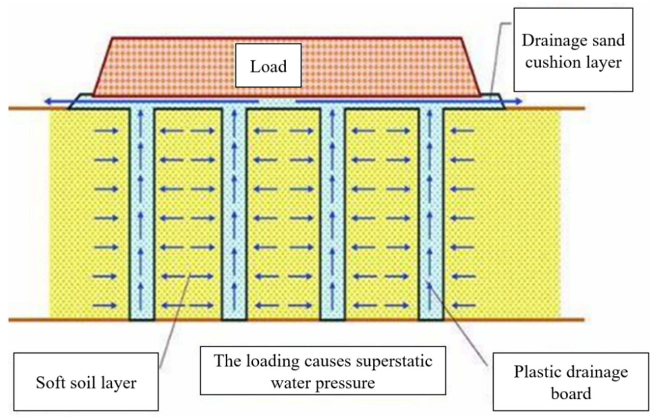
The plastic drainage board preloading method is extensively applied in diverse construction contexts (as is shown in Figure 2). Scholars like Li [1] have probed its role in water conservancy embankments. She [2] has assessed its efficacy in a Fuzhou factory scenario, and He [3] has examined its utility in tropical water-rich soft soil zones in Sri Lanka’s southern railway project. In practice, this method efficiently boosts soil drainage consolidation across scenarios, with strong construction adaptability and environmental advantages [4,5,6]. As technology advances, its integration with other reinforcement approaches, such as vacuum preloading and composite drainage systems, has further uplifted soil reinforcement efficiency and better managed settlement issues in engineering construction on soft soil foundations [7].

Recent years have witnessed the emergence of novel materials and technologies, such as composite plastic drainage boards [8], reinforced drainage boards [9], and multi-layer drainage systems [10]. These innovative drainage boards excel in drainage efficiency and longevity, handling complex soil conditions with ease. Vacuum preloading technology, which expedites drainage via negative pressure and shortens construction time, has also been adopted in certain projects [11,12,13].

A crucial aspect of the plastic drainage board preloading method is determining the optimal unloading timing. Premature unloading can lead to uneven settlement, while delayed unloading can slow down project progress. Accurately forecasting settlement patterns and planning unloading timing are of great practical significance. Currently, classical settlement prediction methods such as the three-point and hyperbolic methods are widely used.

However, these empirical approaches rely on idealized assumptions regarding soil homogeneity and symmetric consolidation behavior, limiting their applicability under complex preloading and drainage conditions. In recent years, data-driven models such as BP neural networks have shown the ability to capture complex nonlinear relationships among soil deformation, load history, and settlement development. These models can simulate nonlinear behaviors like soil creep and plastic deformation with higher precision than empirical methods. Nevertheless, conventional BP networks still face several challenges, including low convergence efficiency, susceptibility to local optima, and lack of adaptability to asymmetric settlement behavior, which often occurs in practical soft soil engineering. To address these limitations, this study develops an asymmetry-aware hybrid model that combines the Sparrow Search Algorithm (SSA) with the BP neural network. The SSA component provides strong global search and self-adaptive exploration capabilities, enabling the BP network to escape local minima and better represent asymmetric consolidation patterns. Beyond accuracy improvement, the proposed SSA-BP framework further offers decision-guidance outputs that support preload scheduling and monitoring frequency optimization. Comparative analysis with classic and existing AI-based models verifies the enhanced convergence speed, predictive accuracy, and engineering applicability of the proposed approach.

2. Sparrow Search Algorithm Theory

2.1. Research Status of Sparrow Search Optimization Algorithm

Optimization algorithms have significantly enhanced computational efficiency and problem-solving capabilities for complex issues. Li [14] introduced a novel intelligent model (the beluga whale optimization-based–kernel extreme learning machine model, BWO-KELM) for predicting surface settlement (Ss), trained on 148 monitoring data points with eight features from three tunnel projects. Liao [15] developed an intelligent monitoring system incorporating a BP neural network to accurately predict settlement in high-fill subgrade, validated through on-site experiments. Hu [16] proposed a mechanism-driven intelligent settlement prediction method (MISPM), integrating settlement mechanisms and construction-induced movements to derive informative indirect features. Kovačević [17] conducted a comprehensive evaluation of multiple machine learning techniques—including multiple linear regression, Multigene Genetic Programming (MGGP), ensemble regression trees, Gaussian Process Regression (GPR), Support Vector Regression (SVR), and neural networks—for predicting the interfacial bond strength of fiber-reinforced polymer (FRP) concrete. The Sparrow Search Algorithm (SSA), known for its simplicity and effectiveness, has gained widespread application across multiple domains, especially in engineering optimization, machine learning, data mining, and image processing [18].

In engineering optimization, SSA is extensively used in structural optimization and mechanical design. Gao [19] leveraged SSA to optimize bridge structural design, achieving weight reduction and an enhanced load-bearing capacity. By imitating sparrow population search strategies, SSA effectively avoids local optima and boosts optimization efficiency [20]. In machine learning, SSA is applied to hyperparameter optimization, feature selection, and classification. Zhang [21] demonstrated that SSA improves classification accuracy in SVM parameter optimization. Zhou [22] utilized SSA for feature selection, surpassing traditional methods. SSA has also made significant strides in image processing, particularly in image segmentation and enhancement. Shi [23] enhanced image segmentation accuracy through SSA-optimized algorithms, while Zhang [24] showed SSA’s effectiveness in image denoising while preserving details.

Furthermore, SSA excels in other fields, especially in autonomous driving in dynamic environments. Liu [25] proposed a dynamic path planning method based on SSA, improving planning efficiency and safety. In resource scheduling for industrial production and computer networks, Khaleel [26] found SSA -based job scheduling reduces completion time and improves resource utilization. Abdulhammed [27] applied SSA to optimize cloud computing task scheduling and resource allocation. Jia [28] proposed the UAV launch parameter prediction method based on the SSA-BP model, and the superiority of SSA-BP for launch parameter prediction is comprehensively evaluated based on MAE, MAPE, and RMSE evaluation methods. To achieve accurate strength prediction and mix proportion optimization for slag–cement-stabilized soil, Zhang [29] used SSA to optimize initial network parameters, constructing an SSA-BP model that effectively enhances convergence speed and generalization capability. Gao [30] introduced a machine learning predictive control method and constructed a BP neural network prediction model based on the sparrow optimization algorithm (SSA-BP).

2.2. Principles of Sparrow Search Optimization Algorithm

The Sparrow Search Algorithm (SSA) draws inspiration from the foraging and predator avoidance behaviors of sparrow populations in nature. The core idea of this algorithm is to simulate the behavior patterns of sparrow populations and combine mechanisms such as discovering food, avoiding danger, and detecting warnings to conduct global optimization searches. The design inspiration for the Sparrow Search Algorithm comes from how sparrow populations collaborate and self-adjust to forage and survive in the most optimal way when facing danger [31].

Assuming that, in a sparrow population, sparrows play two roles, discoverers searching for food and participants in the population, the algorithm process is as follows [32]:

Establish a population of n sparrows, where d represents the dimensionality of the problem corresponding to the sparrow’s solution.

$$X=\left[\begin{array}{cccc}{x}_{1,1}& x_{1,2}& \dots & x_{1,d}\\ x_{2,1}& x_{2,2}& \dots & x_{2,d}\\ ⋮& ⋮& ⋮& ⋮\\ x_{n,1}& x_{n,2}& \dots & x_{n,d}\end{array}\right]$$

(1)

Choose an appropriate fitness function f to represent the size of each sparrow’s hunting ability, expressed as

$$F_X=\left[\begin{array}{cccc}f\left(\left[x_{1,1}\right.\right.& x_{1,2}& \dots & \left.\left.x_{1,d}\right]\right)\\ f\left(\left[x_{2,1}\right.\right.& x_{2,2}& \dots & \left.\left.x_{2,d}\right]\right)\\ & ⋮& & \\ & ⋮& & \\ f\left(\left[x_{n,1}\right.\right.& x_{n,2}& \dots & \left.\left.x_{n,d}\right]\right)\end{array}\right]$$

(2)

Update on the location of sparrows that have discovered food:

$$X_{i,j}^{t+1}=\left\{\begin{array}{cc}{X}_{i,j}^t\cdot \exp \left(-{\displaystyle \frac{i}{\alpha \cdot {\mathrm{iter}}_{max}}}\right)& \mathrm{if}{R}_2<ST\\ X_{i,j}^t+QL& \mathrm{if}{R}_2\ge ST\end{array}\right.$$

(3)

$t$—Sparrow search iteration number;

$j$—Problem dimension;

${\mathrm{iter}}_{max}$—Algorithm setting constants;

$X_{i,j}^t$—Indicate the position information of the i-th sparrow in the j-th dimension at time t;

$X_{i,j}^{t+1}$—Representing the position information of the i-th sparrow in the j-th dimension at time t+1;

$\alpha$—Random numbers between [0, 1];

$R_2$—Alert threshold, with a value range of [0, 1];

$ST$—Safe value, with a value range of [0.5, 1];

$Q$—Random numbers that follow a normal distribution, with a value range of [0, 1];

$L$—A matrix of 1 × d.

When $R_2$ < ST, the predatory sparrows do not pose a threat from predators and can search and hunt within a safe area; if $R_2\ge$ ST, it indicates that sparrows are in danger, and all sparrows will fly out of the current area to a relatively safe area for searching and foraging. Discoverers will randomly move to other locations according to a normal distribution.

Update the location of the joiner:

$$X_{i,j}^{t+1}=\left\{\begin{array}{ccc}Q\cdot \exp \left({\displaystyle \frac{X_{\mathrm{worst}}-X_{i,j}^t}{i^2}}\right)& \mathrm{if}& i>{\displaystyle \frac{n}{2}}\\ X_P^{t+1}+\left|X_{i,j}^t-X_p^{t+1}\right|\cdot A^{+}\cdot L& \mathrm{otherwise}& \end{array}\right.$$

(4)

$X_p$—The best location for discoverers;

$X_{worst}$—The worst location for discoverers;

$A$—Representing a 1 × d matrix with elements of 1 or −1, $A^{+}=A^T{\left(A{A}^T\right)}^{-1}$.

When i > n/2, sparrows with lower adaptability need to obtain more food. In other cases, sparrows are located near their optimal position and randomly search for a new location nearby.

Reconnaissance and early warning behavior:

During the process of sparrows searching for food, some sparrows will be responsible for vigilance. In case of danger, all sparrows will exhibit anti-hunting behavior, drop their current food, and move to a new location.

$$X_{i,j}^{t+1}=\left\{\begin{array}{cc}{X}_{\mathrm{best}}^t+\beta \cdot \left|X_{i,j}^t-X_{\mathrm{best}}^t\right|& \mathrm{if}{f}_i>f_{\mathrm{g}}\\ & \\ X_{i,j}^t+K\cdot \left({\displaystyle \frac{X_{i,j}^t-X_{\mathrm{worst}}^t}{\left(f_i-f_w\right)+\epsilon }}\right)& \mathrm{if}{f}_i=f_g\end{array}\right.$$

(5)

$\beta$—Random numbers that conform to the standard normal distribution;

$K$—Uniform random numbers between [−1, 1];

$f_i$—Sparrow fitness value;

$f_{\mathrm{g}}$—The fitness value of sparrows in their optimal position;

$f_w$—The fitness value of sparrows in the worst position.

When $f_i=f_g$, at this moment, the sparrow is in a dangerous position, stay away from the worst sparrow. When $f_i>f_{\mathrm{g}}$, sparrows are easily attacked by predators, so they will move towards the optimal sparrow position.

3. Construction of SSA-BP Model

The backpropagation (BP) neural network is a multi-layer feedforward neural network, which is one of the most classic and widely used models in the field of neural networks, suitable for tasks such as classification, regression, and pattern recognition. The BP neural network consists of an input layer, a hidden layer, and an output layer. It updates weights through forward and backward propagation to predict data. But it is prone to getting stuck in local optima, and for deep networks, backpropagation requires a large amount of computation. Therefore, the powerful global search capability of the Sparrow Search Algorithm can be utilized to improve the overall prediction accuracy of neural networks [33]. The specific process is as follows, and the process diagram is shown in Figure 3.

The number of hidden layers plays a critical role in determining the predictive performance of the SSA-BP neural network. An excessive number of hidden layers may result in overfitting, whereas too few layers can hinder the model’s ability to capture complex relationships between input and output variables, thereby reducing prediction accuracy. Consequently, the network’s predictive capability strongly depends on the appropriate selection of hidden layers. The optimal number of hidden layer neurons can be estimated using the following empirical formula [34]:

$$\begin{array}{c}l<n-1\\ l<\sqrt{\left(m+n\right)}+a\\ l={\log }_{2}n\end{array}$$

(6)

n—Number of input layer nodes;

$m$—Number of input nodes;

$l$—Number of hidden layer nodes;

$a$—A constant between [0, 10].

This formula can determine a rough range for the number of hidden layers. In this paper, the hidden layer range is set to [3,15], and the root mean square error of the training set under each hidden layer is calculated separately. Finally, the hidden layer with the smallest root mean square error (RSME) is selected as the optimal value.

3.1. SSA-BP Model Evaluation Indicators

The evaluation of predictive performance can be measured using the following indicators [35].

Sum of squared errors SSE:

$$SSE=\sum _{\mathrm{i}=1}^{\mathrm{n}}{\left(y_i-{\widehat{y}}_i\right)}^2$$

(7)

Mean absolute error MAE:

$$MAE={\displaystyle \frac{1}{n}}\sum _{i=1}^n\left|{\widehat{y}}_i-y_i\right|$$

(8)

Mean absolute percent error MAPE:

$$MAPE={\displaystyle \frac{100\%}{n}}\sum _{i=1}^n\left|{\displaystyle \frac{{\widehat{y}}_i-y_i}{y_i}}\right|$$

(9)

Mean squared error MSE:

$$MSE={\displaystyle \frac{1}{n}}\sum _{\mathrm{i}=1}^{\mathrm{n}}{\left(y_i-{\widehat{y}}_i\right)}^2$$

(10)

Root mean square error RMSE:

$$RMSE=\sqrt{{\displaystyle \frac{1}{n}}\sum _{\mathrm{i}=1}^{\mathrm{n}}{\left(y_i-{\widehat{y}}_i\right)}^2}$$

(11)

Correlation coefficient R:

$$R=\sqrt{1-{\displaystyle \frac{\sum _{\mathrm{i}=1}^{\mathrm{n}}{\left(y_i-{\widehat{y}}_i\right)}^2}{\sum _{\mathrm{i}=1}^{\mathrm{n}}{\left(y_i-\overline{y}\right)}^2}}}$$

(12)

Coefficient of determination R²:

$$R^2=1-{\displaystyle \frac{\sum _{\mathrm{i}=1}^{\mathrm{n}}{\left(y_i-{\widehat{y}}_i\right)}^2}{\sum _{\mathrm{i}=1}^{\mathrm{n}}{\left(y_i-\overline{y}\right)}^2}}$$

(13)

3.2. Algorithm Excellence Test

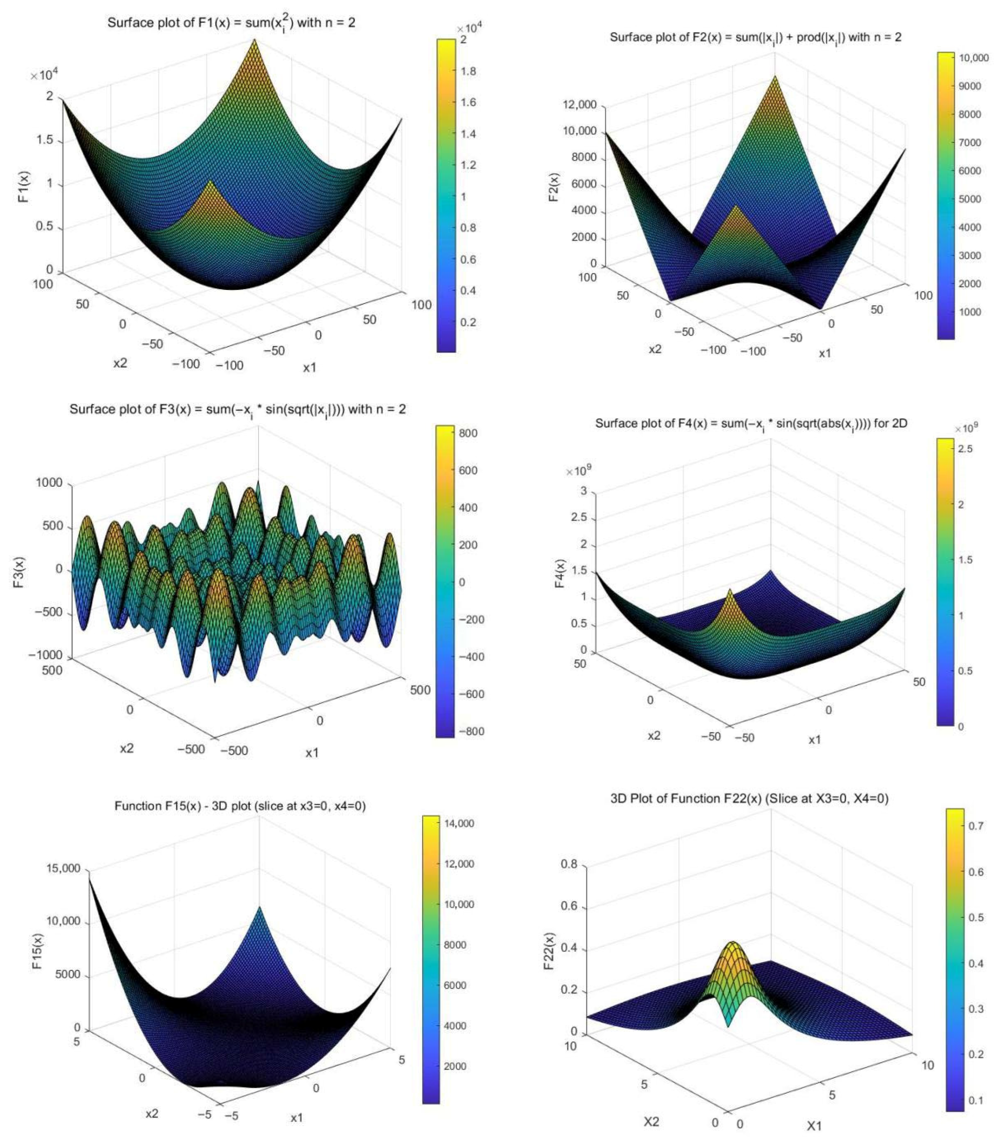
In optimization algorithms, benchmark test functions are commonly employed to evaluate algorithmic performance and robustness. In this study, four representative algorithms—Particle Swarm Optimization (PSO), Grey Wolf Optimization (GWO), Differential Evolution (DE), and Sparrow Search Algorithm (SSA)—were selected for comparative analysis. The parameter settings for each algorithm are listed in

Table 1. Algorithm parameter setting.

Algorithm	PSO	DE	GWO	SSA
Parameters	c1 = 2 c2 = 2 Wmin = 0.2 Wmax = 0.9	CR = 0.2 Fmin = 0.2 Fmax = 0.8	a = (2→0)	ST = 0.8 PD = 0.2 SD = 0.2

, and the selected benchmark test functions are summarized in

Table 2. Test function.

Test Function	Dimension	Interval	Minimum Value
$F_1(x)={\displaystyle \sum _{i=1}^n}{x}_i^2$	30	[−100, 100]	0
$F_2(x)={\displaystyle \sum _{i=1}^n}\left|x_i\right|+{\displaystyle \prod _{i=1}^n}\left|x_i\right|$	30	[−100, 100]	0
$F_3(x)={\displaystyle \sum _{i=1}^n}-x_i\mathrm{s}\mathrm{i}\mathrm{n}\left(\sqrt{\left|x_i\right|}\right)$	30	[−500, 500]	−418.98 × dim
$F_4\left(x\right)={\displaystyle \frac{\pi }{n}}\left\{10\sin \pi y_1+{\displaystyle \sum _{i=1}^{n-1}}{(y_i-1)}^2\left[1+10{sin}^2(\pi y_{i+1})\right]+{(y_n-1)}^2\right\}$ $+{\displaystyle \sum _{i=1}^n}u(x_i,10,100,4)y_i=1+{\displaystyle \frac{x_i+1}{4}}$ $u(x_i,a,k,m)=\left\{\begin{array}{c}k{(x_i-a)}^m{x}_i>a\\ 0-a<x_i<a\\ k{({-x}_i-a)}^m{x}_i<-a\end{array}\right.$	30	[−50, 50]	0
$F_{15}(x)={\displaystyle \sum _{i=1}^{11}}{\left(a_i-{\displaystyle \frac{x_1(b_i^2+b_1{x}_2)}{b_i^2+b_1{x}_3+x_4}}\right)}^2$	4	[−5, 5]	0
$F_{22}(x)={\displaystyle \sum _{i=1}^7}{\left[\left(X-a_i\right){\left(X-a_i\right)}^T+c_i\right]}^{-1}$	4	[0, 10]	−10.40

.

The above function graphs were created using Matlab 2023 (as is shown in Figure 4):

The above algorithm was used to solve it through matlab, and the results are shown in

Table 3. Algorithm solution results.

F	Indicators/Algorithms	PSO	DE	GWO	SSA
	Best	8.93 × 10−6	5.55 × 10−14	6.31 × 10−28	0
	Worst	8.36 × 10−4	4.46 × 104	4.66 × 10−25	1.37 × 10−67
F1	Ave	1.63 × 10−4	3.31 × 103	5.25 × 10−26	4.58 × 10−69
	Std	2.13 × 10−4	1.07 × 104	1.13 × 10−25	2.51 × 10−68
	Rank	3	4	2	1
	Best	4.10 × 10−4	5.61	1.47 × 10−16	0
	Worst	0.27	3.71 × 1013	1.61 × 10−15	3.45 × 10−40
F2	Ave	0.04	1.28 × 1012	6.19 × 10−16	1.15 × 10−41
	Std	5.50 × 10−2	6.77 × 1012	3.56 × 10−16	6.30 × 10−41
	Rank	3	4	2	1
	Best	−7203.72	−12566	−10562	−1.26 × 104
	Worst	−2664.29	−6671.64	−8506.23	−9.50 × 103
F3	Ave	−5937.33	−10130.9	−9321.52	−1.06 × 104
	Std	1187.28	1920.468	1570.104	2.61 × 103
	Rank	4	2	3	1
	Best	5.13 × 10−7	3.55 × 10−3	6.06 × 10−3	1.57 × 10−32
	Worst	0.114	9.25 × 10−2	6.53 × 10−2	4.18 × 10−8
F4	Ave	3.90 × 10−2	2.40 × 10−2	2.25 × 10−2	2.15 × 10−9
	Std	2.10 × 10−2	1.86 × 10−2	1.45 × 10−2	8.19 × 10−9
	Rank	4	3	2	1
	Best	4.10 × 10−3	5.608	1.47 × 10−16	0
	Worst	2.71 × 10−1	3.71 × 1013	1.61 × 10−15	3.45 × 10−40
F15	Ave	4.03 × 10−2	1.28 × 1012	6.19 × 10−16	1.15 × 10−41
	Std	5.51 × 10−2	6.77 × 1012	3.56 × 10−16	6.30 × 10−41
	Rank	3	4	2	1
	Best	−10.402	−6.431	−10.4	−10.402
	Worst	−2.752	−0.528	−5.09	−5.088
F22	Ave	−8.587	−1.759	−9.34	−9.871
	Std	3.105	1.362	2.162	1.622
	Rank	3	4	2	1

.

In the test results, Best denotes the optimal value, Worst denotes the worst value, Ave represents the mean value, and Std indicates the standard deviation. As shown in the results, the Sparrow Search Algorithm (SSA) demonstrates outstanding performance across all evaluation metrics. It achieves superior results in terms of best, worst, average, and standard deviation values compared with other algorithms, confirming its strong optimization capability and high stability.

3.3. Comparison of SSA-BP Vertical Settlement Prediction

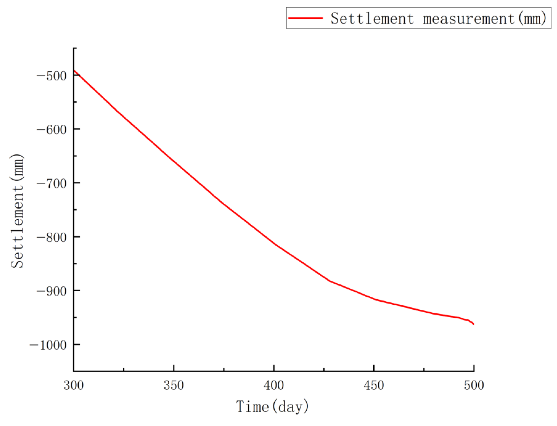
The vertical displacement monitoring points located between chainages K6 + 510 and K7 + 235.362 of the Xidong Road project were selected for this study. A total of 200 data records collected after the stabilization of settlement deformation were used as the research samples. The monitoring data from the first four days were employed as cyclic inputs to predict the vertical settlement on the fifth day, generating a total of 196 predictive samples, as illustrated in Figure 5. To evaluate the predictive performance of the model, the first 176 samples were used for training, while the remaining 20 samples were reserved for testing.

Vertical displacement serves as a critical indicator for assessing construction safety and ensuring overall construction quality. As shown in the figure above, the final settlement at the monitoring point reaches 962.9 mm, indicating that the settlement process has entered a stable stage. During this period, the subgrade is not affected by external construction activities or other disturbances, and the settlement values exhibit a gradually convergent trend. The proposed SSA-BP neural network model can effectively predict the settlement evolution of the soil under these stable conditions.

Basic parameter determination in SSA-BP neural network:

• ① BP neural network parameter setting

In the BP neural network, the learning rate was set to 0.1, and the number of training iterations was fixed at 1000. The purelin function was used as the activation function in the output layer, while the tansig function was applied in the hidden layer. The network adopted the learngdm function as its learning rule and the traingdx function as its training algorithm. The model configuration consisted of four input parameters, one output parameter, and fourteen hidden neurons.

• ② Basic parameter settings for Sparrow Search Algorithm

According to the computational requirements of this study, the basic parameters of the Sparrow Search Algorithm (SSA) were determined based on the characteristics of the dataset and the network structure. The specific parameter settings are as follows: the number of iterations was set to 30, the sparrow population size to 30, and the warning threshold to 0.8, with 20% of the population designated as alert individuals and 80% as discoverers.

• ③ Train and predict

The settlement data was inputted into a model with the same BP neural network structure to optimize the initial network weights and thresholds and then compare them with the BP neural network optimized by genetic algorithm.

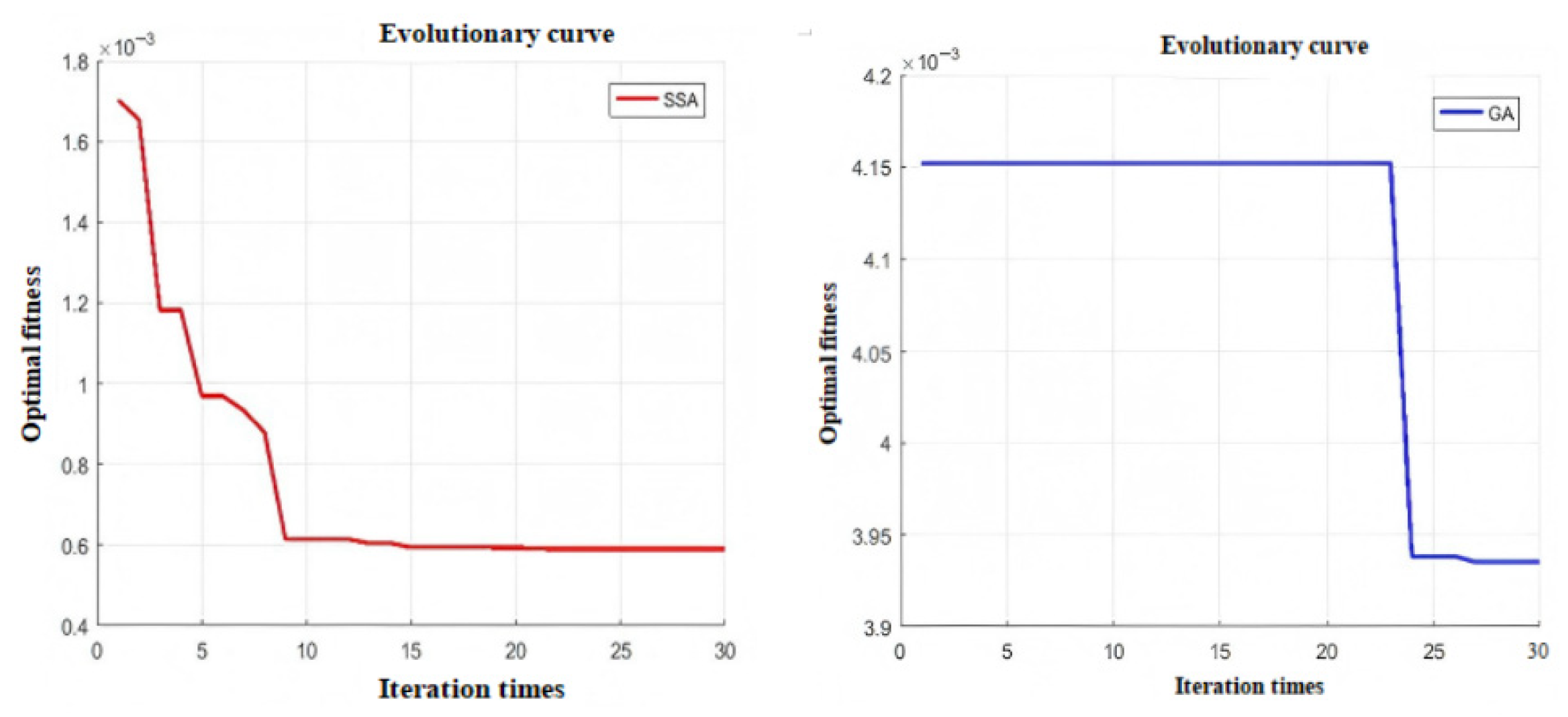
As is shown in Figure 6, the genetic algorithm (GA) requires more iterations to converge compared with the Sparrow Search Algorithm (SSA). The use of SSA for optimizing the initial weights and thresholds of the neural network significantly improves computational efficiency and convergence speed. The optimal fitness value obtained by SSA is approximately 6 × 10⁻⁴, whereas that achieved by GA is only about 3.94 × 10⁻³. Therefore, the initial weights and thresholds optimized by SSA yield higher network prediction accuracy in this study. The corresponding prediction results are presented in

Table 4. Prediction results of different neural networks.

Period	Actuality (mm)	BP Neural Networks			GA-BP Neural Networks			SSA-BP Neural Networks
		Estimate	Error	Percentage	Estimate	Error	Percentage	Estimate	Error	Percentage
1	−943.8	−914.2	29.6	−3.1%	−917.5	26.3	−2.8%	−919.6	24.2	−2.6%
2	−944.0	−915.2	28.8	−3.1%	−918.2	25.8	−2.7%	−920.5	23.5	−2.5%
3	−945	−916.2	28.8	−3.0%	−919.4	25.6	−2.7%	−921.7	23.3	−2.5%
4	−945.8	−917.5	28.3	−3.0%	−920.5	25.3	−2.7%	−922.8	23	−2.4%
5	−946.2	−918.6	27.6	−2.9%	−921.6	24.6	−2.6%	−924.0	22.2	−2.3%
6	−946.8	−919.5	27.3	−2.9%	−922.4	24.4	−2.6%	−925.2	21.6	−2.3%
7	−947.7	−920.5	27.2	−2.9%	−923.6	24.1	−2.5%	−927.1	20.6	−2.2%
8	−948	−921.5	26.5	−2.8%	−924.1	23.9	−2.5%	−929.1	18.9	−2.0%
9	−948.6	−922.4	25.4	−2.8%	−924.5	24.1	−2.5%	−930.5	18.1	−1.9%
10	−949.2	−923.8	25.4	−2.7%	−925.1	24.1	−2.5%	−931.6	17.6	−1.9%
11	−949.8	−924.9	24.9	−2.6%	−926.2	23.6	−2.5%	−933.2	16.6	−1.7%
12	−950.2	−926.0	24.2	−2.5%	−927.3	22.9	−2.4%	−935.1	15.1	−1.6%
13	−951.1	−927.2	23.9	−2.5%	−929.2	21.9	−2.3%	−937.2	13.9	−1.5%
14	−952.3	−928.6	23.7	−2.5%	−931.2	21.1	−2.2%	−939.5	12.8	−1.3%
15	−953.9	−929.3	24.6	−2.6%	−933.2	20.7	−2.2%	−941.0	12.9	−1.4%
16	−954.6	−930.2	24.4	−2.6%	−934.5	20.1	−2.1%	−943.2	11.4	−1.2%
17	−954.5	−931.5	23	−2.4%	−935.6	18.9	−2.0%	−945.5	9	−0.9%
18	−957.6	−932.5	25.1	−2.6%	−936.1	21.5	−2.2%	−947.8	9.8	−1.0%
19	−959.3	−933.6	25.7	−2.7%	−937.2	22.1	−2.3%	−949.2	10.1	−1.1%
20	−962.9	−934.5	28.4	−2.9%	−938.6	24.3	−2.5%	−951.3	11.6	−1.2%

.

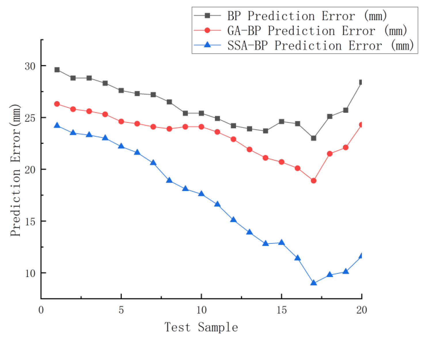
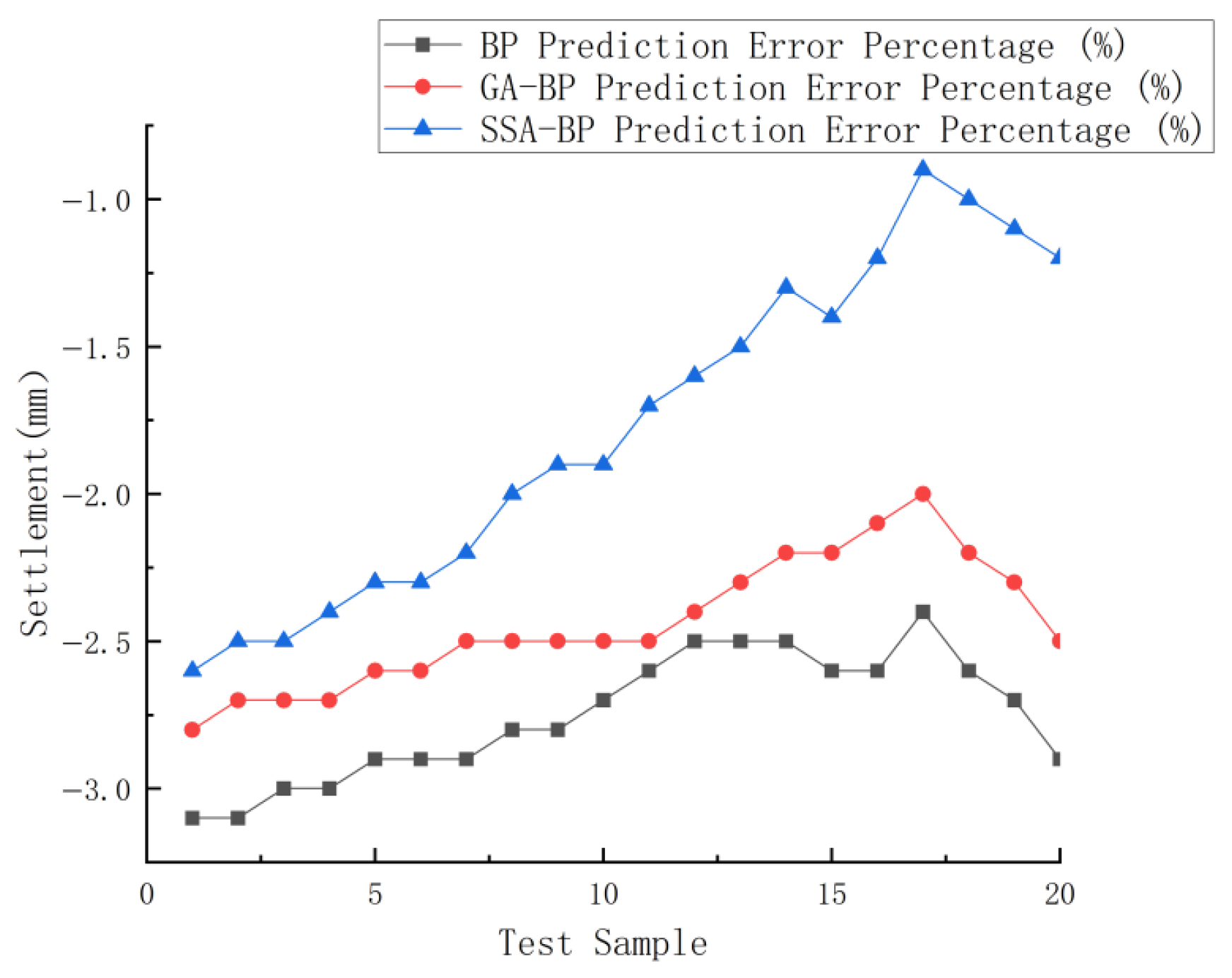
As illustrated in Figure 7, Figure 8 and Figure 9, the prediction accuracy of the SSA-BP neural network model is significantly higher than that of the BP and GA-BP neural networks, and its predictions align more closely with the measured values. The prediction error of the SSA-BP model remains generally within 20 mm, whereas the errors of the BP and GA-BP models are consistently above this threshold, indicating lower accuracy. From the perspective of error percentage, the SSA-BP model maintains prediction errors within 2.5%, while both the GA-BP and BP models exhibit higher deviations, confirming that the SSA-BP model optimized by the Sparrow Search Algorithm achieves a superior predictive performance.

As shown in

Table 5. Evaluation index values for different models.

Evaluation	BP	GA-BP	SSA-BP
SSE	13,781.8	10,904.0	6158.7
MAE	26.18	23.27	16.81
MSE	689.1	545.2	307.9
RMSE	26.25	23.35	17.55
MAPE	2.75%	2.45%	1.77%
R	0.9119	0.9213	0.9543
R2	0.8315	0.8488	0.9107

, all five evaluation indicators of the SSA-BP neural network are lower than those of the GA-BP and BP neural networks, indicating that the SSA-BP model achieves higher prediction accuracy. The correlation coefficient (R) and determination coefficient (R²) reflect the degree of correlation between the predicted and actual values, as well as the explanatory power of the model regarding data variability. The higher values of these coefficients in the SSA-BP model demonstrate a superior fitting performance compared with the other two models. In summary, the SSA-BP neural network proposed in this study exhibits a stronger predictive capability and more stable performance.

4. Comparison of Settlement Prediction

By comparing the proposed SSA-BP neural network model with traditional settlement prediction methods such as the three-point method and the hyperbolic method, this study conducts an in-depth evaluation of the model’s predictive performance. The comparative results demonstrate that the SSA-BP model offers distinct advantages in settlement prediction, including higher prediction accuracy, stronger stability, and an enhanced capability to capture nonlinear relationships within the data.

4.1. Three-Point Method

Curve fitting is a technique used to identify a function curve that best captures the underlying trend of observed settlement data by selecting a suitable mathematical model. It is commonly applied to characterize the relationship between soil settlement and various influencing factors—such as load and soil properties—and to forecast future settlement behavior. This approach typically relies on statistical and numerical analysis methods, including least squares and nonlinear fitting, to optimize the parameters of the function model so that it reflects the actual settlement trend as accurately as possible [36,37]. However, insufficient or low-quality data may lead to reduced accuracy in the fitting results. Moreover, for complex settlement behavior, more sophisticated nonlinear models may be required, which can increase computational complexity [38]. The flowchart of the curve fitting method is shown in Figure 10.

The three-point method is based on the exponential solution of one-dimensional consolidation theory, which predicts the consolidation settlement. When calculating the total settlement, the influence of secondary consolidation settlement should also be considered. The calculation formula is as follows [39]:

$$S_{\infty }=S_c+S_s$$

(14)

$S_{\infty }$—Total settlement;

$S_c$—Calculated consolidation settlement;

$S_s$—Secondary consolidation settlement.

The average consolidation degree of the soil layer can be calculated by the following formula:

$$\overline{U}=1-\alpha e^{-\beta t}$$

(15)

$\overline{U}$—The average consolidation degree of soil;

$\alpha ,\beta$—Unknown coefficient.

The degree of consolidation can be expressed as

$$\overline{U}={\displaystyle \frac{S_t-S_d}{S_{\mathrm{\infty }}-S_d}}$$

(16)

$S_d$—Instantaneous settlement;

$S_{\mathrm{\infty }}$—Final settlement;

$S_t$—Settlement at time $S_t$.

Without considering instantaneous settlement, combining the two equations yields:

$$S_t=S_{\mathrm{\infty }}\left(1-\alpha e^{-\beta t}\right)$$

(17)

On the settlement time relationship curve, take any three time points, t₁, t₂, and t₃, after full load and make t₃ − t₂ = t₂ − t₁ = $\Delta t$, solving the simultaneous equations:

$$S_{\mathrm{\infty }}={\displaystyle \frac{S_3\left(S_2-S_1\right)-S_2\left(S_3-S_2\right)}{\left(S_2-S_1\right)-\left(S_3-S_2\right)}}$$

(18)

$$\beta ={\displaystyle \frac{1}{\Delta t}}\ln {\displaystyle \frac{S_2-S_1}{S_3-S_2}}$$

(19)

$$\alpha =e^{\beta t_1}\left(1-{\displaystyle \frac{S_1}{S_{\mathrm{\infty }}}}\right)$$

(20)

The three-point method is most effective when the measured settlement curve has stabilized, as this ensures greater prediction accuracy. For this calculation, three data points with equal time intervals were selected from the measured data; the corresponding times and settlement values are listed in

Table 6. Selection time and corresponding settlement values of three-point method for each measuring point.

Measuring Point	t1	${\mathit{S}}_1$ (mm)	t2	${\mathit{S}}_2$ (mm)	t3	${\mathit{S}}_3$ (mm)
CJ5	380	−728.2	400	−776.2	420	−812.8
CJ13	390	−782.2	410	−837.6	430	−885.6
CJ17	370	−986.4	390	−1046.3	410	−1087.1

.

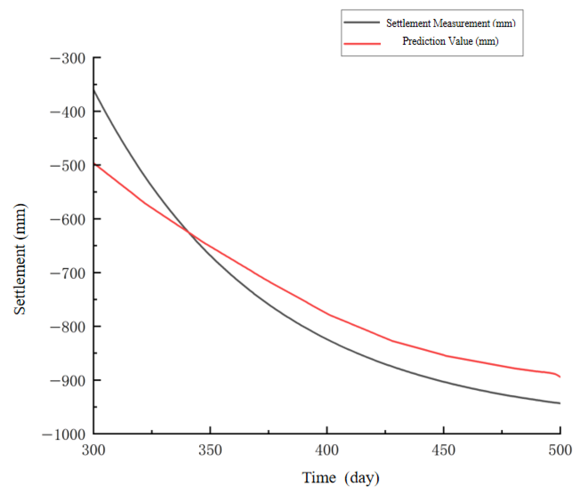
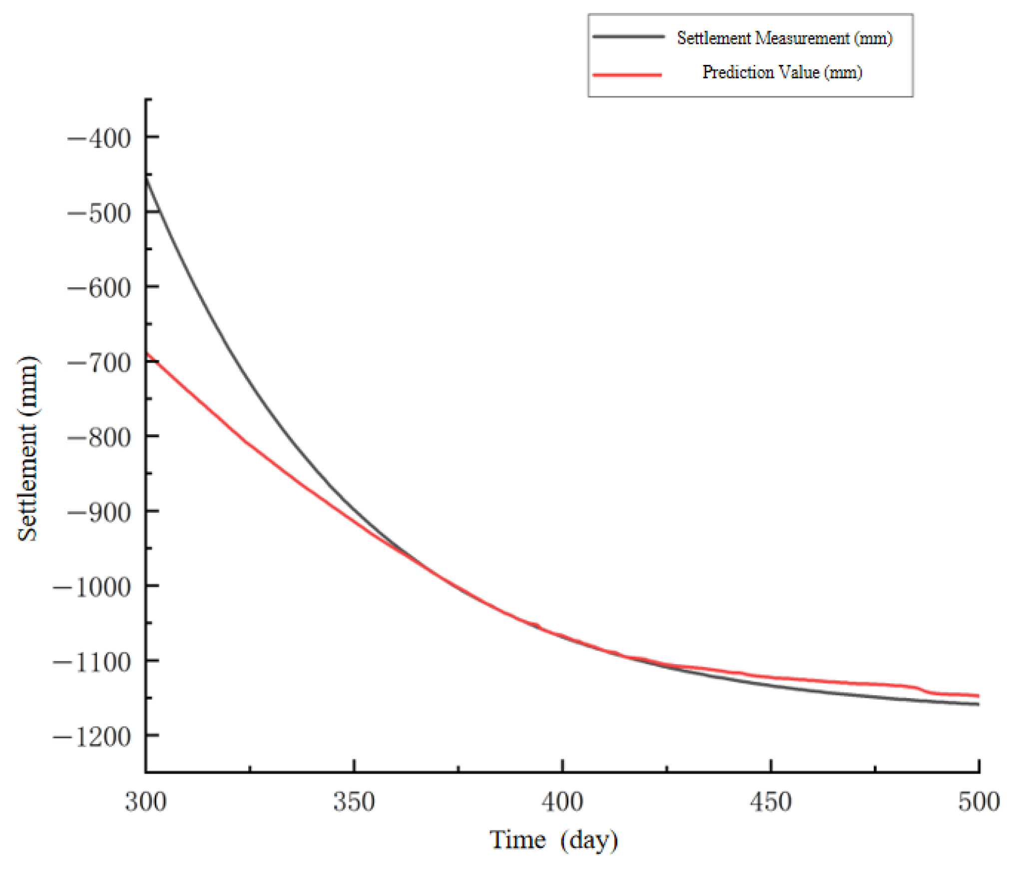
Using the values from the table above, we calculated the final settlement and relevant parameters (

Table 7. Calculation results of three-point method for each measuring point.

Measuring Point	$\mathit{\alpha }$	$\mathit{\beta }$	Predicting Settlement (mm)	Secondary Consolidation Settlement (mm)	${\mathit{S}}_{\mathbf{\infty }}$(mm)
CJ5	37.53	0.0136	−930.3	54.4	−984.7
CJ13	5.67	0.0071	−1197.0	55.3	−1252.3
CJ17	194.64	0.0192	−1158.9	70.5	−1239.4

). Figure 11, Figure 12 and Figure 13 subsequently compare the measured and predicted curves for the three observation points.

4.2. Hyperbola Method

The hyperbolic method assumes that the settlement value and time curve of the soil are hyperbolic after full-load preloading. The settlement time curve is fitted by the hyperbolic curve, and the curve equation is as follows [40]:

$$S=S_0+{\displaystyle \frac{\left(t-t_0\right)}{\alpha +\beta \left(t-t_0\right)}}$$

(21)

$S$—The settlement at time T;

$t_0$—Initial time;

$S_0$—Initial settlement amount;

$\alpha ,\beta$—Coefficient to be determined.

By transforming the above equation, we obtain

$${\displaystyle \frac{\left(t-t_0\right)}{\left(S-S_0\right)}}=\alpha +\beta \left(t-t_0\right)$$

(22)

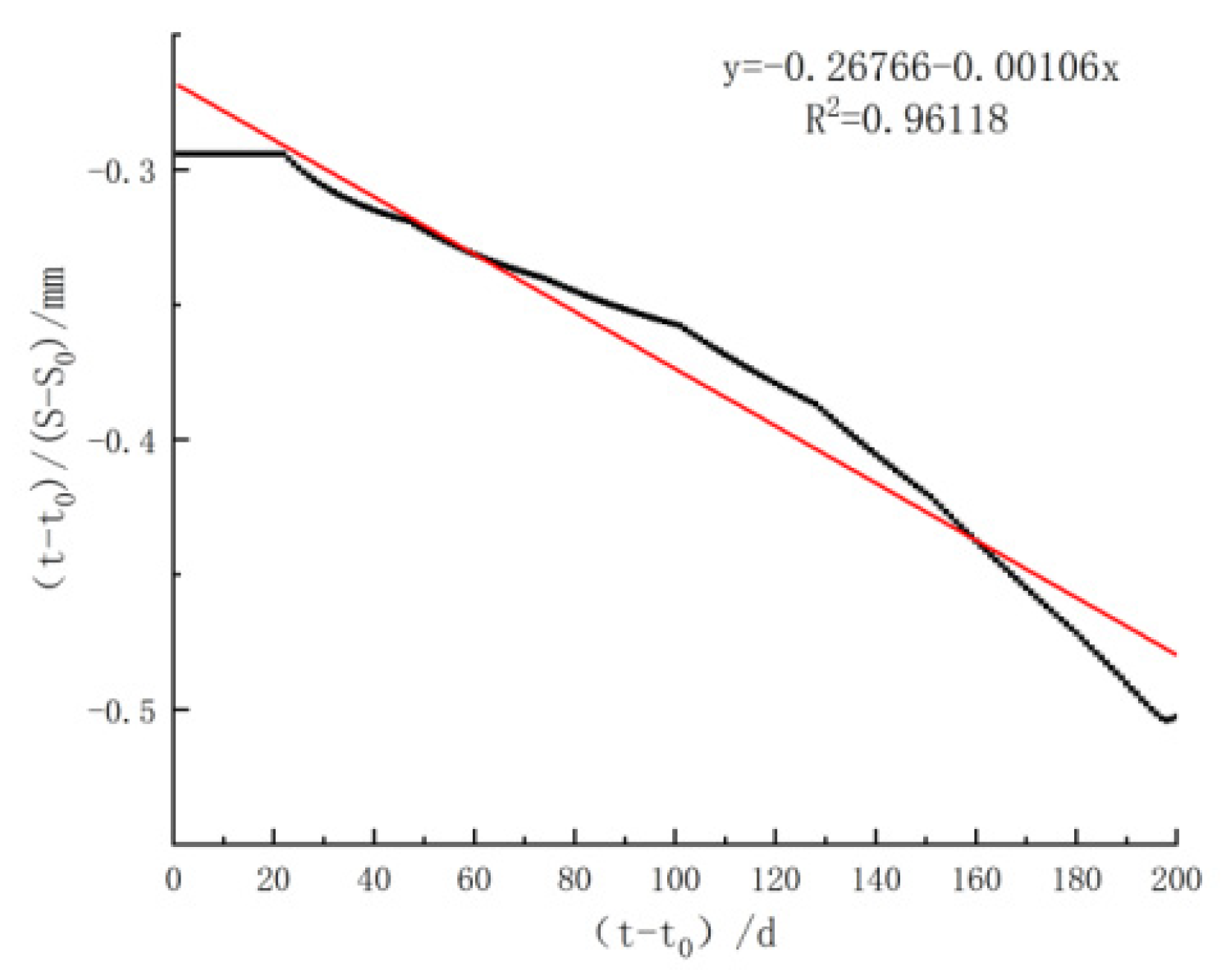
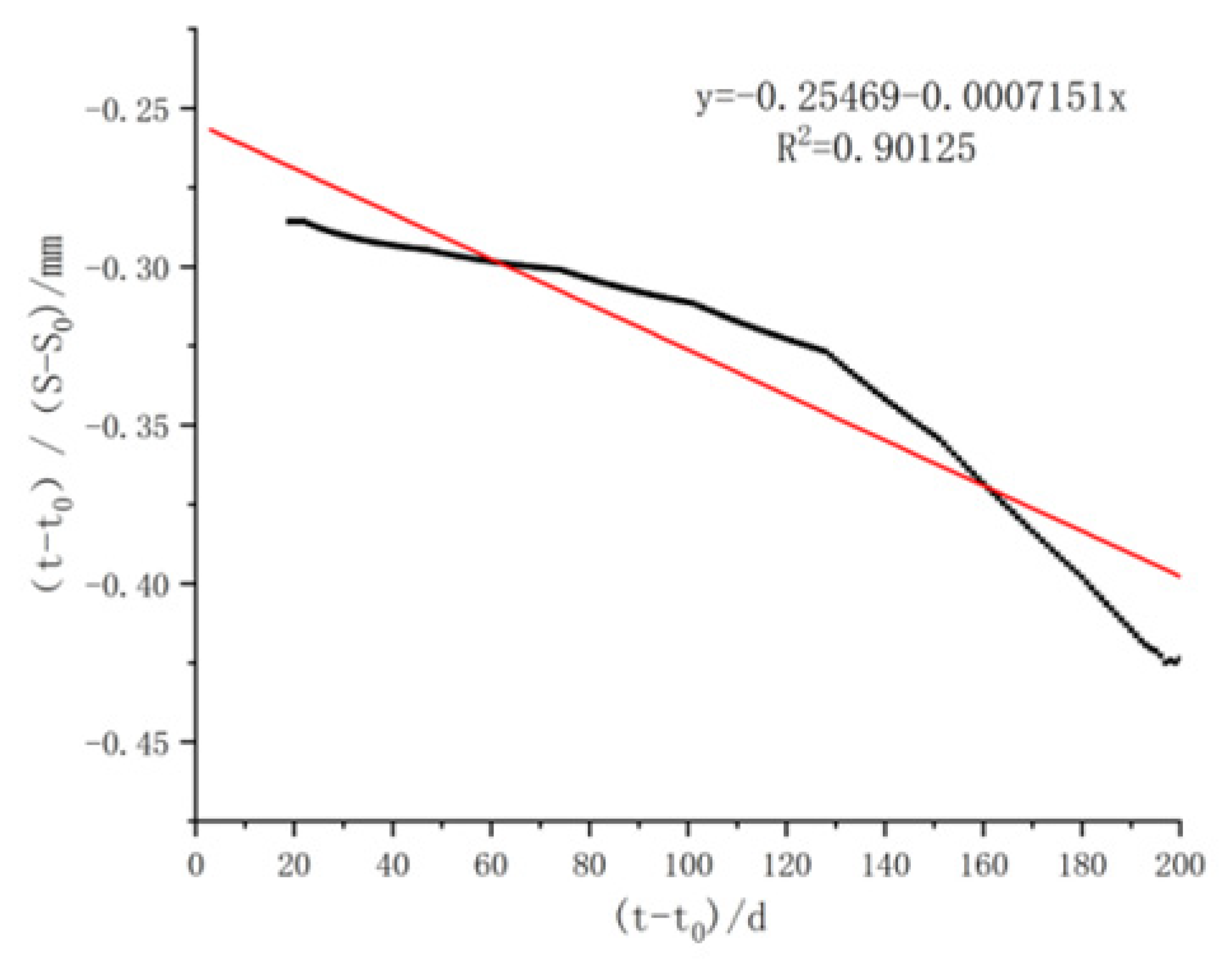
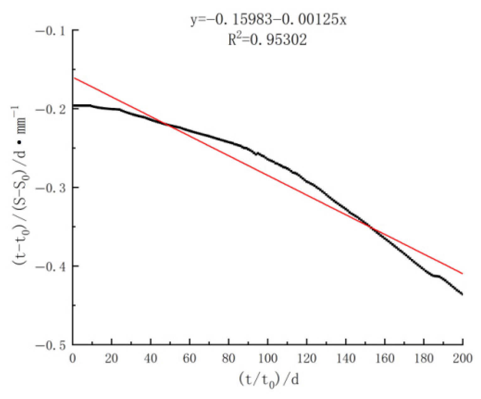
By using Origin software 7.0 to fit curves with coordinates ${\displaystyle \frac{\left(t-t_0\right)}{\left(S-S_0\right)}}$ and $\left(t-t_0\right)$, a straight line can be obtained. By substituting the undetermined coefficients $\alpha$, $\beta$, and $S_0$, obtained through fitting into Equation (21), the settlement S at any time point can be calculated. When t→$\infty$, the final settlement value can be inferred:

$$S_{\mathrm{\infty }}=S_0+{\displaystyle \frac{1}{\beta }}$$

(23)

The fitting parameters for the three measurement points (CJ5, CJ13, and CJ17) were determined separately and are presented in

Table 8. Calculation parameters of hyperbolic method for each measurement point.

Measurement Point	$\mathit{\alpha }$	$\mathit{\beta }$	R2
CJ5	−0.26766	−0.00106	0.96118
CJ13	−0.25469	−0.00071	0.90125
CJ17	−0.15983	−0.00125	0.95302

. The corresponding curve-fitting results are shown in Figure 14, Figure 15 and Figure 16.

By fitting the undetermined parameters obtained and substituting them into Equation (21), the settlement value at any time can be calculated using the formula. Figure 17, Figure 18 and Figure 19 show the comparison between the measured settlement curves of CJ5, CJ13, and CJ17 and the corresponding predicted settlement curves.

4.3. Comparison of Calculation Results

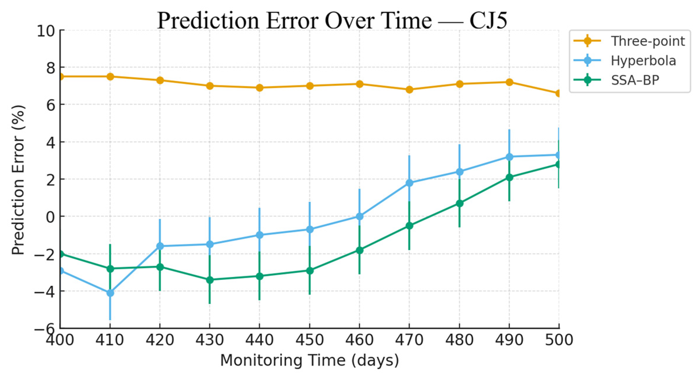
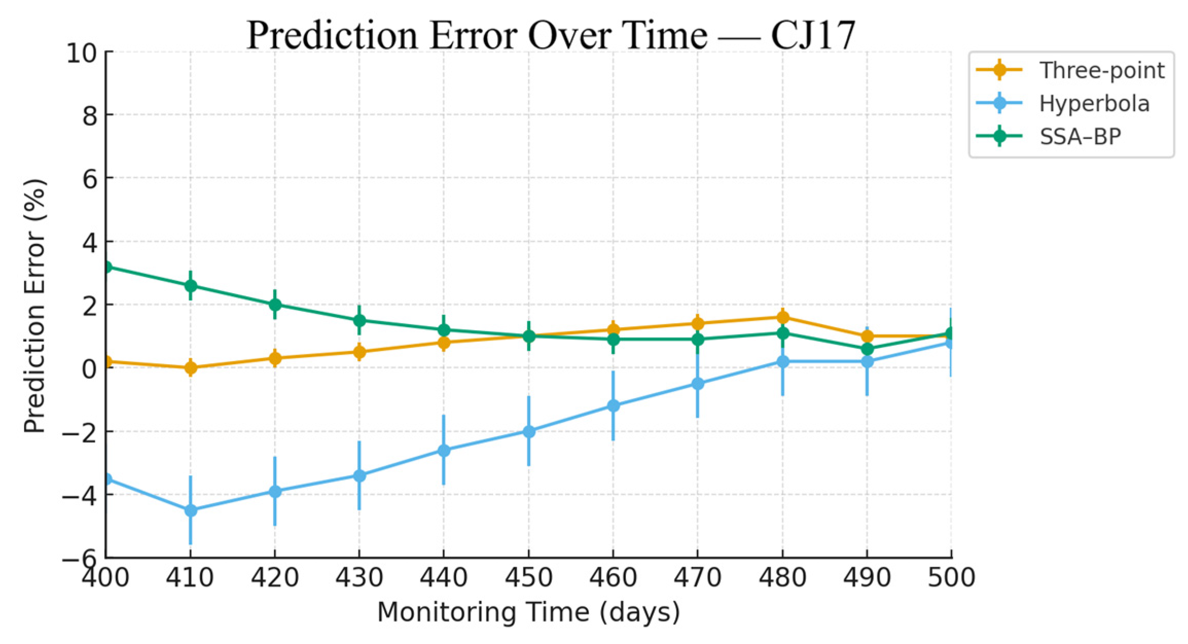
The three-point method, hyperbolic method, and SSA-BP neural network method were used to calculate and predict the settlement values of three measuring points, CJ5, CJ13, and CJ17, and compared them with the measured settlement data of the Xidong Road project to comprehensively evaluate the accuracy and applicability of each prediction method. All settlement monitoring data were obtained from in situ measurements and underwent manual verification for continuity and accuracy. Occasional missing records caused by instrument downtime were linearly interpolated. No smoothing or filtering was applied to preserve the original temporal variation in the data, and outliers were screened using the 3σ criterion prior to model training.

Table 9. Comparison between measured and predicted values of CJ5.

Monitor Time	Actuality (mm)	Three-Point Method		Hyperbola Method		SSA-BP
		Estimate (mm)	Error	Estimate (mm)	Error	Estimate (mm)	Error
400	−776.2	−834.1	7.5%	−753.9	−2.9%	−760.5	−2.0%
410	−794.8	−854.5	7.5%	−762.6	−4.1%	−772.5	−2.8%
420	−812.8	−872.3	7.3%	−800.2	−1.6%	−790.5	−2.7%
430	−829.6	−887.8	7.0%	−816.9	−1.5%	−801.2	−3.4%
440	−841.6	−899.3	6.9%	−832.8	−1.0%	−814.5	−3.2%
450	−853.6	−913.2	7.0%	−847.9	−0.7%	−828.8	−2.9%
460	−862.5	−923.5	7.1%	−862.2	0.0%	−847.2	−1.8%
470	−870.0	−929.5	6.8%	−885.9	1.8%	−865.6	−0.5%
480	−878.0	−940.4	7.1%	−898.9	2.4%	−884.0	0.7%
490	−883.4	−947.3	7.2%	−911.4	3.2%	−902.3	2.1%
500	−894.2	−953.3	6.6%	−923.3	3.3%	−919.2	2.8%

,

Table 10. Comparison between measured and predicted values of CJ13.

Monitor Time	Actuality (mm)	Three-Point Method		Hyperbola Method		SSA-BP
		Estimate (mm)	Error	Estimate (mm)	Error	Estimate (mm)	Error
400	−812.2	−837.4	3.1%	−777.9	−4.2%	−807.1	−0.6%
410	−837.6	−865.9	3.4%	−801.4	−4.3%	−832.8	−0.6%
420	−862.6	−892.4	3.5%	−824.0	−4.5%	−849.2	−1.6%
430	−885.6	−917.0	3.5%	−845.6	−4.5%	−862.5	−2.6%
440	−900.6	−940.0	4.4%	−866.3	−3.8%	−879.5	−2.3%
450	−915.6	−961.4	5.0%	−886.2	−3.2%	−885.6	−3.3%
460	−925.3	−981.4	6.1%	−905.3	−2.2%	−894.7	−3.3%
470	−934.2	−999.9	7.0%	−923.8	−1.1%	−908.5	−2.8%
480	−943.2	−1017.2	7.8%	−941.5	−0.2%	−919.6	−2.5%
490	−949.2	−1034.9	9.0%	−958.6	1.0%	−931.6	−1.9%
500	−962.9	−1048.3	8.9%	−975.1	1.3%	−951.3	−1.2%

and

Table 11. Comparison between measured and predicted values of CJ17.

Monitor Time	Actuality (mm)	Three-Point Method		Hyperbola Method		SSA-BP
		Estimate (mm)	Error	Estimate (mm)	Error	Estimate (mm)	Error
400	−1066.8	−1068.6	0.2%	−1029.5	−3.5%	−1100.5	3.2%
410	−1087.1	−1087.1	0.0%	−1038.4	−4.5%	−1115.2	2.6%
420	−1098.5	−1102.3	0.3%	−1055.7	−3.9%	−1120.5	2.0%
430	−1108.9	−1114.9	0.5%	−1071.7	−3.4%	−1125.4	1.5%
440	−1115.9	−1125.3	0.8%	−1086.5	−2.6%	−1129.5	1.2%
450	−1122.8	−1133.8	1.0%	−1100.3	−2.0%	−1133.9	1.0%
460	−1126.8	−1140.2	1.2%	−1113.1	−1.2%	−1137.1	0.9%
470	−1130.8	−1146.2	1.4%	−1125.0	−0.5%	−1141.2	0.9%
480	−1133.6	−1151.5	1.6%	−1136.1	0.2%	−1146.6	1.1%
490	−1144.5	−1155.5	1.0%	−1146.6	0.2%	−1151.2	0.6%
500	−1147.3	−1158.8	1.0%	−1156.4	0.8%	−1159.6	1.1%

show the final settlement results obtained by the above prediction methods. Figure 20, Figure 21 and Figure 22 provide the prediction error comparisons of CJ5, CJ13, and CJ17 using the three-point method, hyperbolic method, and SSA-BP neural network method.

The prediction results obtained by the traditional three-point method at the CJ17 monitoring point are relatively accurate; however, significant errors are observed at other locations. For instance, at CJ5, the prediction error reaches 7.5–7.7%, revealing the inherent limitations of this method, which relies on simplified assumptions and fails to capture the complex, site-specific behavior of the soil.

The hyperbolic method, which considers the variation law of the settlement curve during the preloading process, performs better than the three-point method. Nevertheless, its prediction error remains relatively high, with deviations of up to 4.5% at some monitoring points, indicating that the method still struggles to provide reliable long-term settlement predictions.

In contrast, the SSA-BP model demonstrates a markedly superior predictive performance and achieves consistently higher accuracy across all monitoring points. For example, at CJ5, CJ13, and CJ17, the prediction error of the SSA-BP model remains within a narrow range of −3.4% to 3.2%, confirming its outstanding stability and reliability. This superiority arises from the synergistic integration of the global optimization capability of the Sparrow Search Algorithm (SSA) and the nonlinear fitting strength of the BP neural network, which together enable the model to more accurately characterize the complex behavior of soft soil and effectively mitigate the local prediction errors that often occur in traditional approaches.

In summary, the SSA-BP model exhibits significant advantages in predicting soft foundation settlement. Compared with conventional empirical methods, it adapts more effectively to the nonlinear and heterogeneous characteristics of soil and delivers more accurate and stable prediction results, thereby providing strong theoretical support and technical assurance for real-time monitoring and dynamic regulation in practical soft foundation engineering.

5. Conclusions

This study proposes an intelligent prediction model (SSA-BP) to solve the problem of settlement prediction in soft soil foundations. The model combines the Sparrow Search Algorithm (SSA) with the BP neural network. Its core advantage is using SSA’s powerful global search capabilities. This allows for automatic optimization of the initial weights and thresholds of the BP network. As a result, it effectively overcomes limitations of the traditional BP model, such as sensitivity to local minima and insufficient prediction stability.

The study conducts comparative experiments with other optimization algorithms. These include Particle Swarm Optimization (PSO), Grey Wolf Optimization (GWO), and Differential Evolution (DE). Results indicate that the SSA-BP model has good convergence accuracy and robustness. The model is also verified using actual engineering monitoring data. Verification shows that the model’s prediction error across all measurement points is less than 4%. This demonstrates its ability to accurately capture the settlement characteristics of soft soils under surcharge preloading.

The study’s innovation lies in analyzing the nonlinear deformation behavior of the settlement process from an asymmetric perspective. The spatiotemporal evolution of soft soil settlement is significantly asymmetrical due to factors like heterogeneous soil composition, boundary constraints, and complex loading history. The SSA-BP model shows strong fitting and prediction ability for these asymmetric evolution patterns. It offers a new computational method to understand the complex deformation mechanisms of geotechnical systems. Compared with traditional empirical methods (such as the three-point and hyperbolic methods), the SSA-BP model has obvious advantages in handling the nonlinear and asymmetric nature of soft soil settlement.

The SSA-BP model has both theoretical and practical significance. It provides real-time and reliable decision support for unloading operations in dynamic design and construction. This improves risk control and cost efficiency. The study also highlights the potential of intelligent algorithms to reveal implicit mechanisms governing geotechnical system evolution, including both symmetric and asymmetric behaviors. Additionally, the model enhances project cost efficiency by reducing unnecessary resource allocation and avoiding expensive design changes.

However, some limitations should be noted. The SSA-BP model was developed and verified using data from a single construction project. This may limit the generalizability of the conclusions to other regions or geotechnical backgrounds. The dataset contains around 200 records over a limited observation period, mainly reflecting short-term consolidation behavior. This may not fully capture long-term settlement evolution, secondary compression effects, or soil–structure interactions under varying loading histories.

Moreover, the framework focuses on short-term rolling predictions. Its applicability to more complex boundary conditions requires systematic verification. Future research will focus on multi-site validation across diverse geological environments. It will also expand the framework using transfer learning or domain adaptation techniques. These efforts aim to promote broader applicability, enhance interpretability, and strengthen the role of intelligent algorithms in geotechnical engineering.

References

1. Li, Y.; Wu, H. The Application of Plastic Drainage Board Preloading Method in Hydraulic Embankments. Henan Water Conserv. South-North Water Divers. Proj. 2018, 47, 44–45. [Google Scholar]
2. She, Q. Application of Surcharge Preload Method in Soft Soil Foundation Treatment of Workshop. Fujian Archit. Constr. 2019, 1, 33–35. [Google Scholar]
3. He, P. The Study of Adopting PVD (Plastic Vertical Drain) Preloading Method in Sir Lanka South Railway Subgrade Construction. Constr. Des. For Eng. 2018, 70–73. [Google Scholar] [CrossRef]
4. Li, D.; Chen, L.; Chen, Y.; Hu, S.; Chai, Z. Application of artificial solidified crust—PVDs method in ground improvement: A case study. Transp. Geotech. 2023, 39, 100941. [Google Scholar] [CrossRef]
5. Yang, S.; Yang, A.; XUF. Vacuum preloading reinforcement of soft dredger soil by modified fiber drainage plate. Rock Soil Mech. 2025, 46, 789–797. [Google Scholar]
6. Zhang, C. The Application of Vacuum Combined with Preloading in the Treatment of Municipal Roads on Deep Soft Foundations. Sci. Technol. Innov. 2025, 193–196. [Google Scholar]
7. Shao, Z. Plastic Drainage Plate + Preloading Technology in Municipal Road Engineering. North. Build. 2024, 9, 26–29. [Google Scholar]
8. Chen, Y.; Chen, Y.; Chen, Z.; Lin, J.; Zhang, M. Research on Innovative Design of Combined Vacuum and Load Preloading Treatment Technology of Composite Plastic Drain Plate. Adhesion 2023, 50, 173–176. [Google Scholar]
9. Liu, X. Swirl Enhanced Drainage and Traditional PVC Drain in My Opinion. Sci. Technol. Inf. 2014, 222–223. [Google Scholar]
10. Cheng, Z. Study on the Settlement Prediction of Saturated Soft Clay by Plastic Drainage Board Preloading. Master’s Thesis, Zhejiang Sci-Tech University, Hangzhou, China, 2018. [Google Scholar]
11. Du, H.; Liu, J.; Yuan, Y.; Zhang, Y.; Song, S.; Xiao, H.; Huang, X. Study on The Methods of Ground Improvement for Widening Expressway on Soft Ground. In Proceedings of the 5th International Conference on Civil Engineering and Transportation 2015, Guangzhou, China, 28–29 November 2015; Atlantis Press: Paris, France, 2016; pp. 840–845. [Google Scholar]
12. Pan, Z. Research on the Application of Vacuum Preloading Technology in Soft Soil Foundation. Brick Tile 2025, 152–154. [Google Scholar]
13. Hu, X. Application and Discussion of Direct Drainage Method with Plastic Drainage Board Vacuum Preloading Construction Technology. West-China Explor. Eng. 2024, 36, 35–39. [Google Scholar]
14. Li, C.; Dias, D. Intelligent prediction and visual optimization of surface settlement induced by earth pressure balance shield tunneling. Tunn. Undergr. Space Technol. 2024, 154, 106138. [Google Scholar] [CrossRef]
15. Liao, M.; Wang, K.; Zhou, X.; Tian, L.; Wang, J.; Zhang, H.; Du, Y.; Yang, E. Development of an Intelligent Monitoring System for Settlement Prediction of High-Fill Subgrade. Infrastructures 2025, 10, 220. [Google Scholar] [CrossRef]
16. Hu, M.; Zhao, P.; Lu, J.; Wu, B. Mechanism-Driven Intelligent Settlement Prediction for Shield Tunneling Through Areas Without Ground Monitoring. Smart Cities 2025, 8, 6. [Google Scholar] [CrossRef]
17. Kovačević, M.; Hadzima-Nyarko, M.; Petronijević, P.; Vasiljević, T.; Radomirović, M. Comparative Analysis of Machine Learning Models for Predicting Interfacial Bond Strength of Fiber-Reinforced Polymer-Concrete. Computation 2025, 13, 17. [Google Scholar] [CrossRef]
18. Raju, M.; Shanmugam, K.P.; Shyu, C.R. Application of Machine Learning Predictive Models for Early Detection of Glaucoma Using Real World Data. Appl. Sci. 2023, 13, 2445. [Google Scholar] [CrossRef]
19. Gao, Y.; Zhang, Q.; Xu, Z. Optimization of Bridge Crane Main Beam Dimensions Based on Sparrow Search Algorithm and Finite Element Analysis. Highlights Sci. Eng. Technol. 2023, 79, 30–38. [Google Scholar] [CrossRef]
20. Xue, J.; Shen, B. A Survey on Sparrow Search Algorithms and Their Applications. Int. J. Syst. Sci. 2024, 55, 814–832. [Google Scholar] [CrossRef]
21. Zhang, H.; Zhang, Y. An Improved Sparrow Search Algorithm for Optimizing Support Vector Machines. IEEE Access 2023, 11, 8199–8206. [Google Scholar] [CrossRef]
22. Wang, T.; Zhou, H.; Liu, H. Multi-Label Feature Selection Based on HSIC and Sparrow Search Algorithm. Math. Biosci. Eng. 2023, 20, 14201–14221. [Google Scholar] [CrossRef]
23. Shi, G.; Li, R.; Li, F.; Niu, Y.; Yang, L. Depth Sensing with Coding-Free Pattern Based on Topological Constraint. J. Vis. Commun. Image Represent. 2018, 55, 229–242. [Google Scholar] [CrossRef]
24. Zhang, Y.; Liu, T.; Yang, F.; Yang, Q. A Study of Adaptive Fractional-Order Total Variational Medical Image Denoising. Fractal Fract. 2022, 6, 508. [Google Scholar] [CrossRef]
25. Liu, Q.; Zhang, Y.; Li, M.; Zhang, Z.; Cao, N.; Shang, J. Multi-UAV Path Planning Based on Fusion of Sparrow Search Algorithm and Improved Bioinspired Neural Network. IEEE Access 2021, 9, 124670–124681. [Google Scholar] [CrossRef]
26. Khaleel, M.I. Efficient Job Scheduling Paradigm Based on Hybrid Sparrow Search Algorithm and Differential Evolution Optimization for Heterogeneous Cloud Computing Platforms. Internet Things 2023, 22, 100697. [Google Scholar] [CrossRef]
27. Abdulhammed, O.Y. Load Balancing Of Iot Tasks in The Cloud Computing by Using Sparrow Search Algorithm. J. Supercomput. 2022, 78, 3266–3287. [Google Scholar] [CrossRef]
28. Jia, H.; Zheng, H.; Huo, S.; Zhou, H.; Zhang, Q. Autonomous Prediction of UAV Launch Parameters Based on SSA-BP Model. In Proceedings of the 2024 WRC Symposium on Advanced Robotics and Automation (WRC SARA), Beijing, China, 23 August 2024. [Google Scholar] [CrossRef]
29. Zhang, B.; Tao, X.; Zhang, H.; Yu, J. Study of an SSA-BP Neural Network-Based Strength Prediction Model for Slag–Cement-Stabilized Soil. Materials 2025, 18, 3520. [Google Scholar] [CrossRef]
30. Luo, J.; Wang, L.; Xiao, B.; Gao, S.; Li, W.; Deng, J.; Liang, C.; Xia, Y. Bending Prediction Of Bulb Flat Steel By Neural Network Algorithm Based On SSA-BP. In Proceedings of the 2024 IEEE International Conference on Cognitive Computing and Complex Data (ICCD), Qinzhou, China, 28–30 September 2024. [Google Scholar]
31. Lee, J.; Kim, K.; Kang, M.; Hong, E.S.; Choi, S. Void Detection for Tunnel Lining Backfill Using Impact-Echo Method Based on Continuous Wavelet Transform and Convolutional Neural Network. Geomech. Eng. 2024, 36, 1–8. [Google Scholar]
32. Yan, S.; Liu, W.; Li, X.; Yang, P.; Wu, F.; Yan, Z. Comparative Study and Improvement Analysis of Sparrow Search Algorithm. Wirel. Commun. Mob. Comput. 2022, 2022, 4882521. [Google Scholar] [CrossRef]
33. Karakaya, A.-S.; Köhler, K.; Heinovski, J.; Dressler, F.; Bermbach, D. A Realistic Cyclist Model for SUMO Based on the SimRa Dataset. In Proceedings of the 2022 20th Mediterranean Communication and Computer Networking Conference (MedComNet), Pafos, Cyprus, 1–3 June 2022; IEEE Conference Publication: Piscataway, NJ, USA, 2022. [Google Scholar]
34. Lawley, C.J.; Gadd, M.G.; Parsa, M.; Lederer, G.W.; Graham, G.E.; Ford, A. Applications of Natural Language Processing to Geoscience Text Data and Prospectivity Modeling. Nat. Resour. Res. 2023, 32, 1503–1527. [Google Scholar] [CrossRef]
35. Cang, N.; Qiu, F.; Xue, S.; Jia, Z.; Guo, D.; Zhang, Z.; Li, W. New Discrete-Time Zeroing Neural Network For Solving Time-Dependent Linear Equation with Boundary Constraint. Artif. Intell. Rev. 2024, 57, 140. [Google Scholar]
36. Tang, Y.; Xiao, S.; Zhan, Y. Predicting Settlement Along Railway Due to Excavation Using Empirical Method and Neural Networks. Soils Found. 2019, 59, 1037–1051. [Google Scholar] [CrossRef]
37. Chung, S.G.; Kweon, H.J. Prediction of Three-Dimensional Consolidation Settlement: Observational Method and Its Applicability. Int. J. Geomech. 2023, 23, 04022308. [Google Scholar] [CrossRef]
38. Wang, Z.; Xie, X.; Wang, J. A New Nonlinear Method for Vertical Settlement Prediction of A Single Pile and Pile Groups in Layered Soils. Comput. Geotech. 2012, 45, 118–126. [Google Scholar] [CrossRef]
39. Huang, G. Problems and Their Solutions in Predicting Soft Ground Settlement Based on Asaoka’s Method. Rock Soil Mech. 2016, 37, 1061–1065. [Google Scholar]
40. Wu, Y. Research on Settlement Monitoring and Prediction of Soft Soil Roadbeds on Highways. Jiangxi Jiancai 2024, 301–303. [Google Scholar]
Figure 1. Geographical location map of Xidong Road project.
Symmetry 17 01989 g001
Figure 2. Schematic diagram of preloading method for plastic drainage board stacking.
Symmetry 17 01989 g002
Figure 3. SSA-BP model construction process diagram.
Symmetry 17 01989 g003
Figure 4. Test function image.
Symmetry 17 01989 g004
Figure 5. Settlement over time.
Symmetry 17 01989 g005
Figure 6. Evolutionary curves of SSA and GA.
Symmetry 17 01989 g006
Figure 7. Comparison of settlement value prediction curves.
Symmetry 17 01989 g007
Figure 8. Comparison of prediction errors for settlement values.
Symmetry 17 01989 g008
Figure 9. Comparison chart of prediction error percentage of settlement value.
Symmetry 17 01989 g009
Figure 10. Flowchart of curve fitting method.
Symmetry 17 01989 g010
Figure 11. Comparison between predicted settlement and measured settlement using CJ5 three-point method.
Symmetry 17 01989 g011
Figure 12. Comparison between predicted settlement and measured settlement using CJ13 three-point method.
Symmetry 17 01989 g012
Figure 13. Comparison between predicted settlement and measured settlement using CJ17 three-point method.
Symmetry 17 01989 g013
Figure 14. CJ5 curve fitting diagram.
Symmetry 17 01989 g014
Figure 15. CJ13 curve fitting diagram.
Symmetry 17 01989 g015
Figure 16. CJ17 curve fitting diagram.
Symmetry 17 01989 g016
Figure 17. CJ5 hyperbolic method prediction curve.
Symmetry 17 01989 g017
Figure 18. CJ13 hyperbolic method prediction curve.
Symmetry 17 01989 g018
Figure 19. CJ17 hyperbolic method prediction curve.
Symmetry 17 01989 g019
Figure 20. Comparison of CJ5 prediction errors. Statistical analysis was conducted using one-way ANOVA (p < 0.05).
Symmetry 17 01989 g020
Figure 21. Comparison of CJ13 prediction errors. Statistical analysis was conducted using one-way ANOVA (p < 0.05).
Symmetry 17 01989 g021
Figure 22. Comparison of CJ17 prediction errors. Statistical analysis was conducted using one-way ANOVA (p < 0.05).
Symmetry 17 01989 g022