Article

Design of Network Anomaly Detection Model Based on Graph Representation Learning

Department of Computer Science, Guangdong University of Science and Technology, Dongguan 523668, China
*
Author to whom correspondence should be addressed.
Symmetry 2025, 17(11), 1976; https://doi.org/10.3390/sym17111976
Submission received: 15 September 2025 / Revised: 24 October 2025 / Accepted: 12 November 2025 / Published: 15 November 2025
(This article belongs to the Special Issue Applications Based on Symmetry in Adversarial Machine Learning)

Abstract

Network attacks are becoming increasingly diverse and sophisticated, resulting in complex cybersecurity challenges, which can be fundamentally viewed as a disruption of the symmetry or balanced state in normal network behavior. To address these challenges, graph representation learning methods have gained prominence in network anomaly detection. These methods effectively represent complex network traffic data as graphs and capture data relationships. By integrating deep learning, graph neural networks, and other techniques, graph representation learning enhances the accuracy and efficiency of network anomaly detection in complex network environments. This paper proposes a novel network anomaly detection model based on graph representation learning called ETG-EESAGE. The model constructs an event key time subgraph (ETG) to group similar data and enhance structural features. Then, it introduces an edge enhancement sampling aggregation algorithm (EESAGE) to capture node relations and differentiate edge information accurately. The model generates richer node feature representations during aggregation and detects abnormal nodes using a threshold. Experimental evaluations on the CIC-IDS2017 dataset demonstrate the strong performance of the proposed model across multiple daily subsets. Under optimal configuration settings, ETG-EESAGE achieves an average accuracy of 95.5%, precision of 97.9%, recall of 97.3%, and F1-score of 97.7%, outperforming other baseline algorithms. The model also exhibits strong interpretability and applicability in real-world network anomaly detection scenarios.

1. Introduction

With the continuous improvement of network technology and the rapid expansion of network scale, cybersecurity issues have become increasingly prominent. Unlawful individuals exploit network vulnerabilities using progressively sophisticated techniques, rendering software, hardware, and users’ information more vulnerable to internal and external security threats.
Network anomaly detection plays a vital role in the field of cybersecurity by identifying significant and uncommon events in the network and triggering necessary actions in various application scenarios. From the perspective of symmetry, normal network operations often exhibit stable patterns and balanced structures—such as periodic traffic flows, consistent protocol behaviors, and harmonious interactions between entities—which can be viewed as a form of symmetry. Anomalies, conversely, represent a deviation or break in this symmetry, manifesting as irregular traffic, atypical communication patterns, or imbalances in system resource usage. Network anomaly detection involves identifying patterns in network traffic data that deviate from expected behavior, and the specific terminology used to describe these deviations varies across different application scenarios [1]. The definition proposed by Hawkins et al. [2] in 1980, which suggests that anomalies differ significantly from other observed results to the extent that they raise suspicion of being generated by different mechanisms, is widely accepted.
In reality, data is often interconnected and does not exist independently [3]. These interdependencies can be naturally represented using graph models. Additionally, network threats often exhibit correlations, where points that are close to anomalies are also likely to be anomalies [4,5]. Therefore, converting network traffic data into graph data for network anomaly detection is a viable approach [6]. As large-scale network data graphs become more prevalent, researchers have proposed improved methods for graph representation learning that can directly process data. Utilizing such learning methods for network anomaly detection allows for more precise exploration of relationships between data, representing the intricate and diverse data in a concise graph format. By analyzing and processing the graph data, complex multi-step attacks or associated threats can be discovered.
This paper proposes a novel network anomaly detection model called ETG-EESAGE (Event key Time subgraph and Edge Enhancement Sampling Aggregation). The model comprises four main components: data pre-processing, construction of event key time subgraphs (ETG), edge enhancement sampling aggregation algorithm (EESAGE), and anomaly detection. The network anomaly detection process starts by transforming, extracting, and selecting features from the raw network traffic data. Then, event key time subgraphs are constructed based on the preprocessed network traffic dataset. Next, the edge enhancement sampling aggregation algorithm is applied to generate new feature representations for each node in the subgraph. Finally, anomalies are detected by setting a detection threshold. The contributions of this paper can be summarized as follows:
  • Based on the identified characteristics of network anomalies, such as “device aggregation” and “activity aggregation” [7], and the main features generated by network traffic data, we propose a novel graph construction method that constructs event key time subgraphs on network traffic data. Unlike other graph construction methods, this method enables the aggregation of data with similar features and obtains a more compact, accurate, and comprehensive representation of data relationships and structural features. Moreover, this construction method reduces graph complexity and improves detection efficiency.
  • We propose an edge enhancement sampling aggregation algorithm for representation learning on the constructed event key time subgraphs. The algorithm consists of two parts: the edge selection sampling algorithm and the edge enhancement aggregation algorithm. The edge selection sampling algorithm captures accurate correlation relationships between nodes and differential information among different edges. In the aggregation phase, the edge enhancement aggregation can obtain more comprehensive node feature representations without the need for multiple layers of aggregation or complex aggregation functions.
The remainder of this article is organized as follows. Section 2 reviews related work on network anomaly detection, including traditional machine learning, deep learning, and graph-based methods. Section 3 introduces the proposed ETG-EESAGE model, detailing its architecture, graph construction, and optimization strategies. Section 4 describes the experimental setup, datasets, evaluation metrics, comparative algorithms, and presents and discusses the experimental results. Finally, Section 5 concludes the study and outlines potential directions for future work.

2. Related Work

With the rapid development of Internet plus and the explosive growth of data volume, the limitations of traditional detection methods have become increasingly prominent. The rule-based detection methods proposed by Ding et al. [8] and others, although simple and intuitive, rely on human experience for rule formulation, making it difficult to cope with complex and changing network environments; the statistical analysis-based detection methods proposed by Goldman et al. [9] and Ye et al. [10], although capable of capturing the distribution characteristics of data, are prone to false positives and false negatives, limiting their effectiveness; the machine learning-based detection methods proposed by Wang et al. [11] and Su et al. [12], although capable of automatically learning features, face high costs in model training and maintenance when dealing with large-scale, high-dimensional data, and have a strong dependence on feature engineering.
However, with the rise of deep learning-based detection methods, the malicious code detection method based on an autoencoder and DBN proposed by Li et al. [13] and the unsupervised anomaly detection method using GAN proposed by Schlegel et al. [14] have shown great potential in addressing the challenges related to detecting complex network attacks and threats. Liu et al. [15] proposed a visual transformation and spatio-temporal traffic classification method based on the attention mechanism. They used the transformer encoder and multi-head self-attention mechanism to capture the global features of session images. At the same time, they adopted convolution operations and the attention mechanism to extract spatio-temporal features through bidirectional long-short-term memory. Finally, they fused the global features and spatio-temporal features through a dynamic weighting mechanism to classify encrypted traffic. Graph representation learning methods are widely adopted for their ability to represent large and complex network traffic data in a concise graphical format and effectively explore the relationships between data points. The combination of deep learning and graph neural network technologies enables graph representation learning to better handle the complexity and diversity of network environments, improving the accuracy and efficiency of network anomaly detection.
For supervised graph representation learning methods, such as the log2vec heterogeneous graph embedding model proposed by Liu et al. [16] in the context of enterprise-level network threat detection, they usually treat log entries with five meta-attributes as graph nodes and establish connections between nodes. However, the unique construction and random walk rules of this model may introduce redundant logarithmic relationships, which may affect clustering results. Cai et al. [17] proposed an end-to-end structured temporal graph neural network model, strGNN, based on the characteristics of network traffic data that changes over time in reality and the potential addition or deletion of connection relationships between nodes due to the arrival of new data. However, this model often encounters difficulties in effectively processing large-scale data and capturing global graph properties and long-term dependencies. In summary, current supervised network anomaly detection models face challenges such as complex graph construction and high computational costs. Xiao et al. [18] decouple local proximity from global periodicity in their S2TAT module, guiding our timestamp-aware edge sampling, while Zhang et al. [19] achieve state-of-the-art anomaly discrimination with only a single-layer adversarially regularized aggregator, motivating our edge-enhanced aggregation that harvests rich features without deep stacking. ISC-QL [20] combines Improved Spectral Clustering and Q-Learning for edge server placement in Intelligent Transportation Systems, achieving significant improvements in load balancing, energy efficiency, and latency. This demonstrates strong practical applicability in IoV environments.
In summary, traditional rule-based and statistical methods are simple but rely heavily on expert knowledge and often suffer from high false alarm rates. Machine learning approaches can automatically learn features, but are costly to train and maintain when dealing with large-scale data. Deep learning methods enhance feature extraction yet require substantial data and resources. Recently, graph representation learning has shown great potential in modeling complex network relationships, though existing supervised models like Log2Vec and StrGNN still face issues such as redundant connections and high computational cost.
To address these challenges, this paper proposes the ETG-EESAGE (Event Timestamp Graph and Edge Enhancement Sampling Aggregation) model, which integrates event-timestamp-based subgraph construction and edge enhancement aggregation to achieve compact graph representation and efficient anomaly detection. This model is based on the characteristics of network anomalies discovered in the study, such as “device aggregation” and “activity aggregation”, as well as the main characteristics of network traffic data. It proposes a novel graph construction method that targets the characteristics of network anomalies and network traffic data, making it highly likely that data with the same characteristics are clustered together to obtain more compact, accurate, and comprehensive data relationships and structural features. Moreover, this graph construction method can reduce the complexity of graph construction and improve detection efficiency. In addition to better capturing the accurate correlation between nodes and the difference between different neighboring edges, and to obtain richer new node features without the need to add multiple layers of aggregation or complex aggregation functions, the neighboring edge selection sampling algorithm and the neighboring edge enhancement aggregation algorithm are adopted. The purpose is to reduce computational costs and reduce the complexity of graph construction while ensuring detection efficiency.

3. Proposed Framework

3.1. Overview

The main purpose of our ETG-EESAGE model is to detect network anomalies by transforming the network traffic data into a graph and learning the embedding vectors of the nodes in the graph, which are then used to determine whether the nodes are abnormal or not. As shown in Figure 1, the model consists of four main components:
  • Data Pre-processing: To address the issues of inconsistency and incompleteness in the original network data, our ETG-EESAGE model first performs data pre-processing, which includes data replacement, feature extraction, and selection. This process improves the quality of the data and enhances the efficiency of data analysis.
  • ETG Construction: Based on the characteristics of network traffic data and network anomalies such as “device aggregation” and “activity aggregation”, the data is divided into subsets based on timestamp characteristics, resulting in several data sets within the same timestamp and across different periods. With this approach, we define a network event as a graph node and the different relationships between the nodes as edges to construct the event key time subgraph (ETG).
  • EESAGE Algorithm: The Edge Enhancement Sampling Aggregation (EESAGE) algorithm has two main components: neighboring-edge selection sampling and neighboring-edge enhancement aggregation. In the neighboring-edge selection sampling algorithm, the neighboring nodes are first selected and sampled based on their correlation. In the neighboring-edge enhancement aggregation algorithm, the mean aggregation function is used to aggregate the node’s features, neighboring node features, and neighboring edge label features simultaneously. This process results in a more accurate and comprehensive node.
  • Detection Algorithm: By setting a detection threshold, the model can determine whether the network event represented by the node is abnormal or not. This method allows for intuitive understanding and interpretation of the detection results and is applicable to various types of data.
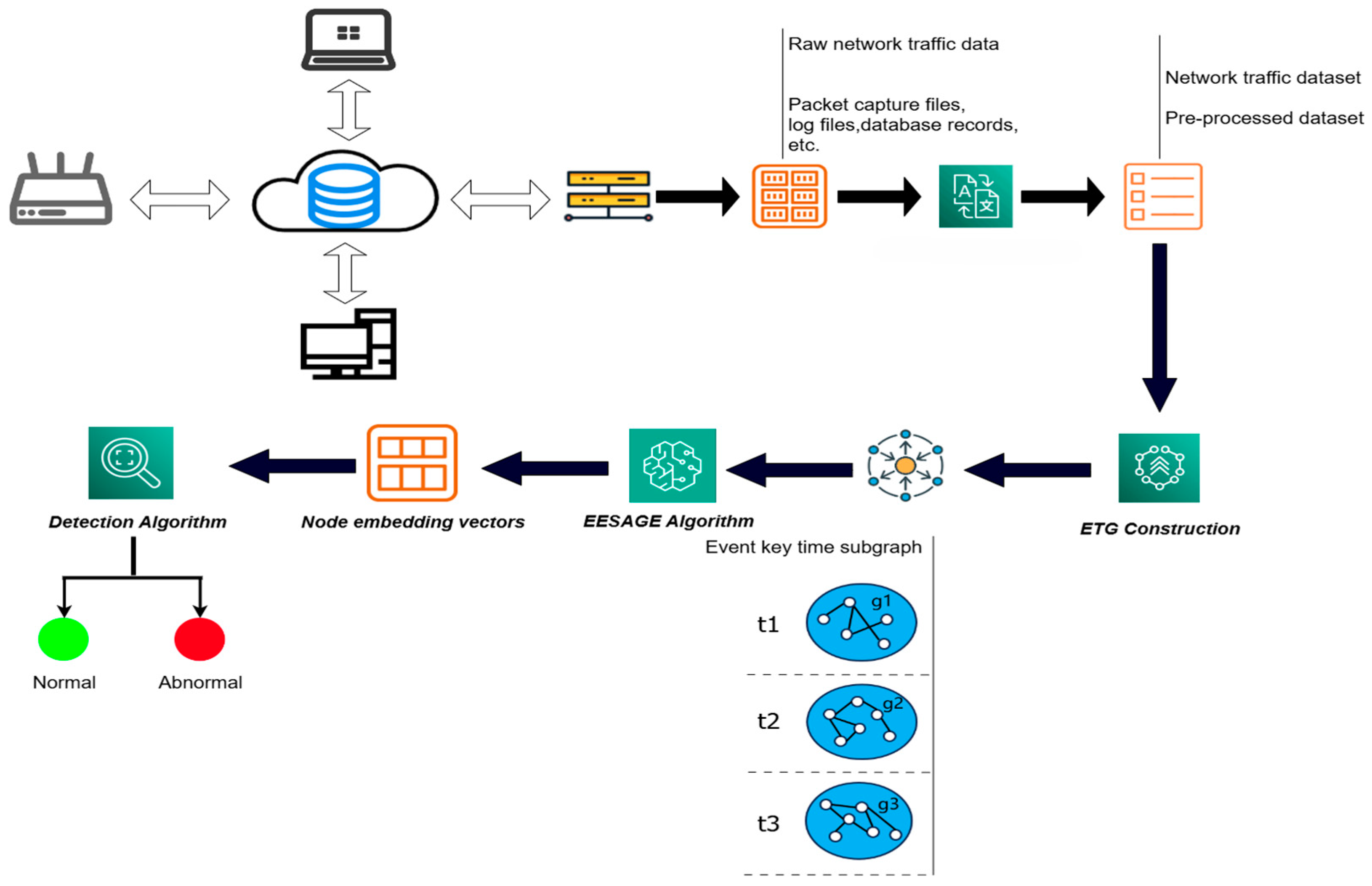
Figure 1. Overview of the ETG-EESAGE-based network anomaly detection model.
Symmetry 17 01976 g001

3.2. Data Pre-Processing

3.2.1. Workflow of Pre-Processing

As shown in Figure 2, the raw network traffic data generated by network devices or applications is first processed using a feature extraction tool to extract representative and distinguishing features. These features may include source IP address, destination IP address, source port, destination port, protocol, timestamp, flow duration, total forward packets, etc.
The feature-extracted network traffic dataset is then defined as D, and each data entry d undergoes a transformation process. This process involves replacing NaN values and normalizing the data using the MinMax Normalization. The Information Gain algorithm is then applied to select a set of feature categories that exhibit a strong relation with anomalous performance. Finally, the data are sorted in chronological order based on their generation timestamp, resulting in the new network traffic dataset D’.

3.2.2. Data Transformation

NaN (Not a Number) replacement: In the real world, network traffic data has the characteristics of incompleteness, vulnerability, and easy loss, which leads to the invalidation of specific values. And these missing or invalid values are usually represented by NaN. In this study, in order to maintain the integrity of the model and avoid data loss and changes in the relationships between nodes, a value of 0 was used for replacement in the presence of a small number of NaN values in the dataset.
Normalization: To restrict data values within a certain range and prevent small data from being overshadowed, this model employs the MinMax Normalization. This algorithm linearly transforms the input data to obtain a range between 0 and 1. The specific formula used for this normalization is as follows:
X n o m = x x m i n x m a x x m i n
where X represents the input data, x m a x and x m i n represent the maximum and minimum values in the data, respectively.
IP Address Transformation: Since IP addresses are categorical identifiers, each IPv4 address was decomposed into four decimal components corresponding to different hierarchical levels of the network. These components were then normalized to the [0, 1] range using normalization to eliminate scale differences while preserving subnet correlations. The four normalized components were subsequently used as independent input features to retain fine-grained network segment information relevant to fraud-device clustering detection.
Timestamp Transformation: All timestamps were first standardized to Unix time format (in seconds) and then converted into two kinds of numerical features. Relative time difference, computed as the elapsed time from the dataset’s start timestamp, preserving temporal order and intervals for event–time graph construction. Cyclic time features, optionally encoded by their occurrence probability in the dataset to capture periodic behavioral patterns. Both types of time features were normalized to the [0, 1] range before being fed into the model, ensuring numerical consistency across features.

3.2.3. Feature Selection

There are various types of features extracted from the raw data, each serving different purposes. For example, IP addresses and port numbers are used to identify the sender and receiver in a network communication. By analyzing these features, anomalies can be effectively detected with a high probability. On the other hand, certain features may exhibit a weak correlation to anomalous performance, meaning they are less informative in identifying anomalies.
In order to improve detection performance while minimizing storage and time costs, this model incorporates a technique proposed by Kurniabudi et al. [21]. The method employs an Information Gain algorithm to select features from the network traffic data that are strongly correlated with anomalous performance. These selected features are then utilized as attributes for graph nodes in subsequent representation learning. The Information Gain algorithm primarily calculates the entropy of each feature in the network traffic data, as demonstrated by the following formula:
E n t r o p y S = i c P i log 2 P i
where c represents the number of data categories and P i represents the number of samples with category i . After obtaining the entropy, the information gain value can be obtained by the following equation:
G a i n S , F = E n t r o p y S V a l u e F S x S E n t r o p y S x
where S represents the sample, F represents the feature, x represents the possible values of feature F , such as the possible values of protocols are HTTP, HTTPS, FTP, etc., V a l u e F represents all possible values of feature F , S x represents the number of samples containing x , | S | represents the number of samples of all data, and E n t r o p y S x represents the entropy of the samples containing x .
The information gain values obtained from these calculations are then sorted, and the features with the highest correlation to anomaly detection are selected as node features for representation learning.

3.3. ETG Construction

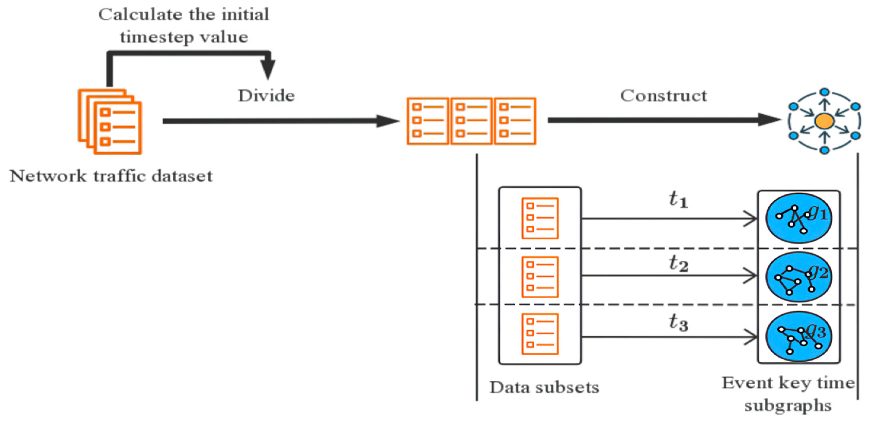
To construct event key time subgraphs based on the characteristics of network traffic data and network anomalies, this model follows a process that involves computing the initial timestamp value, dividing data subsets, and applying graph construction rules. To better comprehend the principles of graph construction, this chapter begins by introducing the motivation behind it. Subsequently, as illustrated in Figure 3, the process of constructing is described.

3.3.1. Construction Motivation

As network technology advances, network attacks have become increasingly complex and difficult to detect. However, certain limitations imposed by objective factors create specific patterns and characteristics in the generated network anomalies. Research has identified two notable characteristics of network anomalies: “device aggregation” and “activity aggregation”.
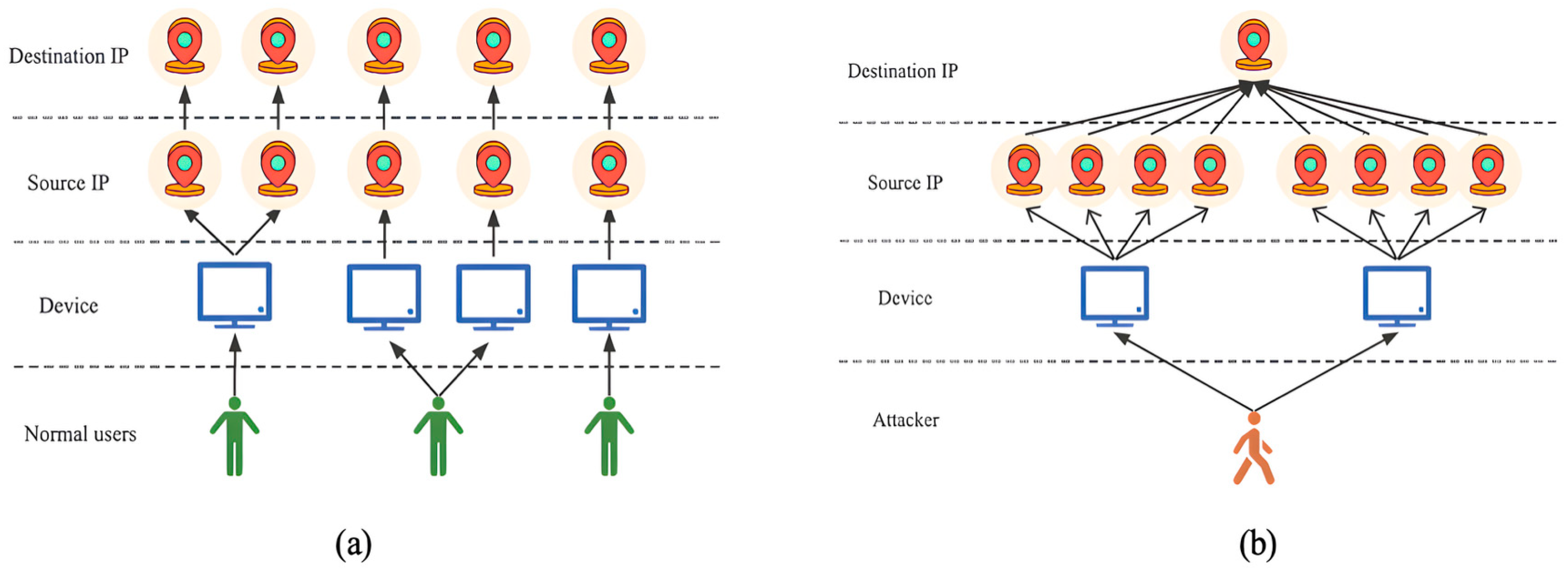
Device aggregation: Figure 4a illustrates that normal users typically utilize one or two devices for network communication, and their network activities are associated with a single IP address per device, assuming no virtual machines or proxy gateways are used. On the other hand, Figure 4b shows that attackers engaged in malicious activities often employ multiple IP addresses to launch frequent attacks on specific targets, aiming to obfuscate their identities. However, due to constraints in economic and computational resources, attackers often rely on virtualization or proxy techniques to obtain multiple IP addresses using a limited number of devices. This behavior demonstrates the “device aggregation” characteristic of attackers. Suspicion arises when a small number of devices exhibit frequent activities to specific targets using multiple different IP addresses, as this indicates potentially malicious behavior within the network.
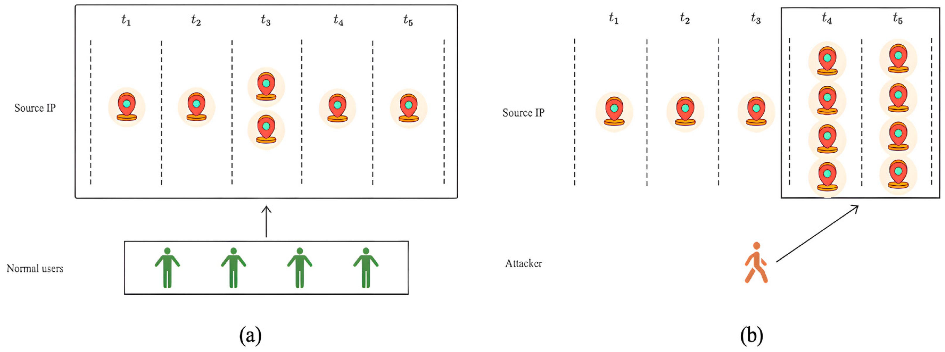
Activity aggregation: In Figure 5a, a normal network environment exhibits a certain pattern in the number of devices and IP addresses present during different periods. Although there may be fluctuations within a day, over a longer period of activity, the distribution of devices and IP addresses follows a specific pattern. In contrast, attackers face time constraints and must complete their attack tasks within specific time frames. This results in a concentrated surge of attack activities during a particular period, demonstrating the characteristic of “activity aggregation”. As depicted in Figure 5b, compared to the normal network environment, there is a higher concentration of IP addresses at t 4 and t 5 in this network environment. Based on the analysis, these IP addresses are considered suspicious.
Use a timestamp to capture network anomalies: Analyzing the network traffic data within the same time provides a clearer view of the “aggregation” characteristics of network anomalies. Furthermore, data generated at the same time tend to exhibit more similar characteristics compared to data generated at different times. To leverage this insight, the model adopts a two-step approach during the graph construction stage. Firstly, the network traffic dataset is divided into multiple subsets based on its timestamp feature. Subsequently, a subgraph is constructed for each subset. The subsequent subsections provide a detailed description of the specific construction process.

3.3.2. Calculate the Initial Timestamp Value

Before graph construction, it is necessary to calculate an initial timestamp value (timestamp), which is used to divide the network traffic dataset. D into several subsets within the same timestamp and between different time periods, and then construct an event key time subgraph for each data subset. The selection of the initial value is crucial, as it directly affects the graph construction and subsequent representation learning. If the value is too large, data with similar features may not be properly aggregated. Conversely, if the value is too small, the graph may not capture enough neighboring features. Moreover, excessively dividing the graphs will increase the storage cost of the detection model.
Therefore, based on observations of the data and the “aggregation” characteristics of network anomalies, as well as conducting computational experiments with a small number of data samples, we propose the following hypothesis: when network anomalies are concentrated in specific time periods, the amount of data within these time periods should be equal to the potential number of network anomalies.
Based on this assumption, this model utilizes three variables: the data volume ( D ), the time length ( t i m e l e n ), and the ratio of network anomaly data to the overall data volume ( r a t i o ) to calculate the timestamp. The r a t i o will vary depending on the network environment and data type. In certain network environments, network anomaly data may constitute a relatively large proportion, while in others, it may be relatively small. Therefore, the selection of a ratio needs to consider various factors such as network size, traffic, usage, and security threats. It should be chosen appropriately based on the specific circumstances.
Based on the above analysis, the timestamp can be calculated using the following formula,
t i m e s t e p = D × r a t i o / D t i m e l e n α = t i m e l e n × r a t i o α
where D t i m e l e n represents the data generated per unit time in D , and D × r a t i o represents the number of data points generated in D related to network anomalies in the current network environment. The hyperparameter α is used to determine the number of possible anomalous occurrences. The selection of α should be based on the data distribution and experimental analysis. The t i m e l e n × r a t i o represents the product of the time length and the proportion of anomalous data, which is used to calculate the time steps.
When the data in D are equally distributed per unit time, the ratio of network anomaly data to the total data volume is equivalent to the ratio of the time when the network anomaly occurs to the total time length. Therefore, the simplified formula is consistent with the initial assumption.
The calculated initial timestamp value serves as a starting point for dividing the dataset based on the assumptions. However, due to the complexity of real-world network traffic data, this value is considered an initial estimate and may need further adjustment based on data analysis and experimental results. The goal is to fine-tune the timestamp value to achieve the best detection performance for the model.

3.3.3. Divide Data Subsets

The network traffic dataset is divided based on the timestamp using Algorithm 1. After preprocessing, the dataset is denoted as D , and T represents the set of unique and non-repeating timestamp features in the dataset. The dataset start time is t 1 , and the end time is t n . The timestamp divides D into multiple data subsets D s = D 1 D 2 D m within the same timestamp and between different time periods. The value of m , obtained in step 2 by rounding up, indicates the number of time periods and the corresponding number of data subsets after division based on the timestamp.
Algorithm 1: Divide data subsets
Input:
pre-processed dataset D ;
timestamp set Τ = { t 1 , t 2 , , t n } ;
timelen;
timestamp;
Output: data subsets ( D s = D 1 D 2 D m )
1: m t i m e l e n t i m e s t a m p
2: i 1
3: for d D do
4:   if g e t T i m e s t a m p d < t 1 × t i m e s t e p then
5:        D i D i { d }
6:   else
7:        i i + 1
8:        D i D i d
9:   end if
10: end for
Specifically, the set of timestamp features T = t 1 , t 2 , , t n the dataset can be divided into subsets based on the timestamp as follows:
t 1 , t 1 + T i m e s t e p ,   t 1 + T i m e s t e p , t 1 + 2 × T i m e s t e p ,   ,   t 1 + m 1 × T i m e s t e p , t n ] ,
Each subset of timestamp features corresponds to a subset of data. The function “ get-Timestamp” is used to retrieve the timestamp features. Then, for each data entry d in D , it is checked if its timestamp satisfies the following condition:
g e t T i m e s t a m p d < t 1 + i × T i m e s t e p ,
If the condition is satisfied, the d is assigned to the subset D i . If the condition is not satisfied, it means that the data entries stored in chronological order have exceeded the upper limit of the timestamp in D i , and the algorithm proceeds to the next subset to continue the division of the corresponding data subset. The index i ranges from 1 to m , where m represents the number of time subsets. When i equals m , it indicates that the last time subset. t n is being divided. However, in the algorithm, the case where i equals m is not specifically treated for computational convenience. Nevertheless, since the data entries are stored in chronological order, accurate division results can still be obtained.
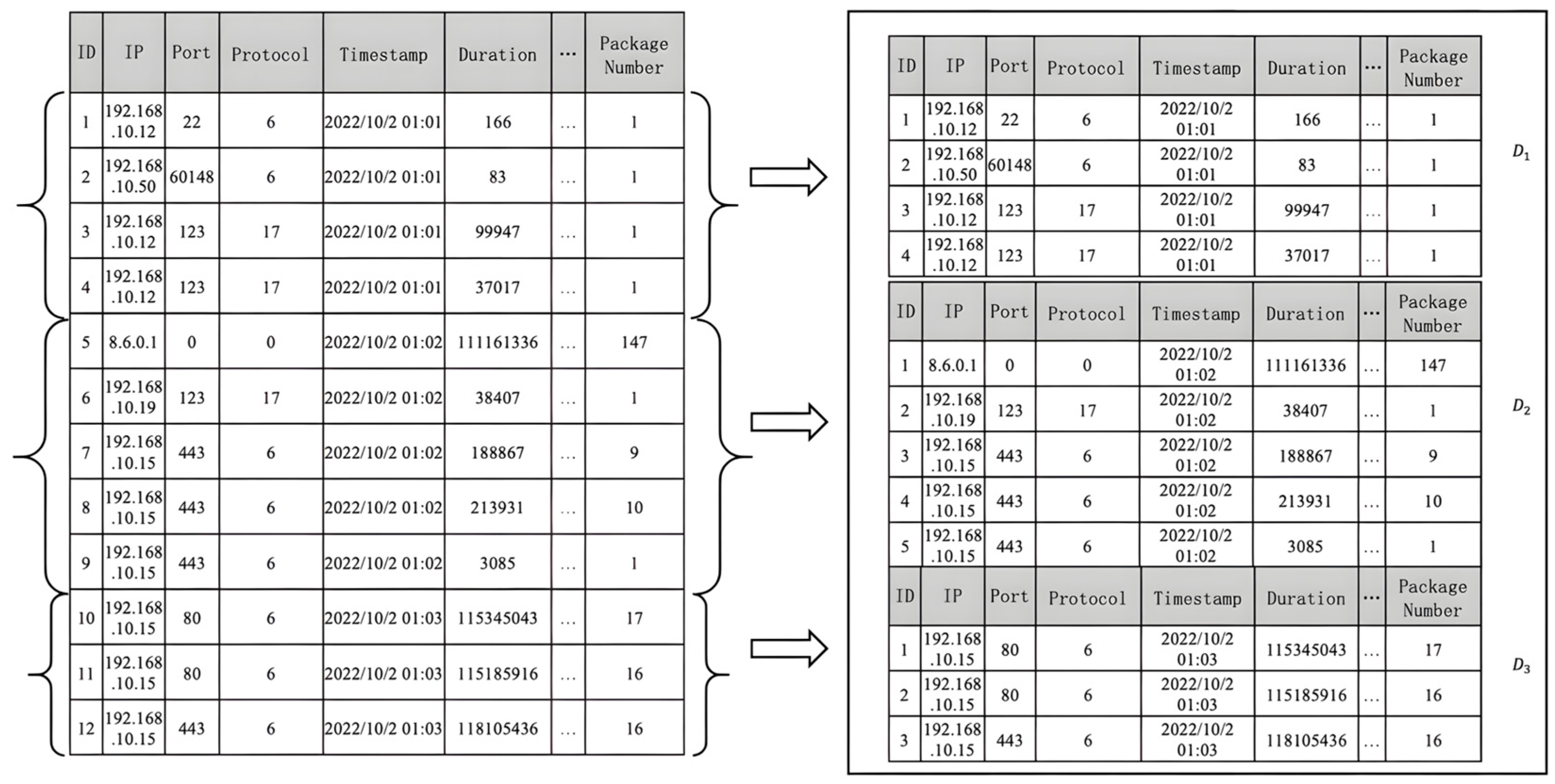
In Figure 6, consider the network traffic dataset with the timestamp features set as τ = [2022/10/2 01:01,2022/10/2 01:02,2022/10/2 01:03], timelen = 3, and D = 12. If we set the timestamp to 1, we can divide the dataset into three subsets: D 1 , D 2 and D 3 , based on the timestamp features. D 1 contains all the data with the timestamp “2022/10/2 01:01”, D 2 contains all the data with the timestamp “2022/10/2 01:02”, and D 3 contains all the data with the timestamp “2022/10/2 01:03”.

3.3.4. Rules of Graph Construction

Unlike conventional construction methods, this model introduces a novel approach for constructing time subgraphs based on event primary keys. This method involves dividing the dataset into subsets using the timestamp value and constructing a subgraph where network events serve as nodes and their correlation relationships are represented as edges.
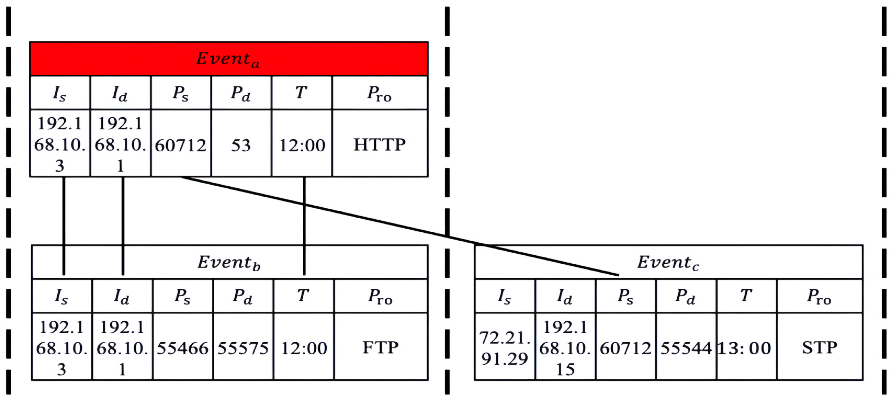
Figure 7 demonstrates the composition of network events, where the primary key of a network event is defined as E v e n t = I s , I d , P s , P d , T , P r o . I s represents the source IP address, I d represents the destination IP address, P s represents the source port, P d represents the destination port, T represents the timestamp, and P r o represents the protocol used in the communication (e.g., STP, HTTP, HTTPS, etc.). These six features collectively form the primary key that uniquely identifies a network communication behavior. In other words, a network event (Event) represents the occurrence of a message being sent from a source IP address ( I s ) to a destination IP address ( I d ) via a specific source port ( P s ) and destination port ( P d ) at a given timestamp ( T ) according to the rules defined by the protocol ( P r o ).
The construction of the graph involves using events as the nodes, and the correlation between nodes is utilized to establish edges. Since nodes are composed of multiple features, the strength of the correlation between them can vary. In Figure 8, for example, if we have three nodes: E v e n t a , E v e n t b , and E v e n t c , where E v e n t a and E v e n t b share the same source and destination IP addresses within the same time period, while E v e n t a and E v e n t c only share the same source port number, but occur at different time periods. In this scenario, when E v e n t a is identified as abnormal, E v e n t b , which shares more primary keys, becomes more suspicious due to the stronger correlation with E v e n t a .
The relationships between nodes in the graph can provide valuable information about the correlation and differences between them. These relationships can be used to describe the strength of correlation as well as highlight dissimilarities.
Based on the “device aggregation” and “activity aggregation” characteristics of network anomalies, we can summarize the correlation between nodes as follows:
  • When multiple nodes exhibit frequent communication patterns using the same source IP address, source port number, destination IP address, destination port number, and protocol within the same time period, the correlation between these nodes is strong and highly suspicious.
  • When multiple nodes frequently initiate communication over the same protocol but with different source IP addresses, source port numbers, and the same destination IP address and destination port number within the same time period, there is a possibility of “device aggregation”. In this case, the correlation between these nodes is weak but still suspicious.
  • When multiple nodes use the same source IP address and source port number to frequently initiate communication to different destination IP addresses, destination port numbers, and different protocols within the same time period, this behavior may not be obvious, but should not be ignored. The correlation between these nodes is the weakest among the three scenarios.
Based on the analysis, this model suggests establishing different correlation relationships between nodes in the same time period as edges. Three neighboring edge labels are defined as follows:
  • Strong Correlation: two nodes have the same source IP address, source port number, target IP address, target port number, and protocol in the same time period.
  • Moderate Correlation: two nodes have the same target IP address, target port number, and protocol in the same time period.
  • Weak Correlation: two nodes have the same source IP address and source port number in the same time period.
As Table 1 shows, these edge labels provide a way to represent the different levels of correlation between nodes, allowing for a more detailed description of the relationships in the graph.
The construction of edges is based on the neighboring edge labels. The process involves the following steps:
  • Determine if the two nodes are strongly correlated. If they do, they establish a “Strong Correlation” edge between them.
  • If the nodes do not have a “Strong Correlation”, determine if they are moderately correlated. If they do, establish a “Moderate Correlation” edge relationship between them.
  • If the nodes do not have a “Moderate Correlation”, determine if they are weakly correlated. If they do, establish a “Weak Correlation” edge relationship between them.
  • If none of the above conditions are met, there is no correlation between the nodes, and no edge relationship is established.
The characteristics of the neighboring edges are labeled accordingly and stored in the dictionary of neighboring edge labels E l . The dictionary consists of the three neighboring edge labels as the primary keys and the corresponding sets of neighboring nodes as the values.
By following these construction rules, an event key time subgraph can be constructed on each data subset, where the network events serve as graph nodes and the correlation relationships between them serve as edges.

3.4. EESAGE Algorithm

The construction of the event key time subgraphs allows for the extraction of rich feature information and structural information from network traffic data. However, this information cannot be directly utilized. To address this, the model proposes EESAGE, a graph representation learning algorithm that leverages neighboring-edge enhancement. EESAGE aims to learn embedding vectors for graph nodes, enabling effective anomaly detection in subsequent analysis.
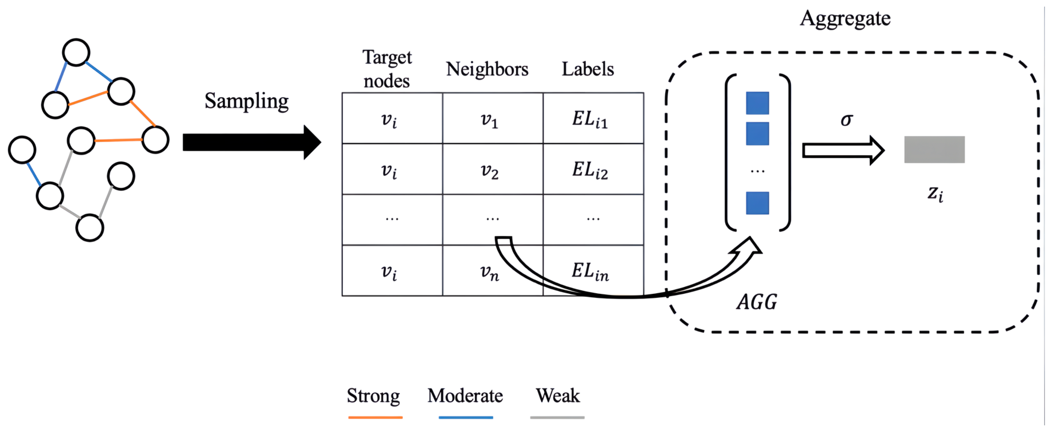
The algorithm consists of two main components: the neighboring-edge selection sampling algorithm and the neighboring-edge enhancement aggregation algorithm, as illustrated in Figure 9. In the neighboring-edge selection sampling algorithm, it selects and samples nodes in the graph based on their different neighboring edge labels. This step helps in identifying the relevant nodes that contribute to the anomaly detection process. The neighboring-edge enhancement aggregation algorithm takes into consideration the rich information contained in the neighboring edges and the discrepancies between them. It aggregates the features of nodes and their neighboring nodes while incorporating the neighboring edge labels as a feature. This process allows for the generation of a more accurate and effective node embedding vector.

3.4.1. Neighboring-Edge Selection Sampling Algorithm

Algorithm 2 outlines the process. For a given node v , its neighboring edge labels dictionary E v L stores the mapping relationships of three neighboring edge labels and their corresponding neighboring nodes. In the sampling process, the nodes v are initially sampled in the order of “Strong Correlation,” “Moderate Correlation,” and “Weak Correlation.” If the desired number of sampled nodes has not been reached, the nodes are added to the set of neighboring nodes N v using the expression:
N v N v v ,
The neighboring edge labels between two nodes are also recorded in the neighboring edge label matrix E L using the expression:
E l v v e l ,
where e l represents the neighboring edge labels between v and v . Sampling continues until the number of nodes in the set of neighboring nodes N v satisfies the desired sampling number ( sa_num ) or until all neighboring nodes have been sampled, in which case the sampling process is terminated using the “break” function.
Algorithm 2: Neighboring-edge selection sampling algorithm
Input:
node set V ;
neighboring edge labels dictionary E v l , v V ;
sampling number sa_num ;
Output:
neighborhood for node N v , v V ;
neighboring edge labels matrix E L v v , v V , v N v ;
1: for v   V do
2:  for e l = Weak ,   Moderate ,   Weak do
3:    n e i E v l e l ;
4:     for v n e i do
5:      if ( N ν < sa_num ) then
6:        N v N v v ;
7:        E L v v e l ;
8:      else
9:       break ();
10:     end if
11:    end for
12:  end for
13: end for
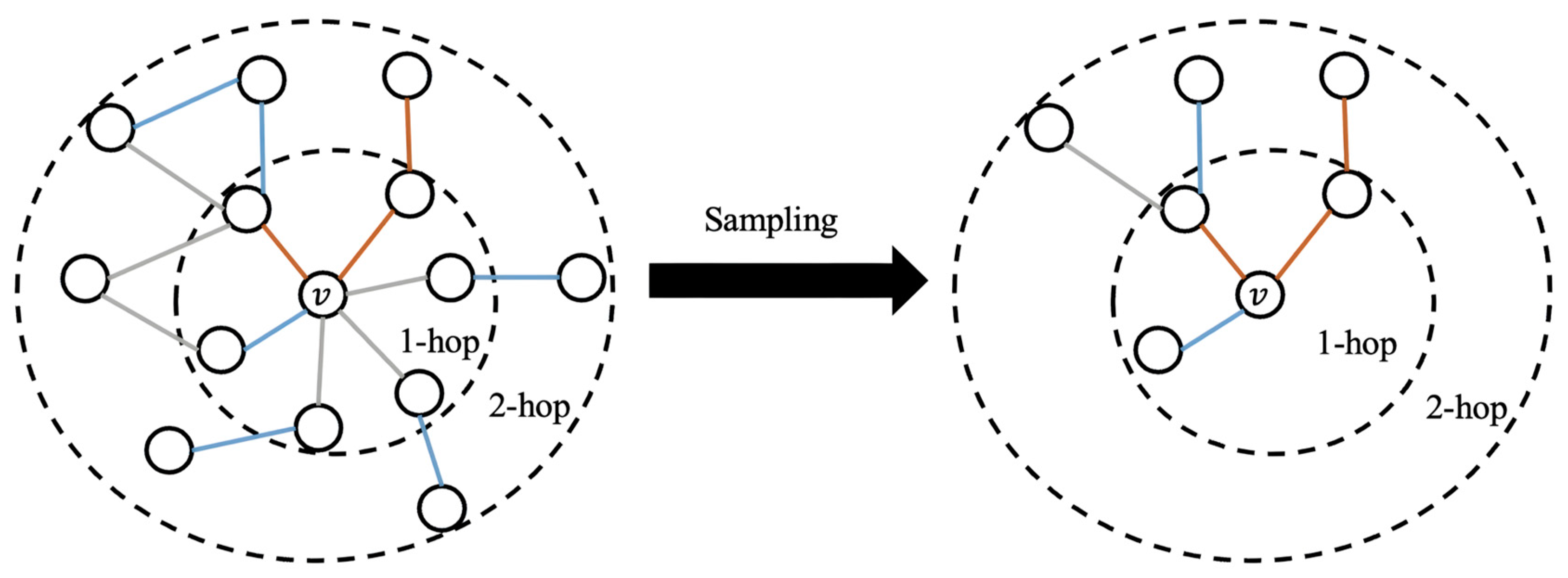
For instance, referring to Figure 10, when sampling the second-order neighboring node set of nodes v with a desired sample size of three, the neighboring nodes associated with the neighboring edge labeled “Strong Correlation” are sampled first. Subsequently, the neighboring nodes linked by the neighboring edge labeled “Moderate Correlation” and “Weak Correlation” are sampled until the desired sample size of three is achieved at each order.

3.4.2. Neighboring-Edge Enhancement Aggregation Algorithm

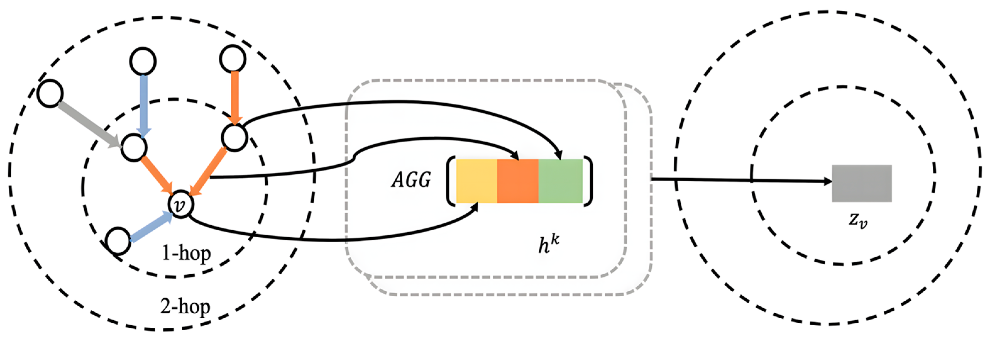
The neighboring nodes and the neighboring edge labels matrix of each node in the graph are sampled using the neighboring-edge selection algorithm, and they are then iteratively aggregated to obtain the final node embedding vectors. Illustrated in Figure 11, the neighboring-edge enhancement aggregation algorithm simultaneously combines the features of node v , its neighboring node features, and the neighboring edge label features to generate the corresponding embedding vector z v .
Specifically, Algorithm 3 illustrates the process of graph node aggregation for a single layer. The algorithm takes the set of nodes V , the set of node features X , the set of neighboring nodes N , and the set of neighboring edge labels E L as input. It also defines the aggregation depth K, the aggregation function A G G , the weight matrix W , and the activation function σ .
Algorithm 3: Neighboring-edge enhancement aggregation algorithm
Input:
node set V ;
node features X v , v V ;
neighborhood for node N v , v V ;
aggregation depth L ;
aggregation function A G G ;
weight matrix W ;
activation function σ ;
Output:
embedding vector z v , v V ;
1: h v 0 x v , v V
2: for l = 1 , L . do
3:  for v   V do
4:    C v l C O N C A T { h v l 1 E L v v , v N v } ;
5:    h C v l A G G h v l , v C v l ;
6:    h v l σ W l × C O N C A T h v l 1 , h C v L ;
7:  end for
8:   h v l h v l | h v l | 2 ;
9: end for
10: z v h v l , v V ;
In Algorithm 3, the first step is to concatenate the neighboring node features of node v with its corresponding neighboring edge label feature:
C v l C O N C A T ( { h v l 1 | | E L v v v N v } ) ,
where ( h v l 1 | | E L v v ) represents the concatenation of the neighboring node features of node v at layer l-1 and its corresponding neighboring edge label feature, resulting in the concatenated feature at layer l.
These concatenated features are then combined using the CONCAT function to obtain the set C v l , where each feature in C v l is aggregated using the AGG function. In this model, the mean aggregation function is employed, which can be expressed as follows:
h C v l A G G h u l , u C v l ,
In the next step, the CONCAT operation is performed between the aggregated and combined features h C v l and the node features h v l 1 . The resulting features are then multiplied by the weight matrix W l at layer l and passed through the activation function σ. Line 8 represents the normalization operation, and as a result, the embedding vector z v of node v is obtained.

3.5. Detection Algorithm

After obtaining the embedding vectors of graph nodes, the next step is to evaluate and classify them to detect abnormal nodes. This model determines whether a node is abnormal or not by comparing its embedding vector with a detection threshold (threshold). Let Z be the set of node embedding vectors, and let the labels of nodes be denoted as C 1 and C 2 , indicating normal and abnormal, respectively. For a given node v, its label C v can be determined using the following equation:
C v = C 1 Z ν t h r e s h o l d C 2 Z ν t h r e s h o l d ,
Therefore, the selection of the detection threshold is crucial for accurate anomaly detection. Setting the threshold too low may result in the neglect of abnormal network data, while setting it too high may lead to misclassifying normal data as abnormal. To address this issue, this model employs an adaptive threshold selection strategy based on the training data. The strategy involves selecting all nodes labeled as normal from the training data, obtaining their corresponding embedding vectors, and selecting the minimum value among these embedding vectors as the initial detection threshold. This ensures that the initial threshold has high accuracy and effectively distinguishes normal nodes from abnormal ones. The formula for calculating the initial detection threshold is as follows:
t h r e s h o l d = min z Z B z ,
where Z B represents the set of embedding vectors of normal nodes in the training data. The initial detection threshold is then adjusted based on further analysis of experimental results to achieve the best detection outcome.

4. Experiments

4.1. Dataset

This experiment validates the model using web traffic data generated on different dates from the CIC-IDS2017 dataset [22]. This dataset contains the abstract behavior of 25 users over 5 days, including various attack types such as DoS, DDoS, Heartbleed, web attacks, infiltration, Botnet, and brute-force attacks. Compared to older datasets such as KDD’99 or NSL-KDD, CIC-IDS2017 provides realistic traffic patterns, comprehensive network features, temporal continuity, and contemporary attack scenarios, making it a suitable benchmark for validating the performance, robustness, and adaptability of the proposed model. For the experiment, the model focuses on the network traffic datasets of Tuesday, Wednesday, Thursday, and Friday, as the Monday datasets are all normal. Table 2 provides an overview of these datasets.

4.2. Experimental Setting

Environment: The experiment is conducted on a macOS (Monterey) system with an 8-core Apple M1 and 16 GB RAM. The experimental code is implemented in a Python 3.8 environment, utilizing the PyTorch 2.2.1 library for the implementation of the EESAGE algorithm.
Hyperparameters: In this experiment, a batch training method is utilized. The model is trained for 20 epochs, and the batch size is determined based on the ETG generated at different timestamps to ensure that the batches are approximately the same size when training different ETGs in batches. The Adam optimizer is used with a learning rate of 0.001.
The ratio of the training set, validation set, and test set is set to 2:4:4, aiming to utilize as few training samples as possible for training. The sampling step is set to 1, and a total of 10 samples are taken. The CrossEntropyLoss function is employed to calculate the loss value, the Mean function is used as the aggregation function for node features, and the ReLU function is applied as the nonlinear activation function.
Initial timestamp: The initial timestamp should be determined based on the specific network environment. In this experiment, a reference is made to the Cisco Annual Cybersecurity Report 2021 [23], which states that approximately 27% of global network traffic is flagged as anomalous. These anomalies include spam, malware, phishing, and other types of traffic. Cisco monitors and analyzes network traffic worldwide using its network security products, such as Intrusion Prevention System (IPS), Security Information and Event Management (SIEM), and Cloud Security Services.
Based on the data provided by Cisco, the ratio of network anomaly data to the total data volume (radio) is set to 27% in this experiment. Additionally, by analyzing the data situation, a value of α is set to 2. The initial timestamp for the Tuesday, Wednesday, Thursday, and Friday datasets was determined to be 65 min, 68 min, 65 min, and 53 min, respectively.
Further analysis and experimentation were conducted to adjust the timestamp at 5-min intervals based on the observed experimental results. The detailed analysis process is not repeated here. Ultimately, the experimental results obtained at different timestamps were compared to determine the best result.
Initial Threshold: After learning from the normal nodes in the training data, their corresponding embedding vector sets are obtained. Then, the minimum value in the embedding vector set is calculated, resulting in initial detection thresholds of 0.6, 0.6, 0.8, and 0.7 for the Tuesday, Wednesday, Thursday, and Friday datasets, respectively.
Subsequently, an analysis of the experimental results under the initial detection thresholds reveals that adjusting them by 0.01 does not significantly affect the results. Therefore, after experimenting with random values, an interval of 0.1 is chosen for adjusting the thresholds. Finally, different detection thresholds are experimentally compared to determine the optimal determination threshold.
To ensure a fair and comprehensive comparison, the proposed model is evaluated against three categories of representative algorithms:
(1)
Traditional machine learning methods: KNN, RF, CART, Adaboost, QDA, which rely on feature engineering and serve as classical baselines. These algorithms are widely used in network anomaly detection literature and provide benchmarks to evaluate the improvement brought by deep and graph-based models.
(2)
Deep learning and hybrid optimization methods: including models combining LSTM, attention mechanisms, or meta-heuristic algorithms such as SSA and H2GWO. They are selected because they represent state-of-the-art approaches that can capture temporal dependencies and complex nonlinear patterns in network traffic data.
(3)
Graph-based anomaly detection models: including recent works such as the hyperbolic embedding GNN and the continual-learning-based EL-GNN, which are chosen to assess performance in capturing relational and structural dependencies inherent in network traffic.
These comparison algorithms represent different mainstream paradigms for network anomaly detection, covering both shallow and deep architectures, as well as recent graph representation approaches. Their inclusion allows a balanced evaluation of performance, robustness, and adaptability against the proposed ETG-EESAGE model.

4.3. Results and Discussion

This subsection provides a detailed presentation of the experimental results on different datasets. Due to the potential variations in features and data noise across different environments, separate experiments and analyses are conducted for each dataset.
The experiments begin by setting the initial timestamp and detection threshold specific to each dataset. The timestamps are adjusted in 5-min intervals, while the detection thresholds are adjusted in 0.1 intervals. This leads to multiple combinations of timestamp and detection threshold. Each combination is subjected to experimental analysis and comparison to determine the optimal results for that particular dataset.
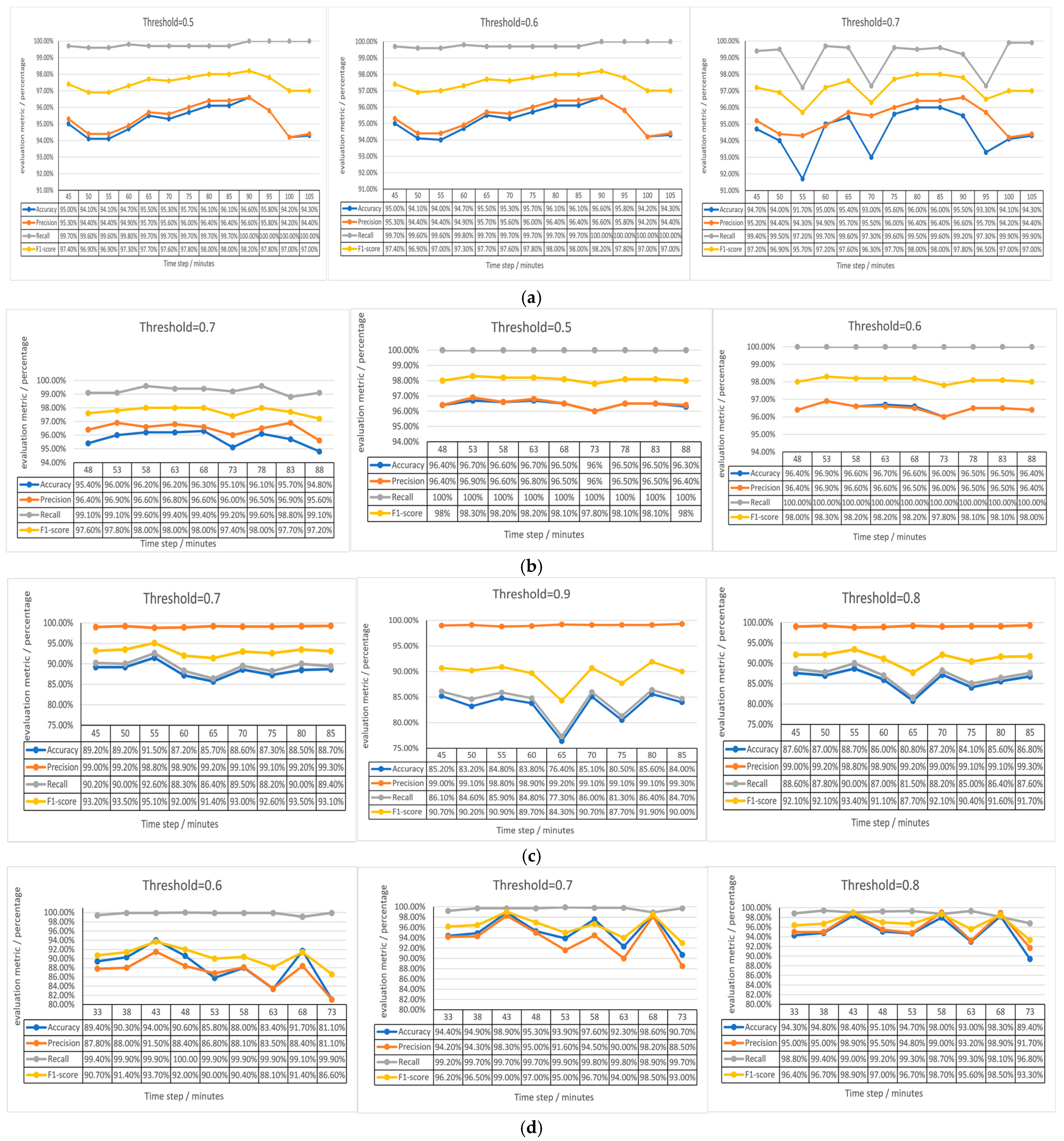
As shown in Figure 12a on the Tuesday dataset, the curves of evaluation metrics exhibit similar fluctuation trends when the detection thresholds are set to 0.5 and 0.6. These curves gradually increase with increasing timestamps and reach their peak performance at a timestamp of 90 min, achieving values of 96.6%, 96.5%, 100%, and 98.2%, respectively. After reaching the peak, the evaluation metrics gradually decrease. This indicates that at a timestamp of 90 min, the choice of detection threshold (0.5 or 0.6) has less impact on the results.
When the detection threshold is set to 0.7, there are noticeable fluctuations in the curves of the evaluation metrics across different timestamps. The best performance is observed at a timestamp of 85 min, with values of 96.0%, 96.4%, 99.6%, and 98.0% for the evaluation metrics. Afterward, all the evaluation metrics, except for the recall rate, show a decreasing trend.
As shown in Figure 12b, on the Wednesday dataset, when the detection thresholds were set to 0.5 and 0.6, the fluctuations in the curves of the evaluation metrics for the change in timestamp were more similar. All the evaluation metrics reached their peak values at a timestamp of 53 min, achieving 96.7%, 96.9%, 100%, and 98.3% for each evaluation metric. Therefore, at a timestamp of 53 min, setting a detection threshold of 0.5 or 0.6 did not significantly affect the results.
When the detection threshold was set to 0.7, the curves of each evaluation metric showed more variation with increasing timestamps. The best performance was observed at a timestamp of 68 min, with values of 96.3%, 96.6%, 99.4%, and 98% for each evaluation metric.
As shown in Figure 12c, on the Thursday dataset, the accuracy and recall rates exhibited similar performance at different timestamps when the detection threshold was set to 0.7. However, the accuracy rate generally performed better. When considering all the metrics together, a clear peak value was observed at a timestamp of 55 min, with the combined evaluation metrics achieving 91.5%, 98.8%, 92.6%, and 95.1%.
At detection threshold values of 0.8 and 0.9, the curves of each evaluation metric were similar. For a detection threshold of 0.8, the best performance was observed for the combined evaluation metrics at a timestamp of 55 min. For a detection threshold of 0.9, the best performance of the evaluation metrics was distributed across different timestamps. Specifically, the highest accuracy rate was 85.2% at a timestamp of 45 min, the highest precision rate was 99.3% at a timestamp of 85 min, and the recall rate and F1-score reached 86.4% and 91.9%, respectively, at a timestamp of 80 min.
As shown in Figure 12d, on the Friday dataset, at a detection threshold of 0.6, the recall rate was consistently higher at different timestamps compared to the other evaluation metrics. The curves of the other evaluation metrics exhibited significant fluctuations, reaching their peak values at a timestamp of 43 min with 94%, 91.5%, 99.9%, and 93.4%.
At a detection threshold of 0.7, the accuracy and F1-score results showed relatively similar variations at different timestamps, while the recall results remained consistently higher than the other evaluation metrics. Fluctuations were observed in each evaluation metric across different timestamps, with peaks and valleys. Among them, the best performance in terms of the comprehensive evaluation metrics was achieved at a timestamp of 43 min, with values of 98.9%, 98.3%, 99.7%, and 99% for accuracy, precision, recall, and F1-score, respectively.
At a detection threshold of 0.8, the accuracy, precision, and F1-score results exhibited consistent variations at different timestamps. Similarly, each evaluation metric still showed fluctuations, with peak values of 98.4%, 98.9%, 99.0%, and 98.9% at a timestamp of 43 min, respectively.
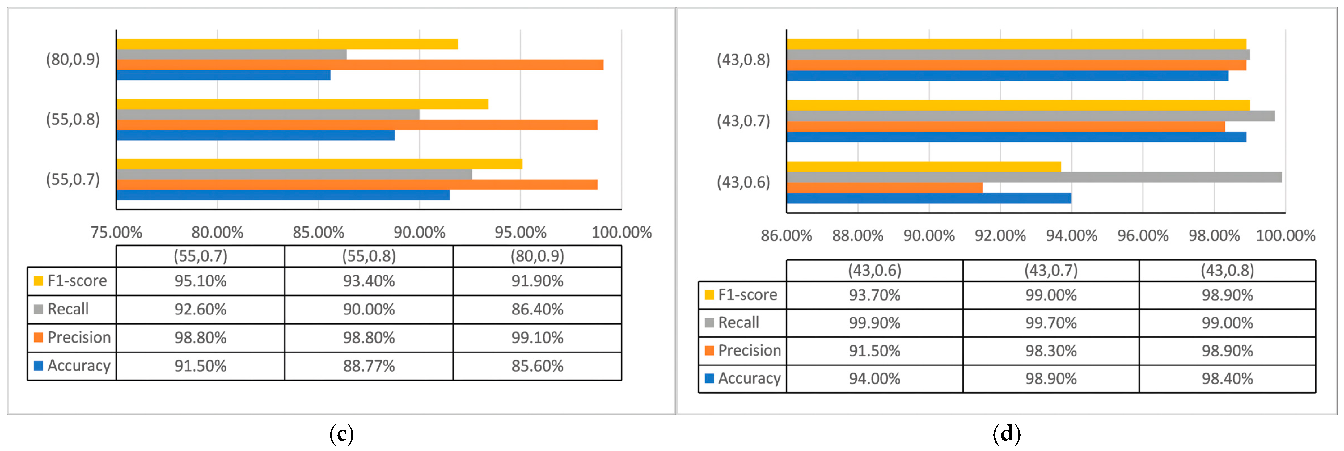
The optimal results with different parameters on each dataset were compared. As shown in Figure 13a, in the Tuesday dataset, the best performing timestamps for the combined evaluation metrics were 90, 90, and 85 min for detection thresholds of 0.5, 0.6, and 0.7, respectively. When comparing the combinations (90,0.5), (90,0.6), and (85,0.7), it was found that the results for (90,0.5) and (90,0.6) were the same, and both were higher than the results for (85,0.7). Therefore, on the Tuesday dataset, the best performance for each evaluation metric was achieved when the timestamp was set to 90 min, and the detection thresholds were 0.5 and 0.6.
As shown in Figure 13b, on the Wednesday dataset, the best performance of the combined evaluation metrics was achieved at timestamps of 53, 53, and 68 min for detection thresholds of 0.5, 0.6, and 0.7, respectively. Comparing the combinations (53,0.5), (53,0.6), and (68,0.7), it was found that (53,0.5) and (53,0.6) were higher than (68,0.7) for all evaluation metrics, and the difference between them was not significant. However, (53,0.6) showed slightly better accuracy than (53,0.5). Therefore, on the Wednesday dataset, each evaluation metric performed best when the timestamp was set to 53 min, and the detection threshold was 0.6.
As shown in Figure 13c, on the Thursday dataset, the best performing timestamps for the combined evaluation metrics were 55 min, 55 min, and 80 min at detection threshold values of 0.7, 0.8, and 0.9, respectively. A comparison of the combined values (55,0.7), (55,0.8), and (80,0.9) revealed similar accuracy results, while (55,0.7) performed the best in terms of accuracy, recall, and F1-score. Thus, in the experiments for the Thursday dataset, the model performed best in terms of overall evaluation metrics with a timestamp of 55 min and a detection threshold of 0.7.
As shown in Figure 13d, on the Friday dataset, the model achieved the best performance in terms of evaluation metrics for different detection thresholds of 0.6, 0.7, and 0.8 with a timestamp of 43 min. Furthermore, comparing the combinations (43,0.6), (43,0.7), and (43,0.8), the results for (43,0.7) and (43,0.8) were closer, while (43,0.6) stood out in terms of recall, although the difference was not significant compared to the other two combinations. Considering all the evaluation metrics, the model performed best on the Friday dataset when the timestamp was set to 43 min and the detection threshold was set to 0.7.

4.4. Sensitivity and Robustness Analysis of the Detection Threshold

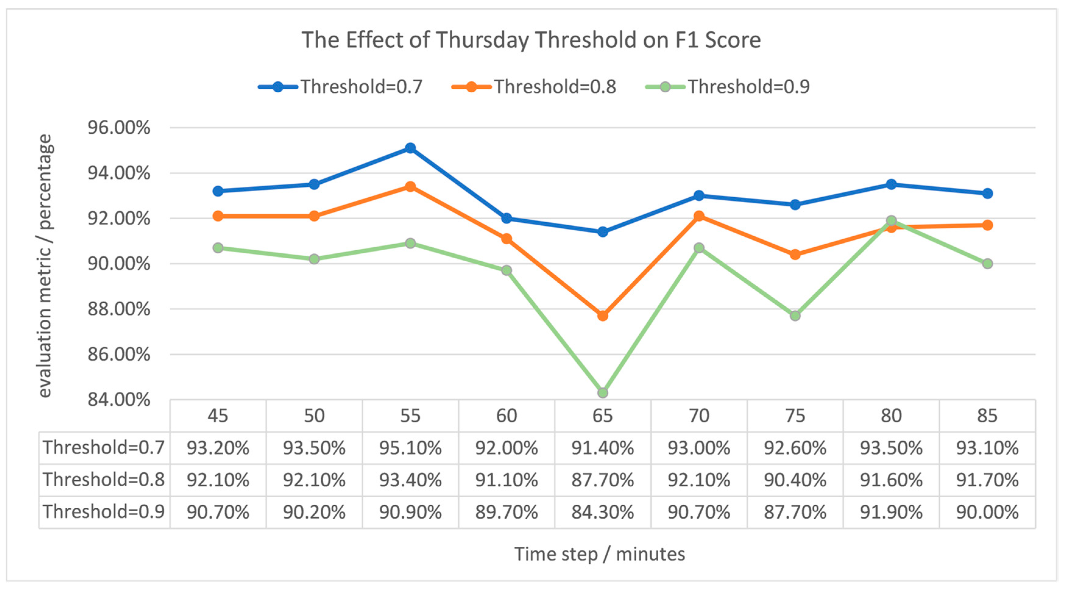
To evaluate the impact of the detection threshold on model performance and verify its robustness, we conducted a systematic sensitivity analysis. Using the Thursday dataset as an example, we tested three different detection thresholds: 0.7, 0.8, and 0.9, over a time step range of 45 to 85 min. The F1 score was used as the core evaluation metric. The results are shown in Figure 14. The analysis demonstrates that the model performance exhibits robustness to the choice of threshold. Specifically, around the 55-min time step, the model maintains high F1 scores, exceeding 93% across all thresholds, forming a plateau. This demonstrates that within this optimal operating range, the model’s classification performance is not dependent on a single optimal threshold and is insensitive to small changes in the threshold parameter. This significantly enhances the model’s practicality and adaptability in real-world deployments. This analysis provides empirical evidence for selecting robust threshold parameters, reducing the difficulty of parameter tuning and operational costs in real-world scenarios.

4.5. Compared with Other Algorithms

This section compares the experimental results of different types of detection methods with the proposed model, including traditional machine learning methods, deep learning methods, and heuristic optimization methods, to comprehensively evaluate the performance differences in various methods in anomaly detection tasks, as shown in Table 3. Goryunov et al. [24], who optimized the data preprocessing and sampling process, adjusted training parameters based on different datasets and attack type criteria to obtain the best-performing classifier for network anomaly detection. Among the ten machine learning algorithms optimized in their study, five supervised learning algorithms with better results are selected for comparison in this subsection. These algorithms include: KNN, RF, CART, Adaboost, and QDA.
Zhang et al. [25] proposed an anomaly detection model that combines hierarchical hybrid grey wolf optimization (H2GWO) with a lightweight Transformer. H2GWO uses simulated annealing and differential evolution to enhance search capabilities, while Transformer reduces complexity through convolutional time windows and attention mechanisms. Shyaa et al. [26] introduced a GPC classification framework using three Online Sequential Extreme Learning Machine (OSELM) variants to handle concept drift in data streams and designed adaptive mechanisms for data balancing and classifier updates. Hu et al. [27] proposed an online anomaly detection method based on dual adaptive windows and Hoeffding Tree classifiers to dynamically adjust drift sensitivity and prediction accuracy. Idrissi et al. [28] proposed a distributed anomaly detection method based on an autoencoder (AE) and federated learning (FL). The encoder is trained locally and its weights are aggregated on a central server, enabling privacy-preserving intrusion detection. Dash et al. [29] proposed a Long Short-term Memory (LSTM) anomaly detection model combined with an attention mechanism, and optimized the model parameters through the Salp Swarm algorithm (SSA), effectively improving the modeling and classification capabilities of network traffic. Zhang et al. [30] proposed a graph neural network-based anomaly detection model that embeds network data into hyperbolic space and optimizes edge weights via a gain factor, effectively enhancing the representation of relational anomalies in network structures. Nguyen [31] proposed a continual-learning-based graph neural network (EL-GNN) that effectively mitigates catastrophic forgetting in intrusion detection systems, enabling adaptive and incremental learning for evolving network attacks.
After comparing the results of other algorithms with the average evaluation metrics of the proposed model, we observe that the proposed model performs well in terms of accuracy, recall, and F1-score, demonstrating competitive performance compared with both traditional and deep learning-based approaches. Specifically, compared with traditional machine learning models such as KNN, RF, and CART, the proposed ETG-EESAGE model achieves a higher overall F1-score, indicating stronger stability and robustness in complex anomaly detection scenarios. Compared with deep learning methods such as SSA-LSTM and Fed-ANIDS, our model maintains superior recall and precision balance, showing its ability to capture abnormal behaviors more effectively without overfitting to specific attack types. Moreover, when compared to graph-based detection methods like DGI + GAT and EL-GNN, the ETG-EESAGE framework further enhances relational feature representation by integrating edge label semantics into the aggregation process, achieving more accurate characterization of temporal and structural dependencies in network traffic.
However, there remains a slight deficiency in accuracy, which could be attributed to the model’s feature selection process and the limited number of training samples. While the current model demonstrates overall superior performance, there is still potential for further optimization. For instance, exploring more advanced and adaptive feature selection mechanisms could improve the ability to extract more discriminative features. Additionally, expanding the dataset with more diverse and representative samples could enhance the model’s generalization capability and robustness in detecting anomalies across varying network environments.

5. Conclusions and Future Work

In this paper, we propose a novel network anomaly detection model that effectively captures temporal and structural characteristics of network traffic, which begins by preprocessing the raw network data to obtain a refined network traffic dataset. A novel temporal subgraph construction method is then adopted, which divides the dataset into multiple subsets based on timestamp features and constructs an event-critical temporal subgraph (ETG) for each subset. To enhance node representations, we employ the Edge-Enhanced Sampling and Aggregation (EESAGE) algorithm, which combines edge selection sampling and edge-enhanced aggregation. It captures precise inter-node correlations and edge heterogeneity, generating rich embeddings without requiring deep or computationally intensive aggregation layers. Finally, a detection algorithm using a threshold is applied to determine anomalous nodes. The model leverages the “device aggregation” and “activity aggregation” characteristics of network anomalies to effectively capture feature and structural information, leading to improved anomaly detection performance while reducing costs. Experimental evaluations on the CIC-IDS2017 dataset demonstrate that ETG-EESAGE achieves an average accuracy of 95.5%, precision of 97.9%, recall of 97.3%, and F1-score of 97.7%, confirming its strong detection capability and robustness across different traffic scenarios.
In terms of future explorations, there are three promising directions for further research in network anomaly detection. The first direction involves building hyper-graphs on large-scale data to address the challenges posed by complex and extensive datasets, enabling more effective modeling and improved detection performance. The second direction focuses on the development of lightweight models that allow anomaly detection at endpoints or on mobile devices, aiming to protect data privacy while maintaining high detection efficiency. These models are designed with low computational requirements and minimal resource consumption, making them suitable for deployment on resource-constrained devices. A third promising direction is the integration of reinforcement learning techniques with the proposed ETG-EESAGE framework. Although a direct comparison with recent reinforcement learning-based methods is not feasible on the current dataset, incorporating reinforcement learning could enhance the adaptability and performance of the model in dynamic network environments, offering a valuable avenue for extending ETG-EESAGE to more complex and large-scale scenarios while maintaining efficiency and scalability. Enterprise-level network anomaly detection also warrants attention. Future research will focus on extracting richer features from assets and network traffic—such as device updates, connection counts, TCP/UDP flows, and open ports—while incorporating user behavior analysis to build more comprehensive detection systems for complex enterprise networks.

Author Contributions

Conceptualization, B.Q.; Writing—original draft preparation, S.Z. and J.Z.; Writing—review and editing, B.Q., S.Z., J.Z. and L.T. All authors have read and agreed to the published version of the manuscript.

Funding

This research was funded by Guangdong University of Science and Technology, grant number GKY-2023BSQD-15.

Data Availability Statement

The original contributions presented in this study are included in the article. Further inquiries can be directed to the corresponding author.

Conflicts of Interest

The authors declare no conflicts of interest.

References

  1. Chandola, V.; Banerjee, A.; Kumar, V. Anomaly Detection: A Survey. ACM Comput. Surv. 2009, 41, 15. [Google Scholar] [CrossRef]
  2. Hawkins, D.M. Identification of Outliers; Springer: Berlin/Heidelberg, Germany, 1980; Volume 11. [Google Scholar]
  3. Liu, L.; Chen, B.; Qu, B.; He, L.; Qiu, X. Data Driven Modeling of Continuous Time Information Diffusion in Social Networks. In Proceedings of the 2017 IEEE Second International Conference on Data Science in Cyberspace (DSC), Shenzhen, China, 26–29 June 2017; IEEE: New York, NY, USA, 2017; pp. 655–660. [Google Scholar]
  4. Khalil, I.; Yu, T.; Guan, B. Discovering Malicious Domains through Passive DNS Data Graph Analysis. In Proceedings of the 11th ACM on Asia Conference on Computer and Communications Security, Xi’an, China, 30 May–3 June 2016; pp. 663–674. [Google Scholar]
  5. Qu, B.; Li, C.; Van Mieghem, P.; Wang, H. Ranking of Nodal Infection Probability in Susceptible-Infected-Susceptible Epidemic. Sci. Rep. 2017, 7, 9233. [Google Scholar] [CrossRef] [PubMed]
  6. Hu, Z.; Qu, B.; Li, X.; Li, C. An Encrypted Traffic Classification Framework Based on Higher-Interaction-Graph Neural Network. In Proceedings of the Australasian Conference on Information Security and Privacy, Sydney, NSW, Australia, 15–17 July 2024; Springer: Berlin/Heidelberg, Germany, 2024; pp. 383–403. [Google Scholar]
  7. Liu, Z.; Chen, C.; Yang, X.; Zhou, J.; Li, X.; Song, L. Heterogeneous Graph Neural Networks for Malicious Account Detection. In Proceedings of the 27th ACM International Conference on Information and Knowledge Management, Torino, Italy, 22–26 October 2018; pp. 2077–2085. [Google Scholar]
  8. Ding, K.; Li, J.; Bhanushali, R.; Liu, H. Deep Anomaly Detection on Attributed Networks. In Proceedings of the 2019 SIAM International Conference on Data Mining, Calgary, AB, Canada, 2–4 May 2019; SIAM: Philadelphia, PA, USA, 2019; pp. 594–602. [Google Scholar]
  9. Goldman, A.; Cohen, I. Anomaly Detection Based on an Iterative Local Statistics Approach. Signal Process. 2004, 84, 1225–1229. [Google Scholar] [CrossRef]
  10. Ye, N.; Chen, Q. An Anomaly Detection Technique Based on a Chi-Square Statistic for Detecting Intrusions into Information Systems. Qual. Reliab. Eng. Int. 2001, 17, 105–112. [Google Scholar] [CrossRef]
  11. Wang, J.; Hong, X.; Ren, R.; Li, T. A Real-Time Intrusion Detection System Based on PSO-SVM. In Proceedings of the 2009 International Workshop on Information Security and Application (IWISA 2009), Busan, Republic of Korea, 25–27 August 2009; Academy Publisher: London, UK, 2009; p. 319. [Google Scholar]
  12. Su, M.-Y. Real-Time Anomaly Detection Systems for Denial-of-Service Attacks by Weighted k-Nearest-Neighbor Classifiers. Expert Syst. Appl. 2011, 38, 3492–3498. [Google Scholar] [CrossRef]
  13. Li, Y.; Ma, R.; Jiao, R. A Hybrid Malicious Code Detection Method Based on Deep Learning. Int. J. Secur. Its Appl. 2015, 9, 205–216. [Google Scholar] [CrossRef]
  14. Schlegl, T.; Seeböck, P.; Waldstein, S.M.; Schmidt-Erfurth, U.M.; Langs, G. Unsupervised Anomaly Detection with Generative Adversarial Networks to Guide Marker Discovery. In Proceedings of the Information Processing in Medical Imaging, Boone, NC, USA, 25–30 June 2017. [Google Scholar]
  15. Liu, Y.; Wang, X.; Qu, B.; Zhao, F. ATVITSC: A Novel Encrypted Traffic Classification Method Based on Deep Learning. IEEE Trans. Inf. Forensics Secur. 2024, 19, 9374–9389. [Google Scholar] [CrossRef]
  16. Liu, F.; Wen, Y.; Zhang, D.; Jiang, X.; Xing, X.; Meng, D. Log2vec: A Heterogeneous Graph Embedding Based Approach for Detecting Cyber Threats within Enterprise. In Proceedings of the 2019 ACM SIGSAC Conference on Computer and Communications Security, London, UK, 11–15 November 2019; pp. 1777–1794. [Google Scholar]
  17. Cai, L.; Chen, Z.; Luo, C.; Gui, J.; Ni, J.; Li, D.; Chen, H. Structural Temporal Graph Neural Networks for Anomaly Detection in Dynamic Graphs. In Proceedings of the 30th ACM International Conference on INFORMATION & Knowledge Management, Virtual, 1–5 November 2021; pp. 3747–3756. [Google Scholar]
  18. Xiao, G.; Tong, H.; Shu, Y.; Ni, A. Spatial-Temporal Load Prediction of Electric Bus Charging Station Based on S2TAT. Int. J. Electr. Power Energy Syst. 2025, 164, 110446. [Google Scholar] [CrossRef]
  19. Zhang, S.; Xi, P.; Jiang, M.; Zhang, G.; Cheng, D. Latent Representation Learning for Attributed Graph Anomaly Detection. ACM Trans. Knowl. Discov. Data 2025, 19, 1–22. [Google Scholar] [CrossRef]
  20. Zhou, Z.; Abawajy, J. Reinforcement Learning-Based Edge Server Placement in the Intelligent Internet of Vehicles Environment. IEEE Trans. Intell. Transp. Syst. 2025; early access. [Google Scholar] [CrossRef]
  21. Kurniabudi, K.; Stiawan, D.; Darmawijoyo, D.; Idris, M.Y.B.; Kerim, B.; Budiarto, R. Important Features of CICIDS-2017 Dataset for Anomaly Detection in High Dimension and Imbalanced Class Dataset. Indones. J. Electr. Eng. Inform. 2021, 9, 498–511. [Google Scholar] [CrossRef]
  22. Sharafaldin, I.; Lashkari, A.H.; Ghorbani, A.A. Toward Generating a New Intrusion Detection Dataset and Intrusion Traffic Characterization. ICISSp 2018, 1, 108–116. [Google Scholar]
  23. Cisco Annual Internet Report (2018–2023) White Paper; Cisco Systems, Inc.: San Jose, CA, USA, 2019.
  24. Goryunov, M.N.; Matskevich, A.G.; Rybolovlev, D.A. Synthesis of a Machine Learning Model for Detecting Computer Attacks Based on the Cicids2017 Dataset. Proc. Inst. Syst. Program. RAS 2020, 32, 81–94. [Google Scholar] [CrossRef] [PubMed]
  25. Zhang, Y.; Zhao, H.; Liu, X.; Cui, Z.; Tian, Y.; Du, Y. Network Intrusion Detection Based on Layered Hybrid Grey Wolf Algorithm and Lightweight Transformer. In Proceedings of the 2025 8th International Conference on Advanced Electronic Materials, Computers and Software Engineering (AEMCSE), Nanjing, China, 9–11 May 2025; pp. 319–322. [Google Scholar]
  26. Shyaa, M.A.; Zainol, Z.; Abdullah, R.; Anbar, M.; Alzubaidi, L.; Santamaría, J. Enhanced Intrusion Detection with Data Stream Classification and Concept Drift Guided by the Incremental Learning Genetic Programming Combiner. Sensors 2023, 23, 3736. [Google Scholar] [CrossRef] [PubMed]
  27. Hu, X.; Ma, D.; Wang, W.; Liu, F. Dual Adaptive Windows Toward Concept-Drift in Online Network Intrusion Detection. In Proceedings of the International Conference on Computational Science, Singapore, 7–9 July 2025; Springer: Berlin/Heidelberg, Germany, 2025; pp. 210–224. [Google Scholar]
  28. Idrissi, M.J.; Alami, H.; Mahdaouy, A.E.; Mekki, A.E.; Oualil, S.; Yartaoui, Z.; Berrada, I. Fed-ANIDS: Federated Learning for Anomaly-Based Network Intrusion Detection Systems. Expert Syst. Appl. 2023, 234, 121000. [Google Scholar] [CrossRef]
  29. Dash, N.; Chakravarty, S.; Rath, A.K.; Giri, N.C.; AboRas, K.M.; Gowtham, N. An Optimized LSTM-Based Deep Learning Model for Anomaly Network Intrusion Detection. Sci. Rep. 2025, 15, 1554. [Google Scholar] [CrossRef] [PubMed]
  30. Zhang, H.; Zhou, Y.; Xu, H.; Shi, J.; Lin, X.; Gao, Y. Graph Neural Network Approach with Spatial Structure to Anomaly Detection of Network Data. J. Big Data 2025, 12, 105. [Google Scholar] [CrossRef]
  31. Nguyen, T.-T.; Park, M. EL-GNN: A Continual-Learning-Based Graph Neural Network for Task-Incremental Intrusion Detection Systems. Electronics 2025, 14, 2756. [Google Scholar] [CrossRef]
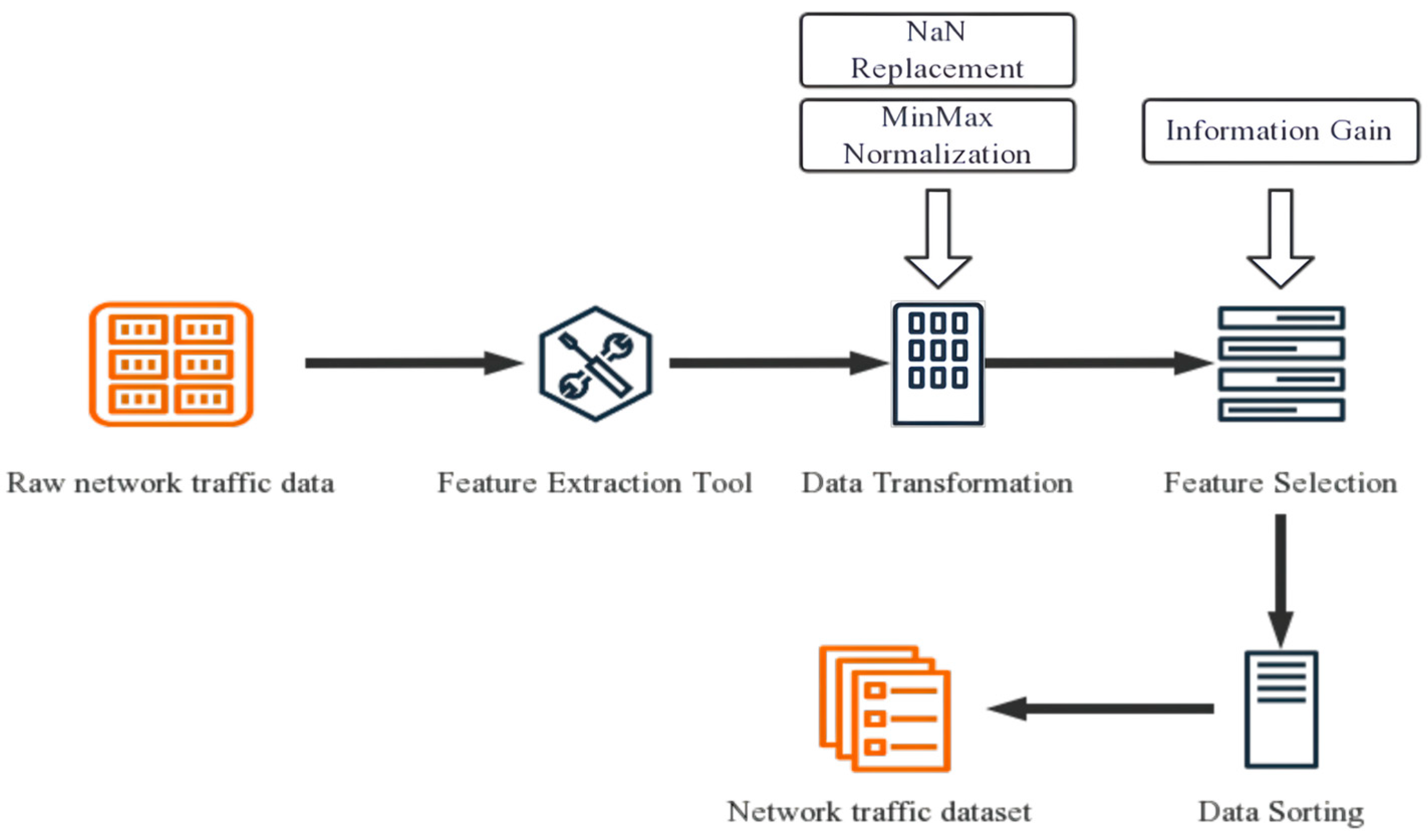
Figure 2. Workflow of pre-processing.
Symmetry 17 01976 g002
Figure 3. Process of ETG construction.
Symmetry 17 01976 g003
Figure 4. Features of device aggregation. (a) Normal user sessions are concentrated on one or two devices with a single IP. (b) Malicious sessions originate from numerous IPs to launch frequent, obfuscated attacks.
Symmetry 17 01976 g004
Figure 5. Features of activity aggregation. (a) A normal environment shows stable long-term patterns in device and IP distribution. (b) Malicious activity is time-constrained, causing a concentrated surge of IPs (e.g., at t 4 and t 5 ) that forms “activity aggregation”.
Symmetry 17 01976 g005
Figure 6. Example of dividing subsets.
Symmetry 17 01976 g006
Figure 7. Definition of node.
Symmetry 17 01976 g007
Figure 8. Differences in correlation between nodes.
Symmetry 17 01976 g008
Figure 9. Workflow of the EESAGE algorithm.
Symmetry 17 01976 g009
Figure 10. Example of Sampling.
Symmetry 17 01976 g010
Figure 11. Example of aggregating.
Symmetry 17 01976 g011
Figure 12. Experimental results (from Tuesday to Friday). (a) Tuesday: Model performance under different detection thresholds. (b) Wednesday: Model performance under different detection thresholds. (c) Thursday: Model performance under different detection thresholds. (d) Friday: Model performance under different detection thresholds.
Symmetry 17 01976 g012
Figure 13. The optimal results with different parameters on each dataset. (a) Tuesday: The best performance was achieved at 90 min with detection thresholds of 0.5 and 0.6. (b) Wednesday: The optimal results were obtained at 53 min with a detection threshold of 0.6. (c) Thursday: The best performance occurred at 55 min with a detection threshold of 0.7. (d) Friday: The optimal results were achieved at 43 min with a detection threshold of 0.7.
Symmetry 17 01976 g013aSymmetry 17 01976 g013b
Figure 14. The Effect of Thursday Threshold on F1 Score.
Symmetry 17 01976 g014
Table 1. Definition of neighbor edge label.
Neighboring Edge Type I s I d P s P d P r o
Same Key Feature
Strong Correlation
Moderate Correlation
Weak Correlation
Table 2. Experimental dataset.
DatasetVolume of DataLength of Time (Minutes)
Tuesday445,907488
Wednesday461,628509
Thursday456,750486
Friday477,499391
Table 3. Results of other algorithms (the best results are marked by underlining).
AlgorithmsAccuracyPrecisionRecallF1-Score
KNN [24]97.1%94.2%96.1%96.9%
RF [24]97.1%97.8%94.3%97%
CART [24]97.5%97.3%94.6%96.6%
Adaboost [24]97.8%96.2%96.5%97.3%
QDA [24]87.2%97.8%59.7%94.9%
H2GWO + Transformer [25]94.61% 92.8%93.9%
GPC-FOS [26]90.09% 89.83%
DWOIDS [27]96.08%94.80%99.69%96.56%
Fed-ANIDS [28]93.36% 92.73%
SSA-LSTM [29]90.97%95.74%91.58%92.41%
DGI + GAT [30]69.82%98.69%72.58%83.66%
EL-GNN [31]96.72% 96.82%
ETG-EESAGE (mean result)95.50%97.90%97.30%97.7%
Disclaimer/Publisher’s Note: The statements, opinions and data contained in all publications are solely those of the individual author(s) and contributor(s) and not of MDPI and/or the editor(s). MDPI and/or the editor(s) disclaim responsibility for any injury to people or property resulting from any ideas, methods, instructions or products referred to in the content.