Article

Estimation of the Common Mean of Zero-Inflated Inverse Gaussian Distributions: Application to Road Accident Fatalities in Thailand

by
Warisa Thangjai
1,†,
Sa-Aat Niwitpong
2,*,† and
Suparat Niwitpong
2,†
1
Department of Statistics, Faculty of Science, Ramkhamhaeng University, Bangkok 10240, Thailand
2
Department of Applied Statistics, Faculty of Applied Science, King Mongkut’s University of Technology North Bangkok, Bangkok 10800, Thailand
*
Author to whom correspondence should be addressed.
These authors contributed equally to this work.
Symmetry 2025, 17(11), 1944; https://doi.org/10.3390/sym17111944
Submission received: 23 September 2025 / Revised: 29 October 2025 / Accepted: 10 November 2025 / Published: 13 November 2025

Abstract

This study addresses the estimation of the common mean for the zero-inflated inverse Gaussian (ZIIG) distributions, a problem not previously explored. The performance of four interval estimation approaches was evaluated: the generalized confidence interval (GCI), parametric bootstrap, Bayesian, and highest posterior density (HPD). Simulation studies under varying sample sizes, zero-inflation probabilities, mean values, and shape parameters revealed notable differences in coverage probability (CP) and average length (AL). For small samples, the GCI and parametric bootstrap approaches often under-covered, particularly in highly skewed or heavily zero-inflated cases. In contrast, Bayesian and HPD intervals generally maintained coverage closer to the nominal 0.95 level, albeit with longer intervals. As sample size increased, all methods approached nominal coverage and produced shorter intervals, improving precision. Overall, the Bayesian and HPD approaches demonstrated strong robustness across conditions, with HPD intervals frequently achieving accurate coverage with shorter lengths. Finally, the proposed approaches were applied to real-world data on road accident fatalities in Thailand.

1. Introduction

The inverse Gaussian distribution has been widely recognized as an effective model for positively skewed continuous data and has found applications in diverse domains such as reliability engineering, survival analysis, and environmental sciences. Its capacity to capture asymmetry renders it a compelling alternative in situations where the normality assumption is untenable. A considerable body of literature has investigated its statistical properties and applications. For example, Krishnamoorthy and Tian [1] introduced methodologies for interval estimation and hypothesis testing concerning the difference and ratio of the means of two inverse Gaussian distributions within the framework of the generalized variable approach. In a different context, Punzo [2] demonstrated the utility of the inverse Gaussian distribution in modeling insurance and economic data.
In statistical inference, the notion of a common parameter frequently emerges when analyzing data obtained from multiple populations or groups that are presumed to share an underlying characteristic. Such a parameter typically denotes a shared measure—such as a mean, variance, or proportion—that is assumed to remain consistent across different samples. The estimation of common parameters is central to comparative studies, meta-analyses, and reliability investigations, as combining information from several sources generally produces more accurate and efficient inference than treating each group independently (Gelman and Hill [3], Borenstein et al. [4], Katahira [5], and Slud et al. [6]). Among the various types of common parameters, the common mean has received substantial attention in both theoretical and applied research. Its estimation becomes particularly relevant when populations differ in their variances or distributional properties but are nonetheless assumed to share the same expected value. Practical applications of this concept include biomedical studies, where multiple clinical trials conducted under diverse conditions may target the same treatment effect; industrial quality control, where production lines are expected to achieve a common mean measurement; and environmental monitoring, where observations from several locations are aggregated to estimate a unified pollution level. In this context, several contributions have advanced the study of the common mean under the inverse Gaussian framework. Ye et al. [7] investigated hypothesis testing and interval estimation for the common mean of multiple inverse Gaussian populations, while Bera and Jana [8] proposed estimation techniques for the common mean of several inverse Gaussian distributions.
In many practical applications, datasets contain an excessive number of zeros that conventional inverse Gaussian models cannot capture effectively. Examples include environmental data with non-detectable pollutant levels and health-related counts where zero occurrences dominate. To address this limitation, zero-inflated models introduce a point mass at zero alongside a standard continuous distribution. The zero-inflated inverse Gaussian (ZIIG) distribution extends the classical inverse Gaussian model by accommodating zero inflation while maintaining its distributional properties for positive observations. This framework has proven useful for analyzing mixed discrete–continuous data in fields such as industrial processes, insurance, and environmental monitoring.
Despite extensive research on related models—such as confidence intervals for the difference and ratio of means in zero-adjusted inverse Gaussian distributions (Jana and Gautam [9]), for the coefficient of variation in delta-inverse Gaussian distributions (Khumpasee et al. [10]), and for the variance in delta-inverse Gaussian distributions (Niwitpong et al. [11])—the common mean of ZIIG distributions has received little attention. Investigating this parameter is important, as it summarizes the central tendency and supports decision-making, quality control, and predictive modeling. However, the coexistence of zero inflation and skewness makes estimation challenging, particularly in small samples.
To address these challenges, this study compares the performance of four interval estimation approaches—generalized confidence interval (GCI), parametric bootstrap, Bayesian, and highest posterior density (HPD)—for estimating the common mean of ZIIG distributions. Previous studies have examined GCI (e.g., Ye et al. [7]; Weerahandi [12]; Krishnamoorthy and Lu [13]; Tian [14]; Chen and Zhou [15]; Tian and Wu [16]) and parametric bootstrap methods (Padgett and Tomlinson [17]; Altunkaynak and Gamgam [18]; Zhang [19]), as well as Bayesian and HPD approaches (Aizpurua et al. [20]; Harvey and van der Merwe [21]; Rao and D’Cunha [22]; Ma and Chen [23]). However, their applications to zero-inflated models remain limited.
The novelty of this work lies in extending the estimation of the common mean to the ZIIG framework, filling a methodological gap in the literature. Through extensive simulation studies under varying sample sizes, zero-inflation probabilities, mean values, and shape parameters, this paper evaluates the methods based on coverage probability, average length, and robustness. An empirical application to road accident fatalities in Thailand demonstrates the practical utility of the proposed approach in analyzing zero-inflated and skewed count data.

2. Mean

The ZIIG distribution is a mixture model specifically formulated to accommodate datasets exhibiting a higher frequency of zero observations than would be expected under standard continuous distributions. Within this framework, the non-zero outcomes are modeled using the inverse Gaussian distribution, which is well-suited for representing positively skewed continuous data. Let X = X 1 , X 2 , , X n be a random variable following the inverse Gaussian distribution, where n denotes the sample size. The probability density function of the inverse Gaussian distribution is given by
f ( x ; μ , λ ) = λ 2 π x 3 1 / 2 exp λ x μ 2 2 μ 2 x ; x > 0 , μ > 0 , λ > 0 ,
where μ denotes the mean parameter and λ denotes the scale parameter. The shape parameter is typically defined as λ / μ . The inverse Gaussian distribution is capable of modeling data ranging from highly skewed to distributions that approximate normality. It is particularly well-suited for applications involving lifetime data and wind energy modeling.
In cases where the data exhibits an excess of zero observations and the non-zero component is positively skewed, heavy-tailed, and continuous over the positive real line ( 0 , ) , the inverse Gaussian distribution can be extended using a zero-inflated framework. This approach is applicable across various domains. For instance, in the insurance industry, many policyholders may report no claims, while those who do tend to incur costs that follow an inverse Gaussian pattern. Similarly, in industrial reliability, numerous machines may experience no failures, whereas failure times for the rest tend to be skewed. In the financial sector, inactive trading days result in zero transaction volumes, while active days often yield positively skewed trade volumes.
Let X = X 1 , X 2 , , X n be a random variable following a ZIIG distribution. Let τ [ 0 , 1 ] be the probability of an excess zero, i.e., the probability that the variable takes the value zero. With probability τ , the outcome is zero, and with probability 1 τ , the outcome follows an inverse Gaussian distribution characterized by mean μ and scale parameter λ . The probability density function of the ZIIG distribution is given by
f ( x ; τ , μ , λ ) = { τ ; x = 0 ( 1 τ ) f ( x ; μ , λ ) ; x > 0 ,
where f ( x ; μ , λ ) denotes the probability density function of the inverse Gaussian distribution.
Since the inverse Gaussian distribution is continuous and defined only on the positive real line x > 0 , its probability density converges to zero as x 0 . Consequently, the probability at zero simplifies to τ when x = 0 . Therefore, in practical applications, the probability density function of the ZIIG distribution can be expressed as
f ( x ; τ , μ , λ ) = { τ ; x = 0 ( 1 τ ) λ 2 π x 3 1 / 2 exp λ x μ 2 2 μ 2 x ; x > 0 .
Let the sample consist of n independent observations x 1 , x 2 , , x n drawn from a ZIIG distribution. These observations can be classified into two categories: zero observations ( x i = 0 ) and positive observations ( x i > 0 ). Let n 0 denote the number of zeros and n 1 = n n 0 the number of positive observations.
The parameters of the ZIIG distribution are denoted by μ , λ , and τ , where μ and λ are the mean and shape parameters of the inverse Gaussian component, and τ represents the probability of an excess zero and. The probability density function of the ZIIG distribution is given by Equation (3).
Accordingly, the likelihood function of the ZIIG distribution for the observed sample is expressed as
L τ , μ , λ = i = 1 n f x i ; τ , μ , λ = τ n 0 1 τ n 1 i : x i > 0 f x i ; μ , λ ,
where f x i ; μ , λ is the probability density function of the inverse Gaussian distribution.
Taking the natural logarithm of Equation (4) yields the log-likelihood function
l τ , μ , λ = n 0 ln τ + n 1 ln 1 τ + i : x i > 0 1 2 ln λ 2 τ x i 3 λ x i μ 2 2 μ 2 x i .
The maximum likelihood estimators (MLEs) of the parameters μ , λ , and τ are obtained by differentiating Equation (5) with respect to each parameter, setting the resulting score equations to zero, and solving them simultaneously. Since these equations are nonlinear and lack closed-form solutions, numerical optimization techniques such as the Newton–Raphson or expectation–maximization (EM) algorithm are employed to obtain the estimates.
The obtained estimates are given by τ ^ = n 0 n , μ ^ = X ¯ = 1 n 1 j = 1 n 1 X j , and n 1 λ ^ 1 = V = j = 1 n 1 1 X j 1 X ¯ , which correspond to the parameter values that maximize the likelihood of observing the given sample under the ZIIG model. The expected value or mean of X is given by
θ = E ( X ) = 1 τ μ .
The estimator of the mean of the ZIIG distribution is
θ ^ = 1 τ ^ μ ^ ,
where τ ^ and μ ^ are the MLEs of τ and μ , respectively.

3. Common Mean

For i = 1 , 2 , , k and j = 1 , 2 , , n i , let X i j be a random variable that follows a ZIIG distributions with parameters τ i , μ i , and λ i , where 0 τ i 1 , μ i > 0 , and λ i > 0 . Let n i ( 0 ) be the number of zero observations and let n i ( 1 ) be the number of non-zero observations, so the total sample size is n i = n i ( 0 ) + n i ( 1 ) . The mean of the ZIIG distribution is given by
θ i = 1 τ i μ i .
The estimator for the mean is
θ ^ i = 1 τ ^ i μ ^ i ,
where τ ^ i = n i ( 0 ) / n i and μ ^ i = X ¯ i = 1 n i ( 1 ) j = 1 n i ( 1 ) X i j .
In Appendix A it is shown that the variance of this mean estimator is
V a r θ ^ i = μ i 2 τ i 1 τ i n i ( 1 ) + 1 τ i 2 μ i 3 λ i n i ( 1 ) .
The estimate of this variance is
V a r ^ θ ^ i μ ^ i 2 τ ^ i 1 τ ^ i n i ( 1 ) + 1 τ ^ i 2 μ ^ i 3 λ ^ i n i ( 1 ) .
The pooled or common mean across multiple ZIIG distributions, based on weighted averages of individual estimates θ ^ i is
θ ^ = i = 1 k w i θ ^ i w i ,
where the weights w i = 1 / V a r ^ θ ^ i are the inverse of the estimated variances given in Equation (11).

3.1. Generalized Confidence Interval Approach

The GCI approach, first proposed by Weerahandi [12], was designed to address the shortcomings of classical confidence interval procedures when dealing with complicated data structures or parameters whose exact sampling distributions are unknown. Unlike conventional approaches that depend strongly on pivotal quantities and rigid distributional assumptions, the GCI framework is built on the idea of generalized pivotal quantities (GPQs). A GPQ is defined as a function of the observed data and auxiliary random variables whose distribution does not involve any unknown parameters, enabling reliable interval estimation even in cases where standard techniques are inadequate.
One of the main advantages of the GCI approach is its versatility. It has been effectively applied in diverse contexts such as variance components, reliability assessment, distribution percentiles, and common mean estimation under non-normal or skewed distributions. By reducing reliance on normality assumptions and exact pivots, the GCI offers a robust alternative for constructing confidence intervals, particularly in small-sample scenarios or non-standard models. As a result, it has become an important tool in statistical inference, with widespread applications in engineering, biomedical research, and reliability analysis where conventional confidence intervals may perform poorly.
The generalized pivotal quantity (GPQ) for the parameter λ i , as proposed by Ye et al. [7], is defined as
R λ i = n i ( 1 ) λ i V i n i ( 1 ) v i χ n i ( 1 ) 1 2 n i ( 1 ) v i ,
where χ n i ( 1 ) 1 2 follows a chi-squared distribution with n i ( 1 ) 1 degrees of freedom.
The GPQ for the parameter μ i is
R μ i = X ¯ i | 1 + n i ( 1 ) λ i X ¯ i μ i μ i X ¯ i X ¯ i n i ( 1 ) R λ i | X ¯ i | 1 + Z i X ¯ i n i ( 1 ) R λ i | ,
where Z i is the standard normal random variable.
The GPQ for the parameter τ i , as proposed by Wu and Hsieh [24], is
R τ i = sin 2 arcsin τ ^ i T i 2 n i ,
where T i 2 n i arcsin τ ^ i arcsin τ i is the standard normal random variable.
Using the GPQs for τ i and μ i , the GPQ for the mean of the ZIIG distribution is
R θ i = 1 R τ i R μ i ,
where R μ i and R τ i are defined in Equation (14) and Equation (15), respectively.
The estimate of variance of θ ^ i is given by
R V a r θ ^ i = R μ i 2 R τ i 1 R τ i n i ( 1 ) + 1 R τ i 2 R μ i 3 R λ i n i ( 1 ) ,
where R λ i , R μ i , and R τ i are defined in Equation (13), Equation (14) and Equation (15), respectively.
The GPQ for the common mean across multiple samples is
R θ = i = 1 k R θ i R V a r θ ^ i / i = 1 k 1 R V a r θ ^ i ,
where R θ i and R V a r θ ^ i are defined in Equation (16) and Equation (17), respectively.
Thus, the 100 1 γ % confidence interval using the GCI approach is given by
C I G C I = [ L G C I , U G C I ] = [ R θ γ / 2 , R θ 1 γ / 2 ] ,
where R θ γ / 2 and R θ 1 γ / 2 represent the lower 100 γ / 2 -th and the upper 100 1 γ / 2 -th percentiles of the distribution of R θ , respectively. Algorithm 1 presents the detailed procedure.
Algorithm 1 GCI approach
1. Generate X i j from ZIIG distribution with parameters τ i , μ i , and λ i , where i = 1 , 2 , , k and j = 1 , 2 , , n i , and compute τ ^ i , μ ^ i , v i , and λ ^ i
2. Generate χ n i ( 1 ) 1 2 and compute R λ i using Equation (13)
3. Generate Z i and compute R μ i using Equation (14)
4. Generate T i and compute R τ i using Equation (15)
5. Compute R θ i using Equation (16)
6. Compute R V a r θ ^ i using Equation (17)
7. Compute R θ using Equation (18)
8. Repeat steps 2–7 a total of 1000 times
9. Compute L G C I and U G C I using Equation (19)

3.2. Parameter Bootstrap Approach

The parametric bootstrap is a resampling method used in statistics to approximate the sampling distribution of a statistic, based on an assumed parametric model. In contrast to the non-parametric bootstrap, which involves resampling directly from the original data, the parametric version assumes the data follow a specific probability distribution. It then uses this assumed model to generate new, simulated datasets. The procedure typically follows three main steps: first, a parametric model is fitted to the observed data and its parameters are estimated; second, many synthetic datasets are simulated using this fitted model; and third, the statistic of interest is recalculated for each simulated dataset to build an empirical distribution. This technique is especially valuable when the data-generating process is fairly well understood and can be reasonably captured by a known distribution. It offers more precise and reliable inference, particularly in situations with small samples or when dealing with complex estimators lacking analytical solutions. The parametric bootstrap is widely applied in areas such as confidence interval estimation, hypothesis testing, and model validation, serving as a practical alternative when traditional analytical methods are infeasible.
The parametric bootstrap approach is used to build confidence intervals by simulating the sampling distribution of an estimator based on data generated from an assumed parametric model. It is applied to estimate the common mean of ZIIG distributions. The detailed steps are presented in Algorithm 2.
Algorithm 2 Parametric bootstrap approach
1. Generate X i j from ZIIG distribution with parameters τ i , μ i , and λ i , where i = 1 , 2 , , k and j = 1 , 2 , , n i
2. Acquire the bootstrap sample X i j * from X i j achieved in step 1 and compute τ ^ i * and μ ^ i *
3. Compute θ ^ i * using Equation (20)
4. Compute V a r ^ θ ^ i * using Equation (21)
5. Compute θ ^ * using Equation (22)
6. Repeat step 2–5 a total of 1000 times
7. Compute L P B and U P B using Equation (23)
Let X i j * be the bootstrap sample. Denote n i ( 0 ) * as the number of zero observations and n i ( 1 ) * as the number of non-zero observations, so the total sample size is n i * = n i ( 0 ) * + n i ( 1 ) * . The estimator for the mean is given by
θ ^ i * = 1 τ ^ i * μ ^ i * ,
where τ ^ i * = n i ( 0 ) * / n i * and μ ^ i * = X ¯ i * = 1 n i ( 1 ) * j = 1 n i ( 1 ) * X i j * .
The estimate of variance for the mean is
V a r ^ θ ^ i * μ ^ i * 2 τ ^ i * 1 τ ^ i * n i ( 1 ) * + 1 τ ^ i * 2 μ ^ i * 3 λ ^ i * n i ( 1 ) * .
The common mean across several ZIIG distributions is calculated as a weighted average of the individual means θ ^ i * , and is given by
θ ^ * = i = 1 k θ ^ i * V a r ^ θ ^ i * / i = 1 k 1 V a r ^ θ ^ i * ,
where θ ^ i * and V a r ^ θ ^ i * are defined in Equation (20) and Equation (21), respectively.
Thus, the 100 1 γ % confidence interval using the parametric bootstrap approach is given by
C I P B = [ L P B , U P B ] = [ θ ^ * γ / 2 , θ ^ * 1 γ / 2 ] ,
where θ ^ * γ / 2 and θ ^ * 1 γ / 2 represent the lower 100 γ / 2 -th and the upper 100 1 γ / 2 -th percentiles of the distribution of θ ^ * , respectively.

3.3. Bayesian Approach

The Bayesian approach is a comprehensive statistical framework that combines prior information with observed data to make inferences. Grounded in Bayes’ Theorem, it allows for the continuous updating of beliefs about a parameter or hypothesis as new evidence becomes available. Unlike the frequentist perspective, which treats parameters as fixed but unknown values, the Bayesian view considers them as random variables with associated probability distributions.
In Appendix B it is shown that the estimation of the mean is defined by
θ ^ i . B S = 1 τ ^ i . B S μ ^ i . B S .
The variance of the mean is estimated by
V a r ^ θ ^ i . B S μ ^ i . B S 2 τ ^ i . B S 1 τ ^ i . B S n i ( 1 ) + 1 τ ^ i . B S 2 μ ^ i . B S 3 λ ^ i . B S n i ( 1 ) .
The weighted average of the individual means is used to estimate the common mean across several ZIIG distributions, expressed as
θ ^ B S = i = 1 k θ ^ i . B S V a r ^ θ ^ i . B S / i = 1 k 1 V a r ^ θ ^ i . B S ,
where θ i . B S and V a r ^ θ ^ i . B S are defined in Equation (24) and Equation (25), respectively.
Thus, the 100 1 γ % credible interval using the Bayesian approach is given by
C I B S = [ L B S , U B S ] = [ θ ^ B S γ / 2 , θ ^ B S 1 γ / 2 ] ,
where θ ^ B S γ / 2 and θ ^ B S 1 γ / 2 represent the lower 100 γ / 2 -th and the upper 100 1 γ / 2 -th percentiles of the distribution of θ ^ B S , respectively. The complete procedure is described in Algorithm 3.
Algorithm 3 Bayesian and HPD approaches
1. Generate X i j from ZIIG distribution with parameters τ i , μ i , and λ i , where i = 1 , 2 , , k and j = 1 , 2 , , n i
2. Specify prior distributions of the parameters as μ i U a i , b i , λ i G a m m a α i 1 , β i 1 , and τ i B e t a α i 2 , β i 2 , based on trial hyperparameters
3. Use Metropolis-within-Gibbs sampler in R to obtain posterior samples of τ ^ i . B S , μ ^ i . B S , λ ^ i . B S : For each parameter, sample from its conditional posterior given the current values of the other parameters. Apply the Metropolis-Hastings step when the conditional posterior is not available in closed form
4. At each iteration, compute derived quantities: θ ^ i . B S using Equation (24), V a r ^ θ ^ i . B S using Equation (25), and θ ^ B S using Equation (26)
5.Repeat steps 3–4 for a total of 5000 iterations
6. Discard the first 1000 iterations as burn-in to allow the chain to converge
7. Using the remaining 4000 posterior samples, compute L B S and U B S using Equation (27) and compute L H P D and U H P D using Equation (28)

3.4. Highest Posterior Density Approach

The HPD approach is a widely used approach in Bayesian statistics for constructing credible intervals for unknown parameters. Unlike frequentist confidence intervals, which are based on repeated sampling behavior, HPD intervals identify the range where the parameter is most likely to fall, based on the posterior distribution informed by both observed data and prior knowledge.
The HPD interval is defined as the smallest possible interval that contains a given proportion of the posterior probability mass. It highlights the most probable values of the parameter, making it especially useful when the posterior distribution is asymmetric, multimodal, or non-normal-cases in which equal-tailed intervals may not adequately reflect the uncertainty. This technique is extensively employed to summarize posterior distributions in a clear and informative manner. In R, the function HPDinterval() from the coda package is commonly used to compute these intervals.
Thus, the 100 1 γ % credible interval using the HPD approach is given by
C I H P D = [ L H P D , U H P D ] ,
where L H P D and U H P D are obtained using the HPDinterval() function. The specific procedure is outlined in Algorithm 3.

4. Results and Parameter Estimation Effects

This study focused on constructing confidence intervals for the common mean of ZIIG distributions by applying four distinct approaches: the GCI, the parametric bootstrap, the Bayesian, and the HPD approaches. To assess the effectiveness of each method, a Monte Carlo simulation was carried out using R programming. The evaluation criteria included two primary performance indicators: CP and AL. A method is considered optimal if it maintains a CP at or above the nominal level of 0.95, while also yielding the shortest interval on average.
The simulation involved 5000 replications, with artificial datasets generated from the ZIIG distribution, based on varying values of X i j , and governed by parameters τ i , μ i , and λ i . The sample sizes ( n i ), zero-inflation probabilities ( τ i ), mean parameters ( μ i ), and shape parameters ( λ i ) used in the simulation are presented in Table 1 and Table 2. The step-by-step process is provided in Algorithm 4.
Algorithm 4 CP and AL
1. Given n i , τ i , μ i , λ i and θ
2. Generate sample x i j from ZIIG distributions
3. Compute θ ^ i using Equation (9)
4. Compute V a r ^ ( θ ^ i ) using Equation (11)
5. Compute θ ^ using Equation (12)
6. Use Algorithm 1 to construct C I G C I ( m ) = [ L G C I ( m ) , U G C I ( m ) ]
7. Use Algorithm 2 to construct C I P B ( m ) = [ L P B ( m ) , U P B ( m ) ]
8. Use Algorithm 3 to construct C I B S ( m ) = [ L B S ( m ) , U B S ( m ) ] and C I H P D ( m ) = [ L H P D ( m ) , U H P D ( m ) ]
9. If L ( m ) θ U ( m ) , set p ( m ) = 1 else set p ( m ) = 0
10. Compute U ( m ) L ( m )
11. Repeat steps 2 - 10 a total of 5000 times
12. Use the mean of p ( m ) to compute the CPs
13. Use the mean of U ( m ) L ( m ) to compute the ALs
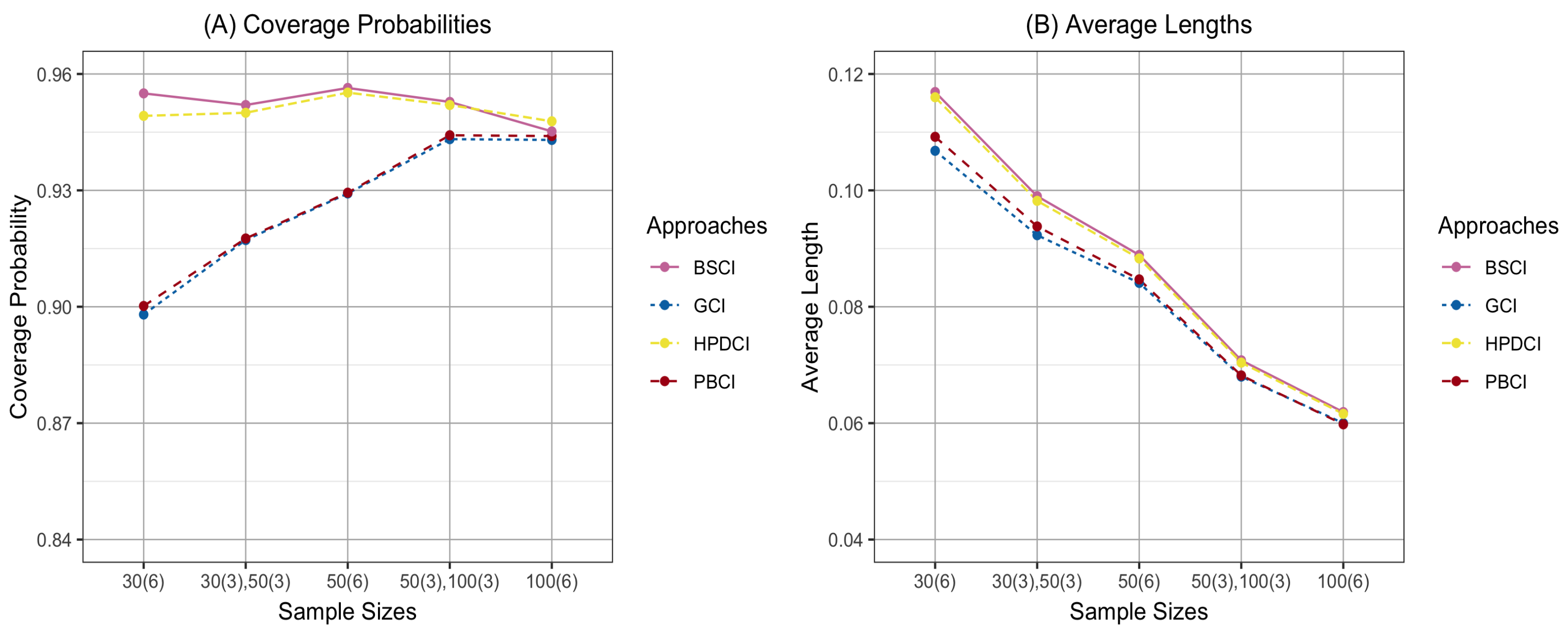
Table 1 and Table 2, together with Figure 1 and Figure 2, indicate that under small-sample conditions, the GCI and parametric bootstrap approaches often failed to attain the nominal level of 0.95, whereas the Bayesian and HPD approaches achieved more reliable coverage but with longer intervals. As the sample size increased, however, all approaches converged toward the 0.95 target and produced shorter intervals, leading to greater precision.
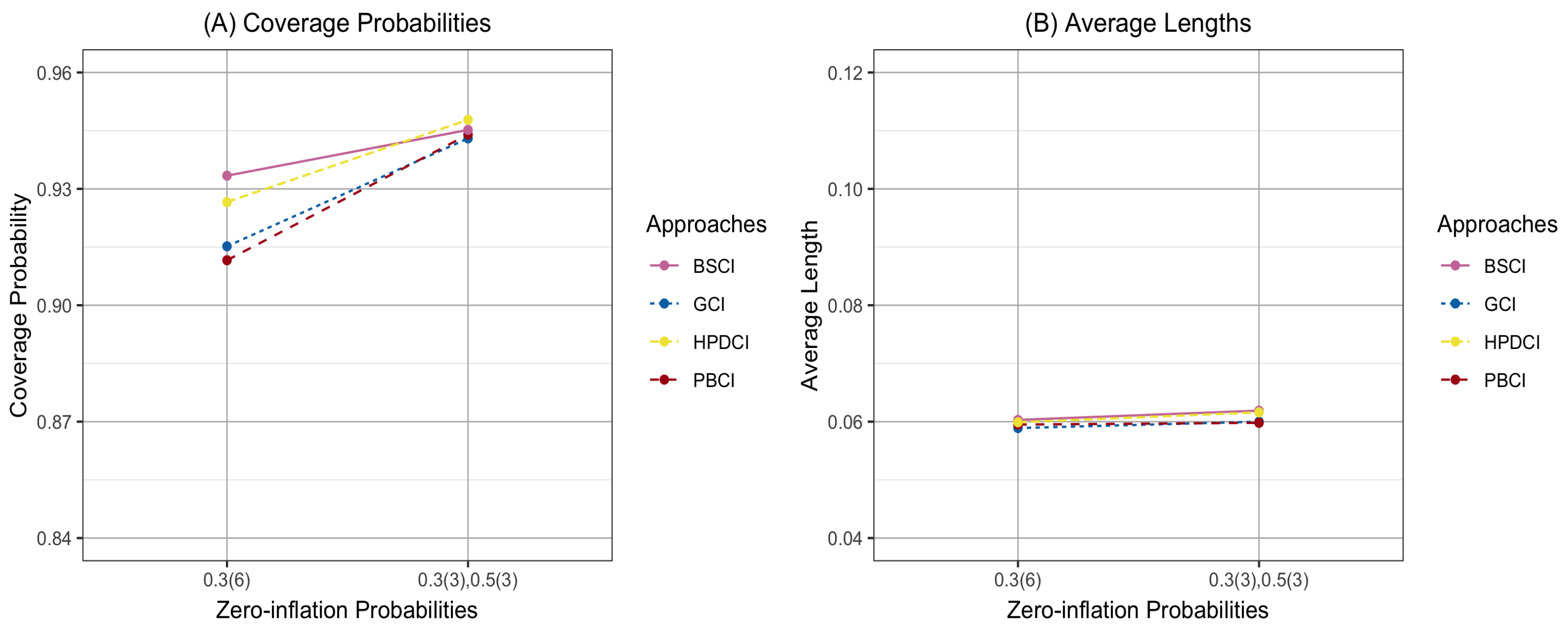
Table 1 and Table 2, supported by Figure 3 and Figure 4, further reveal that both CPs and ALs increased with higher zero-inflation probabilities. This effect was most evident for the GCI and parametric bootstrap intervals, which showed marked under-coverage in small samples. In contrast, Bayesian and HPD intervals remained more robust, maintaining coverage close to 95% even under high zero inflation. With larger samples, the negative influence of zero inflation diminished and interval precision improved.
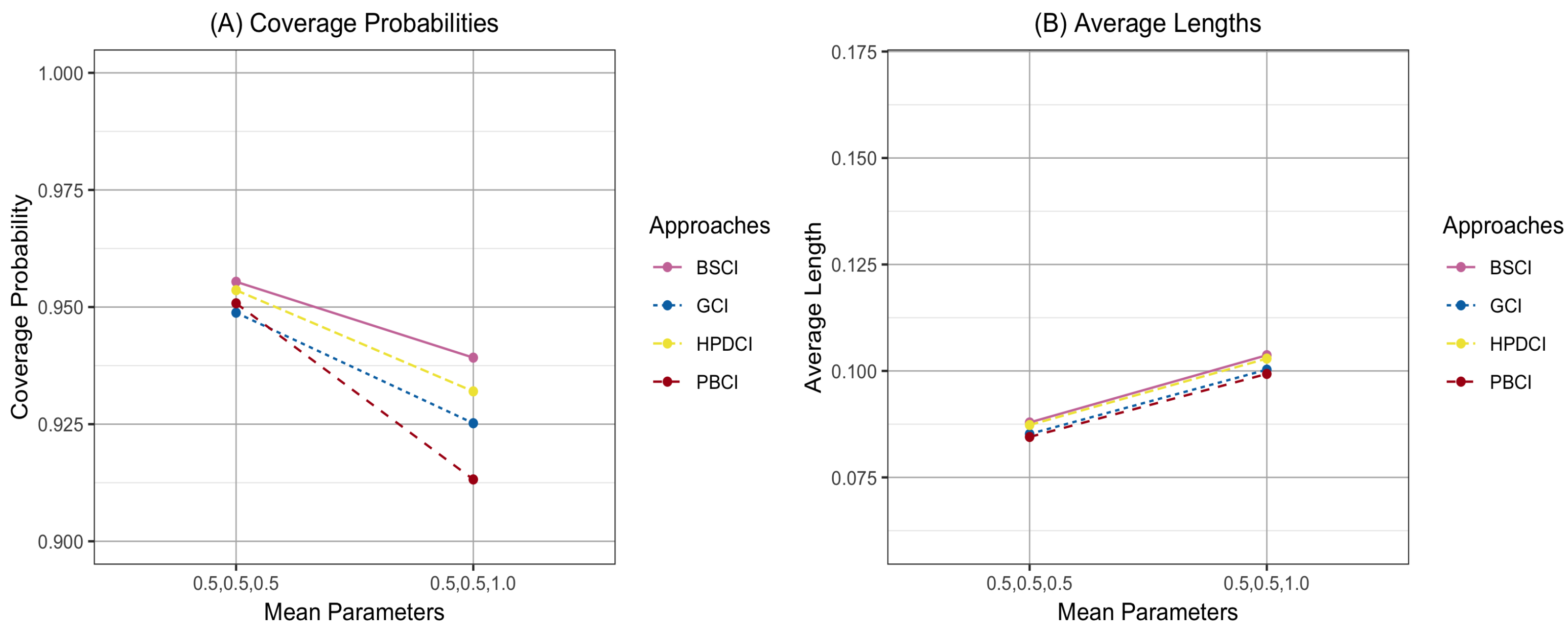
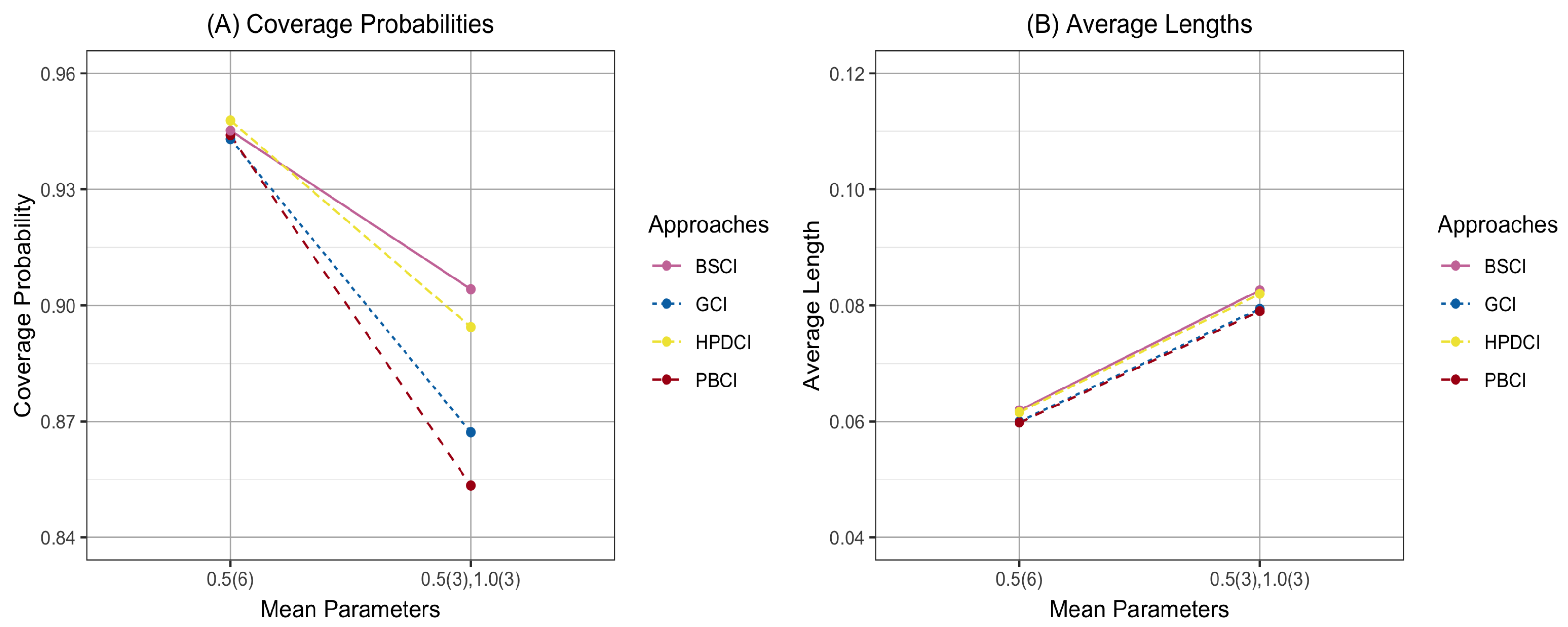
Similarly, Table 1 and Table 2, along with Figure 5 and Figure 6, demonstrate that CPs tended to fall below 0.95 as the mean increased, while ALs grew larger. Smaller mean parameters produced more skewed distributions, leading to reduced coverage for the GCI and parametric bootstrap intervals, particularly in small samples. Larger or mixed means, however, improved coverage across all approaches, with Bayesian and HPD intervals consistently providing accurate results. In the six-sample cases, the effect was more pronounced, as unequal means further accentuated the differences among methods.
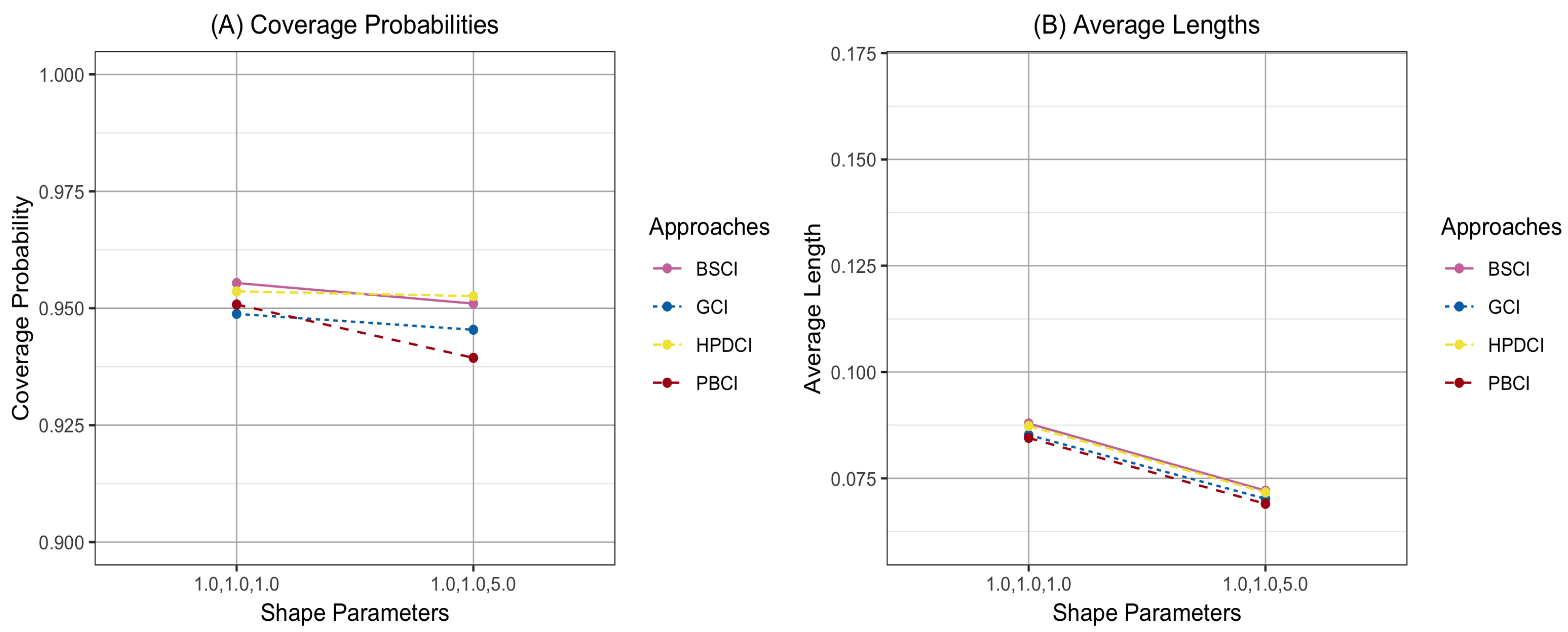
Finally, Table 1 and Table 2, together with Figure 7 and Figure 8, show that both CPs and ALs declined as the shape parameters increased. Small shape values, which introduced higher variance, produced wider intervals and lower CPs for the GCI and parametric bootstrap approaches, whereas the Bayesian and HPD approaches remained stable across different shape settings.
For the three-sample cases, Bayesian and HPD intervals consistently achieved coverage closest to 95% across all parameter configurations, with the HPD intervals often yielding slightly shorter lengths. The GCI and parametric bootstrap intervals, by contrast, tended to underperform in skewed or small-sample situations. In the six-sample cases, similar trends were observed, although the under-coverage of GCI and parametric bootstrap approaches was even more pronounced in highly skewed scenarios. The Bayesian and HPD intervals maintained greater accuracy, albeit with somewhat longer average lengths in certain settings.

5. An Empirical Application

Traffic accidents remain a major global health challenge, ranking among the leading causes of injuries and premature deaths worldwide. Beyond their devastating impact on human life, they also impose heavy economic costs on individuals, households, and governments, including healthcare expenses, productivity losses, and the long-term management of disabilities. The factors contributing to traffic accidents are diverse, encompassing human behavior, environmental conditions, and mechanical issues. Risky driving practices—such as excessive speed, alcohol use, and driver distraction—are among the primary causes, while inadequate infrastructure, unsafe road conditions, and weak law enforcement further intensify the problem. Effectively addressing this complex issue requires a multidimensional approach that combines stricter regulations, educational campaigns, infrastructure improvements, and well-coordinated emergency medical services. Gaining a deeper understanding of the patterns and underlying factors of traffic accidents is therefore vital for developing evidence-based strategies aimed at lowering accident rates and minimizing their impacts.
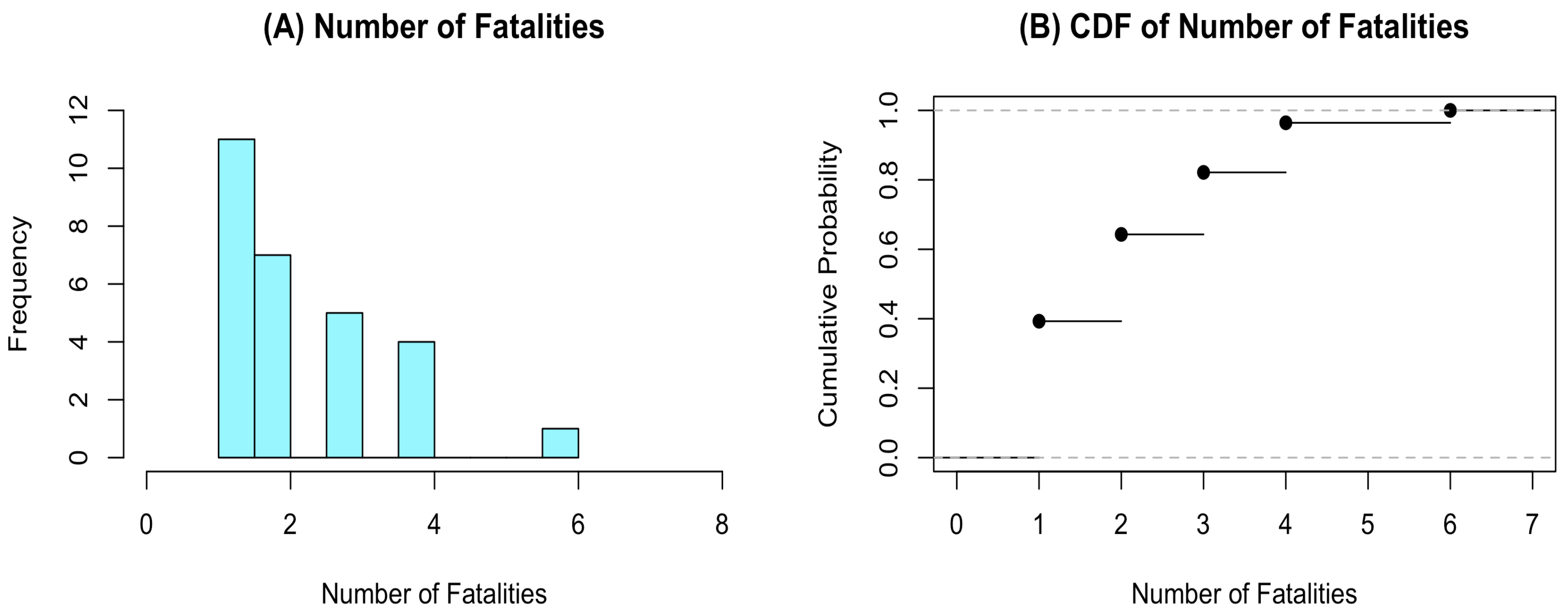
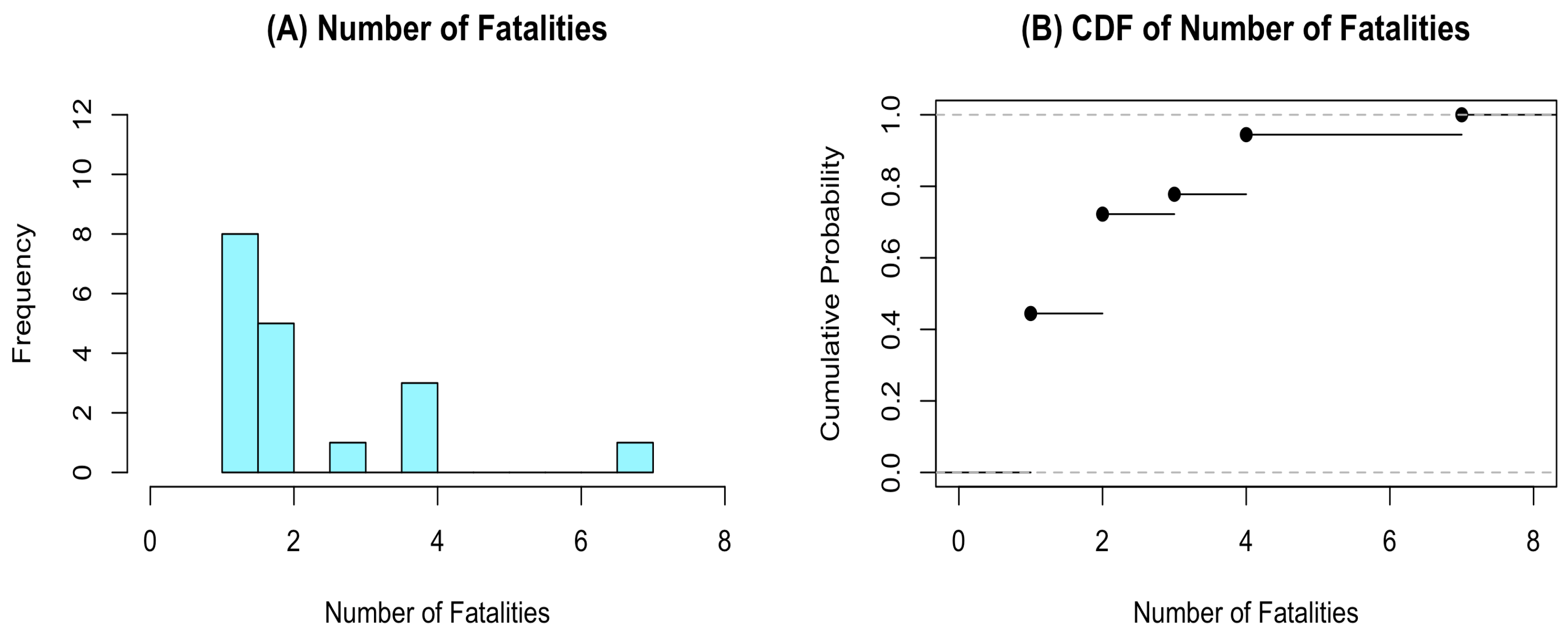
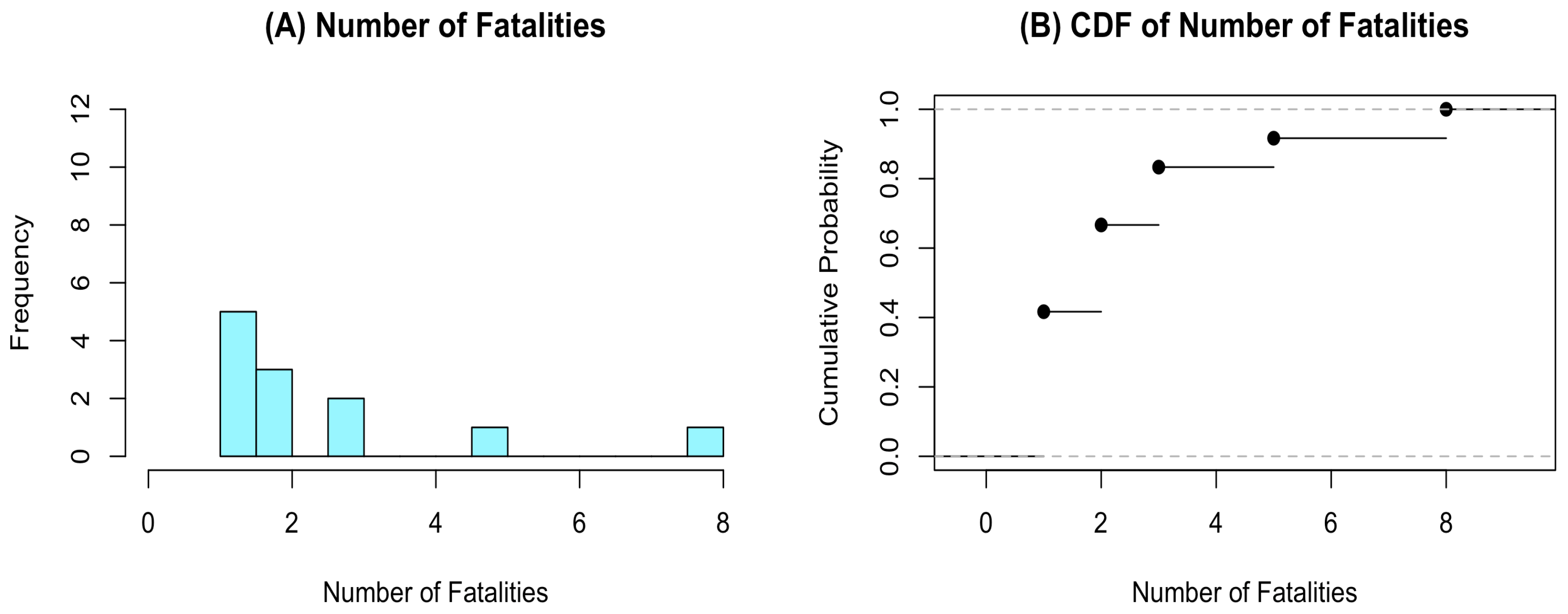
The present study utilizes casualty data from traffic accidents reported by the Road Accident Victims Protection Company Limited and published on the Thai RSC website. The analysis focuses on the number of fatalities from road accidents in April 2025 across three regions of Thailand: 50 districts in Bangkok, 33 districts in Nakhon Ratchasima province, and 19 districts in Chiang Rai province, as presented in Table 3. Figure 9, Figure 10 and Figure 11 show that the distributions of non-zero road accident fatalities in April 2025 for Bangkok, Nakhon Ratchasima, and Chiang Rai provinces are right-skewed. As presented in Table 4, the inverse Gaussian distribution yields the lowest Akaike information criterion (AIC) values. Thus, the non-zero fatalities from road accidents in these provinces are best modeled by an inverse Gaussian distribution. Since the data also include zero observations, the overall distribution of road accident fatalities is appropriately modeled using a ZIIG distribution.
Table 5 presents the descriptive statistics of the number of fatalities in Bangkok, Nakhon Ratchasima, and Chiang Rai provinces of Thailand. The common mean of fatalities across these provinces is 1.2793. As shown in Table 6, the 95% confidence intervals from all approaches for the common mean successfully cover the true common mean. Among these approaches, the parametric bootstrap confidence interval exhibits the shortest length, consistent with the simulation results reported in the previous section. However, unlike the simulation, which used 5000 repetitions, this analysis is based on a single application. In the simulation, the CPs of the parametric bootstrap interval fell below the nominal level of 0.95, indicating that it is not recommended for constructing 95% confidence intervals for the common mean of fatalities in these provinces.
In contrast, the HPD interval has a shorter length compared to the GCI and Bayesian credible intervals. Furthermore, simulation results show that the CPs of the HPD interval exceed the nominal level of 0.95. Therefore, the HPD interval is recommended for constructing 95% confidence intervals for the common mean of fatalities in Bangkok, Nakhon Ratchasima, and Chiang Rai provinces.
Although the empirical datasets analyzed in this study are of relatively small sizes, the proposed estimation framework remains highly appropriate for such applications. The ZIIG model provides a flexible structure that effectively captures both zero inflation and pronounced skewness—features commonly encountered in short or limited time series data. Furthermore, the employed estimation procedures, particularly the GCI and Bayesian approaches, have demonstrated strong stability and reliability even under small-sample conditions. Simulation results presented in Section 4, including cases with sample sizes of (30, 30, 30) and (50, 50, 50), confirm that these approaches yield satisfactory CPs and reasonable ALs. Taken together, these findings provide clear justification for applying the proposed approach to empirical datasets of small length, such as the regional traffic fatality series examined in this work.

6. Discussion

The simulation results provide several insights into the performance of the four interval estimation approaches under varying conditions. Table 1 and Table 2, together with Figure 1 and Figure 2, demonstrate that in small-sample settings, the GCI and parametric bootstrap approaches frequently failed to attain the nominal level of 0.95. By contrast, the Bayesian and HPD intervals offered more reliable coverage, albeit at the cost of longer interval lengths. As sample sizes increased, however, all approaches converged toward the nominal level, producing narrower intervals and thereby improving precision.
The influence of zero inflation is illustrated in Table 1 and Table 2, supported by Figure 3 and Figure 4. Both CPs and ALs increased under higher zero-inflation probabilities. This effect was most pronounced for the GCI and parametric bootstrap intervals, which exhibited substantial under-coverage in small samples. In contrast, the Bayesian and HPD approaches proved more robust, consistently maintaining coverage close to 95% even in the presence of high zero inflation. With larger samples, the adverse impact of zero inflation diminished, and interval precision improved across all approaches.
A related trend emerged when examining the effect of the mean parameter (Table 1 and Table 2; Figure 5 and Figure 6). As the mean increased, CPs tended to fall below 0.95, while ALs became larger. Smaller means, associated with more skewed distributions, reduced the performance of GCI and parametric bootstrap intervals in particular, especially for small samples. Larger or heterogeneous means improved coverage across all approaches, with Bayesian and HPD intervals consistently providing the most accurate results. In six-sample scenarios, these effects were more pronounced, as unequal means accentuated differences among the approaches.
Table 1 and Table 2, in conjunction with Figure 7 and Figure 8, further show that both CPs and ALs decreased as the shape parameters increased. Smaller shape values, which induce greater variance, led to wider intervals and lower coverage for the GCI and parametric bootstrap approaches. By contrast, the Bayesian and HPD intervals remained stable across shape settings, highlighting their robustness to changes in distributional variability.
Taken together, the findings suggest clear performance differences among the four approaches. For the three-sample cases, Bayesian and HPD intervals consistently achieved coverage closest to 95% across all parameter configurations, with HPD intervals often producing slightly shorter lengths. The GCI and parametric bootstrap intervals, on the other hand, tended to underperform in small-sample or highly skewed conditions. For the six-sample cases, similar trends were observed, though the under-coverage of GCI and parametric bootstrap approaches was even more pronounced in settings with high skewness. Bayesian and HPD intervals retained greater accuracy overall, although this robustness was sometimes accompanied by longer average lengths.

7. Conclusions

This study investigated the performance of four interval estimation approaches—the GCI, parametric bootstrap, Bayesian, and HPD—for estimating the common mean of ZIIG distributions under varying parameter settings and sample sizes. The findings highlighted clear differences in both accuracy and reliability across the approaches.
In small-sample situations, the GCI and parametric bootstrap approaches frequently exhibited under-coverage, particularly when distributions were highly skewed or contained substantial zero inflation. By contrast, the Bayesian and HPD intervals achieved coverage levels closer to the nominal 95%, though this often came at the cost of longer interval lengths. As sample sizes increased, however, all approaches converged toward the nominal level and produced narrower intervals, thereby improving precision.
Across variations in zero inflation, mean parameters, and shape parameters, the Bayesian and HPD approaches consistently outperformed the GCI and parametric bootstrap approaches, demonstrating greater robustness across scenarios. The HPD approach, in particular, often combined accurate coverage with slightly shorter intervals, underscoring its practical value for both small- and large-sample contexts.
Overall, the results suggest that while the GCI and parametric bootstrap approaches may still be suitable for large samples with limited skewness, the Bayesian and HPD approaches deliver more dependable performance across a wider range of conditions. These insights provide practical guidance for researchers and practitioners in selecting effective interval estimation strategies for ZIIG models.

Author Contributions

Conceptualization, S.-A.N. and W.T.; methodology, S.-A.N. and W.T.; software, W.T.; validation, S.-A.N. and S.N.; formal analysis, S.-A.N. and W.T.; investigation, S.N.; resources, W.T.; data curation, W.T.; writing—original draft preparation, W.T.; writing—review and editing, S.-A.N. and W.T.; visualization, W.T.; supervision, S.-A.N.; project administration, S.-A.N. and S.N.; funding acquisition, S.-A.N. and S.N. All authors have read and agreed to the published version of the manuscript.

Funding

This research budget was allocated by National Science, Research, and Innovation Fund (NSRF) and King Mongkut’s University of Technology North Bangkok: KMUTNB- FF-68-B-43.

Data Availability Statement

Data on the number of fatalities from road accidents were obtained from the Road Accident Victims Protection Company Limited and are available on the Thai RSC website at https://www.thairsc.com/ (accessed on 9 September 2025).

Conflicts of Interest

The authors declare no conflict of interest.

Appendix A. Variance Approximation of the ZIIZ Mean Estimator Using the Delta Method

Let X = X 1 , X 2 , , X n be a random variable that follows a ZIIG distribution. This variable comprises the count of zero outcomes ( n 0 ) and the count of non-zero outcomes ( n 1 ). The expected value (mean) of X is denoted by θ = 1 τ μ . An estimator for θ is represented as θ ^ = 1 τ ^ μ ^ . The variance of θ ^ is expressed as
V a r θ ^ = μ 2 τ ( 1 τ ) n 1 + ( 1 τ ) 2 μ 3 λ n 1 .
To approximate the variance of θ ^ , the delta method is applied. This method estimates the variance of a function involving one or more parameters. A transformation function g ( τ , μ ) is defined as
θ = g ( τ , μ ) = ( 1 τ ) μ .
Applying the delta method (Casella and Berger [25]), the approximate variance of θ ^ is given by
V a r θ ^ = V a r g ^ τ , μ g τ , μ T C o v τ ^ , μ ^ g τ , μ ,
where g τ , μ = g τ , g μ = ( μ , 1 τ ) is the gradient (vector of partial derivatives) of the transformation function g τ , μ evaluated at τ , μ .
To obtain the covariance matrix of τ ^ , μ ^ , the Fisher information matrix is required. In the case of the Fisher information related to the zero-inflation parameter, the zero-inflated component is modeled using a Bernoulli distribution. The zero-inflated model uses a Bernoulli distribution to distinguish between two sources of zeros: structural zeros and zeros from the standard count process (e.g., Poisson or Negative Binomial). The Bernoulli component models the probability that an observation is a structural zero, allowing the model to more accurately capture excess zeros in the data. The Fisher information for this part is defined as
I τ = 1 τ ( 1 τ ) .
The variance for τ ^ is given by
V a r τ ^ = τ ( 1 τ ) n 1 .
For the Fisher information corresponding to the parameter μ , the standard inverse Gaussian distribution provides the Fisher information as
I μ = λ μ 3 .
The variance for μ ^ is calculated as
V a r μ ^ μ 3 λ n 1 .
To determine the covariance between τ ^ and μ ^ , if these two parameters are estimated independently, then their covariance is zero ( C o v τ ^ , μ ^ = 0 ). As a result, the asymptotic covariance matrix takes the form
C o v τ ^ , μ ^ = τ ( 1 τ ) n 1 0 0 μ 3 λ n 1 .
By applying the delta method with the transformation function g τ , μ , the variance is approximated as
V a r θ ^ = μ 1 τ τ ( 1 τ ) n 1 0 0 μ 3 λ n 1 μ 1 τ = μ τ 1 τ n 1 1 τ μ 3 λ n 1 μ 1 τ = μ 2 τ 1 τ n 1 + 1 τ 2 μ 3 λ n 1 = μ 2 τ 1 τ n 1 + 1 τ 2 μ 3 λ n 1 .
Thus, the variance of the mean for the ZIIG distribution is expressed as
V a r θ ^ = μ 2 τ 1 τ n 1 + 1 τ 2 μ 3 λ n 1 .
In this expression, the first term μ 2 τ 1 τ n 1 captures the uncertainty arising from the zero-inflation component, while the second term 1 τ 2 μ 3 λ n 1 reflects the variability due to the inverse Gaussian part of the model.

Appendix B. Derivation of the Posterior Distribution for the ZIIG Model

Bayes’ Theorem forms the foundation of this approach, defining the posterior distribution as the product of the prior distribution and the likelihood of the observed data. This structure enables the integration of previous knowledge with current observations in a coherent and principled way, making the Bayesian method particularly useful for parameter estimation, forecasting, and hypothesis evaluation, especially in complex models or when dealing with limited data.
A major advantage of the Bayesian framework is its capacity to explicitly handle uncertainty and incorporate expert knowledge. Instead of providing only point estimates, it generates full probability distributions for parameters, allowing for a more informative and transparent understanding of the results.
The prior density function f θ i must be specified. This prior represents the initial beliefs about the parameters before observing the data. In the Bayesian framework for the ZIIG model, different priors are assigned to different parameters based on their roles and characteristics. Specifically, a uniform prior is used for the mean parameter θ ^ i . B S to reflect non-informative prior knowledge, ensuring that no specific value is favored a priori within a specified range. For the shape parameter μ ^ i . B S , a gamma prior is chosen due to its flexibility in modeling positive continuous parameters and its conjugacy with many likelihoods, which facilitates posterior computation. The zero-inflation parameter τ ^ i . B S , which lies between 0 and 1, is assigned a beta prior, as the beta distribution is naturally defined on the unit interval and can capture a wide range of prior beliefs about the probability of excess zeros.
The hyperparameters of these priors (e.g., the shape and rate for the gamma prior, or the α and β parameters of the beta prior) are either chosen based on empirical data, expert elicitation, or set to values that reflect vague or weakly informative priors when prior knowledge is limited. These choices are crucial, as they influence the shape of the posterior distribution and, consequently, the parameter estimates. Incorporating these carefully selected priors within the Bayesian framework allows for coherent inference, effective posterior sampling via MCMC methods, and reliable estimation of the model parameters, particularly τ ^ i . B S , in the presence of zero inflation.
The likelihood function corresponding to the ZIIG distribution is given by
L θ i | X i j τ n i ( 0 ) 1 τ i n i ( 1 ) λ i n i ( 1 ) / 2 exp λ i 2 μ i 2 j = 1 n i X i j 2 n i ( 1 ) μ i + j = 1 n i 1 X i j μ i 2 .
The posterior distribution of the parameters is obtained by combining the prior distribution with the likelihood function derived from the ZIIG model. According to Bayes’ Theorem, the posterior is proportional to the product of the prior and the likelihood:
f θ i | X i j f θ i L θ i | X i j .
This distribution represents the updated beliefs about the parameters θ i = θ ^ i . B S , μ ^ i . B S , τ ^ i . B S after observing the data X i j . It captures both the information provided by the observed data and the assumptions or prior knowledge encoded in the prior distributions. The posterior distribution provides not just point estimates but full probability distributions for each parameter, allowing for uncertainty quantification through credible intervals and probabilistic interpretation.
However, due to the analytical complexity of the ZIIG model, the posterior distribution cannot be obtained in closed form. To address this, Markov Chain Monte Carlo (MCMC) methods—particularly the Metropolis-within-Gibbs algorithm—are employed to generate samples from the posterior. These samples allow estimation of posterior summaries such as means, medians, variances, and credible intervals. Incorporating these carefully selected priors within the Bayesian framework thus enables coherent inference, effective posterior sampling, and reliable estimation of the model parameters, especially the zero-inflation parameter τ ^ i . B S , which is crucial in capturing the excess zeros in the data.

References

  1. Krishnamoorthy, K.; Tian, L. Inferences on the difference and ratio of the means of two inverse Gaussian distributions. J. Stat. Plan. Inference 2008, 138, 2082–2089. [Google Scholar] [CrossRef]
  2. Punzo, A. A new look at the inverse Gaussian distribution with applications to insurance and economic data. J. Appl. Stat. 2019, 46, 1260–1287. [Google Scholar] [CrossRef]
  3. Gelman, A.; Hill, J. Data Analysis Using Regression and Multilevel/Hierarchical Models; Cambridge University Press: New York, NY, USA, 2007. [Google Scholar]
  4. Borenstein, M.; Hedges, L.V.; Higgins, J.P.T.; Rothstein, H.R. Introduction to Meta-Analysis; John Wiley & Sons, Ltd.: Chichester, UK, 2009. [Google Scholar]
  5. Katahira, K. How hierarchical models improve point estimates of individual-level parameters. J. Math. Psychol. 2016, 73, 37–58. [Google Scholar] [CrossRef]
  6. Slud, E.V.; Vonta, I.; Kagan, A.M. Combining estimators of a common parameter across samples. Stat. Theory Relat. Fields 2018, 2, 158–171. [Google Scholar] [CrossRef]
  7. Ye, R.D.; Ma, T.F.; Wang, S.G. Inferences on the common mean of several inverse Gaussian populations. Comput. Stat. Data Anal. 2010, 54, 906–915. [Google Scholar] [CrossRef]
  8. Bera, S.; Jana, N. On estimating common mean of several inverse Gaussian distributions. Metrika 2022, 85, 115–139. [Google Scholar] [CrossRef]
  9. Jana, N.; Gautam, M. Confidence intervals of difference and ratio of means for zero-adjusted inverse Gaussian distributions. Commun. Stat. Simul. Comput. 2022, 53, 3302–3326. [Google Scholar] [CrossRef]
  10. Khumpasee, W.; Niwitpong, S.A.; Niwitpong, S. Confidence intervals for the coefficient of variation in delta-inverse Gaussian distributions. Symmetry 2024, 16, 1488. [Google Scholar] [CrossRef]
  11. Niwitpong, S.A.; Khumpasee, W.; Niwitpong, S. Confidence intervals for the variance of delta-inverse Gaussian distribution with application to traffic mortality count. J. Phys. Conf. Ser. 2025, 3041, 012009. [Google Scholar] [CrossRef]
  12. Weerahandi, S. Generalized confidence intervals. J. Am. Stat. Assoc. 1993, 88, 899–905. [Google Scholar] [CrossRef]
  13. Krishnamoorthy, K.; Lu, Y. Inference on the common means of several normal populations based on the generalized variable method. Biometrics 2003, 59, 237–247. [Google Scholar] [CrossRef]
  14. Tian, L. Inferences on the common coefficient of variation. Stat. Med. 2005, 24, 2213–2220. [Google Scholar] [CrossRef]
  15. Chen, Y.H.; Zhou, X.H. Generalized Confidence Intervals for the Ratio or Difference of Two Means for Lognormal Populations with Zeros; UW Biostatistics Working Paper Series; Working Paper 296; Elsevier: Amsterdam, The Netherlands, 2006; pp. 1–26. [Google Scholar]
  16. Tian, L.; Wu, J. Inferences on the common mean of several log-normal populations: The generalized variable approach. Biometrical J. 2007, 49, 944–951. [Google Scholar] [CrossRef]
  17. Padgett, W.J.; Tomlinson, M.A. Lower confidence bounds for percentiles of Weibull and Birnbaum-Saunders distributions. J. Stat. Comput. Simul. 2003, 73, 429–443. [Google Scholar] [CrossRef]
  18. Altunkaynak, B.; Gamgam, H. Bootstrap confidence intervals for the coefficient of quartile variation. Commun. Stat. Simul. Comput. 2019, 48, 2138–2146. [Google Scholar] [CrossRef]
  19. Zhang, G. A parametric bootstrap approach for one-way ANOVA under unequal variances with unbalanced data. Commun. Stat. Simul. Comput. 2015, 44, 827–832. [Google Scholar] [CrossRef]
  20. Aizpurua, J.I.; Stewart, B.G.; McArthur, S.D.J.; Penalba, M.; Barrenetxea, M.; Muxika, E.; Ringwood, J.V. Probabilistic forecasting informed failure prognostics framework for improved RUL prediction under uncertainty: A transformer case study. Reliab. Eng. Syst. Saf. 2022, 226, 108676. [Google Scholar] [CrossRef]
  21. Harvey, J.; van der Merwe, A.J. Bayesian confidence intervals for means and variances of lognormal and bivariate lognormal distributions. J. Stat. Plan. Inference 2012, 142, 1294–1309. [Google Scholar] [CrossRef]
  22. Rao, K.A.; D’Cunha, J.G. Bayesian inference for median of the lognormal distribution. J. Mod. Appl. Stat. Methods 2016, 15, 526–535. [Google Scholar] [CrossRef]
  23. Ma, Z.; Chen, G. Bayesian methods for dealing with missing data problems. J. Korean Stat. Soc. 2018, 47, 297–313. [Google Scholar] [CrossRef]
  24. Wu, W.H.; Hsieh, H.N. Generalized confidence interval estimation for the mean of delta-lognormal distribution: An application to New Zealand trawl survey data. J. Appl. Stat. 2014, 41, 1471–1485. [Google Scholar] [CrossRef]
  25. Casella, G.; Berger, R.L. Statistical Inference; Duxbury: Bolinas, CA, USA, 2002. [Google Scholar]
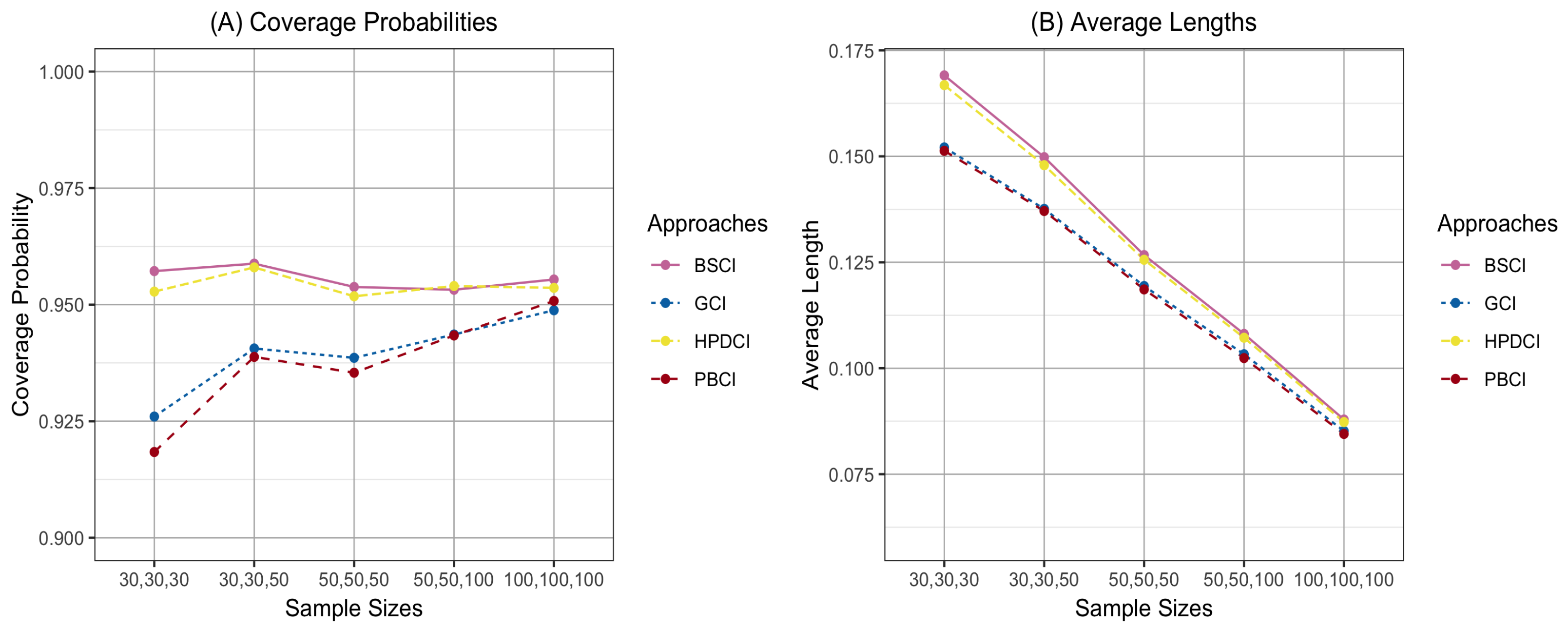
Figure 1. Comparison of the CPs (A) and ALs (B) of the four approaches across different sample sizes when ( τ 1 , τ 2 , τ 3 ) = (0.3,0.3,0.5), ( μ 1 , μ 2 , μ 3 ) = (0.5,0.5,0.5), and ( λ 1 , λ 2 , λ 3 ) = (1.0,1.0,1.0).
Symmetry 17 01944 g001
Figure 2. Comparison of the CPs (A) and ALs (B) of the four approaches across different sample sizes when ( τ 1 , τ 2 , τ 3 , τ 4 , τ 5 , τ 6 ) = (0.3,0.3,0.3,0.5,0.5,0.5), ( μ 1 , μ 2 , μ 3 , μ 4 , μ 5 , μ 6 ) = (0.5,0.5,0.5, 0.5,0.5,0.5), and ( λ 1 , λ 2 , λ 3 , λ 4 , λ 5 , λ 6 ) = (1.0,1.0,1.0,1.0,1.0,1.0).
Symmetry 17 01944 g002
Figure 3. Comparison of the CPs (A) and ALs (B) of the four approaches across different zero-inflation probabilities when ( n 1 , n 2 , n 3 ) = (100,100,100), ( μ 1 , μ 2 , μ 3 ) = (0.5,0.5,0.5), and ( λ 1 , λ 2 , λ 3 ) = (1.0,1.0,1.0).
Symmetry 17 01944 g003
Figure 4. Comparison of the CPs (A) and ALs (B) of the four approaches across different zero-inflation probabilities when ( n 1 , n 2 , n 3 , n 4 , n 5 , n 6 ) = (100,100,100,100,100,100), ( μ 1 , μ 2 , μ 3 , μ 4 , μ 5 , μ 6 ) = (0.5,0.5,0.5,0.5,0.5,0.5), and ( λ 1 , λ 2 , λ 3 , λ 4 , λ 5 , λ 6 ) = (1.0,1.0,1.0,1.0,1.0,1.0).
Symmetry 17 01944 g004
Figure 5. Comparison of the CPs (A) and ALs (B) of the four approaches across different mean parameters when ( n 1 , n 2 , n 3 ) = (100,100,100), ( τ 1 , τ 2 , τ 3 ) = (0.3,0.3,0.5), and ( λ 1 , λ 2 , λ 3 ) = (1.0,1.0,1.0).
Symmetry 17 01944 g005
Figure 6. Comparison of the CPs (A) and ALs (B) of the four approaches across different mean parameters when ( n 1 , n 2 , n 3 , n 4 , n 5 , n 6 ) = (100,100,100,100,100,100), ( τ 1 , τ 2 , τ 3 , τ 4 , τ 5 , τ 6 ) = (0.3,0.3,0.3,0.5,0.5,0.5), and ( λ 1 , λ 2 , λ 3 , λ 4 , λ 5 , λ 6 ) = (1.0,1.0,1.0,1.0,1.0,1.0).
Symmetry 17 01944 g006
Figure 7. Comparison of the CPs (A) and ALs (B) of the four approaches across different shape parameters when ( n 1 , n 2 , n 3 ) = (100,100,100), ( τ 1 , τ 2 , τ 3 ) = (0.3,0.3,0.5), and ( μ 1 , μ 2 , μ 3 ) = (0.5,0.5,0.5).
Symmetry 17 01944 g007
Figure 8. Comparison of the CPs (A) and ALs (B) of the four approaches across different shape parameters when ( n 1 , n 2 , n 3 , n 4 , n 5 , n 6 ) = (100,100,100,100,100,100), ( τ 1 , τ 2 , τ 3 , τ 4 , τ 5 , τ 6 ) = (0.3,0.3,0.3,0.5,0.5,0.5), and ( μ 1 , μ 2 , μ 3 , μ 4 , μ 5 , μ 6 ) = (0.5,0.5,0.5,0.5,0.5,0.5).
Symmetry 17 01944 g008
Figure 9. Histogram (A) and cumulative distribution function (CDF) (B) of the number of fatalities in Bangkok.
Symmetry 17 01944 g009
Figure 10. Histogram (A) and CDF (B) of the number of fatalities in Nakhon Ratchasima province.
Symmetry 17 01944 g010
Figure 11. Histogram (A) and CDF (B) of the number of fatalities in Chiang Rai province.
Symmetry 17 01944 g011
Table 1. The CPs and ALs of 95% confidence intervals for the common mean of delta-inverse Gaussian distributions: 3 sample cases.
( n 1 , n 2 , n 3 ) ( τ 1 , τ 2 , τ 3 ) ( μ 1 , μ 2 , μ 3 ) ( λ 1 , λ 2 , λ 3 ) CP (AL)
CI GCI CI PB CI BS CI HPD
30,30,300.3,0.3,0.30.5,0.5,0.51.0,1.0,1.00.90860.89960.94000.9274
(0.1496)(0.1507)(0.1638)(0.1616)
0.5,0.5,0.51.0,1.0,5.00.93160.93780.95580.9474
(0.1314)(0.1353)(0.1381)(0.1371)
0.5,0.5,1.01.0,1.0,1.00.91480.89820.94820.9346
(0.1872)(0.1823)(0.2118)(0.2074)
0.5,0.5,1.01.0,1.0,5.00.91680.90780.93860.9316
(0.2041)(0.2044)(0.2236)(0.2192)
0.3,0.3,0.50.5,0.5,0.51.0,1.0,1.00.92600.91840.95720.9528
(0.1521)(0.1513)(0.1691)(0.1668)
0.5,0.5,0.51.0,1.0,5.00.94560.94340.96720.9662
(0.1284)(0.1281)(0.1391)(0.1380)
0.5,0.5,1.01.0,1.0,1.00.89760.87140.94200.9276
(0.1774)(0.1761)(0.2007)(0.1968)
0.5,0.5,1.01.0,1.0,5.00.91520.90240.94920.9356
(0.1793)(0.1783)(0.1986)(0.1952)
30,30,500.3,0.3,0.30.5,0.5,0.51.0,1.0,1.00.91120.89620.94000.9304
(0.1356)(0.1365)(0.1457)(0.1440)
0.5,0.5,0.51.0,1.0,5.00.92740.93200.94680.9406
(0.1146)(0.1179)(0.1188)(0.1181)
0.5,0.5,1.01.0,1.0,1.00.91020.88760.94420.9322
(0.1903)(0.1842)(0.2166)(0.2123)
0.5,0.5,1.01.0,1.0,5.00.90640.88800.93660.9244
(0.2046)(0.2034)(0.2252)(0.2214)
0.3,0.3,0.50.5,0.5,0.51.0,1.0,1.00.94060.93880.95880.9580
(0.1376)(0.1371)(0.1498)(0.1479)
0.5,0.5,0.51.0,1.0,5.00.95020.94820.96880.9680
(0.1116)(0.1120)(0.1184)(0.1176)
0.5,0.5,1.01.0,1.0,1.00.88880.86160.93220.9218
(0.1736)(0.1710)(0.1957)(0.1921)
0.5,0.5,1.01.0,1.0,5.00.89420.87460.93280.9178
(0.1745)(0.1738)(0.1919)(0.1892)
50,50,500.3,0.3,0.30.5,0.5,0.51.0,1.0,1.00.92180.91320.94220.9330
(0.1171)(0.1176)(0.1233)(0.1221)
0.5,0.5,0.51.0,1.0,5.00.93680.93920.95060.9460
(0.1027)(0.1045)(0.1055)(0.1049)
0.5,0.5,1.01.0,1.0,1.00.93740.92480.95640.9490
(0.1489)(0.1456)(0.1597)(0.1577)
0.5,0.5,1.01.0,1.0,5.00.92620.92020.94220.9322
(0.1604)(0.1608)(0.1688)(0.1666)
0.3,0.3,0.50.5,0.5,0.51.0,1.0,1.00.93860.93540.95380.9518
(0.1194)(0.1186)(0.1267)(0.1256)
0.5,0.5,0.51.0,1.0,5.00.95000.94860.96580.9638
(0.0993)(0.0985)(0.1043)(0.1037)
0.5,0.5,1.01.0,1.0,1.00.91600.89480.94240.9288
(0.1400)(0.1383)(0.1499)(0.1481)
0.5,0.5,1.01.0,1.0,5.00.91920.90640.94320.9318
(0.1410)(0.1406)(0.1491)(0.1475)
50,50,1000.3,0.3,0.30.5,0.5,0.51.0,1.0,1.00.93160.92420.94760.9410
(0.1020)(0.1023)(0.1059)(0.1051)
0.5,0.5,0.51.0,1.0,5.00.94260.94400.95220.9476
(0.0842)(0.0856)(0.0858)(0.0854)
0.5,0.5,1.01.0,1.0,1.00.92880.90760.94920.9416
(0.1524)(0.1478)(0.1644)(0.1623)
0.5,0.5,1.01.0,1.0,5.00.92260.91100.94200.9332
(0.1627)(0.1626)(0.1726)(0.1707)
0.3,0.3,0.50.5,0.5,0.51.0,1.0,1.00.94360.94340.95320.9540
(0.1033)(0.1024)(0.1081)(0.1072)
0.5,0.5,0.51.0,1.0,5.00.94980.94480.96100.9606
(0.0814)(0.0808)(0.0842)(0.0838)
0.5,0.5,1.01.0,1.0,1.00.91320.89100.94020.9302
(0.1372)(0.1352)(0.1466)(0.1450)
0.5,0.5,1.01.0,1.0,5.00.91220.89180.93660.9278
(0.1364)(0.1361)(0.1437)(0.1424)
100,100,1000.3,0.3,0.30.5,0.5,0.51.0,1.0,1.00.93880.93320.94840.9458
(0.0837)(0.0838)(0.0858)(0.0852)
0.5,0.5,0.51.0,1.0,5.00.94900.94720.95360.9510
(0.0729)(0.0735)(0.0739)(0.0735)
0.5,0.5,1.01.0,1.0,1.00.94560.93320.95240.9478
(0.1071)(0.1051)(0.1112)(0.1103)
0.5,0.5,1.01.0,1.0,5.00.93940.93420.94680.9420
(0.1150)(0.1151)(0.1184)(0.1173)
0.3,0.3,0.50.5,0.5,0.51.0,1.0,1.00.94880.95080.95540.9536
(0.0852)(0.0845)(0.0879)(0.0873)
0.5,0.5,0.51.0,1.0,5.00.94540.93940.95100.9526
(0.0702)(0.0690)(0.0721)(0.0717)
0.5,0.5,1.01.0,1.0,1.00.92520.91320.93920.9320
(0.1003)(0.0993)(0.1037)(0.1029)
0.5,0.5,1.01.0,1.0,5.00.92320.91560.93460.9264
(0.1008)(0.1004)(0.1036)(0.1028)
Table 2. The CPs and ALs of 95% confidence intervals for the common mean of delta-inverse Gaussian distributions: 6 sample cases.
( n 1 , n 2 , n 3 , n 4 , n 5 , n 6 ) ( τ 1 , τ 2 , τ 3 , τ 4 , τ 5 , τ 6 ) ( μ 1 , μ 2 , μ 3 , μ 4 , μ 5 , μ 6 ) ( λ 1 , λ 2 , λ 3 , λ 4 , λ 5 , λ 6 ) CP (AL)
CI GCI CI PB CI BS CI HPD
30,30,30,30,30,300.3,0.3,0.3,0.3,0.3,0.30.5,0.5,0.5,0.5,0.5,0.51.0,1.0,1.0,1.0,1.0,1.00.82740.83420.88760.8734
(0.1038)(0.1079)(0.1121)(0.1112)
0.5,0.5,0.5,0.5,0.5,0.51.0,1.0,1.0,5.0,5.0,5.00.92300.94200.92900.9230
(0.0903)(0.0957)(0.0926)(0.0921)
0.5,0.5,0.5,1.0,1.0,1.01.0,1.0,1.0,1.0,1.0,1.00.88480.86700.92920.9112
(0.1513)(0.1516)(0.1698)(0.1677)
0.5,0.5,0.5,1.0,1.0,1.01.0,1.0,1.0,5.0,5.0,5.00.90120.90100.91420.8978
(0.1679)(0.1745)(0.1803)(0.1782)
0.3,0.3,0.3,0.5,0.5,0.50.5,0.5,0.5,0.5,0.5,0.51.0,1.0,1.0,1.0,1.0,1.00.89800.90020.95500.9492
(0.1068)(0.1092)(0.1169)(0.1160)
0.5,0.5,0.5,0.5,0.5,0.51.0,1.0,1.0,5.0,5.0,5.00.95140.95120.97320.9714
(0.0881)(0.0890)(0.0933)(0.0928)
0.5,0.5,0.5,1.0,1.0,1.01.0,1.0,1.0,1.0,1.0,1.00.80340.78420.89220.8716
(0.1372)(0.1408)(0.1544)(0.1527)
0.5,0.5,0.5,1.0,1.0,1.01.0,1.0,1.0,5.0,5.0,5.00.85500.84980.90760.8898
(0.1408)(0.1442)(0.1540)(0.1525)
30,30,30,50,50,500.3,0.3,0.3,0.3,0.3,0.30.5,0.5,0.5,0.5,0.5,0.51.0,1.0,1.0,1.0,1.0,1.00.85520.85540.90020.8878
(0.0912)(0.0941)(0.0966)(0.0960)
0.5,0.5,0.5,0.5,0.5,0.51.0,1.0,1.0,5.0,5.0,5.00.93160.94460.93800.9336
(0.0753)(0.0786)(0.0767)(0.0764)
0.5,0.5,0.5,1.0,1.0,1.01.0,1.0,1.0,1.0,1.0,1.00.86840.84120.92920.9094
(0.1537)(0.1524)(0.1733)(0.1713)
0.5,0.5,0.5,1.0,1.0,1.01.0,1.0,1.0,5.0,5.0,5.00.88800.87500.91920.9034
(0.1645)(0.1700)(0.1782)(0.1766)
0.3,0.3,0.3,0.5,0.5,0.50.5,0.5,0.5,0.5,0.5,0.51.0,1.0,1.0,1.0,1.0,1.00.91720.91760.95200.9500
(0.0923)(0.0938)(0.0990)(0.0982)
0.5,0.5,0.5,0.5,0.5,0.51.0,1.0,1.0,5.0,5.0,5.00.94700.94500.96560.9638
(0.0736)(0.0745)(0.0768)(0.0764)
0.5,0.5,0.5,1.0,1.0,1.01.0,1.0,1.0,1.0,1.0,1.00.78940.76400.88320.8652
(0.1339)(0.1353)(0.1503)(0.1487)
0.5,0.5,0.5,1.0,1.0,1.01.0,1.0,1.0,5.0,5.0,5.00.83580.82620.89820.8824
(0.1349)(0.1384)(0.1464)(0.1452)
50,50,50,50,50,500.3,0.3,0.3,0.3,0.3,0.30.5,0.5,0.5,0.5,0.5,0.51.0,1.0,1.0,1.0,1.0,1.00.87640.87260.91320.9002
(0.0821)(0.0840)(0.0859)(0.0854)
0.5,0.5,0.5, 0.5,0.5,0.51.0,1.0,1.0,5.0,5.0,5.00.94320.94940.94720.9438
(0.0697)(0.0721)(0.0708)(0.0705)
0.5,0.5,0.5,1.0,1.0,1.0.0,1.0,1.0,1.0,1.0,1.00.90180.88960.93340.9204
(0.1215)(0.1203)(0.1308)(0.1296)
0.5,0.5,0.5,1.0,1.0,1.01.0,1.0,1.0,5.0,5.0,5.00.91300.91000.92300.9102
(0.1330)(0.1364)(0.1391)(0.1378)
0.3,0.3,0.3,0.5,0.5,0.50.5,0.5,0.5,0.5,0.5,0.51.0,1.0,1.0,1.0,1.0,1.00.92920.92940.95640.9552
(0.0841)(0.0847)(0.0889)(0.0883)
0.5,0.5,0.5,0.5,0.5,0.51.0,1.0,1.0,5.0,5.0,5.00.94920.94240.95980.9602
(0.0673)(0.0671)(0.0701)(0.0698)
0.5,0.5,0.5,1.0,1.0,1.01.0,1.0,1.0,1.0,1.0,1.00.83820.81880.89700.8784
(0.1095)(0.1103)(0.1177)(0.1167)
0.5,0.5,0.5,1.0,1.0,1.01.0,1.0,1.0,5.0,5.0,5.00.85880.85200.89720.8814
(0.1109)(0.1124)(0.1169)(0.1160)
50,50,50,100,100,1000.3,0.3,0.3, 0.3,0.3,0.30.5,0.5,0.5,0.5,0.5,0.51.0,1.0,1.0,1.0,1.0,1.00.90160.89780.92720.9206
(0.0677)(0.0689)(0.0699)(0.0695)
0.5,0.5,0.5,0.5,0.5,0.51.0,1.0,1.0,5.0,5.0,5.00.93340.94320.93960.9378
(0.0540)(0.0551)(0.0546)(0.0544)
0.5,0.5,0.5,1.0,1.0,1.01.0,1.0,1.0,1.0,1.0,1.00.90180.87500.94080.9306
(0.1237)(0.1216)(0.1336)(0.1325)
0.5,0.5,0.5,1.0,1.0,1.01.0,1.0,1.0,5.0,5.0,5.00.91200.89380.93600.9238
(0.1280)(0.1310)(0.1350)(0.1341)
0.3,0.3,0.3,0.5,0.5,0.50.5,0.5,0.5, 0.5,0.5,0.51.0,1.0,1.0,1.0,1.0,1.00.94320.94420.95280.9520
(0.0680)(0.0682)(0.0708)(0.0704)
0.5,0.5,0.5, 0.5,0.5,0.51.0,1.0,1.0,5.0,5.0,5.00.95080.93940.95780.9584
(0.0528)(0.0525)(0.0542)(0.0540)
0.5,0.5,0.5,1.0,1.0,1.01.0,1.0,1.0,1.0,1.0,1.00.80940.78080.88120.8654
(0.1054)(0.1054)(0.1129)(0.1121)
0.5,0.5,0.5,1.0,1.0,1.01.0,1.0,1.0,5.0,5.0,5.00.83760.81720.88400.8696
(0.1036)(0.1051)(0.1085)(0.1078)
100,100,100,100,100,1000.3,0.3,0.3, 0.3,0.3,0.30.5,0.5,0.5, 0.5,0.5,0.51.0,1.0,1.0,1.0,1.0,1.00.91520.91160.93340.9266
(0.0589)(0.0595)(0.0603)(0.0599)
0.5,0.5,0.5, 0.5,0.5,0.51.0,1.0,1.0,5.0,5.0,5.00.94020.94460.94320.9414
(0.0491)(0.0498)(0.0495)(0.0493)
0.5,0.5,0.5,1.0,1.0,1.01.0,1.0,1.0,1.0,1.0,1.00.92680.91620.94120.9342
(0.0884)(0.0872)(0.0924)(0.0917)
0.5,0.5,0.5,1.0,1.0,1.01.0,1.0,1.0,5.0,5.0,5.00.93120.93060.93660.9302
(0.0955)(0.0969)(0.0984)(0.0977)
0.3,0.3,0.3,0.5,0.5,0.50.5,0.5,0.5,0.5,0.5,0.51.0,1.0,1.0,1.0,1.0,1.00.94300.94400.94520.9478
(0.0600)(0.0598)(0.0619)(0.0616)
0.5,0.5,0.5,0.5,0.5,0.51.0,1.0,1.0,5.0,5.0,5.00.93160.91600.93440.9344
(0.0472)(0.0465)(0.0484)(0.0482)
0.5,0.5,0.5,1.0,1.0,1.01.0,1.0,1.0,1.0,1.0,1.00.86720.85340.90420.8944
(0.0794)(0.0790)(0.0826)(0.0820)
0.5,0.5,0.5,1.0,1.0,1.01.0,1.0,1.0,5.0,5.0,5.00.87320.86440.90080.8896
(0.0797)(0.0802)(0.0820)(0.0815)
Table 3. The number of fatalities from road accidents in Bangkok, Nakhon Ratchasima, and Chiang Rai provinces of Thailand.
Provinces                      Number of Fatalities
Bangkok1121440010
1221000140
0331000310
0003022240
0200011603
Nakhon Ratchasima0070201211
0000100400
1244121100
320
Chiang Rai0238000211
053001112
Source: Road Accident Victims Protection Company Limited (https://www.thairsc.com/ (accessed on 9 September 2025)).
Table 4. AIC values for eight distributions in the Bangkok, Nakhon Ratchasima, and Chiang Rai provinces of Thailand.
DistributionsAIC
BangkokNakhon Ratchasima ProvinceChiang Rai Province
Normal97.792271.619454.9375
Log-normal87.444758.996444.5847
Weibull90.918663.508247.8631
Gamma88.996261.629746.7522
Exponential102.516166.746347.9910
Logistic97.909969.814453.2323
Cauchy107.370170.518951.7585
Inverse Gaussian86.466158.249844.0142
Table 5. Statistics of the number of fatalities in the Bangkok, Nakhon Ratchasima, and Chiang Rai provinces of Thailand.
StatisticsBangkokNakhon Ratchasima ProvinceChiang Rai Province
Total sample size503319
( n i )
Number of zero observations22157
( n i ( 0 ) )
Number of non-zero observations281812
( n i ( 1 ) )
Estimator of probability of an0.44000.45450.3684
excess zero parameter ( τ ^ i )
Estimator of mean parameter2.21432.22222.5000
( μ ^ i )
Estimator of scale parameter5.97254.96394.4582
( λ ^ i )
Estimator for mean1.24001.21211.5789
( θ ^ i )
Estimator of variance for mean0.06350.10460.2377
( V a r ^ ( θ ^ i ) )
Table 6. 95% confidence intervals for the common mean of the number of fatalities in the Bangkok, Nakhon Ratchasima, and Chiang Rai provinces of Thailand.
Confidence IntervalsLower LimitUpper LimitLength
C I G C I 0.96031.61900.6587
C I P B 0.92491.55570.6308
C I B S 0.97951.65520.6757
C I H P D 0.95271.60350.6508
Disclaimer/Publisher’s Note: The statements, opinions and data contained in all publications are solely those of the individual author(s) and contributor(s) and not of MDPI and/or the editor(s). MDPI and/or the editor(s) disclaim responsibility for any injury to people or property resulting from any ideas, methods, instructions or products referred to in the content.