A Study on Real-Time Condition Monitoring Methods for Wind Tunnels Based on POD and BPNN

Abstract

To address challenges in holistic real-time condition monitoring of conventional wind tunnels—caused by large structural dimensions and complex parameter monitoring—this study proposes a wind tunnel condition monitoring surrogate model (POD-BPNN) integrating Proper Orthogonal Decomposition (POD) for data dimensionality reduction with Back Propagation Neural Networks (BPNNs). By implementing POD-based order reduction, the computational load for neural network training is significantly reduced while maintaining predictive accuracy through reduced-order data utilization. When applied to reconstruct stress/displacement fields in a wind tunnel test section and the flow field in its fan section, the POD-BPNN model demonstrated prediction errors below 5% when validated against finite element and computational fluid dynamics simulations, with three orders of magnitude improvement in computational efficiency. This methodology satisfies precision and real-time requirements for structural/fluid field monitoring in wind tunnels. When deployed with an existing health management system, online monitoring and predictive maintenance of the digital twin for the wind tunnel will be achievable.

1. Introduction

Wind tunnels have widespread applications across diverse domains, including aerospace, transportation, energy systems, chemical engineering, architectural design, meteorological studies, and environmental protection [1]. As complex large-scale experimental facilities, their development involves multidisciplinary integration of aerodynamics, mechanical engineering, thermodynamic principles, and precision measurement systems, requiring comprehensive optimization throughout the design phase. The operation and maintenance of wind tunnels constitute complex systematic engineering challenges.

The industrial sector commonly employs sensor networks at critical equipment locations to monitor operational status through parameter analysis, enabling fault prediction and diagnostic capabilities [2,3,4]. For decades, sparse sensor arrays focusing on localized critical components have served as the primary methodology for ensuring wind tunnel safety and operational continuity. However, advancing requirements in aerodynamic research now demand enhanced capabilities for two critical applications: (1) high-fidelity simulation of flow-field characteristics requiring comprehensive system monitoring, and (2) residual life assessment and predictive maintenance strategies for long-service wind tunnel infrastructures.

For large-scale wind tunnels spanning tens to hundreds of meters, traditional monitoring approaches face significant implementation challenges. The required sensor density escalation would exponentially increase both initial deployment costs and subsequent operational expenditures, including data acquisition infrastructure, storage systems, and computational processing resources. Furthermore, the substantial human expertise required for maintenance and the inherent limitations in managing high-dimensional data streams create a dimensional disaster that undermines real-time operational requirements, rendering this approach impractical for large-scale facilities.

Computational solutions employing Finite Element (FE) methods and Computational Fluid Dynamics (CFD) have demonstrated partial success in predicting wind tunnel flow-field characteristics and structural behaviors, particularly in design optimization applications [5,6]. However, these numerical techniques present two fundamental constraints: (1) their condition-specific implementations require extensive customization for different operational scenarios, and (2) the computational intensity of detailed simulations necessitates extended computational durations spanning multiple days, which is fundamentally incompatible with real-time monitoring requirements.

To address real-time computational requirements, the Proper Orthogonal Decomposition (POD) method has emerged as an effective solution. This technique processes simulation data to establish quasi-ordered structures, subsequently constructing orthogonal basis functions that capture system-dominant characteristics. Through linear superposition of these bases, physical field reconstruction under arbitrary design parameters becomes achievable, significantly reducing computational demands [7,8,9]. The methodology underwent substantial advancement in 1987 when Sirovich [10] introduced snapshot matrices, effectively reducing the eigenvalue problem dimensionality from grid quantity to sample size. This innovation dramatically decreased POD complexity, enabling widespread applications in complex flow field analysis and heat exchanger temperature field reductions [11,12,13]. Furthermore, Feng et al. [14] proposed an enhanced POD–Galerkin framework achieving real-time 3D temperature field predictions in insulated-gate bipolar transistor modules across device variations, incorporating first- and third-type boundary conditions. Lu et al. [15] synergized POD with data-driven methodologies to enable 2D flow field reconstruction from sparse velocity/scalar measurements. Nevertheless, current implementations face theoretical limitations in modal truncation strategies dependent on matrix decomposition, while system predictions constrained to linear basis superposition exhibit restricted generalization capabilities.

The advancement of machine learning and artificial intelligence has propelled neural networks to prominence in engineering domains, including optimization design, performance forecasting, and reliability assessment [16,17,18,19,20]. While data-driven neural network surrogates offer potential for complex physical field reconstruction, the inherent computational expense of processing numerous spatial-temporal grid points during model training imposes substantial resource and temporal constraints. Integration of POD dimensionality reduction with surrogate modeling presents an effective strategy to alleviate computational burdens while preserving predictive fidelity. Notable implementations include Mohan et al. [21], who synergized POD-based reduced-order modeling with Long Short-Term Memory (LSTM) networks for turbulent flow simulation, and Zhang et al. [22], whose comparative analysis revealed superior nonlinear aerodynamic modeling capabilities in LSTM-based frameworks compared to conventional feedforward architectures.

The integration of POD with neural networks has been systematically explored across diverse engineering applications. In foundational work on icing simulations, Hao et al. [23] established a POD-BPNN surrogate model to address high-dimensional input–output challenges, specifically identifying water droplet median diameter uncertainty as the dominant factor while revealing its temperature coupling mechanism, albeit limited to single/dual-parameter uncertainty analysis.

Building upon this framework, methodological enhancements have emerged. Jia et al. [24] introduced spatial partitioning integrated with K-means clustering during POD-BPNN construction, significantly improving computational efficiency for variable-geometry flow prediction. This optimization philosophy was further validated by Du et al. [25], who successfully reconstructed wind pressure histories on prismatic structures through measurement point layout optimization using analogous clustering techniques.

The framework’s versatility has been demonstrated through cross-domain implementations. Guan et al. [26] extended POD-BPNN to hypersonic intake systems, achieving three-dimensional flow field prediction under multiparameter variations while rigorously assessing extrapolation capability. Concurrently, Kang et al. [27] developed a parametric POD-BPNN model for CO₂ vessel safety monitoring, enabling leak localization via pressure response inversion. In a comparative architectural study, Min et al. [28] demonstrated that substituting BPNN with Radial Basis Function Neural Networks (RBFNNs) in twin-cylinder flow analysis yields superior training efficiency and reduced prediction errors.

Advanced hybrid methodologies have further expanded application frontiers. Hu et al. [29] synthesized POD-BPNN with genetic algorithms for aircraft thermal field reconstruction, achieving concurrent sensor configuration optimization. Experimental validation by Chen et al. [30] confirmed the framework’s reliability, where POD-BPNN predictions of conical vortex-induced pressures exhibited strong consistency with wind tunnel measurements.

Yan et al. [31] extracted the velocity and pressure fields from the concentration field for bridge wind load prediction, and the drag and lift coefficients were calculated by PINN. He et al. [32] established a robust predictive methodology for submersible short-circuit blowing based on BPNN and Pearson Correlation Analysis. Wang et al. [33] proposed a POD-ROM flow field reconstruction method and achieved fast flow field prediction in BWB-UG active flow control. In a significant development, Wu et al. [34] have embedded the POD-CNN model into the equipment digital twin framework. This represents a notable endeavor to enhance research in the domain of state monitoring and physical field reconstruction, utilizing reduced-order models. The focus is directed towards complex equipment, digital operation, and maintenance applications.

While prior research has substantiated the efficacy of POD-BPNN frameworks in flow field reconstruction across diverse scenarios, their application to holistic condition monitoring of large-scale mechanical systems remains underexplored. This critical gap persists particularly in operational environments requiring real-time diagnostics coupled with predictive maintenance capabilities—a challenge that existing methodologies have yet to adequately address.

This study pioneers the application of a POD-BPNN hybrid framework in the domain of condition monitoring for large-scale wind tunnel facilities. By establishing real-time prediction models for internal flow field characteristics and system-wide stress/deformation fields of large-span structural components, the framework achieves dynamic system-level and holistic state features of wind tunnel installations. The proposed approach integrates data-driven methodologies with physics-based modeling through a coupled analysis architecture, providing scalable interface solutions and technical implementation foundations for the development of digital twin systems and predictive maintenance strategies for wind tunnel equipment. The framework implements four systematic phases: (1) operational condition sampling to construct flow/structure snapshot matrices; (2) POD-driven projection of high-dimensional physical fields into low-order modal spaces; (3) BPNN surrogate model training using reduced-dimensional data; and (4) full-field reconstruction through basis superposition for comprehensive system-level monitoring.

The remainder of this paper is organized as follows. Section 2 details the theoretical foundations of POD dimensionality reduction and BPNN surrogate modeling, formalizing the POD-BPNN framework. Section 3 demonstrates methodology implementation through wind tunnel structural stress/displacement field reconstructions with parametric sensitivity analysis. Section 4 evaluates model generalization and extrapolation capabilities. Section 5 provides concluding remarks and future directions.

2. Research Method

2.1. Proper Orthogonal Decomposition

The POD methodology fundamentally identifies optimal orthogonal basis functions that maximally encapsulate dominant characteristics of full-order systems through orthogonal decomposition of high-dimensional systems, where modal truncation thresholds are determined by eigenvalue energy spectrum analysis [35]. The resulting reduced-order space, spanned by truncated POD basis modes, enables reconstruction of original system responses via linear combinations of projection coefficients, thereby achieving computationally efficient full-order approximations through low-dimensional basis superposition. The snapshot POD variant implements this through three computational stages: snapshot matrix assembly from system response samples, orthogonal basis derivation via singular value decomposition, and optimal coefficient determination through Galerkin projection, with mathematical foundations detailed in Ref. [24].

2.1.1. Construction of the Snapshot Matrix

POD methodology initiates with the assembly of a snapshot matrix derived from high-fidelity system states sampled across the design space. This matrix parametrization may encompass diverse boundary conditions, material properties, or temporal sampling points, which collectively serve to augment its columnar dimensionality. As formalized in Equation (1), the snapshot matrix S comprises elements Aⁱ representing either computational outputs from theoretical models or experimental measurements of physical processes. For instance, in FE analysis applications, the entry $A_a^b$ corresponds to the numerical solution at node index b within the a-th parametric configuration. Consequently, the matrix structure inherently encodes spatial-temporal response distributions of the full-order system across sampled design configurations.

$$\mathit{S}=\left[\begin{array}{cccc}{A}_1^1& A_1^2& \dots & A_1^L\\ A_2^1& A_2^2& \dots & A_2^L\\ ⋮& ⋮& \ddots & ⋮\\ A_N^1& A_N^2& \dots & A_N^L\end{array}\right].$$

(1)

where L is the number of selected snapshot samples, and N is the number of grid nodes.

2.1.2. Determination of the Orthonormal Basis

The POD method aims to construct an optimal orthonormal basis. This basis achieves two key objectives: minimizing the least-squares approximation error and ensuring that the dominant data features embedded in the full-order snapshot matrix are captured as fully as possible. This basis enables both the compact representation of the original system’s principal states across the design space and the derivation of a low-dimensional surrogate model for high-dimensional systems. As formalized in Equation (2), the matrix, denoted by Φ, possesses N rows and L columns, encompassing the vector ϕ, and is characterized by the property of orthogonality. The dimensionality constraint (N ≫ L) ensures a substantial reduction from the full-order space dimension N to the reduced space of rank L.

$$\mathsf{\Phi }=\left\{{\mathsf{\varphi }}_1,{\mathsf{\varphi }}_2,\dots ,{\mathsf{\varphi }}_L\right\},$$

(2)

$${\mathsf{\Phi }}^{\mathrm{T}}\mathsf{\Phi }=I.$$

(3)

The optimality condition for basic functions in POD requires minimization of the error norm G between sampled data Aⁱ and their projections, which is mathematically equivalent to a constrained maximization problem:

$$G={\max }_{\varphi }{\displaystyle \sum _{i=1}^n\frac{{\left({\mathit{A}}^i,\mathsf{\varphi }\right)}^2}{\Vert \mathsf{\varphi }{\Vert }^2}}.$$

(4)

This constrained optimization is resolved via Lagrange multipliers, where λ enforces the unit-norm constraint. Taking the Lagrange’s variational derivative in Equation (5) yields the eigenvalue problem:

$$J(\mathsf{\varphi })={\displaystyle \sum _{i=1}^n\left({\left({\mathit{A}}^i,\mathsf{\varphi }\right)}^2\right)}-\lambda \left(\Vert \mathsf{\varphi }{\Vert }^2-1\right).$$

(5)

$${\displaystyle \frac{\partial }{\partial \mathsf{\varphi }}}J(\mathsf{\varphi })=2\mathit{S}{\mathit{S}}^T\mathsf{\varphi }-2\lambda \mathsf{\varphi }.$$

(6)

The problem described by Equations (3) and (4) is transformed into the problem of finding the eigenvalues of the snapshot matrix S via singular value decomposition.

Given the dimensionality constraint N ≫ L, computational efficiency is achieved by solving the reduced eigenvalue problem for S^TS instead of SS^T:

$${\mathit{S}}^{\mathrm{T}}\mathit{S}{\mathsf{\phi }}_i={\lambda }_i\mathsf{\phi }{\mathsf{\phi }}_i,i=1,2,\dots ,l,l\le L.$$

(7)

The full-space eigenvectors ϕ_i of SS^T are then recovered via:

$${\varphi }_i={\displaystyle \frac{1}{\sqrt{{\lambda }_i}}}\mathit{S}{\mathsf{\phi }}_i,i=1,2,\dots ,l,l\le Ln.$$

(8)

This procedure yields the orthonormal basis Φ, enabling compact representation of full-order system responses through linear combinations of basis vectors.

$${\mathit{S}}_i={\displaystyle \sum _{i=1}^l{\mathsf{\varphi }}_i{\mathsf{\alpha }}_i}.$$

(9)

2.1.3. Computation of Optimal Basis Coefficients

The POD-based model order reduction technique employs eigenvalue spectral analysis to determine modal truncation criteria. Each POD mode’s contribution to system energy representation is quantified by its associated eigenvalue following the energy optimality principle. The truncation strategy retains the first r-orthonormal basis vectors corresponding to the dominant eigenvalues, thereby ensuring that the reduced-order space preserves over 99% of the original system’s energy content.

$$r=\arg \min \left\{I(r):I(r)\ge {\displaystyle \frac{\gamma }{100}}\right\},$$

(10)

$$I(r)={\displaystyle \frac{{\displaystyle {\sum }_{i=1}^r{\lambda }_i}}{{\displaystyle {\sum }_{i=1}^l{\lambda }_i}}}.$$

(11)

The truncated optimal orthogonal basis can be expressed as:

$$\stackrel{⌢}{\mathsf{\Phi }}\in R^{N\times R},r<l.$$

(12)

Accordingly, the correspondence relationship of the high-order system matrix can be expressed as follows:

$$\mathit{S}\approx \stackrel{⌢}{\mathsf{\Phi }}\mathsf{\alpha }.$$

(13)

In full-order system analysis, the number of unknowns equals the nodal degrees of freedom N. Through order reduction, the governing equations are reformulated to solve for coefficients α, reducing the unknown dimension from N to r (N ≫ r). This dimensional reduction decreases computational scale and enhances efficiency. Using the truncated POD basis vector, the least square method is employed to solve the basis coefficients corresponding to the first r-order basis $\stackrel{⌢}{\mathsf{\Phi }}$ at each sample point. The approximate relationship can be obtained as follows:

$$\mathit{S}\approx {\mathsf{\varphi }}_1{\mathsf{\alpha }}_1+{\mathsf{\varphi }}_2{\mathsf{\alpha }}_2+\cdots +{\mathsf{\varphi }}_r{\mathsf{\alpha }}_r,$$

(14)

$$\mathit{K}\left(\mathsf{\alpha }\right)={\displaystyle \frac{1}{2}}{(\stackrel{⌢}{\mathsf{\Phi }}\mathsf{\alpha }-\mathit{S})}^T(\stackrel{⌢}{\mathsf{\Phi }}\mathsf{\alpha }-\mathit{S}).$$

(15)

According to the principle of the least square method, the loss function must have a partial derivative of 0 with respect to α.

Therefore, the coefficient matrix α^e associated with the snapshot matrix S^e for a given sample set is determined through this procedure. Utilizing Equation (13), the original full-order matrix can be reconstructed via superposition of basis modes and their corresponding coefficients. Subsequently, the state response estimates at all sample points in the original system are formulated as:

$${\mathit{S}}_i^e={\stackrel{⌢}{\mathsf{\Phi }}}_i{\mathsf{\alpha }}_i^e.$$

(16)

2.2. Back Propagation Neural Network

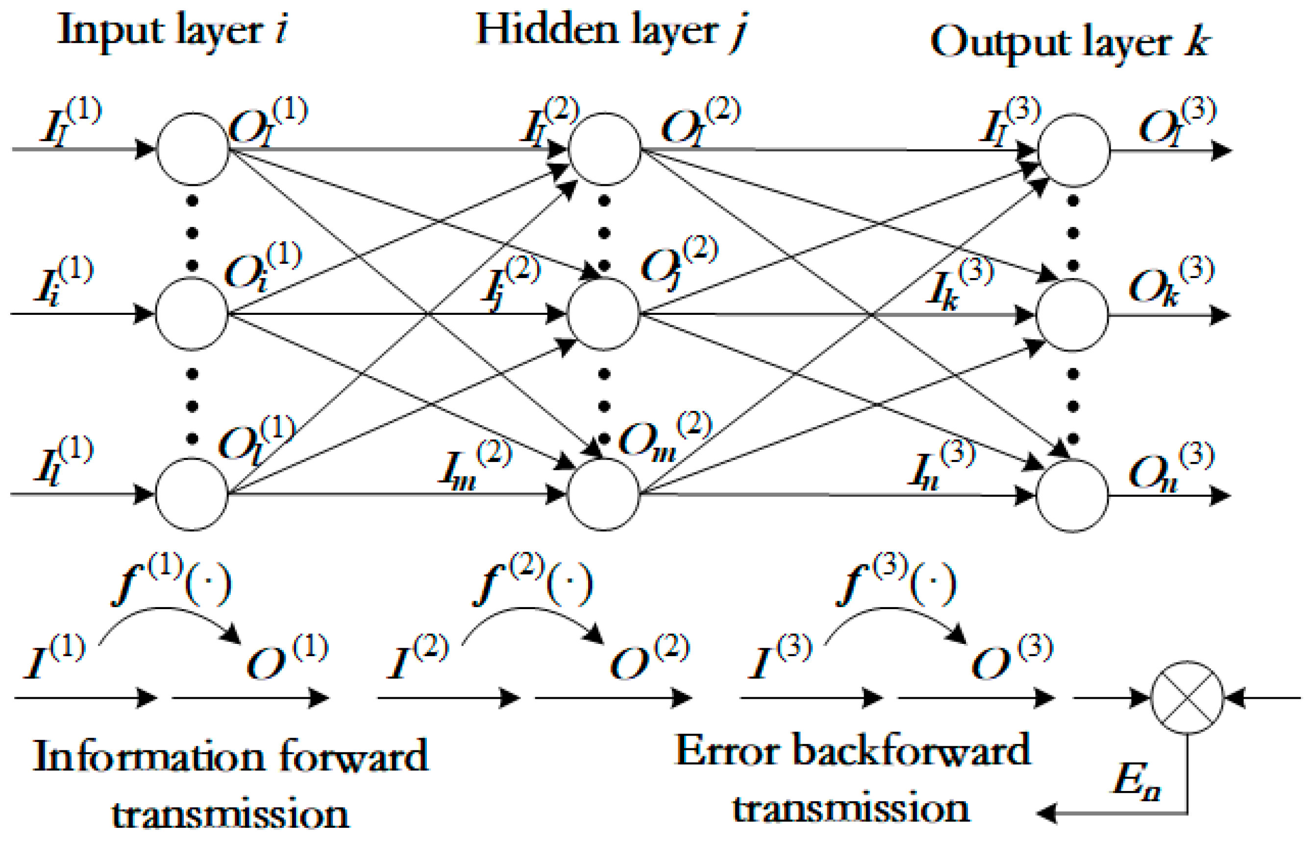
BPNN represents a prevalent algorithm for the training of feedforward neural networks [36]. The methodology employed is initiated by the calculation of the error in the output layer. This is followed by the recursive propagation of this error in a backward direction through the network, with the objective of estimating errors in the preceding layers. The backward propagation is conducted layer-wise until all layer errors have been calculated. Subsequently, the network is trained using gradient descent optimization to minimize the loss function, iteratively adjusting the weights based on these error gradients. It is evident that the widespread use of BPNNs in engineering applications is largely due to their computational efficiency. The typical structural configuration of a BPNN comprises an input layer, one or more hidden layers, and an output layer, as shown in Figure 1.

As illustrated in Figure 1, I denotes the input of the neuron, whilst O denotes the output of the neuron. The excitation functions of the input layer, hidden layer and output layer are represented by f⁽¹⁾(·), f⁽²⁾(·) and f⁽³⁾(·), respectively, where the superscripts (1), (2) and (3) indicate the number of layers in each case.

For P training samples, the input–output relationship of the p-th sample (p = 1, 2, …, P) follows the mathematical representation in

Table 1. Input and output layers.

Input layer	Input	$I_{ip}^{(1)} i=1,2,\cdots l,$	(17)
	Output	$O_{ip}^{(1)}=I_{ip}^{(1)}.$	(18)
Hidden layer	Input	$I_{jp}^{(2)}={\displaystyle \sum _{i=1}^l\left({\omega }_{ji}{O}_{ip}^{(1)}-{\theta }_j\right)},$	(19)
	Output	$O_{jp}^{(2)}=f^{(2)}\left(I_{jp}^{(2)}\right), j=1,2,\cdots ,m.$	(20)
Output layer	Input	$I_{kp}^{(3)}={\displaystyle \sum _{j=1}^m\left({\omega }_{kj}{O}_{jp}^{(2)}-{\theta }_k\right)},$	(21)
	Output	$O_{kp}^{(3)}=f^{(3)}\left(I_{kp}^{(3)}\right), k=1,2,\cdots ,n.$	(22)

where ω_ji is defined as the connection weight from the i-th neuron in the input layer to the j-th neuron in the hidden layer, ω_kj denotes the connection weight from the j-th neuron in the hidden layer to the k-th neuron in the output layer. θ_j is the threshold of the second-layer neurons, and θ_k is the threshold of the third-layer neurons.

.

The BPNN algorithm employs the steepest descent method in nonlinear programming and modifies each weight and threshold of network neurons in the direction of the negative gradient of the error function [37]. As shown in Equation (23), the error function E_n is defined as the sum of the squares of the differences between the expected output and the actual output of the network.

$$E_n(t)={\displaystyle \frac{1}{2P}}{\displaystyle \sum _{p=1}^P{\displaystyle \sum _{k=1}^n{\left(O_{dk}-O_{kp}^{(3)}\right)}^2}},$$

(23)

where O_dk is the expected value of each node in the output layer, k = 1, 2, …, n.

2.3. Research Route

The proposed POD-BPNN methodology integrates the dimensionality reduction capabilities of POD with the predictive capabilities of BPNN to enhance system response prediction efficiency. The workflow comprises the following sequential steps:

Design Space Construction: Firstly, the input and output parameters of the engineering problem are defined. Then, input parameter sampling is achieved, and batch simulation is carried out to generate the training datasets.

Dimensionality Reduction: Based on the training datasets generated, a snapshot matrix is obtained. Then, SVD is applied to the snapshot matrix to extract the dominant basis vectors that capture the primary modes of the high-dimensional system. The optimal coefficients for the basis vectors are determined via least squares optimization, yielding a reduced-order output dataset. This dataset, combined with the original inputs, forms the training dataset for the surrogate model.

Surrogate Model Training: A BPNN surrogate model is trained using the constructed dataset, and its accuracy is validated to ensure compliance with predefined performance criteria.

System Reconstruction and Prediction: The final prediction phase combines the BPNN output with the retained basis modes through a linear reconstruction process, enabling the recovery of high-dimensional system states and rapid response prediction. The systematic workflow of the POD-BPNN methodology is schematically outlined as shown in Figure 2.

3. Structural Physical Field Reconstruction of the Test Section

3.1. Problem Description

3.1.1. Object Description

The test section constitutes the core component of the wind tunnel system, designed to host aerodynamic models and simulate the surrounding flow environment to quantify the effects of gas flow on the tested configuration [38]. Its structural framework employs a truss wall panel design, characterized by cross-sectional dimensions that incorporate a base, a portal frame, a wall panel assembly, a top door, and the side doors, as illustrated in Figure 3.

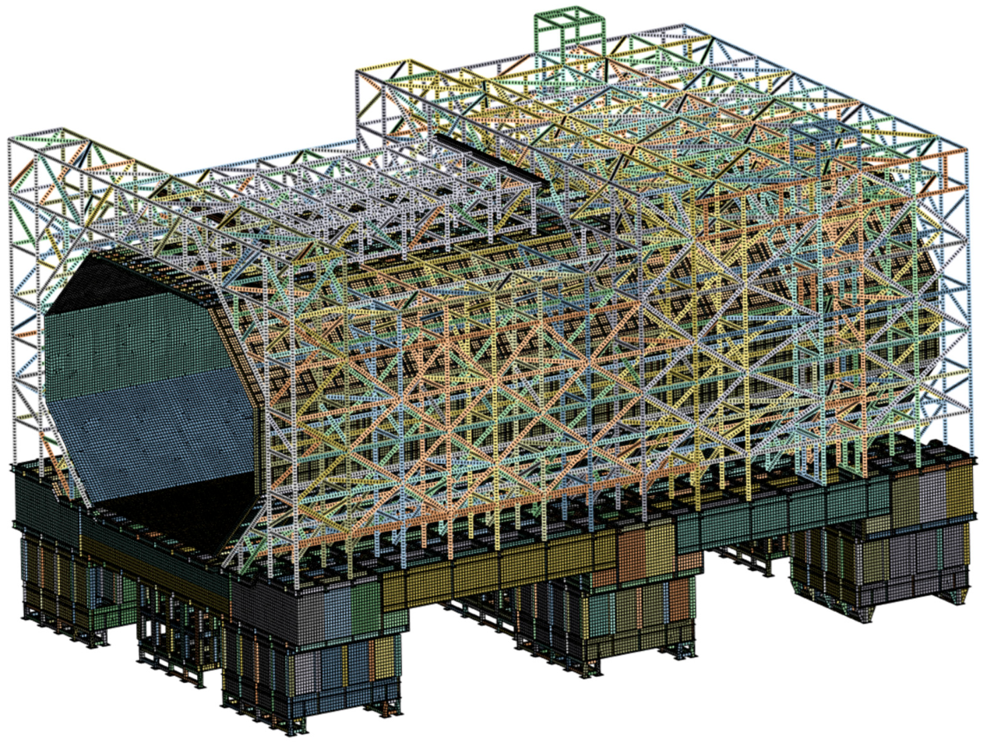
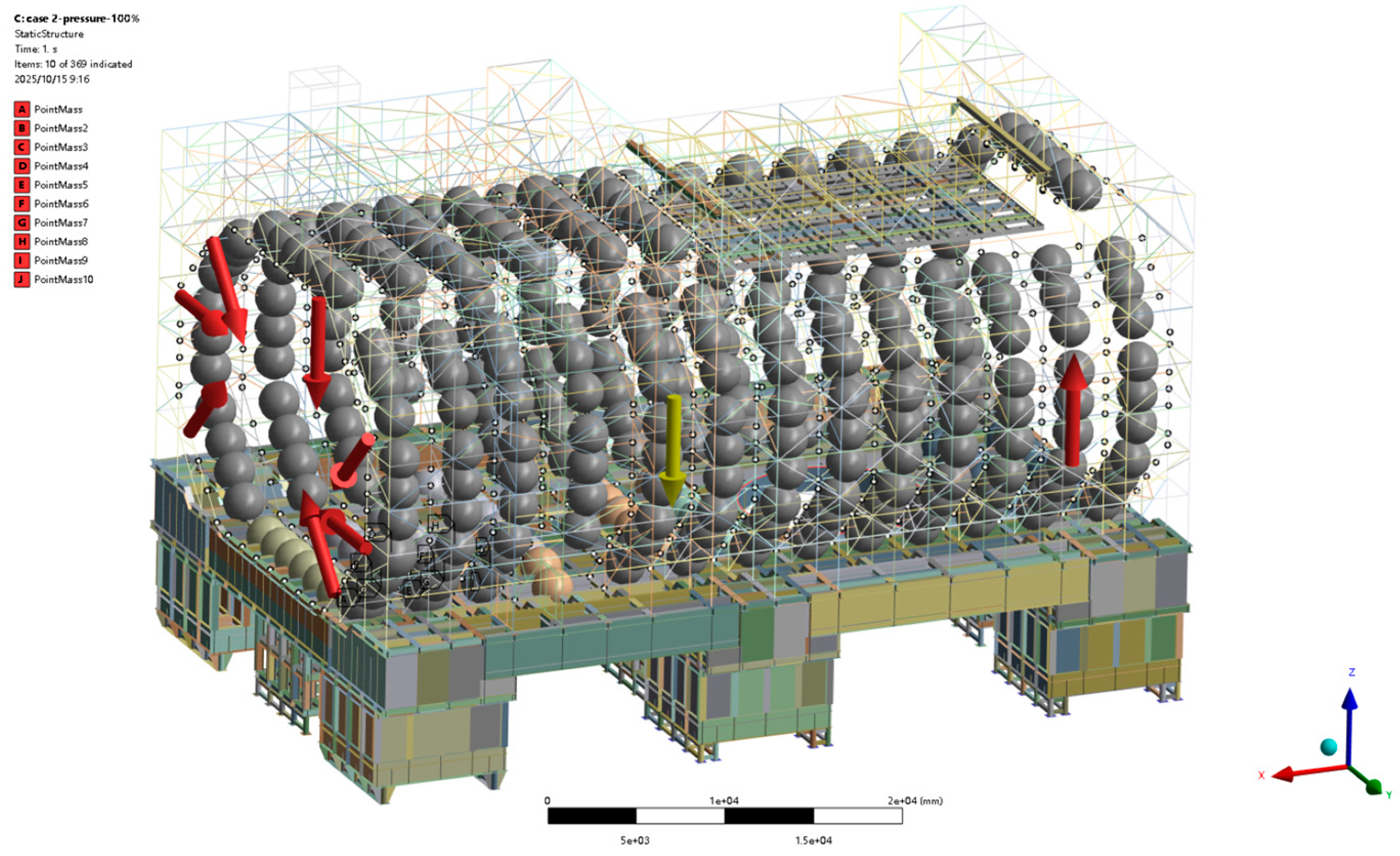
The operational parameters of the wind tunnel primarily depend on the wind speed of the test section, as it typically functions under atmospheric pressure. During operation, the test section must withstand its self-weight and aerodynamic loads induced by airflow. To evaluate its structural performance, FE analysis was conducted to derive stress and displacement responses of the structure. The FE mesh model and associated loading conditions are depicted in Figure 4 and Figure 5. The primary structural components are fabricated from Q355 steel, with material properties specified as shown in

Table 2. Material properties of the test section.

Name	Density	Young’s Modulus	Poisson’s Ratio	Yield Strength	Tension Strength
Parameter value	7850 kg/m3	210 GPa	0.3	355 MPa	470 MPa

. All computations and simulations in this study were performed on an Intel Xeon Gold 6233W platform with 128 GB RAM and NVIDIA Quadro RTX 8000 GPU.

3.1.2. Grid Independence Analysis

Grid independence verification was conducted for the base, the gate frame, and the top door to ensure computational reliability. Three-dimensional FE meshes with varying element sizes were tested for each component, and results were validated using stress distributions and element counts.

(1)

Base grid independence verification

Meshes with element sizes of 150 mm, 100 mm, and 50 mm were analyzed.

Table 3. Grid division and calculation results of the base.

Grid Element Size/mm	Number of Nodes	Number of Elements	Stress/MPa	Stress Growth Rate/%
150	765,085	789,654	27.91	--
100	1,363,016	1,380,220	29.34	5.12
50	5,374,816	5,409,800	30.05	2.42

lists the grid division and calculation results of the base, with the stress distribution as shown in Figure 6. It can be seen from Table 3 and Figure 6 that reducing the element size from 150 mm to 100 mm increases the peak stress by about 5%, while further reduction to 50 mm yields only a 2% change in peak stress. To balance computational efficiency and accuracy, a 50 mm base mesh size was selected, yielding approximately 5.4 million elements.

(2)

Portal frame grid independence verification

Meshes with element sizes of 300 mm, 200 mm, and 100 mm were tested.

Table 4. Grid division and calculation results of the portal frame.

Grid Element Size/mm	Number of Nodes	Number of Elements	Stress/MPa	Stress Growth Rate/%
300	62,874	32,389	27.35	--
200	93,361	47,675	27.35	0
100	184,068	92,986	27.35	0

tabulates the grid division and calculation results of the portal frame, with the stress distribution as shown in Figure 7. It can be seen from Table 4 and Figure 7 that there is no significant change in peak stress when reducing the element size from 300 mm to 200 mm. Thus, the coarser 300 mm mesh size was retained for computational efficiency, resulting in approximately 32,000 elements.

(3)

Top door grid independence verification

Meshes with element sizes of 70 mm, 50 mm, and 30 mm were evaluated.

Table 5. Grid division and calculation results of the top door.

Grid Element Size/mm	Number of Nodes	Number of Elements	Stress/MPa	Stress Growth Rate/%
70	110,253	101,582	77.43	-
50	179,763	168,630	77.80	0.47
30	477,599	458,783	77.94	0.17

enumerates the grid division and calculation results of the top door. It can be seen from Table 5 that when the element size is 50 mm or less, stress increments are less than 0.5%. Therefore, a 50 mm mesh size was chosen to optimize precision and computational resources, resulting in approximately 170,000 elements.

Based on the grid independence verification results, optimized mesh sizes were determined as follows: 50 mm for the base structure, 300 mm for the portal frame, and 50 mm for the top door assembly. The resultant stress distribution contours of the test section under operational loads are presented in Figure 8.

3.1.3. Problem Description for Physical Field Reconstruction

The inverse problem establishes wind velocity distribution within the test section as input parameters while considering resultant stress fields and structural deformations as output responses. The governing mathematical formulation is described by Equations (24)–(26):

$$\mathit{x}=\mathit{v},$$

(24)

$$\mathit{Y}=\left(s,\mathsf{\sigma }\right),$$

(25)

$$\mathit{x}\stackrel{f}{\to }\mathit{Y}.$$

(26)

Through POD-BPNN implementation, Equation (26) undergoes dimensionality reduction to Equation (27).

$$\mathit{x}\stackrel{f}{\to }\mathsf{\alpha }\stackrel{\mathit{S}\approx \stackrel{⌢}{\mathsf{\Phi }}\mathsf{\alpha }}{\to }\mathit{Y}.$$

(27)

This reformulation enables the surrogate model to map physical field parameters to their lower-dimensional orthogonal subspace coefficients, effectively decoupling high-fidelity simulations from optimization processes.

3.2. Snapshot Matrix Construction Methodology

The experimental configuration employed a wind tunnel design-point wind speed of 80 m/s. Ten representative operating conditions were systematically generated through uniform sampling across the operational envelope, forming the complete training dataset as detailed in

Table 6. Design of test section operating conditions.

Operating Conditions	Case 1	Case 2	Case 3	Case 4	Case 5	Case 6	Case 7	Case 8	Case 9	Case 10
Wind speed/m·s−1	16	32	48	64	80	96	112	128	144	160
x/kN	22.5	90.0	202.5	360.0	562.5	810.0	1102.5	1440.0	1822.5	2250.0
y/kN	3.4	13.6	30.6	54.4	85.0	122.4	166.6	217.6	275.4	340.0
z/kN	6.8	27.2	61.2	108.8	170.0	244.8	333.2	435.2	550.8	680.0

Here, x, y, and z denote the aerodynamic load vectors acting on the upper/lower wall panels, left/right wall panels, and vertically diagonal wall panels, respectively. Multi-operational condition simulations are conducted based on predefined working scenarios. Displacement and stress response values at each nodal point are recorded across all conditions, and these data are compiled into the snapshot matrix S.

. Following standard machine learning protocols, cases 3 and 7 were designated as validation benchmarks, with the remaining eight cases comprising the training subset for model development.

3.3. Data Dimensionality Reduction

SVD was applied to the snapshot matrix S using Equation (9), yielding the eigenvalues and associated energy contributions for each mode of the high-dimensional system as shown in

Table 7. Energy contribution ratios corresponding to different orders.

Order r	1	2	3	4	5	6	7	8	9	10
Eigenvalues λ	1,566,246.0	4342.5	523.2	216.4	105.4	22.1	8.8	1.6	0.3	0.2
Cumulative energy proportion I(r)/%	95.85	96.72	97.98	98.56	98.99	99.52	99.98	100.00	100.00	100.00

. Analysis of Table 7 reveals that a modal truncation order (r = 7) achieves a cumulative energy proportion of 99.98%, indicating that seven modes are enough to capture nearly all system features while fulfilling the criterion that the truncated subspace retains energy comparable to the full-order model [39]. Thus, retaining the first seven modes enables projection of the full-order system onto a reduced-order subspace. The first seven POD basis vectors are denoted as $\stackrel{⌢}{\mathsf{\Phi }}$ = {ϕ₁, ϕ₂, ϕ₃, ϕ₄, ϕ₅, ϕ₆, ϕ₇}. Using the approximations defined by Equations (19) and (20), the coefficients corresponding to each basis vector were determined via the least squares method. By combining these seven POD modes with the coefficient matrix α, the original stress/displacement field matrix was reconstructed by recalculating operating conditions at ten sampling points.

3.4. Surrogate Model Training

(1)

Neural network architecture

A BPNN model was trained to predict the stress and deformation fields of the test section. Multiple architectural configurations and hyperparameters were systematically explored to achieve high-precision results. Architectural variations included the number of hidden layers and activation functions, while hyperparameters such as batch size and learning rate were tuned.

The batch size and learning rate are evaluated using mean relative error (MRE) and root mean square error (RMSE) [40], defined in Equations (28) and (29).

$$\mathrm{MRE}={\displaystyle \frac{1}{n}}{\displaystyle \sum }_{i=1}^n\left(\left|{\displaystyle \frac{x_i-{\widehat{x}}_i}{x_i}}\right|\times 100\%\right)$$

(28)

$$\mathrm{RMSE}=\sqrt{{\displaystyle \frac{1}{n}}{\displaystyle \sum }_{i=1}^n{(x_i-{\widehat{x}}_i)}^2}$$

(29)

where n denotes the sample size, x_i represents the true value of the i-th samples, while ${\widehat{x}}_i$ is the corresponding predicted value.

Table 8. The computational accuracy under different batch sizes and learning rates.

Batch Sizes	Learning Rate η	MRE/%	RMSE/%
32	0.001	0.56	0.021
32	0.0001	0.18	0.018
64	0.001	0.11	0.016
64	0.0001	0.28	0.028

summarizes the accuracy of reduced-order models trained with varying batch sizes and learning rates. Results reveal a positive correlation between batch size and both MRE and RMSE. When the batch size reaches 64, model accuracy surpasses 99.9%. However, smaller learning rates η lead to reduced accuracy due to overfitting [41]. Consequently, optimal training parameters were selected as batch size = 64 and learning rate η = 0.001, balancing predictive performance and generalization.

Table 9. Percentage error for different layers.

Framework	Two Layers	Three Layers	Four Layers
Stress peak percentage error/%	0.81	1.22	1.65
Deformation valley peak percentage error/%	2.59	2.67	2.74

summarizes the influence of network layer count on the prediction accuracy of BPNN models. Results indicate that exceeding two layers increases the risk of overfitting, leading to higher prediction errors.

Common activation functions for neural network surrogate models include sigmoid, tanh, and ReLU, whose formulations are defined in Equations (30)–(32) [42,43].

Table 10. Percentage error for different activation functions.

Activation Function	Sigmoid (x)	Tanh (x)	ReLU (x)
Stress peak percentage error/%	2.22	3.16	2.22
Deformation valley peak percentage error/%	0.96	4.24	2.23

presents the impact of these functions on surrogate model accuracy. It can be seen that neural networks employing the sigmoid function achieve higher accuracy than those using alternative activation functions.

$$\mathrm{sigmoid}(x)={\displaystyle \frac{1}{1+exp(-x)}},$$

(30)

$$\tan \mathrm{h}(x)={\displaystyle \frac{1-exp(-2x)}{1+exp(-2x)}},$$

(31)

$$\mathrm{ReLU}(x)=max(x,0).$$

(32)

(2)

Loss function

The SmoothL1Loss function (abbreviated as LL [44]) constitutes a hybrid of L1Loss and L2Loss. It addresses the non-smoothness and convergence challenges of L1Loss during later training stages while mitigating L2Loss’s susceptibility to gradient explosion and outlier sensitivity. Specifically, the LL function maintains bounded gradients for small prediction errors and reduces sensitivity to large errors, thereby enhancing overall stability. Its mathematical formulation is provided in Equation (33).

$$\mathrm{LL}={\displaystyle \frac{1}{n}}{\displaystyle {\sum }_{i=1}^n\left\{\begin{array}{ll}0.5{\left(y_i-{\widehat{y}}_i\right)}^2,& \mathrm{if}\left|y_i-{\widehat{y}}_i\right|<1\\ \left|y_i-{\widehat{y}}_i\right|-0.5,& \begin{array}{cc}\mathrm{otherwise}& \end{array}\end{array}\right.}.$$

(33)

where y_i is the actual value of the i-th sample, and ${\widehat{y}}_i$ is its predicted counterpart.

Based on the analysis of neural network parameters and architectures, a BPNN model with the following configuration was selected (

Table 11. BPNN hyperparameters.

Hidden Layer Number	Neuro Number		Learning Rate	Epoch	Batch Size	Activation Function	Loss Function	Optimizer
2	24	48	0.01	1000	64	Sigmoid	L1	AdamW

): batch size 64, learning rate 0.01, two hidden layers, Sigmoid activation function, and SmoothL1Loss. The initial weight coefficient is set to 1, and the upper limit for the number of iterations is set to 10,000. Figure 9 depicts the neural network architecture. Accordingly, the trained surrogate model successfully reconstructed the displacement and stress fields of the wind tunnel test section structure, as shown in Figure 10.

Table 12. Comparison of calculation times for POD-BPNN and FE simulations.

Type	Number of Model Grids	Calculation Time/s
FE simulations	852,112	960
POD-BPNN	852,112	0.31

presents the comparison of calculation times for POD-BPNN and FE simulations. As shown in Table 12, the POD-BPNN model achieves a computational speed improvement of three orders of magnitude over FE simulations for physical field reconstruction. This significantly accelerates predictions of structural performance in wind tunnel test sections and meets the real-time requirements for structural condition monitoring systems.

4. Results and Discussion

4.1. Model Validation

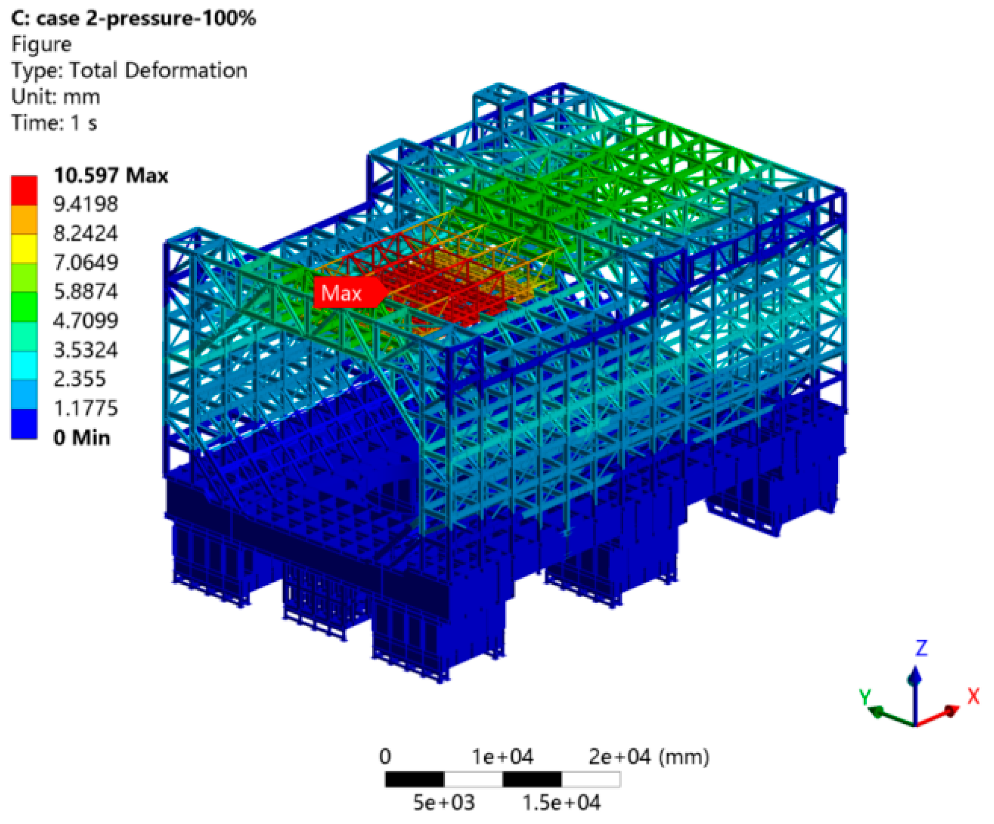
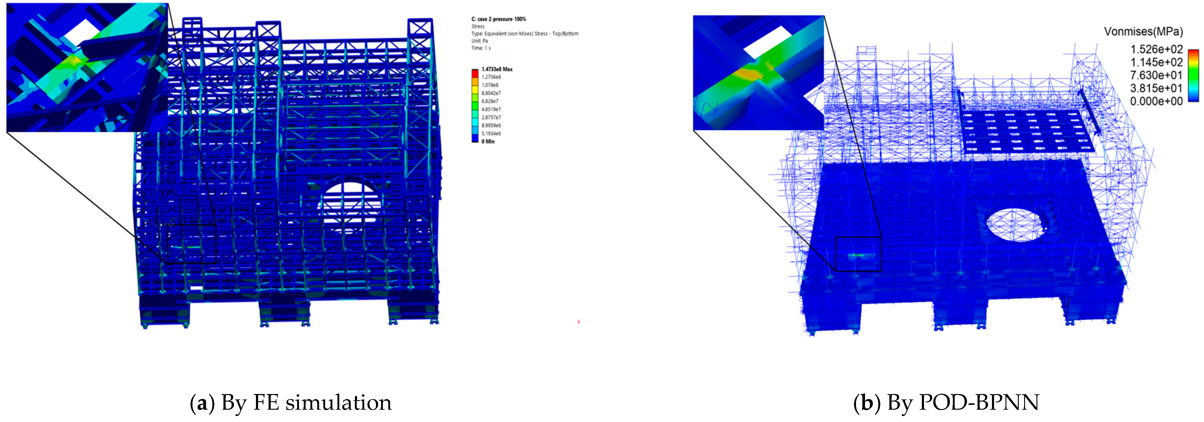
To evaluate the accuracy of the established POD-BPNN model, case 7 from the validation dataset (in Table 6) was selected for testing. According to the prevailing pressure vessel design codes, structural deformation and stress amplitude are the most common indicators for evaluating the operational safety performance of equipment design. A comparison of the amplitude results with the average values of adjacent regions provides an effective means to assess the predictive capability of the model. Figure 11 compares the deformation field of the test section by FE simulation and POD-BPNN reconstruction, while Figure 12 presents the corresponding stress field comparison.

It can be seen from Figure 11 that both methods exhibit consistent deformation distributions, with localized high deformations in the top gate region. The FE simulation predicts a maximum deformation of 10.59 mm, whereas the POD-BPNN model yields 10.92 mm, resulting in a relative error of 3.05%. A comparative domain analysis focused on 4368 nodes near the maximum deformation point revealed an average deformation of 9.03 mm (by FE) and 9.22 mm (by POD-BPNN), with a relative error of 2.06%.

It can be seen from Figure 12 that the FE simulation and POD-BPNN model predict maximum stresses of 147.33 MPa and 152.6 MPa, respectively, yielding a relative error of 3.58%. A domain analysis of 1921 nodes near the maximum stress point showed average stresses of 66.5 MPa (by FE) and 69.7 MPa (by POD-BPNN), with a relative error of 4.74%.

Validation results confirm that the proposed POD-BPNN model achieves prediction accuracies exceeding 95% for the structural deformation and stress predictions in the test section, thereby fulfilling the precision requirements for wind-tunnel-structure condition monitoring.

In modern wind tunnel facility design and construction, intelligent health management systems based on multidimensional sensor-based monitoring have become essential technical components for ensuring safe operational performance [3]. During the commissioning phase, the dynamic similarity between reduced-order models (ROMs) constructed from simulation data and actual physical systems is enhanced through a coupling correction framework that integrates sparse sensor data acquired from the health monitoring system. This data-model synergistic analysis approach enables the integration of measured operational data as input parameters into the deployed hybrid reduced-order framework, thereby achieving quasi-real-time, system-wide condition monitoring and fault prediction capabilities for complex wind tunnel installations.

As evidenced by the validation results, the prediction accuracy for structural deflection parameters (both amplitude and regional averages) consistently surpasses that of stress predictions. Finite element analysis contour plots reveal that deflection fields exhibit spatially extensive variations with distinct gradient characteristics between pronounced deformation regions and adjacent areas. In contrast, the von Mises stress fields demonstrate relatively uniform distribution patterns with smaller numerical disparities between different zones. This inherent disparity results in lower modal participation ratios for stress predictions compared to deflection predictions when identical truncation orders are applied during system reduction processes, consequently limiting their predictive fidelity.

The present study highlights the limitations of employing uniform truncation criteria when constructing reduced-order models for different response variables within the same physical system. Future research should prioritize developing modal truncation strategies tailored to specific output quantities, such as displacements and stresses, to optimize the trade-off between prediction accuracy and computational efficiency. This aspect remains an underexplored area offering significant potential for improvement.

4.2. Generalization Performance Analysis

The surrogate model was trained using a dataset encompassing wind speeds from 16 m/s to 160 m/s (in Table 6). Within this training range, the POD-BPNN model demonstrated high accuracy in approximating the original FE model. To evaluate its extrapolation capability, three out-of-distribution operating conditions (176 m/s, 192 m/s, and 208 m/s) were tested via uniform sampling. The relative errors for maximum stress and deformation predictions for these extrapolated cases are summarized as shown in

Table 13. Prediction results of operating conditions outside the training range.

Operating conditions/m·s−1	48	112	176	192	208
Maximum deformation relative error/%	2.73	2.98	8.54	13.56	17.65
Maximum stress relative error/%	2.88	3.41	9.63	15.32	18.28

.

It can be seen from Table 13 that the reduced-order model maintains relative errors below 4% for design conditions within the training range. However, prediction accuracy progressively declines as operating conditions deviate further from the original design space, with errors increasing for extrapolated cases.

The performance degradation exhibited by the POD-BPNN hybrid framework under extrapolative operating conditions can be attributed to two primary factors: first, the information loss inherent to the POD-based reduced-order modeling process due to truncation effects; second, the generalization limitations imposed by the black-box nature of the BPNN surrogate model. It is well-recognized that data-driven surrogate models inherently possess black-box characteristics, with their predictive mechanisms and operational processes remaining poorly understood. These models consistently demonstrate suboptimal generalization capabilities when applied beyond their training domains. Consequently, establishing methodologies to precisely identify the origin of generalization errors and quantify their impact on prediction outcomes represents a critical research direction to enhance the framework’s predictive robustness. This constitutes a promising avenue for advancing the applicability of hybrid reduced-order modeling approaches.

4.3. Model Extension Performance Verification

The proposed POD-BPNN framework was extended to reconstruct the pressure distribution across the wind tunnel fan section’s flow field. The model was trained using 42 datasets generated by varying fan rotational speed and flow quantity (as input parameters) and mapping to corresponding pressure distributions (as output parameters).

CFD simulations were performed under the ideal gas assumption, with the moving and stationary blades modeled as single-channel flows. Rotational periodicity was applied to the moving blades, while mixed plane methods were implemented at three critical interfaces: between the moving blades and the forward transition section, between the moving and stationary blades, and between the stationary blades and the aft transition section. Open pressure inlet and mass flow outlet boundary conditions were prescribed, and steady-state flow field analyses were conducted using the k-ω turbulence model. After verifying mesh independence through convergence studies, the computational mesh configuration comprised approximately 14 million elements to ensure solution accuracy while maintaining numerical efficiency.

Under the operating condition of 140 rpm fan speed and 6700 kg/s flow quantity, the POD-BPNN model computed the pressure distribution in 1.14 s, compared to 7200 s required for a single CFD simulation run. Figure 13 compares the pressure cloud images from both models. The maximum pressure predictions were 122.83 kPa (by POD-BPNN) versus 122.50 kPa (by CFD), yielding a relative error of 0.26%; minimum pressure values showed 88.76 kPa (by POD-BPNN) versus 89.16 kPa (by CFD), with a relative error of 0.45%. These results confirm that the proposed model satisfactorily fulfills both precision and real-time operational requirements for wind tunnel flow field monitoring.

5. Conclusions

To address the holistic and real-time demands of wind tunnel condition monitoring, this study proposes a POD-BPNN method for wind tunnel physical field reconstruction. This approach combines POD and BPNN. By transforming high-dimensional systems into low-dimensional ones through POD, the computational cost of training a neural network surrogate model could be significantly reduced while maintaining accuracy.

Using the reconstruction of stress and displacement fields in a wind tunnel test section as a case study, this research evaluates learning rates and batch sizes via MRE and RMSE. Additionally, it examines the effects of varying neural network architectures and activation functions on the model’s precision. Results demonstrate that the POD-BPNN achieves reconstruction accuracies exceeding 95% for both stress and displacement fields in the test section, with prediction times reduced by three orders of magnitude compared to FE analysis. This confirms its ability to meet the dual requirements of precision and real-time performance for wind tunnel structural condition monitoring.

The proposed POD-BPNN model was applied to reconstruct the flow field of a wind tunnel fan section, achieving a pressure distribution prediction error of less than 1% compared to CFD simulations. Additionally, the model completed predictions in under 1.5 s per instance, fulfilling both accuracy and real-time requirements for wind tunnel condition monitoring.

Through generalization performance validation, the current study identified that the model demonstrates a significant decline in prediction accuracy under test conditions beyond the training scope. Future research should prioritize exploring physics-informed approaches integrating physical constraint conditions (e.g., governing equations) into deep learning frameworks to enhance the model’s generalization capacity across complex operational scenarios. Notably, while this study has achieved preliminary quasi-real-time monitoring of flow field distribution and structural state parameters, a comprehensive fault diagnosis system remains underdeveloped. Subsequent research could integrate typical fault characteristic databases from wind tunnel assemblies with expert knowledge to construct a physics-constrained intelligent diagnostic model (Physical Constraint-based Intelligent Diagnostic Model), thereby enabling a paradigm shift from data monitoring to predictive fault identification. It is evident that, despite the research achieving rapid reconstruction of physical fields through systematic dimensionality reduction and surrogate modeling, a discrepancy remains in terms of response speed in comparison to the real-time synchronization, which is necessary for the construction of equipment digital twins. The main structures of the wind tunnels studied all belong to symmetrical structures. When the load is evenly distributed, the symmetry of the structure can be utilized to significantly shorten the time for cloud image reconstruction and further enhance the response speed.

Furthermore, the proposed method has achieved breakthroughs in real-time performance and data integrity, providing robust support for digital space simulation in equipment digital twins. However, it should be emphasized that the full realization of an equipment digital twin system necessitates breakthroughs in the following dimensions: (1) multi-timescale coupling between operational control logic models and physical space models; (2) bidirectional driving and real-time interaction technologies for virtual–physical data; and (3) collaborative optimization of multimodal data fusion and intelligent decision-making systems. Consequently, future research should concentrate on multidimensional synergetic innovation in digital twin systems, leveraging interdisciplinary methodologies to achieve deep integration and intelligent evolution between virtual and physical spaces.

References

1. Lai, H.; Zhu, C.J.; Chen, W.H.; Liao, D.; Sun, D. Key technology for mechanical design in large-scale cryogenic wind tunnel. J. Exp. Fluid Mech. 2022, 36, 19–26. (In Chinese) [Google Scholar]
2. Yang, X.S.; Guo, S.C.; Du, L.Q.; Gai, W.; Chen, J. Control System for Certain Type Aero-acoustic Wind Tunnel. Ordnance Ind. Autom. 2020, 39, 54–59. (In Chinese) [Google Scholar]
3. Wang, Q.; Li, Z.S.; Li, S.C.; Du, L. Structural health monitoring system for large low speed wind tunnel. Ordnance Ind. Autom. 2024, 43, 18–22+41. (In Chinese) [Google Scholar]
4. Yang, X.S.; Liu, Z.Z.; Guo, S.C. Simulation and test of torsional vibration of compressor for a continuous transonic wind tunnel. Comput. Meas. Control 2024, 32, 28–34. [Google Scholar]
5. Yang, Y.; Yang, Z.; Yan, X.; Yan, S.; Liu, B.; Ding, H. Multi-fidelity Surrogate Model Based Wind Tunnel Structure Design Optimization. In Proceedings of the 16th International Conference on Advanced Computational Intelligence, ICACI 2024, Zhangjiajie, China, 16–19 May 2024; Institute of Electrical and Electronics Engineers Inc.: New York, NY, USA, 2024; pp. 72–78. [Google Scholar]
6. Yang, W.G.; Wang, R.; Yin, Y.T.; Chen, W. Structure design and research of 5.5 m × 4 m aeroacoustics wind tunnel. Acta Aeronaut. Astronaut. Sin. 2023, 44, 127711. (In Chinese) [Google Scholar]
7. Wei, Y.; Zhou, H.; Zhang, T.; Wang, S. Inverse identification of multiple temporal sources releasing the same tracer gaseous pollutant. Build. Environ. 2017, 118, 184–195. [Google Scholar] [CrossRef]
8. Lumley, J.L. The Structure of inhomogeneous turbulent flows. In Atmospheric Turbulence and Radio Wave Propagation; Yaglom, A.M., Tartarsky, V.I., Eds.; Defense Technical Information Center: Fort Belvoir, VA, USA, 1967; pp. 166–177. [Google Scholar]
9. Wei, Y. A POD-Based Inverse Method to Promptly Design the Enclosed Environment; Dalian University of Technology: Dalian, China, 2019. (In Chinese) [Google Scholar]
10. Sirovich, L. Turbulence and the dynamics of coherent structures. I—Coherent structures. II—Symmetries and transformations. III—Dynamics and scaling. Q. Appl. Math. 1987, 45, 573–582. [Google Scholar] [CrossRef]
11. Cazemier, W.; Verstappen, R.W.C.P.; Veldman, A.E.P. Proper orthogonal decomposition and low-dimensional models for driven cavity flows. Phys. Fluids 1998, 10, 1685–1699. [Google Scholar] [CrossRef]
12. Ravindran, S.S. Reduced-order adaptive controllers for fluid flows using POD. J. Sci. Comput. 2000, 15, 457–478. [Google Scholar] [CrossRef]
13. Graham, W.R.; Peraire, J.; Tang, K.Y. Optimal control of vortex shedding using low-order models. Part I—Open-loop model development. Int. J. Numer. Methods Eng. 1999, 44, 945–972. [Google Scholar] [CrossRef]
14. Feng, X.Y.; Bai, F.; Ding, H.; Tao, W. An improved POD-Galerkin method for rapid prediction of three-dimensional temperature field for an IGBT module. Int. Commun. Heat Mass Transf. 2024, 152, 107241. [Google Scholar] [CrossRef]
15. Lu, S.Q.; Papadakis, G. Flow reconstruction around a surface mounted prism from sparse velocity and or sca1ar measurements using a combination of pod and a data driven estimator. Flow Turbul. Combust. 2023, 110, 1059–1090. [Google Scholar] [CrossRef]
16. Nkemnole, E.B.; Wulu, J.T.; Osubu, I. Application of K-nearest neighbours and long-short-term memory models using hidden markov model to predict inflation rate and transition patterns in nigeria. J. Appl. Sci. Environ. Manag. 2024, 28, 1913–1925. [Google Scholar] [CrossRef]
17. He, H.T.; Liu, Y.B. Full system model of flywheel rotor based on BP neural network. J. North China Electr. Power Univ. 2025, 52, 99–106. [Google Scholar]
18. Ma, F.; Zhang, Q.; Lai, P.J.; Yue, Y. BP neural network-based quantitative classification model for safety in experimental flight training. Acta Aeronaut. Astronaut. Sin. 2024, 45, 529957. (In Chinese) [Google Scholar]
19. Liu, Q.; Liu, B.; Pan, Y.C.; Zhao, Y.; Wang, K.; Deng, H.; Gong, X. Mechanical properties of magnetorheological shear thickening fluid and its application in dampers. Smart Mater. Devices 2025, 1, 202405. [Google Scholar] [CrossRef]
20. Yun, G.L.; Hu, Z.W. Triaxial tactile sensing for next-gen robotics and wearable devices. Smart Mater. Devices 2025, 1, 202518. [Google Scholar] [CrossRef]
21. Mohan, A.T.; Gaitonde, D.V. A deep learning based approach to reduced order modeling for turbulent flow control using LSTM neural networks. arXiv 2018, arXiv:1804.09269. [Google Scholar] [CrossRef]
22. Zhang, W.M.; Feng, D.D.; Ge, Y.J. Nonlinear aerodynamic force model of bridge based on deep learning. Bridge Constr. 2023, 53, 16–24. (In Chinese) [Google Scholar]
23. Hao, Y.Q.; Zhao, D.Z.; Li, W.B.; Kong, M.; Liu, S. POD-BPNN prediction model and uncertainty quantification of aircraft icing conditions. J. Nanjing Univ. Aeronaut. Astronaut. 2023, 55, 302–310. (In Chinese) [Google Scholar]
24. Jia, X.Y.; Gong, C.L.; Li, C.N. Fast flow simulation method based on POD and BPNN. J. Northwest. Polytech. Univ. 2021, 39, 1212–1221. (In Chinese) [Google Scholar] [CrossRef]
25. Du, X.Q.; Shen, X.Y.; Dong, H.T.; Chen, T. A wind-pressure reconstruction method of POD-BPNN using measurement-point clustering. J. Civ. Eng. 2024, 57, 11–21. (In Chinese) [Google Scholar]
26. Guan, K.G.; Su, W.Y.; Cui, S.; Zhang, W.; Ma, H. POD-BPNN prediction on the three-dimensional complex flow field of hypersonic waverider forebody/inlet. J. Aerosp. Power 2025, 40, 20220536. (In Chinese) [Google Scholar]
27. Kang, Y.; Tian, G.; Huang, Y.; Qin, S.; Huang, Q.; Yuan, Y.; Zhou, Y. Fast prediction and inverse modeling for parameterized depressurization from a CO2 vessel using POD-BPNN reduced-order method. Prog. Nucl. Energy 2025, 183, 105684. [Google Scholar] [CrossRef]
28. Min, G.Y.; Jiang, N.B. Flow fields prediction for data-driven model of parallel twin cylinders based on POD-RBFNN and POD-BPNN surrogate models. Ann. Nucl. Energy 2024, 199, 110342. [Google Scholar] [CrossRef]
29. Hu, J.X.; Gou, J.J.; Gong, C.L. An enhanced temperature field inversion model by POD-BPNN-GA method for a 3D wing with limited sensors. Int. Commun. Heat Mass Transf. 2025, 164, 108778. [Google Scholar] [CrossRef]
30. Chen, F.; Kang, W.; Shu, Z.; Li, Q.; Li, Y.; Chen, Y.F.; Zhou, K. Predicting roof-surface wind pressure induced by conical vortex using a BP neural network combined with POD. Build. Simul. 2022, 15, 1475–1490. [Google Scholar] [CrossRef]
31. Yan, H.; Wang, Y.; Yan, Y.; Cui, J. Physics-informed neural network for flow prediction based on flow visualization in bridge engineering. Atmosphere 2023, 14, 759. [Google Scholar] [CrossRef]
32. He, X.; Huang, B.; Peng, L.; Chen, J. Studies on submersible short-circuit blowing based on orthogonal experiments, back propagation neural network prediction, and pearson correlation analysis. Appl. Sci. 2024, 14, 10321. [Google Scholar] [CrossRef]
33. Wang, H.; Du, X.X.; Hu, Y.L. Investigation on the reduced-order model for the hydrofoil of the blended-wing-body underwater glider flow control with steady-stream suction and jets based on the POD method. Actuators 2024, 13, 194. [Google Scholar] [CrossRef]
34. Wu, P.; Ji, L.; Yuan, W.; Liu, Z.; Tang, T. A digital twin framework embedded with POD and neural network for flow field monitoring of push-plate kiln. Future Internet 2023, 15, 51. [Google Scholar] [CrossRef]
35. Qin, W.J. Large Eddy Simulation and POD Analysis of in-Cylinder Turbulent Flow and Its Cycle-to-Cycle Variations in IC Engines; Dalian University of Technology: Dalian, China, 2014. (In Chinese) [Google Scholar]
36. Baum, E.B. Generalizing back propagation to computation. In Proceedings of the Neural Networks for Computing, Snowbird, UT, USA, 13–16 April 1986; pp. 47–52. [Google Scholar]
37. Wang, Z.W. Structural Vibration Based on BP Neural Network Algorithm Research on Modal Fuzzy Control; North China University of Science and Technology: Beijing, China, 2020. (In Chinese) [Google Scholar]
38. Zhang, W.G.; Tang, M.; Wu, J.; Peng, X.; Zhang, G. Overview of wind tunnel test research on tiltrotor aircraft. Acta Aeronaut. Astronaut. Sin. 2024, 45, 530114. (In Chinese) [Google Scholar]
39. Qiu, Y.S.; Bai, J.Q.; Hua, J. Flow field estimation method based on proper orthogonal decomposition and surrogate model. Acta Aeronaut. Astronaut. Sin. 2013, 34, 1249–1260. (In Chinese) [Google Scholar]
40. Chen, G.; Li, D.; Zhou, Q.; Da Ronch, A.; Li, Y. Efficient aeroelastic reduced order model with global structural modifications. Aerosp. Sci. Technol. 2018, 76, 1–13. [Google Scholar] [CrossRef]
41. Gunawardana, A.; Shani, G. A survey of accuracy evaluation metrics of recommendation tasks. J. Mach. Learn. Res. 2009, 10, 2935–2962. [Google Scholar]
42. Liu, X.Y.; Di, X.G. TanhExp: A smooth activation function with high convergence speed for lightweight neural networks. IET Res. J. 2021, 15, 136–150. [Google Scholar] [CrossRef]
43. Pratiwi, H.; Windarto, A.P.; Susliansyah, S.; Aria, R.R.; Susilowati, S.; Rahayu, L.K.; Fitriani, Y.; Merdekawati, A.; Rahadjeng, I.R. Sigmoid activation function in selecting the best model of artificial neural networks. J. Phys. Conf. Ser. 2020, 1471, 012010. [Google Scholar] [CrossRef]
44. Mikulic, J.; Prebezac, D. Accounting for dynamics in attribute-importance and for competitor performance to enhance reliability of BPNN-based importance–performance analysis. Expert Syst. Appl. 2012, 39, 5144–5153. [Google Scholar] [CrossRef]
Figure 1. The typical structure of the BPNN.
Symmetry 17 01923 g001
Figure 2. Flowchart of POD-BPNN wind tunnel condition monitoring process.
Symmetry 17 01923 g002
Figure 3. Schematic image of the structural composition of the test section.
Symmetry 17 01923 g003
Figure 4. Grid division image of the test section.
Symmetry 17 01923 g004
Figure 5. Schematic image of aerodynamic load application in the test section.
Symmetry 17 01923 g005
Figure 6. Stress distribution of the base under different element sizes.
Symmetry 17 01923 g006
Figure 7. Stress distribution of the portal frame under different element sizes.
Symmetry 17 01923 g007
Figure 8. Stress distribution of the test section.
Symmetry 17 01923 g008
Figure 9. The neural network architecture.
Symmetry 17 01923 g009
Figure 10. Reconstructed cloud image by POD-BPNN.
Symmetry 17 01923 g010
Figure 11. Displacement cloud image of the test section.
Symmetry 17 01923 g011
Figure 12. Stress cloud image of the test section.
Symmetry 17 01923 g012
Figure 13. Pressure cloud image of the fan section.
Symmetry 17 01923 g013