Short-Term Road Traffic Flow Prediction Based on the KAN-CNN-BiLSTM Model with Spatio-Temporal Feature Integration

Abstract

Short-term traffic flow prediction is a critical component of efficient management in Intelligent Transportation Systems (ITS), providing real-time travel guidance for commuters and supporting informed decision-making by transportation authorities. To address the current challenges of insufficient prediction accuracy and excessive reliance on time-series features, we propose a spatio-temporal feature-integrated short-term traffic flow prediction model named KAN-CNN-BiLSTM. In this model, traffic flow data from the target road segment and its two adjacent segments are jointly fed into the model to fully leverage spatio-temporal features for prediction. Subsequently, a Convolutional Neural Network (CNN) extracts spatial features from the combined traffic flow data. To overcome the limitation of traditional LSTMs, which can only process unidirectional time series, we introduce a bidirectional long short-term memory network (BiLSTM) with symmetric time series extraction capability. This enables simultaneous capture of historical and future traffic flow dependencies. Finally, we replace the conventional fully connected network with a Kolmogorov–Arnold network (KAN) to enhance the representation of complex nonlinear features. Experimental results using traffic flow data from the UK Highways Agency website demonstrate that the KAN-CNN-BiLSTM model outperforms existing mainstream methods, achieving superior prediction accuracy and minimal error. The model’s MAE, RMSE, MAPE, and R² values are 27.4696, 40.3923, 8.65%, and 0.9615, respectively.

1. Introduction

In recent years, with rapid socioeconomic development, the number of private vehicles has continued to increase, placing unprecedented pressure on urban transportation systems. Traffic congestion has become one of the most critical urban transportation challenges worldwide, not only reducing travel efficiency but also severely impacting economic development, environmental quality, and public health [1]. For example, traffic congestion leads to fuel wastage, increased exhaust emissions, and frequent traffic accidents. According to statistics, traffic congestion causes an annual economic loss of approximately USD 120 billion in the U.S. [2]. Meanwhile, studies have also shown that prolonged traffic congestion hinders urban development, weakens agglomeration effects, and reshapes regional economic structures, thereby undermining sustainable economic growth [3]. Against this backdrop, Intelligent Transportation Systems (ITS) have been widely recognized as an effective means of alleviating traffic congestion, and accurate traffic flow prediction serves as a fundamental basis for ITS to achieve efficient management [4].

Traffic flow prediction essentially involves predicting fundamental traffic parameters such as volume, speed, and occupancy rate. Current mainstream research focuses on forecasting road traffic volume [5]. Traffic volume typically refers to the number of vehicles passing through a specific road section or segment within a given time period. Traffic flow prediction can be categorized into long-term, medium-term, and short-term forecasts according to the forecast horizon. Among these, the objective of short-term forecasting is to predict road traffic volume over the next 15 min period based on real-time traffic conditions [6]. Short-term traffic flow prediction not only provides drivers with more timely information on road conditions but also assists traffic managers in flexibly adjusting management strategies. These include optimizing traffic signal timing, implementing tidal lanes, or enforcing time-based speed limits. Such applications can effectively alleviate congestion within a short timeframe and improve traffic flow efficiency. Therefore, conducting high-precision short-term traffic flow prediction research holds practical significance for improving traffic safety and traffic flow efficiency, while also possessing important strategic value for the sustainable development of urban transportation.

At present, most existing studies focus on traffic flow prediction for individual road segments, relying heavily on the characteristics of the segment itself while neglecting the flow correlations with adjacent segments [5]. In reality, road traffic constitutes a real-time, nonlinear, and non-stationary stochastic process, with significant uncertainty inherent in the flow of a single road segment. Due to the pronounced spatial correlation of traffic flow, changes in flow on adjacent segments affected by external events—such as traffic accidents or equipment failures—inevitably propagate to the target segment, thereby impacting prediction outcomes. In the field of traffic flow prediction, models such as BPNN, CNN, GNN, GRU, LSTM are widely adopted and serve as mainstream baseline methods [7]. However, these models have inherent limitations in their architecture and feature extraction capabilities, which constrain further improvements in prediction accuracy. BPNN is prone to local optima and exhibits slow convergence. CNN excels at extracting spatial features and identifying spatial correlations between road segments, but struggles with temporal modeling and capturing long-term dependencies. GNNs effectively model spatial dependencies with good scalability, yet they struggle to capture temporal features and incur high computational costs. GRUs are suitable for modeling short-to-medium-term dependencies but struggle with handling ultra-long-term temporal relationships. LSTMs excel at extracting long-term temporal features and are well-suited for complex traffic flow prediction tasks, but have difficulty capturing spatial correlations among road segments in the traffic network.

To address the issues of insufficient prediction accuracy and excessive reliance on time-series features in current traffic flow forecasting, we employ LSTM as the base model for modeling and predicting short-term traffic flow on road segments. Building upon this foundation, we propose a spatiotemporal feature-integrated short-term traffic flow prediction model named KAN-CNN-BiLSTM. Unlike most current studies that rely primarily on the Transformer to capture dependencies [8], our approach employs a CNN and a BiLSTM to extract both the spatial correlations between adjacent road segments and the bidirectional temporal dependencies. Moreover, this study is the first to integrate the KAN module into the CNN-BiLSTM model and apply it to traffic flow prediction, demonstrating a certain degree of originality. Based on this, the main contributions of this work are summarized as follows:

• Addressing the limitation that previous studies often focused solely on individual road segments while neglecting spatial correlations, our research not only considers traffic flow data from the target segment but also incorporates traffic flow data from the two adjacent segments. This approach provides a more comprehensive reflection of local traffic dynamics and reduces over-reliance on the temporal patterns of a single segment.
• To address the challenge that LSTMs struggle to capture spatial correlations between adjacent road segments, we incorporate CNNs to extract spatial features. Simultaneously, we leverage LSTMs’ strengths in learning long-term temporal patterns to compensate for CNNs’ limitations in capturing time-dependent patterns.
• To address the limitation of LSTM in processing sequence data unidirectionally and its inability to simultaneously utilize past and future information in traffic flow prediction, we introduce a bidirectional long short-term memory network (BiLSTM) that symmetrically extracts temporal dependencies from time series. BiLSTM performs both forward and backward time series analysis, comprehensively extracting temporal features to more accurately capture complex traffic flow patterns and mitigate biases arising from unidirectional dependencies.
• In the conventional CNN-BiLSTM model, the fully connected layer at the output stage is responsible for integrating high-dimensional, dispersed features and performing nonlinear mapping. However, this structure has inherent limitations in feature fusion and modeling complex nonlinear relationships. To address this issue, we replace the traditional fully connected layer with a Kolmogorov–Arnold Network (KAN). KAN can efficiently perform nonlinear decomposition and combination of high-dimensional input features, thereby enhancing the model’s ability to capture the complex nonlinear characteristics of traffic flow and further improving prediction accuracy and function approximation performance.

Section 2 of this study introduces the dataset sources, methodologies employed, and improvements made. Section 3 details the experimental environment and training parameters, model evaluation metrics, experimental results, and analysis. Section 4 discusses the experimental findings, limitations of the experiments, and future research directions. Section 5 summarizes the experimental methods and their implications.

2. Related Work

In traffic flow prediction research, commonly used methods primarily include those based on statistical principles, traditional machine learning approaches, and deep learning techniques. Methods grounded in statistical principles rely on historical traffic data to characterize the dynamic characteristics of traffic flow from a time-series perspective, thereby predicting future trends during specific time periods. Among these methods, widely applied models include the autoregressive integrated moving average (ARIMA) [9], moving average (MA) [10], exponential smoothing (ES) [11], Kalman filter (KF) algorithm [12], and ARIMA derivatives such as the seasonal autoregressive integrated moving average (SARIMA) model [13]. For example, Yu et al. [14] applied the ARIMA model [9] to traffic flow sequence forecasting using real data from Beijing’s UTC/SCOOT system, demonstrating its effectiveness in practical scenarios. Tan M.C. et al. [15] employed MA [10], ES [11], and ARIMA [9] models to predict weekly, daily, and hourly traffic flows on National Highway 107 in Guangzhou, thereby verifying their applicability across multiple time scales. Emami A. et al. [16] proposed a KF algorithm [12] based on connected vehicle data for urban arterial traffic flow prediction, achieving high computational efficiency and real-time adaptability. Kumar S.V. et al. [17] introduced a SARIMA-based [13] method capable of effective forecasting even with limited input data. Although these statistical methods have achieved certain results in traffic flow prediction, their primary limitation lies in relying on linear assumptions, making it difficult to capture the nonlinear patterns of short-term traffic flow changes and resulting in limited prediction accuracy. Furthermore, such methods typically treat traffic flow data as low-dimensional time series, exhibiting weak capabilities in handling abnormal or complex traffic conditions.

Traditional machine learning methods can enhance prediction accuracy to a certain extent by learning the nonlinear patterns of traffic flow from historical data. Common representative methods include support vector machines (SVM) [18], random forests (RF) [19], XGBoost algorithm [20], K-nearest neighbors (KNN) algorithm [21], and support vector regression (SVR) [22]. For example, Zhang et al. [23] proposed an SVM-based [18] multi-step prediction model that achieved good performance with different input vector types. Zhang et al. [24] developed a hybrid RF-CGASVR framework combining RF [19] feature extraction with an optimized SVR model [22] through an improved genetic algorithm, which outperformed other models on California I-605 highway data. Chen et al. [25] applied an XGBoost algorithm [20] for highway travel time prediction using probe vehicle data, demonstrating high accuracy and efficiency. Lin et al. [26] integrated SVR [22] and KNN [21] to predict spatio-temporal traffic sequences, achieving superior RMSE and MAPE results. Li et al. [27] optimized an SVR-based [22] short-term prediction model, reducing classification error to 3.22% and outperforming SVM [18] and RF [19]. While traditional machine learning methods can capture the nonlinear characteristics of traffic flow, they primarily rely on historical data and model only the temporal dimension, exhibiting limited capability in extracting spatial features. This limitation can lead to reduced prediction accuracy in complex multi-node road networks, making it challenging to meet the demand for high-precision traffic flow prediction.

To extract high-dimensional traffic features beyond time series and reduce prediction errors, deep learning methods have been introduced into traffic flow prediction. At present, widely used deep learning methods in traffic flow prediction include backpropagation neural networks (BPNN) [28], convolutional neural networks (CNN) [29], graph neural networks (GNN) [30], long short-term memory networks (LSTM) [31], and gated recurrent units (GRU) [32]. For instance, Zhang et al. [33] developed a PSO-BP model combining particle swarm optimization with BPNN, achieving accurate vessel traffic forecasts with excellent convergence and stability. Ata K.I.M. et al. [34] proposed the CNN-GRUSKIP model integrating CNN [29], GRU-SKIP, and Transformer modules, which outperformed ARIMA [9], LSTM [31], STGCN, and APTN models on PeMS Zone 4 and Zone 8 datasets. Zhong et al. [35] introduced an ST-GCN algorithm integrating GNN [30] and LSTM [31] for spatio-temporal traffic prediction, demonstrating superior performance on real Qingdao traffic data. Rui et al. [36] proposed the EMD–BiLSTM model, combining Empirical Mode Decomposition and BiLSTM with an attention mechanism to enhance feature extraction and improve prediction accuracy. Chauhan N.S. et al. [37] proposed a dual-module BiGRU-BiGRU model based on GRU [32] with a local attention mechanism, effectively capturing temporal and periodic dependencies to improve prediction performance.

In nonlinear prediction tasks, researchers have proposed various methodological improvements to address the limitations of existing methods. To overcome issues such as rule complexity, parameter redundancy, and insufficient prediction accuracy when handling high-dimensional and uncertain data, Zhao et al. [38] proposed the Deep Interval Type-2 Generalized Fuzzy Hyperbolic Tangent System (DIT2GFHS). By hierarchically stacking Type-2 fuzzy subsystems, it achieves more efficient parameter optimization and more stable prediction performance under high-dimensional uncertain data. Addressing the difficulty of balancing accuracy and sustainability when evaluating hybrid ground-source heat pump system performance, Lan et al. [39] proposed a multivariate nonlinear regression prediction model for SCOP, capable of forecasting average COP variations corresponding to ACR across different regions during cooling seasons, thereby guiding system optimization. Addressing the challenge of accurately predicting pedestrian trajectories and their interaction uncertainties in dynamic scenarios, Yang et al. [40] introduced a nonlinear trajectory predictor (TPPO) incorporating a latent variable predictor to estimate latent variable distributions from observed trajectories, thereby approximating underlying patterns in real trajectories. Furthermore, Yang et al. [41] proposed a trajectory prediction framework based on dynamic subclass-balanced contrastive learning, which enhances the model’s ability to recognize long-tail nonlinear motion patterns by extracting generic motion patterns through clustering future trajectory data. Collectively, these studies provide effective solutions for nonlinear prediction problems across diverse application scenarios, and offer crucial references for enhancing the accuracy and robustness of complex nonlinear traffic flow forecasting.

3. Materials and Methods

3.1. Data Collection

To validate the reliability and effectiveness of the proposed KAN-CNN-BiLSTM model, we constructed three traffic flow datasets. The data originated from the UK’s open-access motorway data platform [42], which covers most monitoring points, including M-level roads, and provides traffic flow observation data at monthly, weekly, daily, hourly, and 15 min intervals. The M4 motorway near London Heathrow Airport was selected as the study area. Traffic flow data were collected from three adjacent monitoring segments of this motorway. Each segment recorded 15 min interval flow information from January to June 2025, yielding 14,493 data points per segment. We divided the traffic flow data collected from the three sections into three datasets, named Segment-A, Segment-B, and Segment-C.

Figure 1 illustrates the traffic flow variations across three monitored road sections during the first five days of January 2025. It is evident that traffic flow exhibits distinct cyclical patterns over time, with the three curves showing consistent trends, indicating a certain degree of spatial correlation between different road sections. To further quantify this relationship, the Pearson correlation coefficients between Segment-B and Segment-C relative to Segment-A were calculated using SPSS software (IBM SPSS Statistics 27). The results were 0.98 and 0.97, respectively, both exceeding 0.9. This indicates a significant correlation in traffic flow among the three monitored sections.

To eliminate the impact of dimensional differences in data on model training, accelerate training convergence, and enhance prediction stability, we normalized the traffic flow data using the following formula:

$$X^{\prime }={\displaystyle \frac{\mathrm{X}-{\mathrm{X}}_{\min }}{{\mathrm{X}}_{\max }-{\mathrm{X}}_{\min }}}$$

(1)

In the formula, $\mathrm{X}$ represents the original traffic flow data; ${\mathrm{X}}_{\min }$ and ${\mathrm{X}}_{\max }$ denote the minimum and maximum values in the dataset, respectively. ${\mathrm{X}}^{\prime }$ is the normalized data, with a value range of $[0,1]$.

Subsequently, we constructed a two-dimensional feature matrix for the traffic flow data across the three road segments, incorporating both temporal and spatial information. The horizontal axis of the matrix represents the temporal variations in traffic flow across each segment, while the vertical axis depicts the spatial distribution of traffic flow across different segments at the same time point. This structural design enables the input feature matrix to effectively fuse information from both temporal and spatial dimensions. The specific form of the input feature matrix ($S^{\prime }$) is as follows:

$${\mathrm{S}}^{\prime }=\left[\begin{array}{c}{\mathrm{S}}_1\\ {\mathrm{S}}_2\\ {\mathrm{S}}_3\end{array}\right]=\left[\begin{array}{ccccc}{\mathrm{s}}_{11}& {\mathrm{s}}_{12}& {\mathrm{s}}_{13}& \dots & {\mathrm{s}}_{1\mathrm{t}}\\ {\mathrm{s}}_{21}& {\mathrm{s}}_{22}& {\mathrm{s}}_{23}& \dots & {\mathrm{s}}_{2\mathrm{t}}\\ {\mathrm{s}}_{31}& {\mathrm{s}}_{31}& {\mathrm{s}}_{33}& \dots & {\mathrm{s}}_{3\mathrm{t}}\end{array}\right]$$

(2)

In the formula, ${\mathrm{S}}_1$, ${\mathrm{S}}_2$ and ${\mathrm{S}}_3$ represent the normalized traffic flow data vectors collected from Segment-A, Segment-B, and Segment-C, respectively. The symbol ${\mathrm{s}}_{1\mathrm{t}}$ denotes the value of the ${\mathrm{S}}_1$ vector at the t-th time step. In this experiment, the historical time window length is set to 12, so $\mathrm{t}$ ranges from 1 to 12.

After data preprocessing, we divided the datasets Segment-A, Segment-B, and Segment-C into training, validation, and test sets, respectively, maintaining a ratio of 0.8:0.1:0.1.

3.2. LSTM Model

Long Short-Term Memory (LSTM) networks, proposed by Hochreiter and Schmidhuber in 1997 [43], represent an enhanced form of recurrent neural networks (RNNs). Traditional RNNs typically capture only short-term dependencies due to the vanishing or exploding gradient problem. LSTMs effectively mitigate this limitation, enabling the learning and retention of long-term dependencies. By incorporating gating mechanisms into their structure, LSTMs selectively preserve or discard features within sequences and transmit critical information over extended time spans to enhance predictive capabilities.

The LSTM network is a cell-like recurrent neural network, in which information is propagated through a chain-like structure. An LSTM primarily consists of a forget gate, an input gate, and an output gate. The forget gate determines how much information from the previous time step’s memory cell is retained in the current step; the input gate controls the proportion of new input data written into the memory cell; and the output gate determines how much information from the current time step’s memory cell contributes to the final output. Through this gating mechanism, LSTMs can effectively capture both long-term and short-term temporal dependencies in time series data, thereby better adapting to the dynamic changes in traffic flow. The specific computational processes for the LSTM’s forget gate, input gate, and output gate are described by Equations (3) to (8):

$$f_t=\sigma (W_f·[h_{t-1},x_t]+b_f)$$

(3)

$$i_t=\sigma (W_i·[h_{t-1},x_t]+b_i)$$

(4)

$$o_t=\sigma (W_o·[h_{t-1},x_t]+b_o)$$

(5)

$$h_t=o_t·tanh\left(C_t\right)$$

(6)

$$\widetilde{C_t}=tanh(W_c·[h_{t-1},x_t]+b_c)$$

(7)

$$C_t=f_t\ast C_{t-1}+i_t\ast \widetilde{C_t}$$

(8)

In the above equations, $\mathsf{\sigma }$ denotes the sigmoid activation function, which modulates the transmission strength of information; $f_t$ represents the forget gate, $i_t$ represents the input gate, and $o_t$ represents the output gate; $C_t$ denotes the memory state of the unit, $\widetilde{C_t}$ denotes the candidate state generated by the current input, and $h_t$ is the output at time step $t$. The symbol “$\ast$” denotes the element-wise multiplication of corresponding positions in two vectors.

3.3. CNN Model

To address the limitations of LSTM in capturing spatial correlations between adjacent road segments, we introduce a convolutional neural network (CNN) [29], which demonstrates a distinct advantage in extracting spatial features. In recent years, CNN has achieved remarkable results in fields such as image classification, speech recognition, and natural language processing. As a multi-layer supervised learning model, CNN is particularly well-suited for processing data with grid structures, including time series and image data. Unlike other networks, CNN effectively uncovers spatial dependencies between adjacent regions through weight sharing and local connection mechanisms. In image analysis, this capability enables thorough capture of local patterns and enhances overall modeling performance. Similarly, in traffic flow prediction, this feature can be leveraged to extract spatial relationships between adjacent road segments.

A CNN typically consists of five fundamental components: the input layer, convolutional layers, pooling layers, fully connected layers, and the output layer. At the input layer, CNNs do not rely on manual feature extraction. Instead, they can automatically learn effective spatial features directly from raw data, thereby reducing modeling complexity and enhancing the alignment between features and prediction tasks.

The convolution layer, as the core component of CNNs, primarily achieves feature extraction through local perception and weight sharing of input data via convolution kernels. It captures local patterns within the data, progressively forming more abstract and stable feature representations across layers. In this study, we padded the input sequence before the convolution operation to ensure the convolution kernel covers the full temporal sequence, preventing information loss at the edge positions. The CNN convolution operation can be expressed using the following formula:

$$C(m,n)=\sum _{\mathrm{i}}\sum _{\mathrm{j}}\mathrm{X}(\mathrm{m} + \mathrm{i}, \mathrm{n} + \mathrm{j})·\mathrm{K}(\mathrm{i}, \mathrm{j})$$

(9)

In the formula, $\mathrm{X}$ is the input data, $\mathrm{K}$ is the convolution kernel, $C$ is the feature output, $(\mathrm{m},\mathrm{n})$ is the coordinate of the output feature, and $(\mathrm{i},\mathrm{j})$ is the coordinate of the convolution kernel.

In the pooling layer, CNN compresses feature representations through downsampling, typically employing max pooling to extract salient features from local regions. This reduces data volume, decreases parameter count and computational load, and mitigates overfitting to some extent. In the fully connected layer, features extracted from convolutional and pooling layers are integrated and mapped to a higher-level feature space to perform classification or regression tasks. The output layer makes final predictions based on these features, calculating the loss function and updating parameters through backpropagation. Introducing Dropout during training effectively reduces the model’s reliance on local features, thereby lowering overfitting risks. The output layer structure resembles traditional neural networks, and makes final categorical or numerical predictions based on the results from the fully connected layer.

3.4. BiLSTM Model

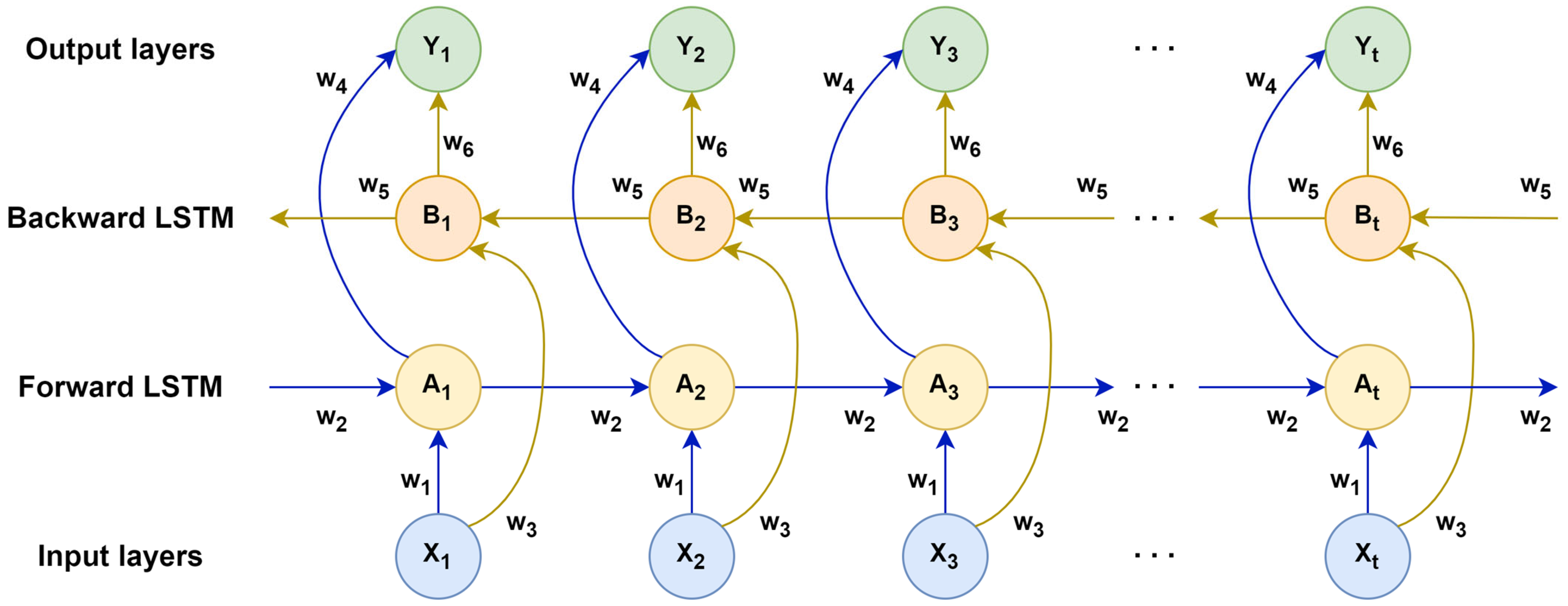
Although LSTMs perform well in addressing long-term dependencies, they can only extract sequential information unidirectionally and cannot simultaneously access information from future time steps in traffic flow prediction. To overcome this limitation, we adopt a bidirectional long short-term memory network (BiLSTM) [44]. By processing input sequences in both forward and backward directions, BiLSTM fully utilizes past and future traffic flow features within time series, thereby capturing complex temporal patterns more comprehensively. This capability enhances the accuracy and stability of model predictions. The structure of BiLSTM is illustrated in Figure 2:

In Figure 2, $X_t$ denotes the traffic flow input data at time step $t$; $A_t$ and $B_t$ represent the corresponding forward and backward iteration LSTM hidden states. ${\mathrm{Y}}_{\mathrm{t}}$ indicates the output result at time step $t$. ${\mathrm{w}}_1~{\mathrm{w}}_6$ denote the respective weights for each layer. The forward LSTM captures historical traffic flow information within the input sequence, while the backward LSTM extracts future traffic flow information. Ultimately, vector concatenation yields a comprehensive hidden layer representation. Thus, the hidden layer at each time step incorporates both forward and backward contextual features. Compared to unidirectional LSTMs, BiLSTMs provide a more comprehensive representation of temporal dependencies, significantly enhancing the model’s prediction accuracy. The state updates for the forward and backward LSTMs, along with the final output process of the BiLSTM, are described by Equations (10)–(12):

$${\mathrm{A}}_{\mathrm{i}}=f_1({\mathrm{w}}_1{x}_i+{\mathrm{w}}_2{\mathrm{A}}_{i-1})$$

(10)

$$B_{\mathrm{i}}=f_2({\mathrm{w}}_3{x}_i+{\mathrm{w}}_5{\mathrm{A}}_{i+1})$$

(11)

$$Y_{\mathrm{i}}=f_3({\mathrm{w}}_4{A}_i+{\mathrm{w}}_6{B}_i)$$

(12)

In the above formula, $f_1$, $f_2$, and $f_3$ represent the activation functions between different layers.

3.5. KAN Model

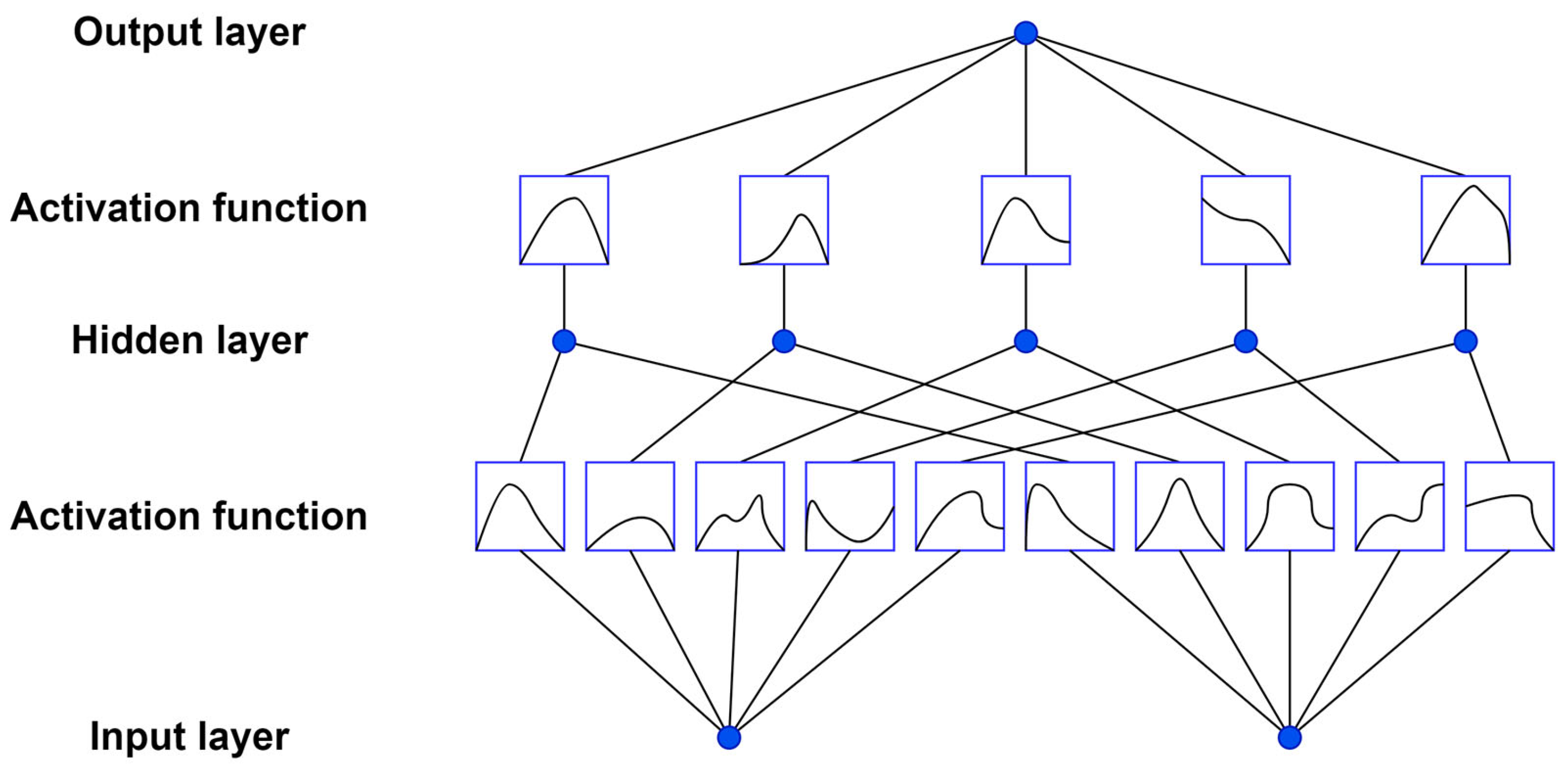
To overcome the limitations of the conventional fully connected network layer in fusing high-dimensional features and modeling complex nonlinear relationships, we replace it with a Kolmogorov–Arnold Network (KAN) [45] to enhance its ability to capture complex nonlinear time-series features. Unlike traditional MLP, which applies activation functions to nodes, KAN applies activation functions to edges, with nodes performing only weighted sum operations. Its core concept involves decomposing high-dimensional nonlinear mappings into combinations of multiple one-dimensional functions. This approach effectively extracts independent features from input variables while establishing global interactions through cross-variable summation mechanisms. Leveraging this mechanism, KAN simultaneously captures both short-term local patterns and long-term dependency features within traffic flow sequences, demonstrating strong generalization performance in complex time series modeling. The network architecture of KAN is illustrated in Figure 3:

In the KAN model, learnable activation functions are placed at the network edges and can adaptively adjust during training. Its network weight parameters are replaced by univariate spline functions, enabling the model to fit complex relationships with fewer parameters while maintaining flexibility. The KAN structure consists of an outer function and an inner function, whose mathematical form is shown in Equation (13):

$$f\left(x\right)=f\left(x_1,\cdots ,x_n\right)=\sum _{q=1}^{2n+1}{\phi }_q\left(\sum _{p=1}^n{\phi }_{q,p}\left(x_p\right)\right)$$

(13)

In the above formula, $\mathrm{x}$ denotes an n-dimensional input vector; ${\mathsf{\phi }}_{\mathrm{q},\mathrm{p}}\left({\mathrm{x}}_{\mathrm{p}}\right)$ represents a learnable activation function, typically with domain $[0,1]$ and range $\mathrm{R}$; ${\mathsf{\phi }}_{\mathrm{q}}$ denotes an external function with both domain and range in $\mathrm{R}$.

To enhance the optimizable of KAN, we introduce a residual activation strategy. Specifically, the learnable activation function $\varnothing \left(x\right)$ is represented as a sum of basis function $b\left(x\right)$ and spline function $spline\left(x\right)$, where the spline functions are parameterized as a linear combination of B-splines. The specific calculation process is shown in Equations (14)–(16):

$$\mathrm{\varnothing }\left(x\right)=w_1·spline\left(x\right)+w_2·b\left(x\right)$$

(14)

$$spline(x)=\sum _{i=1}^n{C}_i{B}_i\left(x\right)$$

(15)

$$b(x)=silu(x)={\displaystyle \frac{x}{1+e^{-x}}}$$

(16)

In the above formula, ${\mathrm{C}}_{\mathrm{i}}$ denotes trainable parameters used to adjust the weights of each spline function; ${\mathrm{B}}_{\mathrm{i}}\left(\mathrm{x}\right)$ denotes the B-spline function used to form the spline combination.

Compared to traditional MLP, KAN features a simpler structure and fewer parameters. By incorporating spline functions, KAN preserves learned information when adapting to new data, thereby avoiding catastrophic forgetting. Simultaneously, it demonstrates superior performance in handling complex nonlinear traffic flow time series. The introduction of KAN not only enhances the model’s ability to capture nonlinear patterns but also improves its generalization capabilities across diverse datasets, thereby further strengthening the model’s functional approximation capabilities.

3.6. KAN-CNN-BiLSTM Model

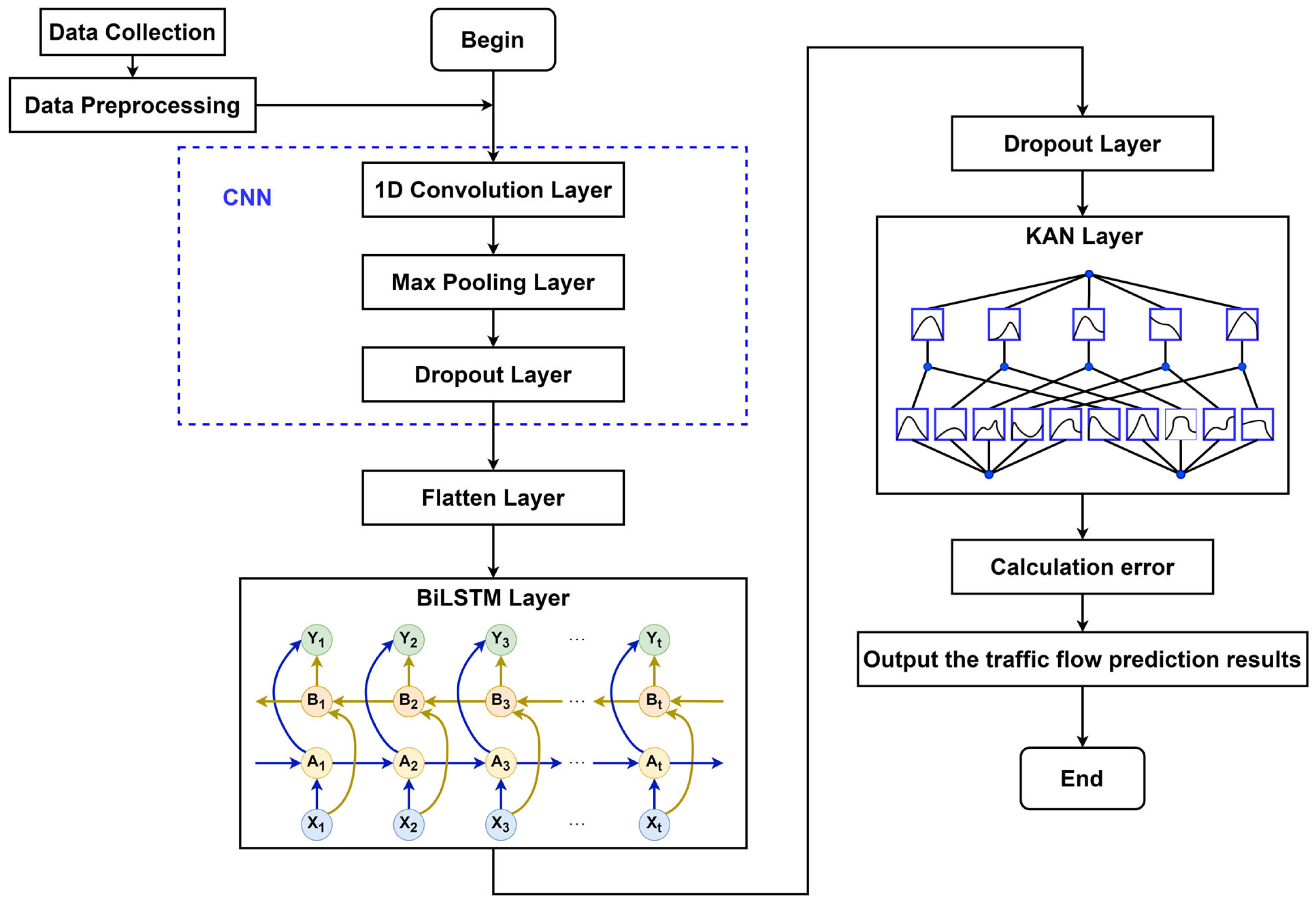
Based on the improvements above, we propose the KAN-CNN-BiLSTM model for short-term traffic flow prediction. In this model, CNN is employed to extract spatial features from traffic flows across different monitoring points, and BiLSTM captures dynamic changes in traffic flow time series. At the same time, the KAN layer, replacing the conventional fully connected layer, enhances the model’s capability for function approximation, thereby improving its fitting accuracy for complex nonlinear relationships in traffic flows. The structure of KAN-CNN-BiLSTM is illustrated in Figure 4:

In the KAN-CNN-BiLSTM model, the preprocessed traffic flow time series data is fed into the model, encompassing both the target road segment and its adjacent segments to fully reflect local traffic dynamics. The input data first enters a one-dimensional (1D) convolutional layer. This layer slides a convolutional kernel over the time series, enabling the extraction of local spatial features and capturing spatial correlations between different road segments. The convolutional output then passes through a max-pooling layer, which reduces feature dimensions, enhances feature robustness, and minimizes noise impact on the model. To prevent overfitting, a Dropout layer is introduced after convolution and pooling to randomly mask some neurons. Next, a Flatten layer transforms the high-dimensional features from convolution and pooling into a one-dimensional vector for input to the BiLSTM. The BiLSTM layer simultaneously processes both forward and backward sequence information, fully capturing the temporal dependency of traffic flow and extracting complex temporal patterns. The BiLSTM output undergoes Dropout layer regularization again to further prevent overfitting. Finally, the output features enter the KAN layer. The KAN layer employs a learnable univariate function combination mechanism to perform nonlinear decomposition and recombination of high-dimensional features. This enhances the model’s ability to represent complex nonlinear characteristics of traffic flow and generates the final short-term traffic flow prediction results.

4. Results

4.1. Experimental Environment and Training Parameters

In terms of experimental environment setup, we divided it into hardware and software components. For hardware, this study employed a 12th-generation Intel Core i9-12900H processor with 16 GB of memory to ensure efficient model training and testing. Regarding software, experiments were conducted on a Windows 10 Professional 64-bit operating system, primarily utilizing MATLAB 2022a to complete all modeling and analysis tasks.

For training parameter settings, we employed a mini-batch gradient descent strategy to optimize network parameters, selecting the Adam algorithm as the optimizer. The model training was set to 100 iterations, with a batch size of 64 for each parameter update and an initial learning rate of ${10}^{-3}$. To capture short-term temporal dependencies, the historical time window length was set to 12. The CNN module consists of stacked one-dimensional convolutional layers (Conv1D) and max pooling layers. The convolutional layer employed 64 kernels of size 2 with a stride of 1. The same padding was applied to maintain consistent spatial dimensions between input and output, while the ReLU activation function enhanced nonlinear feature extraction. The max pooling layer uses a kernel size of 2 with a stride of 1 and same padding to reduce feature dimensions while preserving local key information. The BiLSTM module employed a single-layer bidirectional structure with 512 total hidden units, enabling simultaneous learning of forward and backward dependencies in time series data. To mitigate overfitting, dropout layers with a dropout rate of 0.2 were added after both the CNN and BiLSTM layers, thereby enhancing the model’s generalization capability and training stability.

4.2. Model Evaluation Metrics

In traffic flow prediction tasks, commonly used model performance evaluation metrics include Mean Absolute Error (MAE), Root Mean Square Error (RMSE), and Mean Absolute Percentage Error (MAPE). Lower values of these metrics indicate higher prediction accuracy of the model. MAE measures the average deviation between predicted and actual values, providing an intuitive reflection of the model’s overall prediction accuracy. RMSE reflects the stability of the model’s predictions and quantifies the actual impact of errors. MAPE evaluates the average percentage of prediction errors relative to actual values, revealing the model’s relative error performance across different traffic flow levels. Additionally, to comprehensively evaluate model performance, we introduce the coefficient of determination (R²) as an assessment metric. An R² value closer to 1 indicates better model fit and stronger generalization capability. The calculation formulas for the aforementioned evaluation metrics are as follows:

$$MAE={\displaystyle \frac{1}{n}}\sum _{i=1}^n\left|x_i-\widehat{x_i}\right|$$

(17)

$$RMSE=\sqrt{{\displaystyle \frac{1}{n}}\sum _{i=1}^n{\left(x_i-\widehat{x_i}\right)}^2}$$

(18)

$$MAPE={\displaystyle \frac{100\%}{n}}\sum _{i=1}^n\left|{\displaystyle \frac{x_i-\widehat{x_i}}{x_i}}\right|$$

(19)

$$R^2=1-{\displaystyle \frac{{\sum }_{i=1}^n{\left(\widehat{x_i}-\overline{x}\right)}^2}{{\sum }_{i=1}^n{\left(x_i-\overline{x}\right)}^2}}$$

(20)

In the above formula, $x_i$ represents the actual measured traffic flow value; $\widehat{x_i}$ represents the traffic flow predicted by the model; $\overline{x}$ represents the average traffic flow value; $n$ is the length of the prediction sequence.

4.3. Experimental Results of the KAN-CNN-BiLSTM Model

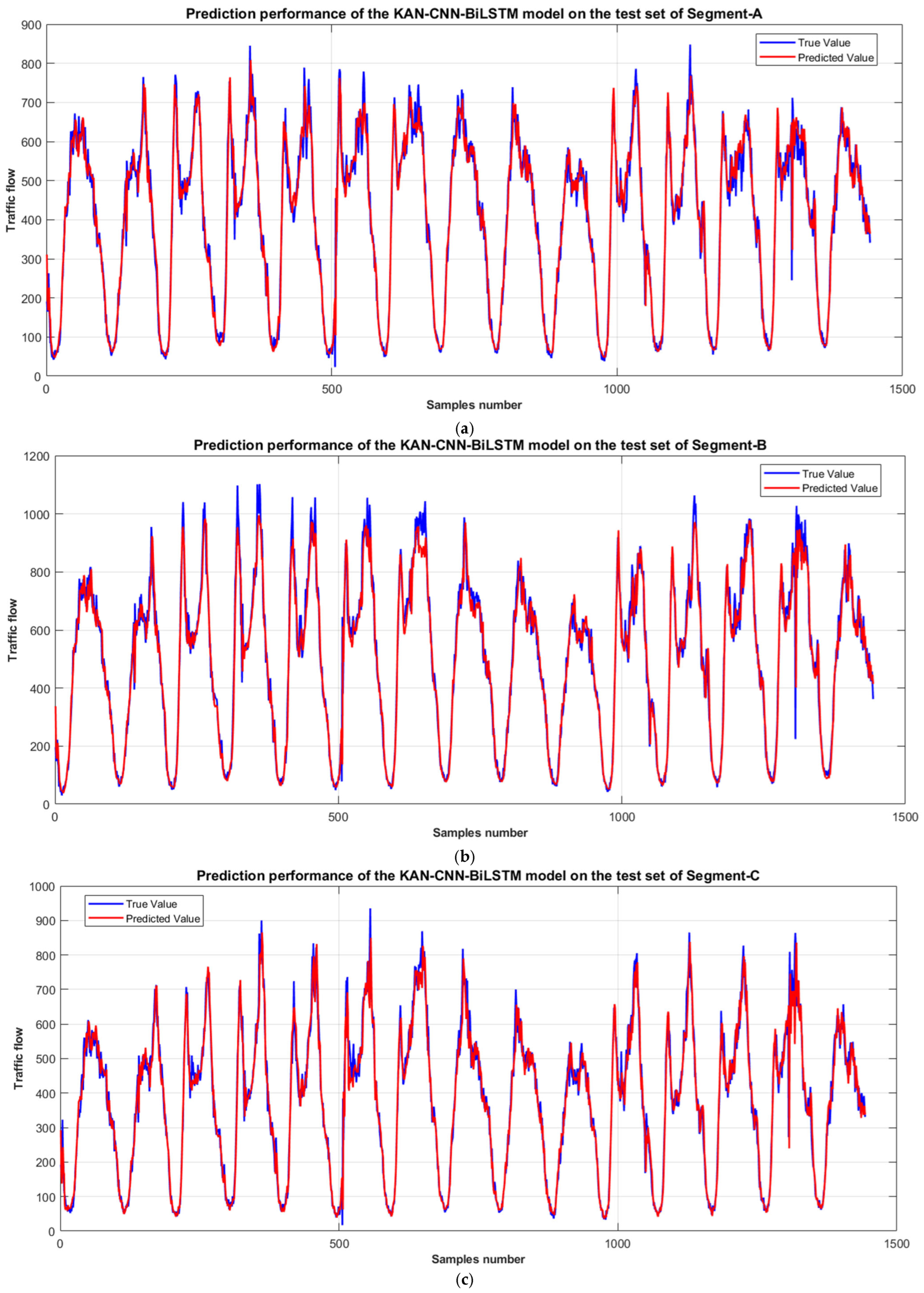
To evaluate the traffic flow prediction performance of the KAN-CNN-BiLSTM model and simultaneously examine the impact of adjacent segment data on the prediction results of the target segment, we designed two sets of experiments. First, the training set traffic flow data from Segment-A, Segment-B, and Segment-C were used as joint inputs for the KAN-CNN-BiLSTM model. The test set from one of these segments was selected as the prediction target to analyze the effect of adjacent segment information on the prediction outcome. The experimental results of the model are shown in

Table 1. Overall experimental results of the KAN-CNN-BiLSTM model integrating the target and adjacent sections.

Dataset	MAE	RMSE	MAPE/%	R2
Segment-A	27.4696	40.3923	8.65	0.9615
Segment-B	36.1295	55.6745	8.63	0.9589
Segment-C	28.9194	43.6814	9.46	0.9566

. Figure 5 visually demonstrates the model’s prediction performance on the test sets of Segment-A, Segment-B, and Segment-C.

To compare the differences between single-segment and multi-segment inputs, we conducted independent experiments using only the data from Segment-A, Segment-B, and Segment-C, respectively, to evaluate the model’s prediction capability in single-segment scenarios. The results of the KAN-CNN-BiLSTM model’s standalone experiments on each dataset are shown in

Table 2. Individual experimental results of the KAN-CNN-BiLSTM model on various datasets.

Dataset	MAE	RMSE	MAPE/%	R2
Segment-A	29.4857	42.7051	9.34	0.9569
Segment-B	36.6609	56.1847	8.87	0.9582
Segment-C	30.7637	44.5591	10.29	0.9547

.

As shown by the experimental results in Table 1 and Table 2, the KAN-CNN-BiLSTM model trained with jointly input data from Segment-A, Segment-B, and Segment-C demonstrates superior performance in short-term traffic flow prediction, exhibiting significant advantages over models trained independently using data from a single segment only. Specifically, the former model achieved average MAE, RMSE, and MAPE values of 30.8395, 46.5827, and 8.91% across the three test datasets, all lower than the latter model’s values of 32.3034, 47.8163, and 9.50%. 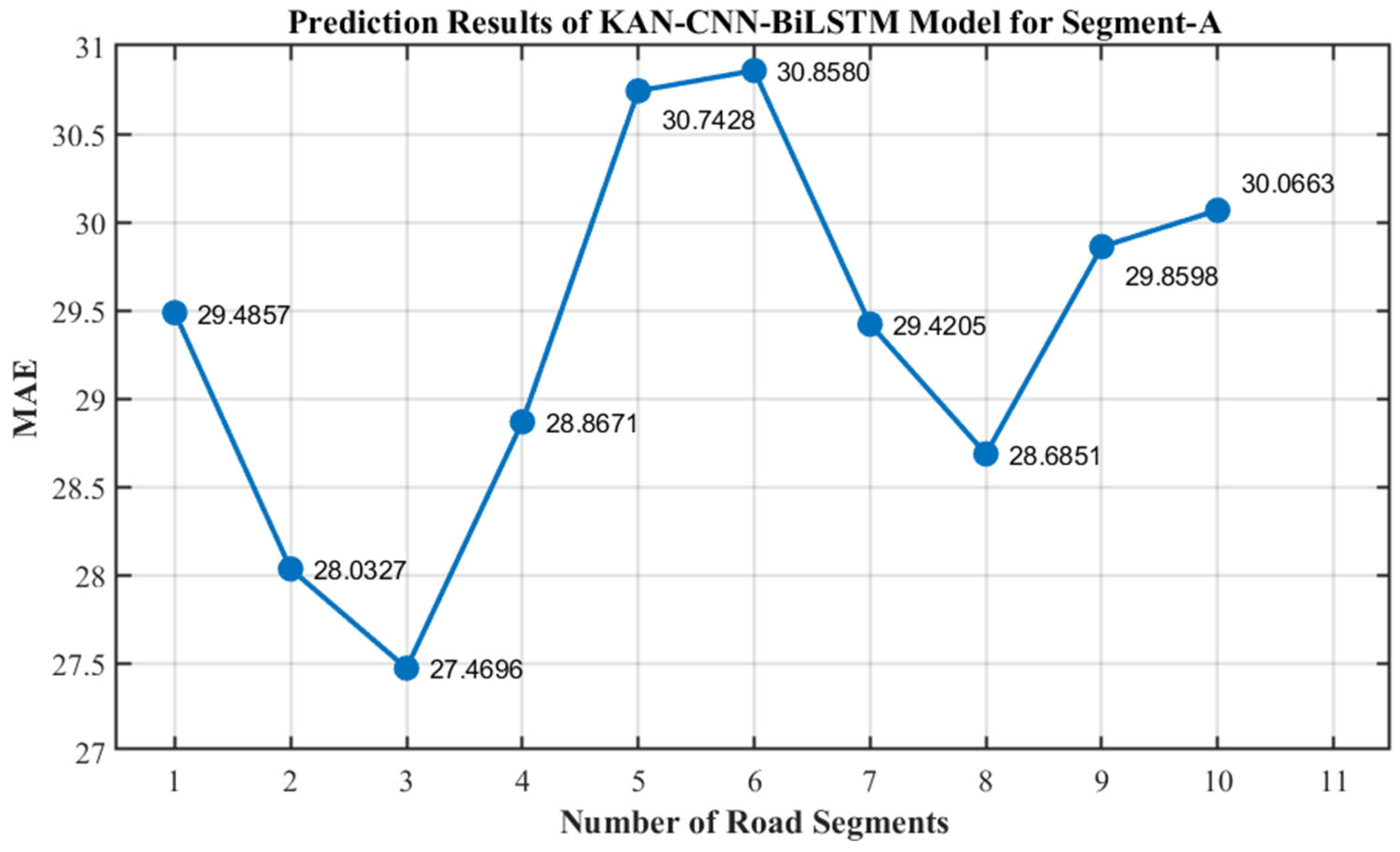Additionally, the former model’s average R² reached 0.959, surpassing the latter model’s 0.9566 and approaching the ideal fitting level. This indicates that the KAN-CNN-BiLSTM model with joint inputs achieves improvements in both prediction accuracy and fitting capability. This further demonstrates the spatial correlation in traffic flow, where incorporating adjacent road segments’ traffic features effectively enhances the model’s overall predictive performance. To evaluate the impact of segment quantity on the predictive performance of the KAN-CNN-BiLSTM model, we conducted experiments using Segment-A as the prediction target. For each experiment, we employed data from 1 to 10 segments adjacent to the target segment as joint input. The corresponding prediction results are shown in Figure 6.

As shown in Figure 6, the MAE of the KAN-CNN-BiLSTM model reaches its minimum when the number of input segments is 3, indicating optimal traffic flow prediction accuracy at this point. As the number of input segments increases, the MAE exhibits noticeable fluctuations and consistently remains above the minimum value, indicating that adding segments does not necessarily enhance prediction performance. Therefore, in subsequent experiments, we selected the Segment-A test set, which exhibited optimal prediction performance, as the target for forecasting. We then combined the training data from Segment-A, Segment-B, and Segment-C as model inputs to fully leverage spatial correlation information. This approach further validated the model’s generalization capability and stability in multi-segment collaborative prediction scenarios.

4.4. Comparative Experiments of Various Models

To validate the reliability and effectiveness of the KAN-CNN-BiLSTM model in short-term traffic flow prediction, this study conducted comparative experiments with several mainstream prediction models. The comparison models included the ARIMA model [9] based on traditional statistical methods, machine learning-based SVM [18], RF [19], and XGBoost model [20], and deep learning-based models including BPNN [28], LSTM [31], GNN [30], CNN-LSTM [46], and PSO-BP model [33]. Furthermore, to further validate the model’s performance in modeling complex spatio-temporal features, we also introduced state-of-the-art models from recent years, including the attention-based CAM-RNN model [47] and AGC-LSTM model [48], as well as the Transformer-based CNN–Transformer model [49].

Table 3. Prediction results of various model on the Segment-A test set.

Model	MAE	RMSE	MAPE/%	R2
ARIMA [9]	41.5203	61.2744	13.67	0.9113
SVM [18]	38.6863	59.0536	11.69	0.9176
RF [19]	37.8854	55.7625	11.76	0.9266
XGBoost [20]	35.1166	54.0243	10.24	0.9311
BPNN [28]	38.0398	58.7892	11.20	0.9184
LSTM [31]	35.7459	53.8240	10.94	0.9316
GNN [30]	36.4528	55.4658	10.99	0.9273
CNN-LSTM [46]	31.7732	44.9431	10.20	0.9523
PSO-BP [33]	29.4724	43.2209	9.33	0.9559
CAM-RNN [47]	34.6983	48.3318	10.83	0.9448
AGC-LSTM [48]	29.7435	43.1173	9.34	0.9562
CNN–Transformer [49]	30.5407	45.6856	9.433	0.9507
KAN-CNN-BiLSTM	27.4696	40.3923	8.65	0.9615

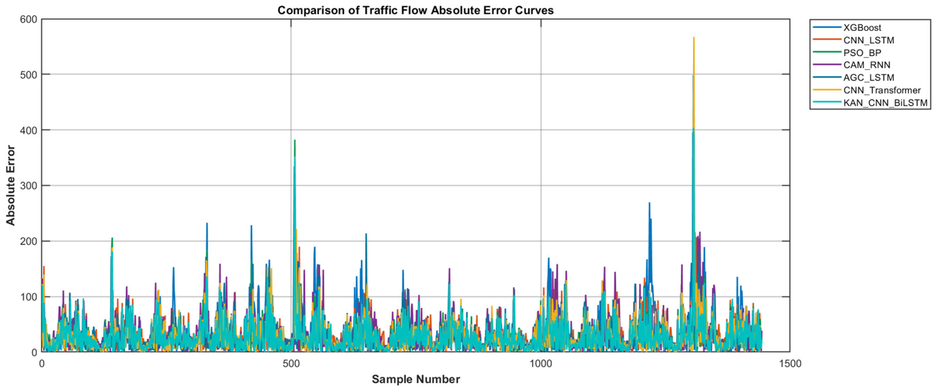
presents the prediction results of each model on the Segment-A test dataset. Figure 7 displays the absolute error curves of seven representative models on the Segment-A test dataset.

As shown in Table 3, the ARIMA model based on traditional statistical methods demonstrates weaker performance in handling nonlinear variations in traffic flow. Its error metrics, which include MAE, RMSE, and MAPE, all exceed those of other models, and its R² value is the lowest, indicating deficiencies in both predictive accuracy and fitting capability. When compared with foundational deep learning models such as BPNN and GNN, the LSTM model achieved the best performance across metrics, including MAE, RMSE, MAPE, and R², demonstrating its strong capability in extracting long-term temporal features and making it suitable for dynamic forecasting of complex traffic flows. Furthermore, the CNN-LSTM model addresses LSTM’s limitation in capturing spatial correlations by incorporating convolutional structures, leading to further reductions in all error metrics and an improved R² value. In recent comparisons of advanced models, the AGC-LSTM model based on the AGC attention mechanism demonstrated the best performance across metrics, including MAE, RMSE, MAPE and R², followed by the CNN-Transformer model. This indicates that attention mechanisms can significantly enhance prediction accuracy by capturing the spatiotemporal characteristics of traffic flow. Among all compared models, our proposed KAN-CNN-BiLSTM model achieved the best results across MAE, RMSE, MAPE, and R², with values of 27.4696, 40.3923, 8.65%, and 0.9615, respectively. This demonstrates the model’s significant advantages in modeling spatio-temporal characteristics and prediction accuracy for traffic flow, enabling it to better handle short-term forecasting tasks in complex traffic environments.

Table 4. Comparison of Training Time and Parameter Count Across Different Models.

Model	Training Time/s	Parameters/104
LSTM [31]	35.33	1.72
Transformer [49]	60.45	7.24
BiLSTM [44]	55.68	4.21
CNN-LSTM [46]	68.49	6.53
CNN-BiLSTM [36]	101.57	9.02
KAN-CNN-BiLSTM	94.91	8.98

lists the training time and parameter count comparisons for representative models. Results show that the LSTM model outperforms the Transformer in training speed and computational overhead, requiring shorter training time and fewer parameters. In contrast, ensemble models generally exhibit longer training times than single models due to their more complex structures and larger parameter counts. Notably, replacing the CNN-BiLSTM’s fully connected network with KAN reduces both training time and parameter count for the KAN-CNN-BiLSTM model. This demonstrates that the KAN architecture is more streamlined, effectively reducing computational burden while maintaining predictive performance.

4.5. Melting Experiment

To further validate the contribution of each component module to the overall performance of the KAN-CNN-BiLSTM model, this study designed four sets of ablation experiments to analyze the impact of different modules on the model’s prediction effectiveness. The specific experimental results are shown in

Table 5. Prediction results of Melting Experiment.

Model	MAE	RMSE	MAPE/%	R2
LSTM [31]	35.7459	53.8240	10.94	0.9316
CNN [29]	41.8035	55.4183	14.61	0.9275
BiLSTM [44]	32.2053	45.0829	10.83	0.9519
CNN-KAN [46]	36.4072	47.8136	13.83	0.9460
CNN-BiLSTM [36]	30.1147	43.9349	9.41	0.9544
KAN-CNN-BiLSTM	27.4696	40.3923	8.65	0.9615

.

In the first set of experiments, to overcome the limitation of traditional LSTM models that can only process time series unidirectionally and fail to fully capture the bidirectional dependencies in traffic flow data, we introduced a bidirectional long short-term memory (BiLSTM) structure to enhance the symmetry extraction capability of time series features. Results indicate that the improved BiLSTM model reduced error metrics such as MAE, RMSE, and MAPE by 3.5406%, 8.7411%, and 0.11%, respectively, while increasing the R² value by 2.2%, thereby enhancing prediction accuracy. In the second set of experiments, we constructed the CNN-KAN model by replacing the traditional fully connected layers in a convolutional neural network (CNN) with a kernel adaptive network (KAN). Experimental results show that compared to the original CNN model, the CNN-KAN model achieved reductions of 5.3963%, 7.6047%, and 0.78% in MAE, RMSE, and MAPE, respectively, while improving the R² metric by 2.0%. In the third set of experiments, we combined CNN with BiLSTM to construct the CNN-BiLSTM model. The CNN component extracts spatial features across different road segment datasets, while the BiLSTM component captures temporal dynamics of traffic flow. Experimental results demonstrate that the CNN-BiLSTM model outperforms both standalone CNN and BiLSTM models across all prediction metrics, validating the effectiveness of integrating spatial and temporal features. In the fourth set of experiments, we introduced a KAN module into the CNN-BiLSTM architecture to further enhance the model’s expressive and approximation capabilities, resulting in the final KAN-CNN-BiLSTM model. Compared to the CNN-BiLSTM model, the KAN-CNN-BiLSTM model reduced MAE, RMSE, and MAPE by 2.6451%, 3.5426%, and 0.76%, respectively, while increasing the R² metric by 0.74%. Overall results demonstrate that integrating the KAN module with the CNN-BiLSTM framework effectively improves the accuracy and stability of traffic flow prediction.

4.6. Generalization Experiment

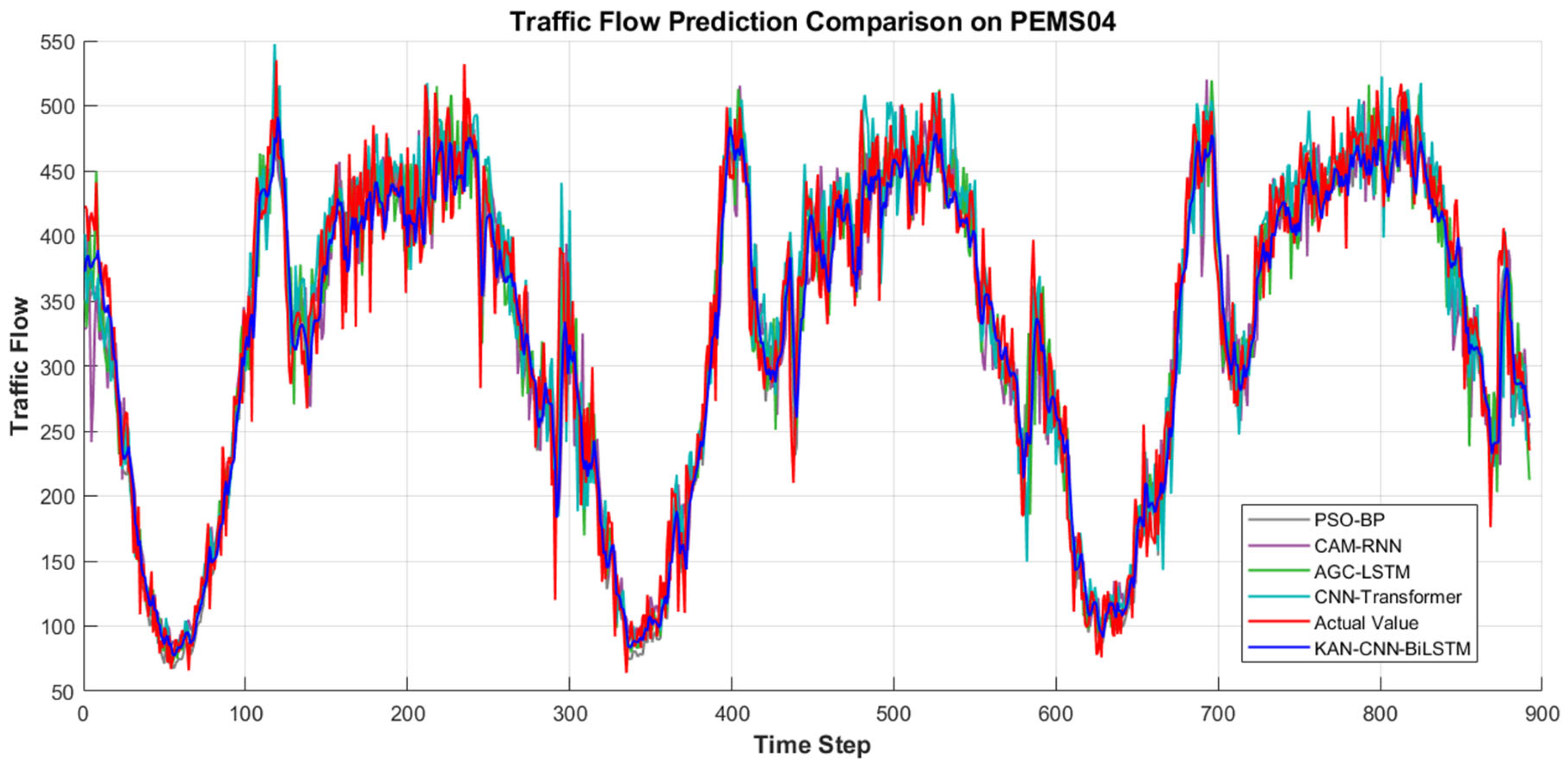
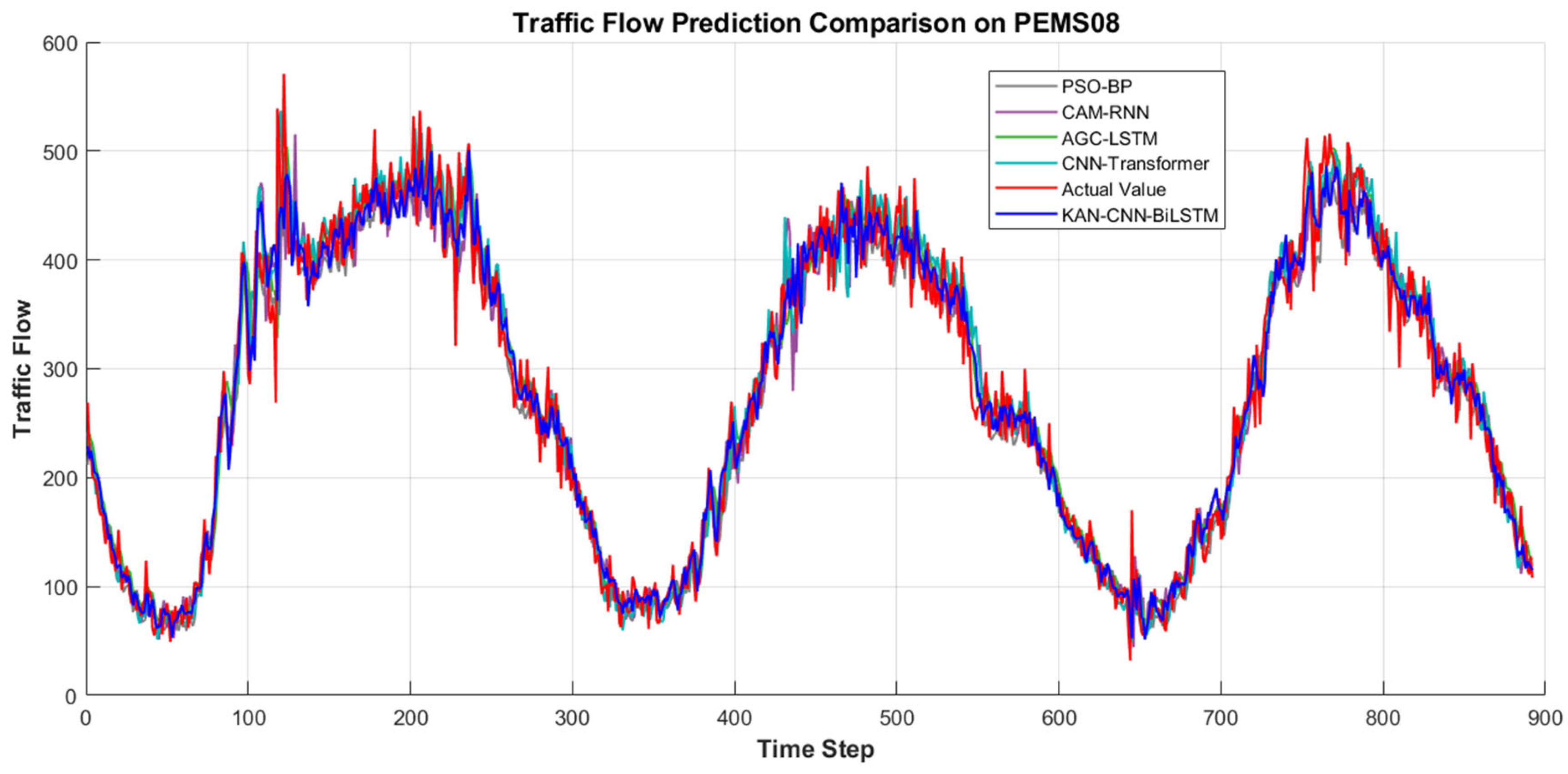
To validate the adaptability and robustness of the KAN-CNN-BiLSTM model across diverse traffic scenarios, this study conducted experiments using several high-performance comparative models, including PSO-BP, CAM-RNN, AGC-LSTM, and CNN–Transformer models. We conducted validation experiments using the PeMS dataset [50] released by the California Department of Transportation (Caltrans), specifically selecting the PEMS04 and PEMS08 sub-datasets. This dataset continuously collects traffic information from highway loop detectors and aggregates it at 5 min intervals, comprehensively reflecting the characteristics of real-world traffic flow variations. For experiments, we selected sections near Sensor 73 in the PEMS04 dataset and Sensor 153 in the PEMS08 dataset, extracting traffic flow data from January 2018. Each dataset contains 8928 records, divided into training, validation, and testing sets at a ratio of 0.8:0.1:0.1. Figure 8 and Figure 9 illustrate the comparison between the prediction results of different models and the actual traffic flow, visually demonstrating the differences in time series fitting among the models.

Table 6. Prediction Results of Five Models on the PEMS04 Dataset.

Model	MAE	RMSE	MAPE/%	R2
PSO-BP [33]	25.7859	33.2920	9.12	0.9264
CAM-RNN [47]	29.6937	39.6162	10.45	0.8959
AGC-LSTM [48]	26.7504	34.9536	9.37	0.9189
CNN–Transformer [49]	28.3018	36.5799	9.81	0.9112
KAN-CNN-BiLSTM	25.4457	33.8102	8.94	0.9287

and

Table 7. Prediction Results of Five Models on the PEMS08 Dataset.

Model	MAE	RMSE	MAPE/%	R2
PSO-BP [33]	21.1239	28.4165	8.96	0.9576
CAM-RNN [47]	22.2892	30.2585	9.71	0.9509
AGC-LSTM [48]	20.5308	27.6593	9.20	0.9589
CNN–Transformer [49]	21.5039	28.7755	9.28	0.9556
KAN-CNN-BiLSTM	19.7301	26.8879	8.47	0.9612

present the results of each model on the PEMS04 and PEMS08 datasets.

In the traffic flow prediction experiment using the PEMS04 dataset, the KAN-CNN-BiLSTM model achieved optimal results across all metrics: MAE of 25.4457, MAPE of 8.94%, and R² of 0.9287. In experiments on the PEMS08 dataset, this model also demonstrated superior performance, achieving MAE, RMSE, MAPE, and R² values of 19.7301, 26.8879, 8.47%, and 0.9612, respectively. The comprehensive experimental results demonstrate that the KAN-CNN-BiLSTM model exhibits high prediction accuracy and good adaptability across different traffic datasets, effectively capturing the dynamic characteristics of traffic flow.

5. Discussion

We conducted experiments using traffic flow data from three adjacent sections of the M4 motorway near London Heathrow Airport. Results indicate significant spatial correlations in traffic flow, where traffic characteristics from neighboring sections positively influence predictions for the target section. Incorporating spatial features from adjacent sections during model training significantly improved overall prediction performance. In comparative experiments against various mainstream machine learning and deep learning models, our proposed KAN-CNN-BiLSTM model achieved the best performance across all evaluation metrics. Specifically, the model attained MAE, RMSE, MAPE, and R² values of 27.4696, 40.3923, 8.65%, and 0.9615, respectively, outperforming all other models. The results demonstrate that the KAN-CNN-BiLSTM model possesses outstanding comprehensive advantages in capturing the spatio-temporal characteristics of traffic flow and enhancing short-term prediction accuracy. It can more effectively address dynamic changes in complex traffic environments and better handle short-term prediction tasks under such conditions.

Although the proposed KAN-CNN-BiLSTM model outperforms several mainstream machine learning and deep learning models in traffic flow prediction, it still has some limitations. First, the model’s prediction error remains relatively high, primarily due to the presence of outliers in the dataset caused by traffic accidents, which the current model cannot effectively identify and respond to. Second, weather factors significantly impact traffic flow [5]. Extreme weather conditions (such as heavy rain or snow) often significantly alter people’s travel behavior. However, due to data limitations, this study was unable to obtain real-time meteorological data for the corresponding time periods, thereby restricting the model’s adaptability in this regard. Finally, the experiments in this study were conducted solely based on traffic data from the M4 motorway near London Heathrow Airport, and the model’s transferability and universality have not been fully validated. To further evaluate generalization, we conducted validation experiments using the PeMS dataset released by the California Department of Transportation (Caltrans), specifically selecting the PEMS04 and PEMS08 sub-datasets. Future research will focus on incorporating multi-source heterogeneous data (including real-time meteorological and traffic incident information) to enhance the model’s sensitivity and robustness to anomalies. Concurrently, we will validate the model’s generalization capabilities across diverse regions and road types to elevate its applicability in complex traffic scenarios.

6. Conclusions

To address the limitations of traditional traffic flow prediction models in spatial feature extraction, time-dependent modeling, and nonlinear relationship representation, we propose the KAN-CNN-BiLSTM model to enhance the accuracy and stability of short-term road traffic flow prediction. First, to overcome the limitations of previous studies that overly relied on data from a single road segment while neglecting spatial correlations, the model simultaneously incorporates traffic flow information from the target segment and its two adjacent segments into the input layer. This approach provides a more comprehensive reflection of local traffic conditions and reduces biases introduced by single-segment features. Second, to address LSTM’s weakness in spatial feature extraction, the model incorporates a Convolutional Neural Network (CNN) to capture spatial correlations between monitoring points. Combined with LSTM’s temporal modeling capabilities, this enables joint spatio-temporal feature learning for traffic flow, enhancing the model’s adaptability to dynamic changes. Third, addressing LSTM’s limitation of processing time series unidirectionally and its difficulty in simultaneously utilizing historical and future information, the model employs a bidirectional long short-term memory network (BiLSTM). By integrating forward and backward information, it more comprehensively captures the time-dependent characteristics of traffic flow. Finally, to further enhance the model’s nonlinear representation and information fusion capabilities in high-dimensional traffic data, the Kolmogorov–Arnold network (KAN) replaces the traditional fully connected layer. The KAN enhances the model’s functional approximation capabilities through its learnable function mapping mechanism, thereby effectively improving prediction accuracy and generalization performance. In experiments, KAN-CNN-BiLSTM demonstrated significantly superior prediction performance compared to all benchmark models on the UK Highways Agency traffic flow dataset, achieving a Mean Absolute Error (MAE) of 27.4696, Root Mean Square Error (RMSE) of 40.3923, Mean Absolute Percentage Error (MAPE) of 8.65%, and an R² value of 0.9615. These metrics clearly demonstrate that KAN-CNN-BiLSTM possesses significant advantages in capturing spatio-temporal features of traffic flow and achieving high short-term prediction accuracy. It provides an efficient and robust solution for short-term traffic flow forecasting in complex traffic environments.