Low-Carbon Water Ecological POI Logistics Route Planning Based on Improved Water Network Space AGNES Clustering Model and Symmetrical Simulated Huffman Spatial Searching Tree Algorithm

Abstract

To reduce the pollutant emissions of water ecological POI logistics, the water ecological POI logistics route-planning method based on the improved water network space AGNES clustering model and the symmetrical simulated Huffman spatial searching tree (SHSST) algorithm is innovatively established. The improved AGNES algorithm is established for water ecological POI clustering, and then the logistics distribution center location model based on water ecological POI clustering is constructed. On the basis of an optimal distribution center, combining the symmetrical feature of vehicle moving paths and distances in logistics sub-intervals and logistics intervals, the sub-interval optimal route-searching algorithm based on the symmetrical SHSST is constructed to determine the optimal path for each logistics sub-interval, and then the global logistics route-planning algorithm based on undirected complete graph spatial search is constructed to search for the global optimal logistics route. Experiments prove that the proposed algorithm can accurately cluster water ecological POIs and output the logistics route with the lowest costs and pollutant emissions. Compared to the traditional AGNES and other clustering algorithms, the improved AGNES algorithm has lower time complexity. Compared to the traditional logistics route algorithms, SHSST has lower algorithm complexity, route costs, and pollutant emissions, and strong stability. The minimum and maximum optimization rates for the same route are 10.06% and 17.58%, while the minimum and maximum optimization rates for the optimal route are 11.41% and 14.29%; it could effectively reduce the negative impact of pollutants on the water ecological environment and POIs.

1. Introduction

1.1. Research Background

Providing comprehensive and thoughtful material support for tourists is an important part of the construction of smart tourism and tourism logistics systems. Tourists will generate a large amount of material consumption, such as dining, shopping, etc. [1], when acting within the point of interest (POI) in a city. These consumption activities are highly dependent on materials and require a continuous supply of goods, especially during the peak tourism season, when a large influx of tourists into POIs can generate consumption beyond the normal load range. This requires the urban material distribution system to have complete replenishment capabilities and efficient replenishment efficiency [2]. When multiple POIs in a city require material replenishment, the transportation process of material distribution vehicles from the departure point to multiple POIs will form a complete route, and produce time costs, distance costs, and energy consumption, emitting harmful gases such as carbon monoxide, hydrocarbons, nitrogen oxides, etc. Therefore, in cities with water ecology as the main tourism environment and destination, the protection of the water ecological environment and the control of pollutant emissions are very important. It is necessary to minimize the pollutant emissions and reduce their damage to the water ecological environment as much as possible [3]. From the perspective of protecting the water ecological environment and satisfying the efficient distribution of materials during the peak tourism season, POI logistics route planning should be optimized from the following aspects. Firstly, when the material distribution vehicles depart from the distribution center to deliver materials to multiple POIs that have been determined, the selection of the starting point is crucial. It is the primary condition for reducing energy consumption and harmful emissions; that is, a spatial relationship should be established between the distribution center and the POIs. On the basis of constructing the spatial relationship model between the distribution center and the POIs, determine the optimal distribution center as the starting point. Secondly, in order to realize the efficient supply of POI materials, it is necessary to reduce the time and distance costs of transportation, ensuring that the closed route formed by vehicles departing from the distribution center and returning to the distribution center after delivery to all POIs produces the lowest transportation time and distance. Thirdly, when the material distribution vehicles pass between nodes composed of distribution centers and POIs, the algorithm needs to be constructed to optimize the internal node pathway, minimizing the time cost, distance cost, energy consumption, and pollutant emissions of sub-intervals. When the cost of the sub-interval is the lowest, it can minimize the cost of the entire distribution route [4]. The above three factors, constructing the spatial relationship model between distribution centers and POIs, selecting the optimal starting point based on the POIs that require delivery, and constructing the sub-interval and the global optimal material distribution route models, are effective ways to control the distribution costs, reduce the energy consumption, and minimize the pollutant emissions, which can reduce the damage of tourism logistics to the water resources and the water environment.

1.2. Existing Problems

Tourism destinations with water ecology as the main body, including urban rivers, lakes, wetland parks, springs, reservoirs, and other tourism POIs, are different from the cultural and historical POIs in that they have ecological attributes, natural attributes, and could be easily destroyed. Their ecological attributes are fragile and susceptible to external factors such as sewage, exhaust gas, and acid rain, and are difficult to repair. Among multiple factors, the air pollution and the resulting disasters, such as acid rain, not only cause damage to water bodies, but also have a certain impact on the ecosystems where water bodies are located [5]. In cities, the tourism logistics system covers a huge volume of transportation. During peak tourism seasons, multiple logistics companies may have multiple vehicles transporting materials for POIs. When calculated on an annual basis, all logistics vehicles in a large city can generate tens of thousands of tons of exhaust pollutants per year. To address this issue, the mainstream solutions for the automobile pollutant emissions include the following: Optimizing the engines, improving the fuel efficiency, and reducing harmful emissions; adopting environmentally friendly and energy-saving modes of transportation as much as possible, and increasing the utilization rate of public transportation; and improving the efficiency of vehicle usage and optimizing the transportation routes [6]. The mainstream solutions for optimizing logistics routes currently include the following: firstly, optimizing the logistics routes to reduce transportation distance and costs. At present, operations research algorithms, graph theory algorithms, and shortest path algorithms are mainly used to design routes. Traditional methods have low computational complexity and feasibility when there are fewer route nodes. However, when there are more POIs and more sub-interval road nodes, the traditional optimization algorithms will have huge computational complexity and inherent defects, making it difficult to output the global optimal solution. Secondly, using autonomous vehicles for delivery can reduce labor costs and energy consumption. It introduces intelligent vehicles but only optimizes from the perspective of intelligent recognition and reducing labor costs, without solving the problem from the perspective of energy conservation and reducing exhaust emissions, which has certain shortcomings. Thirdly, there is a lack of in-depth research on the spatial relationship between distribution centers and POIs, resulting in strong randomness in the selection of logistics route departure points and unscientific determination of delivery sequences. This leads to logistics routes that connect multiple POIs not being globally optimal, making it difficult to truly reduce the energy consumption and costs, or reduce the pollutant emissions.

2. Literature Review

2.1. Related Works and Analysis

Regarding the optimization of logistics routes, numerous scholars have conducted extensive research, and we selected representative studies for analysis. Zhang et al. [7] focused on the optimization problem regarding the vehicle routing problem (VRP) in supermarket store delivery, using chain supermarkets as the research objects. A path optimization algorithm was constructed by integrating the Floyd algorithm, the nearest neighbor algorithm, and the insertion algorithm, effectively reducing the carbon emissions in the logistics process. Da et al. [8] designed a logistics planning system based on the Baidu Maps development package, which achieved enterprise logistics planning and tracking. This study utilized the development package provided by Baidu Maps, combined with map and geospatial data, to integrate logistics planning at the level of Baidu Maps, which improves the efficiency of logistics planning. Zhang [9] developed a factory-end logistics distribution path optimization method based on the k-means clustering to address the problems of scattered logistics data and low logistics distribution efficiency in existing methods for factory-end logistics distribution path planning. This study optimized the k-means clustering algorithm and used it to collect the logistics distribution data at the factory end. It established the priority features of the logistics distribution nodes and a subset of distribution service requirements and designed the end distribution path planning process to achieve route optimization for factory-end logistics distribution. Puspitasari et al. [10] used the classical vehicle routing problem (VRP) mathematical model to determine the material distribution route with the goal of minimizing travel time. This study designed a dedicated area for each delivery person and used delivery person allocation optimization to minimize mileage. Febriandini et al. [11] used the VRP to find the optimal distribution route for gasoline products, taking into account the demand for the gasoline products, tank truck capacity, distribution costs, and number of cabins. They developed a mathematical expression for MC-VRP in a mixed-integer linear programming (MILP) model. Using the Ilog Cplex algorithm with branch and bound, the gasoline delivery problem is solved with the minimum total delivery cost. Kleinová et al. [12] studied the application of the latest generative artificial intelligence, ChatGPT-3.5, in material distribution route planning, using ChatGPT-3.5 to optimize distribution routes, which significantly reduced the total travel distance and greatly saved the transportation costs. Sembiring et al. [13] conducted research on optimizing the product distribution routes to minimize distribution costs. The study used the traveling salesman problem (TSP) method, which combined several of the nearest delivery routes and improved the route sequence, and then developed sub-routes formed by travel time and the utility of the transportation equipment efficiency, generating the minimum mileage on each sub-route and ultimately shortening the transportation mileage and time. Ma et al. [14] aimed to minimize transportation and time costs and established a model with constraints on the number of trucks, load quality, load capacity, maximum distance, and customer service time. They used the Floyd algorithm to determine the movement path with road constraints and the shortest distance between each point. Based on the operational requirements of picking goods, time costs, transportation costs, and other factors, they determined the order of delivery and pickup points as well as the delivery route. Adam et al. [15] used the nearest neighbor method to design a path based on the next nearest distance and evaluated the delivery efficiency based on the total distance, time, and load borne by the fleet, which effectively saved the transportation costs and expenses of the delivery company. Wang et al. [16] studied the planning and selection problem of a cold chain item delivery path optimization model with variable customer demands and established a cold chain logistics delivery model with the goal of minimizing the total delivery cost. The optimal paths planned by the random distribution model (considering changes in customer demands) and the deterministic distribution model (based on given demand expectations) were compared through numerical examples. The total delivery cost obtained by the two models increased with the degree of demand change. Bukhari et al. [17] proposed a sustainable green supply chain and logistics network using an adaptive fuzzy particle swarm optimization (AFPSO) method, which evaluated performance using parameters such as energy consumption, implementation cost, error values, and activation procedures. Compared with traditional optimization methods, the constructed method has higher energy efficiency, lower cost, higher accuracy, and better stability. Gu [18] proposed an improvement strategy for the shark optimization algorithm in group optimization algorithms to enhance its convergence speed and global search ability in solving logistics path optimization problems, while maintaining algorithm stability and improving its adaptability and flexibility. Gan [19] studied the construction of the vehicle routing problem model with a time frame. A hybrid optimization algorithm based on the fish swarm algorithm and the ant colony algorithm is proposed for optimizing delivery routes. The hybrid optimization algorithm compensates for the shortcomings of independent algorithms and improves the performance of the algorithm to a certain extent. Liu et al. [20] proposed an attention-enhanced deep reinforcement logistics network that integrates attention mechanisms to optimize route planning for autonomous delivery fleets. This model combines an improved reward and state transition function, which can effectively learn the optimal path strategy and achieve stable path optimization.

Based on the analysis of the aforementioned studies, it can be concluded that current research on logistics route planning mainly focuses on urban logistics or intercity logistics. There are still some problems in the research objectives and methods of existing studies. Firstly, the research objective is mostly to reduce the transportation costs of logistics companies, rather than to protect the water ecological environment, water resources, etc. Through analyzing the large body of literature, we acknowledge that there is currently a significant lack of literature aimed at protecting the urban water ecological environment. Secondly, most studies use the traditional operations research methods, shortest path searching algorithms, etc., to plan logistics routes. However, the operations research algorithms and shortest path searching algorithms themselves have certain drawbacks, and most experiments verify the models through simulation examples, making the research theoretically feasible. However, due to the lack of research in real environments, their feasibility verification in specific practical applications is insufficient. Some research applied artificial intelligence algorithms, such as swarm intelligence optimization and reinforcement learning, to optimize logistics routes. However, these methods have shortcomings such as complex algorithm logic, high time complexity, susceptibility to premature convergence, and a high dependence on parameters. Thirdly, most studies do not consider the spatial relationship between distribution centers and POIs during modeling, and do not establish a spatial relationship model between the two factors, resulting in the blind selection of route departure points. When there are many available distribution centers, choosing the optimal distribution center is the key to determining the optimal logistics route. Fourthly, the complexity of POI distribution, road network distribution, and road node distribution in cities is high, and the traditional optimization algorithms are prone to increasing the computational complexity and inability to search for optimal solutions when the number of nodes increases. Therefore, it is necessary to design intelligent optimization algorithms that combine geospatial constraints to search for the optimal solution of each logistics sub-interval in order to obtain the global optimal solution.

2.2. The Proposed Solution

In response to the research background and existing research problems, we studied several problems in water ecological tourism logistics route planning from the perspective of urban water ecological tourism. We constructed the low-carbon water ecological POI logistics route-planning algorithm based on the improved water network space AGNES clustering model and the symmetrical simulated Huffman spatial searching tree algorithm. From the perspective of protecting the water ecological environment, the improved water network space AGNES clustering model is designed to establish water ecological POI clustering within the buffer zone of the water network, which could explore the geospatial distribution patterns of water ecological POIs [21,22]. Secondly, we determined the specific locations of the urban distribution centers and constructed a spatial relationship model between distribution centers and clusters, as well as with the water ecological POIs. By analyzing the quantity and locations of water ecological POIs to be delivered, we searched for the starting and ending points of tourism logistics routes. Finally, after determining the starting point of the logistics route, the water ecological POIs to be delivered, and the endpoint of the logistics route, the symmetrical logistics route sub-interval and logistics route interval are constructed, and then the multi-level symmetrical simulated Huffman spatial searching tree algorithm is established to search for the optimal route in each sub-interval, iteratively outputting the global optimal route for water ecological logistics.

The objectives and motivations of our proposed algorithm are as follows: Firstly, to achieve closeness clustering between water ecological POIs and river water networks, which constrains the locations of distribution points within the spatial buffer zones of POI clusters, gathers POIs to great extent, and, finally, reduces the spatial distances between distribution points and POIs, improving the logistics transportation efficiency and reducing the energy consumption and pollutant emissions. Secondly, to search for the optimal logistics route to minimize the distance of a transportation route when delivering materials to the same POIs, reducing the energy consumption and pollutant emissions. Based on the unit vehicle and single transportation task, the pollutant emission in a single transportation task is better than traditional route algorithms. When the number of logistics times, vehicles, working hours, etc., shows a large-scale trend, the proposed algorithm can greatly reduce the pollutant emissions, improve the energy utilization efficiency, and achieve sustainable and efficient water ecological environment protection.

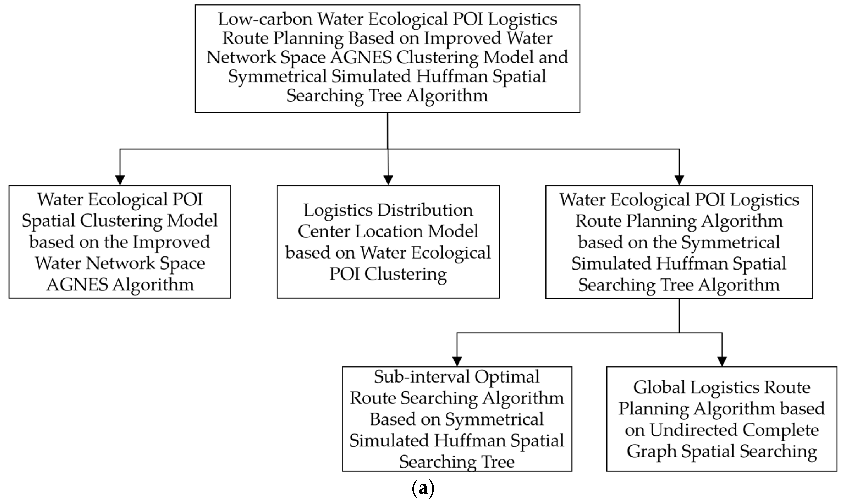
The specific solutions and contributions of the work are as follows. Figure 1 shows the main content, structure, and logical relationships between the proposed algorithms in the work. Figure 1a shows the main content and structure of the work, and Figure 1b shows the logical relationships between the proposed improved AGNES clustering, the simulated Huffman spatial searching tree algorithm, and the logistics route algorithm.

Firstly, the water ecological POI spatial clustering model based on the improved water network space AGNES algorithm is constructed. In cities with water ecological tourism as the main body and intersecting river networks, we construct the spatial distribution model of the main water network and determine the matrix of water network control points. By constructing an improved AGNES clustering algorithm and building the clustering relationship model between the water ecological POIs and water network buffer zones, a spatial cluster is formed within the water network buffer zone to quantify the spatial relationship of POIs.

Secondly, the logistics distribution center location model based on the water ecological POI clustering is established, which is a spatial relationship model between the urban distribution centers and water ecological POIs in each cluster. By searching for the spatial relationship and the number of subordinates between the distribution center and the POI cluster, we determined the POI cluster that is used to select the logistics departure point, and then searched for the optimal distribution center location within the cluster. It can control the total cost of logistics routes and reduce the pollutant emissions of logistics vehicles from the perspective of the optimal location of distribution centers.

Thirdly, the water ecological POI logistics route-planning algorithm based on the symmetrical simulated Huffman spatial searching tree algorithm is established. Using the logistics distribution centers and water ecological POIs to be delivered as nodes in a simulated Huffman spatial searching tree, a multi-level symmetrical simulated Huffman spatial searching tree is established within the logistics sub-intervals and logistics intervals. The optimal routes for the sub-intervals and intervals are searched separately to obtain the global optimal solution, minimizing the logistics costs and pollutant emissions.

3. Methodology

In response to the spatial distribution features of the water ecological POIs and the demands for the logistics route planning, we first construct the clustering relationship model between the water ecological POIs and the water network buffer zones. Secondly, we establish the spatial relationship model between the urban distribution centers and water ecological POIs in each cluster, and search for the optimal distribution center location as the starting and ending points of logistics routes. Based on this, we construct a multi-level logistics route algorithm based on the symmetrical simulated Huffman spatial searching tree algorithm to search for the optimal routes in the logistics sub-intervals and logistics intervals.

3.1. Water Ecological POI Spatial Clustering Model Based on Improved Water Network Space AGNES Algorithm

Water ecological POIs are distributed in urban geospatial environments and have geographic spatial attributes such as geographic coordinates, spatial distance, etc. In tourist cities dominated by water ecological POIs and water network rivers, the water network rivers form the natural network system and are usually represented by linear symbols on maps [23,24]. For the water network rivers represented by linear symbols, we selected those with important tourism value and basic water ecological architecture from the urban geospatial environment, and projected them onto the coordinate system to form the meta-structure of water ecological POI clustering. By establishing the urban spatial road network, we constructed the control point set for the main water network meta-structure, and then used the control point set to construct a buffer zone for the main water network meta-structure. Then, the improved AGNES clustering algorithm was established to achieve the spatial relationship between the water ecological POIs and control point set, thereby realizing the water ecological POI clustering based on the main water network meta-structure.

Definition 1. 

Establish a coordinate system covering all water ecological POIs and water network in the water tourism city. The coordinate system is defined as the water ecological POI clustering coordinate system, denoted as $xoy$. The water ecological POI for material distribution is defined as a water ecological POI element. If the number of element $P_{(i)}$ in the city is $N$, then $0<i\le N$, $i,N\in N$. The geographic coordinates of $P_{(i)}$ in $xoy$ are denoted as $x_{P_{(i)}}$ and $y_{P_{(i)}}$.

Definition 2. 

The selected main roads in the water tourism city are projected onto $xoy$ to form a road network, denoted as ${NET}_{Ro}$. The selected main water network channels in the water tourism city are projected onto $xoy$ to form the main water network meta-structure, denoted as $WMS$. Project $WMS$ onto $xoy$ and extract $m$ number of rivers, and each river is denoted as a dataset element $W_{(i)}$, $0<i\le m$, $i,m\in N$. The dataset $W$ consisting of the $m$ number of extracted rivers $W_{(i)}$ is defined as the $WMS$ river projection dataset. The $W$ is a subset of $WMS$.

Definition 3. 

The water ecological POI buffer zone is formed by the  $W_{(i)}$, which is extended to form the POI cluster $C_{(i)}$, $0<i\le m$, $i,m\in N$, where $m$ is the number of the clusters. The point set formed by the intersection of element $\forall W_{(i)}$ and the ${NET}_{Ro}$ is defined as the cluster control point set, denoted as $C_{on(i)}$. Set the number of control points in $C_{on(i)}$ of $C_{(i)}$ as $t_{(i)}$, and the $t_{(i)}$ number of control points form the structure of $C_{on(i)}$, $C_{(i)}$ and $W_{(i)}$. Note the element of $C_{on(i)}$ as $C_{on(i,j)}$, as No. $j$ control point of $C_{on(i)}$, $0<j\le t_{(i)}$, $j,t_{(i)}\in N$. The coordinates of $C_{on(i,j)}$ are $x_{C_{on(i,j)}}$ and $y_{C_{on(i,j)}}$.

Definition 4. 

Construct a  $m\times \max t_{(i)}$ dimension matrix ${\mathbf{M}}_{\mathrm{C}on}$ to store the set $C_{on(i)}$ of control points in $W_{(i)}$ of the dataset $W$. The rows represent the elements $W_{(i)}~C_{(i)}$ and the columns represent the No. $j$ control point $C_{on(i,j)}$. When the $N$ number of water ecological POIs form $m$ number of clusters $W_{(i)}~C_{(i)}$, a $m\times \max N_{(i)}$ dimension matrix $C$ is constructed to store each cluster POI. The rows represent clusters $W_{(i)}~C_{(i)}$ and the columns represent the No. $j$ POI element $P_{(i)}~C_{(i,j)}$ of the cluster, $0<j\le N_{(i)}$, $j,N_{(i)}\in N$. Formulas (1) and (2) represent the matrix ${\mathbf{M}}_{\mathbf{C}on}$, and Formula (3) is the matrix $C$.

$${\mathbf{M}}_{\mathrm{C}on}={\left[{C_{on(1)}}^T,{C_{on(2)}}^T,\dots ,{C_{on(i)}}^T,\dots {C_{on(m)}}^T\right]}^T$$

(1)

$${\mathbf{M}}_{\mathrm{C}on}=\left[\begin{array}{cccccc}{C}_{on(1,1)}& C_{on(1,2)}& \dots & C_{on(1,j)}& \dots & C_{on(1,t_{(1)})}\\ C_{on(2,1)}& C_{on(2,2)}& \dots & C_{on(2,j)}& \dots & C_{on(2,t_{(2)})}\\ \dots & \dots & \dots & \dots & \dots & \dots \\ C_{on(i,1)}& C_{on(i,2)}& \dots & C_{on(i,j)}& \dots & C_{on(i,t_{(i)})}\\ \dots & \dots & \dots & \dots & \dots & \dots \\ C_{on(m,1)}& C_{on(m,2)}& \dots & C_{on(m,j)}& \dots & C_{on(m,t_{(m)})}\end{array}\right]$$

(2)

$$C=\left[\begin{array}{cccccc}{C}_{(1,1)}& C_{(1,2)}& \dots & C_{(1,j)}& \dots & C_{(1,N_{(1)})}\\ C_{(2,1)}& C_{(2,2)}& \dots & C_{(2,j)}& \dots & C_{(2,N_{(2)})}\\ \dots & \dots & \dots & \dots & \dots & \dots \\ C_{(i,1)}& C_{(i,2)}& \dots & C_{(i,j)}& \dots & C_{(i,N_{(i)})}\\ \dots & \dots & \dots & \dots & \dots & \dots \\ C_{(m,1)}& C_{(m,2)}& \dots & C_{(m,j)}& \dots & C_{(m,N_{(m)})}\end{array}\right]$$

(3)

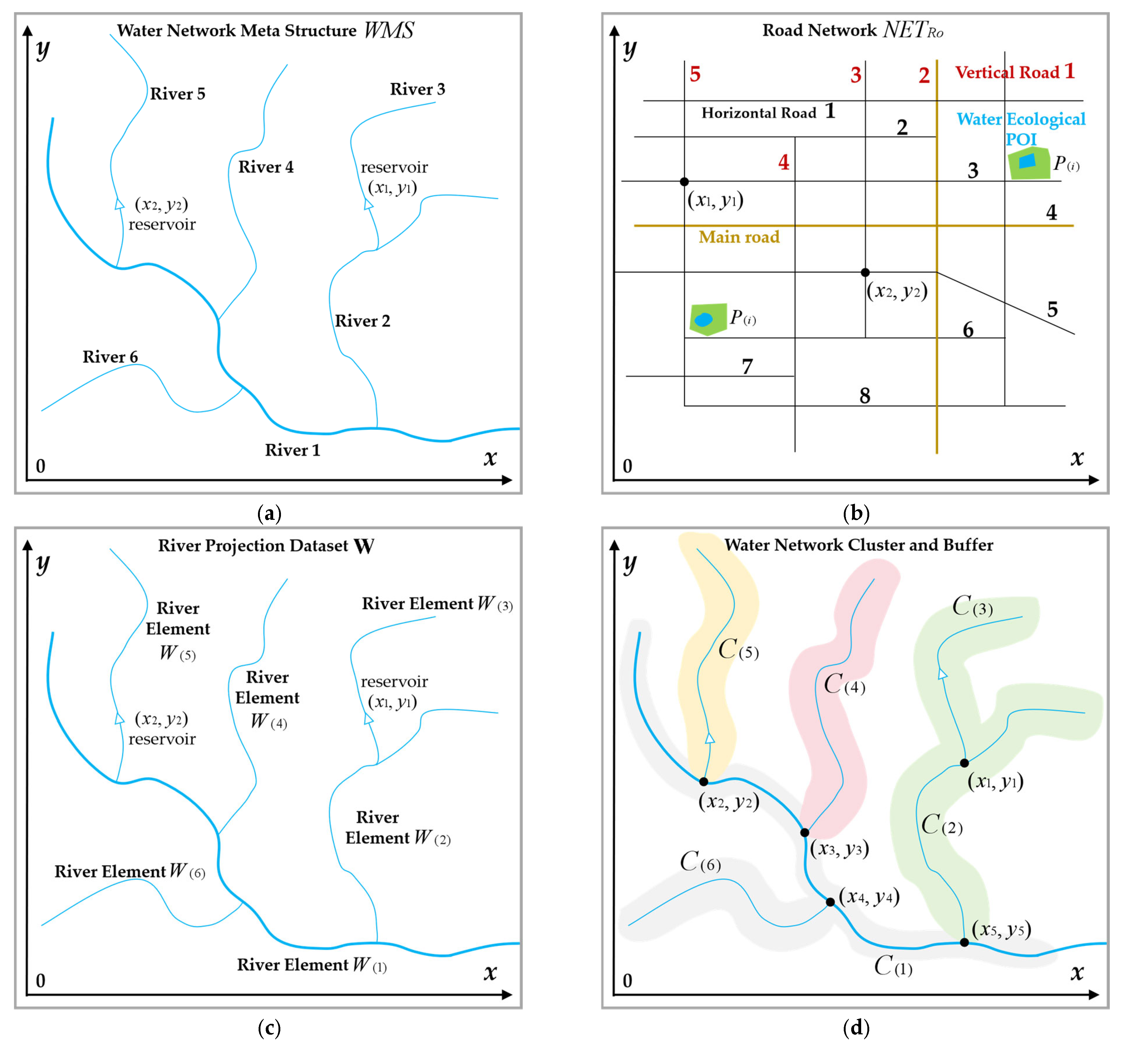
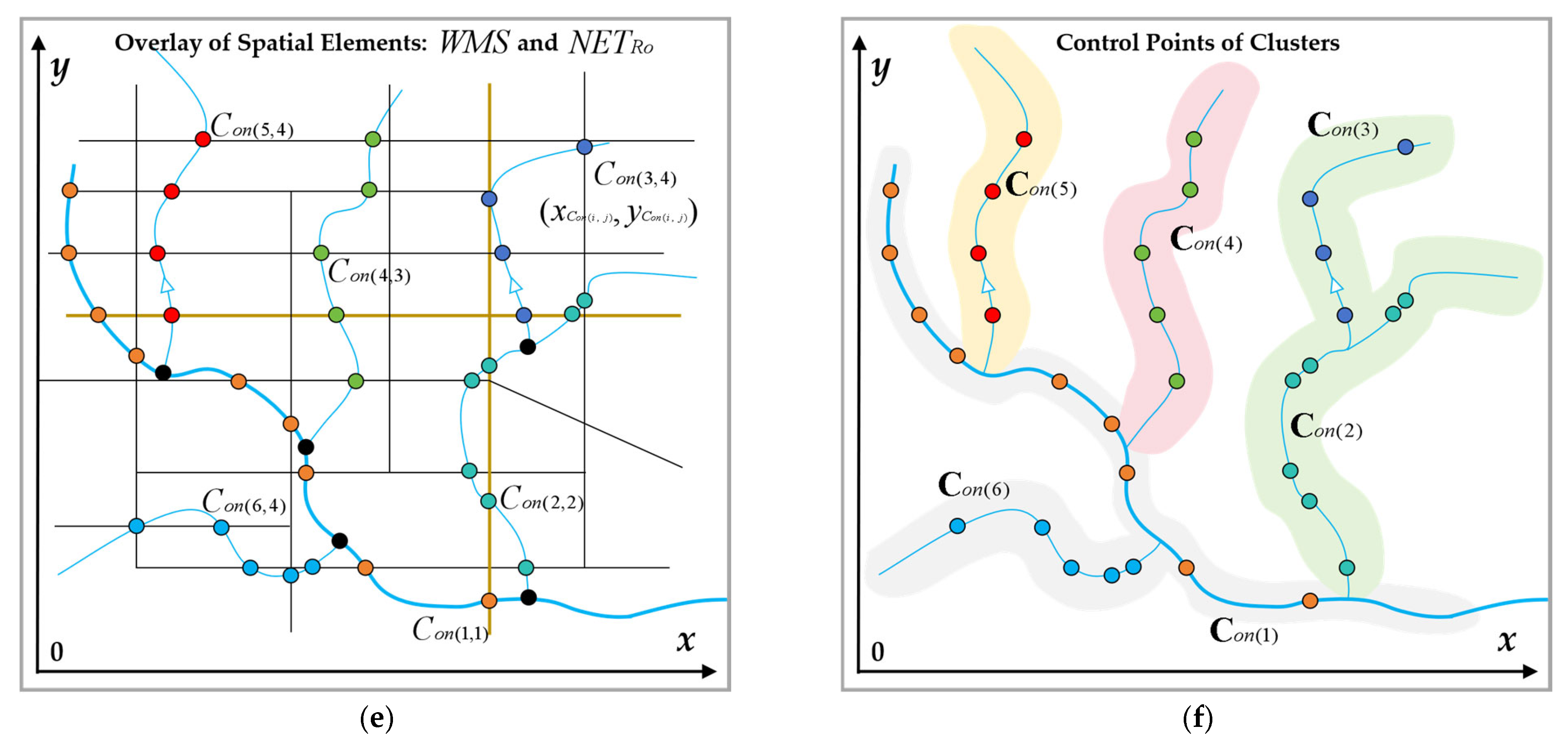
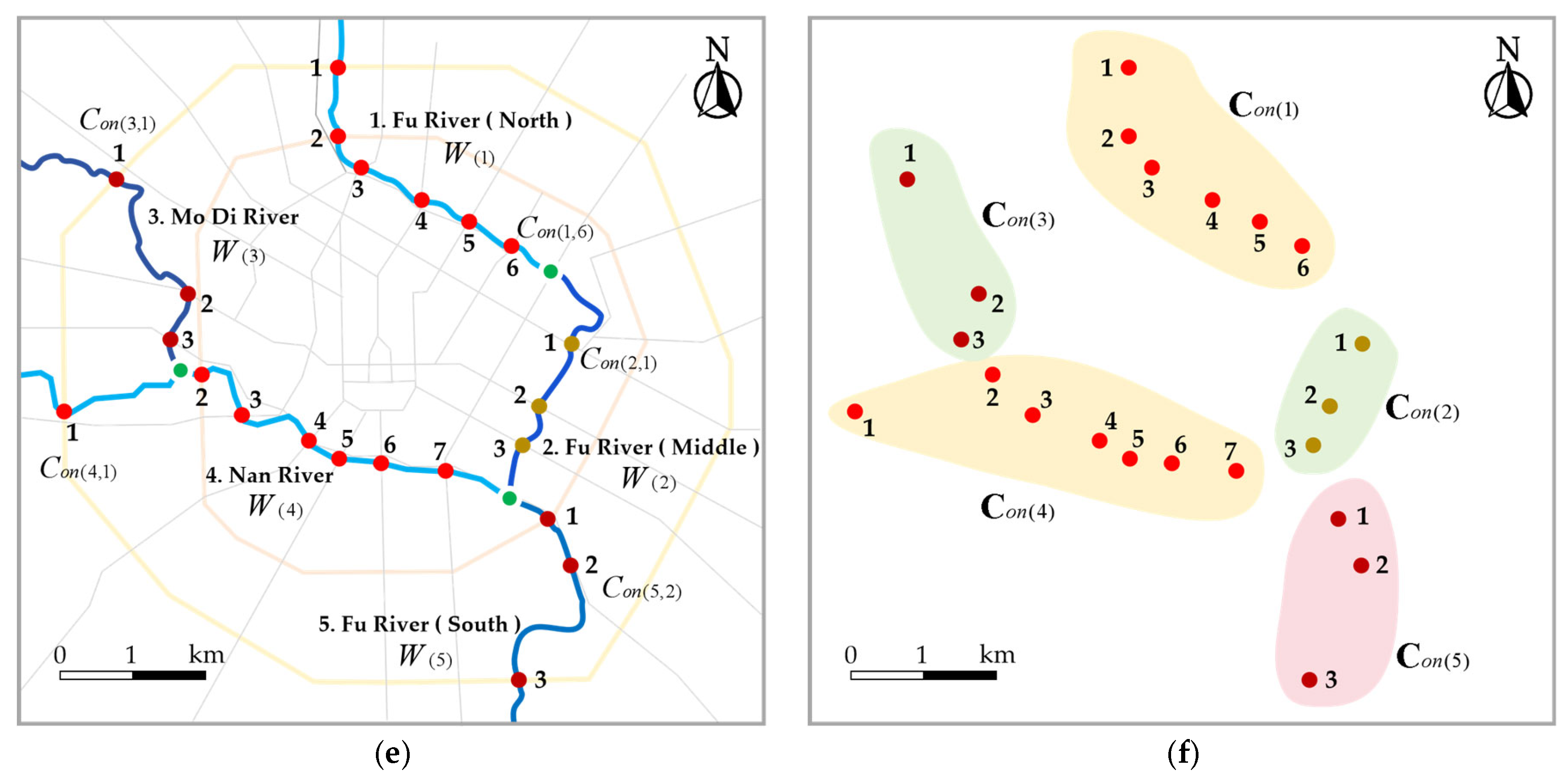
According to the definition, Figure 2 shows the generating process of the ${NET}_{Ro}$, $WMS$, dataset $W$ and elements $W_{(i)}$, cluster $C_{(i)}$ buffer zones, and control point sets $C_{on(i)}$ by the urban water network channels and main roads in the coordinate system $xoy$. Among them, Figure 2a shows the constructed main water network meta-structure ($WMS$), Figure 2b shows the constructed main road network (${NET}_{Ro}$), Figure 2c shows the constructed river projection dataset $W$, Figure 2d shows the constructed water network cluster $C_{(i)}$ and the buffer zone, Figure 2e shows the overlay model of $WMS$ and ${NET}_{Ro}$, and Figure 2f shows the constructed cluster control point set $C_{on(i)}$.

The objective function for constructing the cluster $C_{(i)}$ is defined as $f_{[P_{(i)},C_{on(i,j)}]}$, and its calculating criterion is the spatial accessibility of $P_{(i)}$ to $C_{on(i,j)}$. The spatial accessibility model $S_{A[P_{(i)},C_{on(i,j)}]}$ is constructed as in the Formula (4), and ${\delta }_{(1)}$ is the dimensionality reduction parameter. The definition of value ${\delta }_{(1)}$ is as follows:

(1) If the spatial distance $d$ between $P_{(i)}$ and $C_{on(i,j)}$ meets $d\in (0,1)$, ${\delta }_{(1)}=1$;

(2) If the spatial distance $d$ between $P_{(i)}$ and $C_{on(i,j)}$ meets $d\in [1,10)$, ${\delta }_{(1)}=0.1$;

(3) If the spatial distance $d$ between $P_{(i)}$ and $C_{on(i,j)}$ meets $d\in [10,100)$, ${\delta }_{(1)}=0.01$; and so forth.

$$S_{A[P_{(i)},C_{on(i,j)}]}={\delta }_{(1)}\times {\left[{\left(x_{P(i)}-x_{Con(i,j)}\right)}^2+{\left(y_{P(i)}-y_{C_{on(i,j)}}\right)}^2\right]}^{{\displaystyle \frac{1}{2}}}$$

(4)

Based on Formula (4), construct the function $f_{[P_{(i)},C_{on(i,j)}]}$ as the Formulas (5) and (6), and ${\delta }_{(2)}$ is the dimensionality reduction parameter. The definition of value ${\delta }_{(2)}$ is as follows:

(1) If the reciprocal of $S_{A[P_{(i)},C_{on(i,j)}]}$ meets $d\in (0,1)$, ${\delta }_{(2)}=1$;

(2) If the reciprocal of $S_{A[P_{(i)},C_{on(i,j)}]}$ meets $d\in [1,10)$, ${\delta }_{(2)}=0.1$;

(3) If the reciprocal of $S_{A[P_{(i)},C_{on(i,j)}]}$ meets $d\in [10,100)$, ${\delta }_{(2)}=0.01$; and so forth.

$$f_{[P_{(i)},C_{on(i,j)}]}={\delta }_{(2)}\times {\displaystyle \frac{1}{S_{A[P_{(i)},C_{on(i,j)}]}}}$$

(5)

$$f_{[P_{(i)},C_{on(i,j)}]}={\displaystyle \frac{{\delta }_{(2)}}{{\delta }_{(1)}}}\times {\left[{\left(x_{P(i)}-x_{Con(i,j)}\right)}^2+{\left(y_{P(i)}-x_{Con(i,j)}\right)}^2\right]}^{-{\displaystyle \frac{1}{2}}}$$

(6)

Based on the set $C_{on(i)}$ and the dimension $t_{(i)}$ of $W_{(i)}$, a complete binary tree $T_{W(i)}$ with $t_{(i)}$ number of nodes is constructed, and it is defined as the complete binary tree for the water ecological POI clustering. The tree $T_{W(i)}$ node $N_{ode(i,j)}$ stores the function value $f_{[P_{(i)},C_{on(i,j)}]}$, and its structure satisfies the following conditions:

(1) The height of the tree is $d$, and the parent node level is 0. Therefore, all the child nodes are at No. $i$ level, $0<i\le d$, $i,d\in N$, and for any node $N_{ode(i,j)}$, it can contain at most 2 child nodes and at least no child nodes;

(2) When $d\ge 1$, the No. $d-1$ layer contains $2^{d-1}$ number of nodes;

(3) If there are child nodes in the No. $i$ layer, all the child nodes are concentrated on the leftmost side;

(4) For any No. $d-1$ layer node and No. $d$ layer node, satisfy $N_{ode(d-1,\forall j)}\ge N_{ode(d,\forall j)}$;

(5) For any No. $d$ layer, satisfy $N_{ode(d,j)}\ge N_{ode(d,j+1)}$;

(6) If a node $N_{ode(i,j)}$ contains only one child node, it must satisfy the condition of node $\forall N_{ode(i,x)}$ not containing any child node, $x>j$.

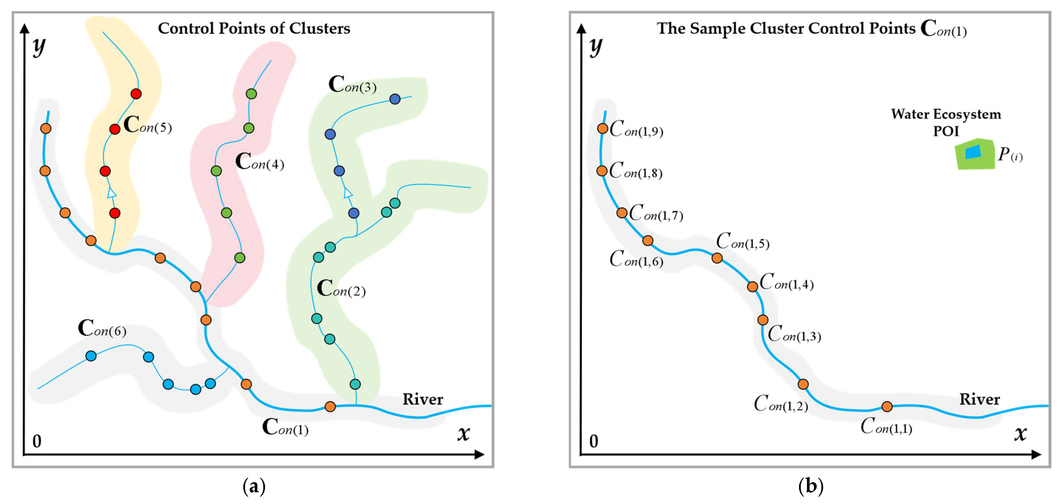
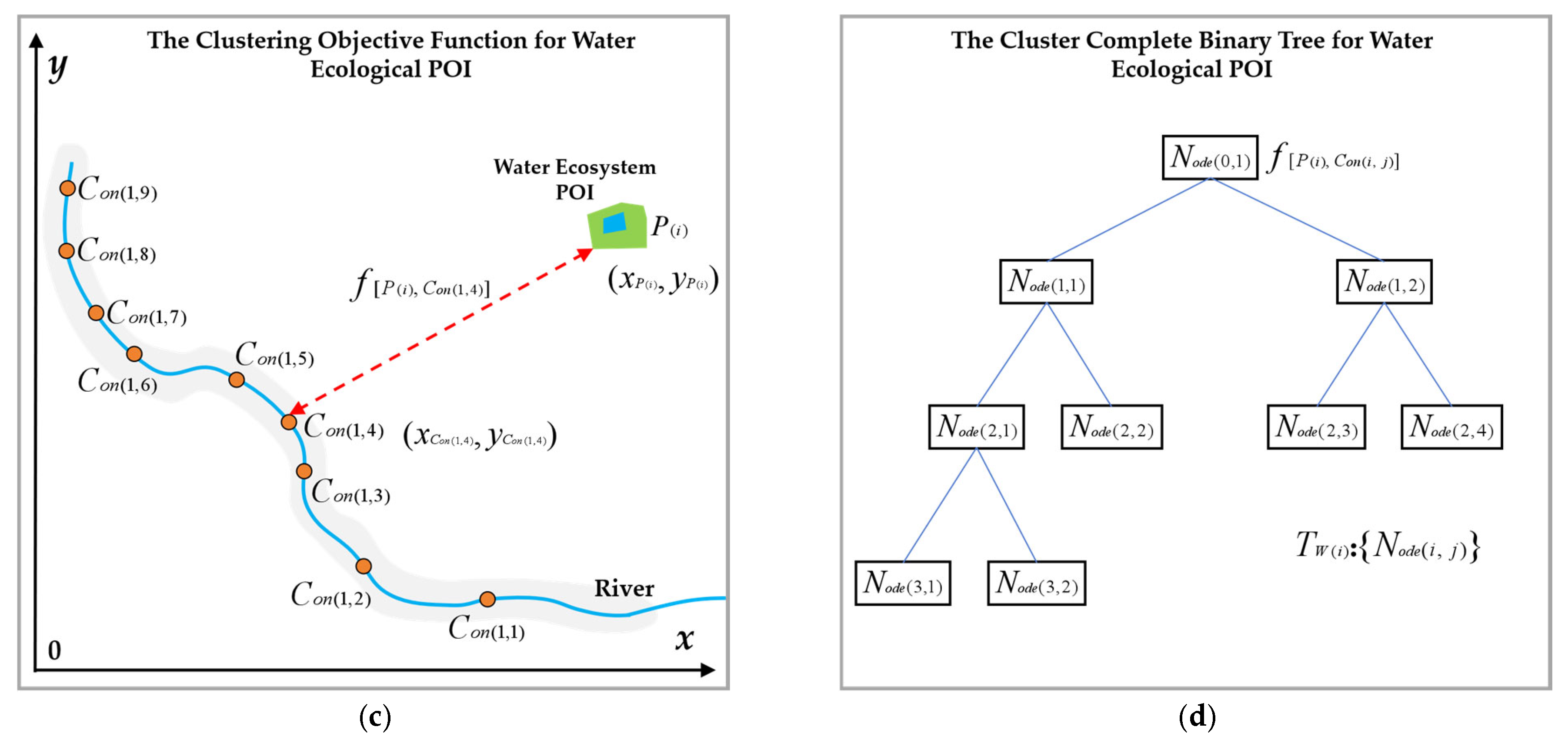
Figure 3 shows the process of constructing the complete binary tree $T_{W(i)}$ based on the river channel elements $W_{(i)}$ and the control point sets $C_{on(i)}$. Figure 3a shows the cluster control point sets $C_{on(i)}$, Figure 3b shows the selected sample cluster control point set $C_{on(1)}$, Figure 3c shows the water ecological POI clustering objective function model $f_{[P_{(i)},C_{on(i,j)}]}$, and Figure 3d shows the generated water ecological POI clustering complete binary tree $T_{W(i)}$ based on $C_{on(1)}$. The complete binary tree $T_{W(i)}$ is the key model for constructing the clustering algorithm [25].

The water ecological POI spatial clustering model based on the improved water network space AGNES algorithm is constructed as follows. Figure 4 shows the process of constructing the clustering algorithm model [26]:

Step 1: Collect and model the river water network data.

(1) Construct the coordinate system $xoy$.

(2) Determine the $N$ number of water ecological POI elements $P_{(i)}$ to be clustered and their coordinates $x_{P_{(i)}}$ and $y_{P_{(i)}}$.

(3) Based on the urban geospatial data, construct ${NET}_{Ro}$ and $WMS$.

(4) Extract $m$ number of river channel elements $W_{(i)}$ from the $WMS$ and construct the dataset $W$.

Step 2: Model the control point set and construct the matrix ${\mathbf{M}}_{\mathrm{C}on}$.

(1) Project the ${NET}_{Ro}$ and $WMS$ to form the coordinate system $xoy$.

(2) Take the element $W_{(1)}$ in $W$, determine the control points $C_{on(1,j)}$ formed by the intersection of ${NET}_{Ro}$ and $W_{(1)}$ and construct control point set $C_{on(1)}$, store them in the corresponding first row of the matrix ${\mathbf{M}}_{\mathrm{C}on}$, and determine the row rank $t_{(1)}$.

(3) Take the element $W_{(2)}$ in $W$, determine the control points $C_{on(2,j)}$ formed by the intersection of ${NET}_{Ro}$ and $W_{(2)}$ and construct the control point set $C_{on(2)}$, store them in the corresponding second row of the matrix ${\mathbf{M}}_{\mathrm{C}on}$, and determine the row rank $t_{(2)}$.

(4) Repeat the above steps. Take $\forall W_{(i)}$, traverse $0<i\le m$, determine the control points $C_{on(i,j)}$ formed by the intersection of ${NET}_{Ro}$ and $W_{(i)}$ and construct the control point set $C_{on(i)}$, store them in the corresponding No. $i$ row of the matrix ${\mathbf{M}}_{\mathrm{C}on}$, and determine the row rank $t_{(i)}$, till the matrix ${\mathbf{M}}_{\mathrm{C}on}$ arrives at full rank.

(5) Determine the coordinates $x_{Con(i,j)}$ and $y_{Con(i,j)}$ of each control point $C_{on(i,j)}$.

Step 3: Build the spatial relationship model between the water ecological POI element $\forall P_{(i)}$ and the element $\forall W_{(i)}$, and extract $P_{(1)}$ from the entire POI element set.

(1) Take the first row point set $C_{on(1)}$ of the matrix ${\mathbf{M}}_{\mathrm{C}on}$, with row rank $t_{(1)}$ and row elements $C_{on(1,j)}$, corresponding to the river channel element $W_{(1)}$.

(2) Construct a complete binary tree with $t_{(1)}$ number of nodes, denoted as $N_{ode(i,j)}$.

(3) Calculate $f_{[P_{(1)},C_{on(1,j)}]}$, subscript $j$ traverses $0<j\le t_{(1)}$. Compare $f_{[P_{(1)},C_{on(1,1)}]}$ and $f_{[P_{(1)},C_{on(1,2)}]}$:

① If $f_{[P_{(1)},C_{on(1,1)}]}\ge f_{[P(1),C_{on(1,2)}]}$, store $f_{[P_{(1)},C_{on(1,1)}]}$ to the parent node $N_{ode(0,1)}$ and store $f_{[P_{(1)},C_{on(1,2)}]}$ to the child node $N_{ode(1,1)}$.

② If $f_{[P_{(1)},C_{on(1,1)}]}<f_{[P_{(1)},C_{on(1,2)}]}$, store $f_{[P_{(1)},C_{on(1,2)}]}$ to the parent node $N_{ode(0,1)}$ and store $f_{[P_{(1)},C_{on(1,1)}]}$ to the child node $N_{ode(1,1)}$.

(4) Take $f_{[P_{(1)},C_{on(1,3)}]}$, Compare $f_{[P_{(1)},C_{on(1,1)}]}$ and $f_{[P_{(1)},C_{on(1,2)}]}$:

① If $f_{[P_{(1)},C_{on(1,1)}]}\ge f_{[P_{(1)},C_{on(1,2)}]}$:

(i) If $f_{[P_{(1)},C_{on(1,3)}]}\ge f_{[P_{(1)},C_{on(1,1)}]}\ge f_{[P_{(1)},C_{on(1,2)}]}$, store $f_{[P_{(1)},C_{on(1,3)}]}$, $f_{[P_{(1)},C_{on(1,1)}]}$ and $f_{[P_{(1)},C_{on(1,2)}]}$ to the parent node $N_{ode(0,1)}$, child node $N_{ode(1,1)}$ and $N_{ode(1,2)}$.

(ii) If $f_{[P_{(1)},C_{on(1,1)}]}>f_{[P_{(1)},C_{on(1,3)}]}\ge f_{[P_{(1)},C_{on(1,2)}]}$, store $f_{[P_{(1)},C_{on(1,1)}]}$, $f_{[P_{(1)},C_{on(1,3)}]}$ and $f_{[P_{(1)},C_{on(1,2)}]}$ to the parent node $N_{ode(0,1)}$, child node $N_{ode(1,1)}$ and $N_{ode(1,2)}$.

(iii) If $f_{[P_{(1)},C_{on(1,1)}]}\ge f_{[P_{(1)},C_{on(1,2)}]}\ge f_{[P_{(1)},C_{on(1,3)}]}$, store $f_{[P_{(1)},C_{on(1,1)}]}$, $f_{[P_{(1)},C_{on(1,2)}]}$ and $f_{[P_{(1)},C_{on(1,3)}]}$ to the parent node $N_{ode(0,1)}$, child node $N_{ode(1,1)}$ and $N_{ode(1,2)}$.

② If $f_{[P_{(1)},C_{on(1,1)}]}<f_{[P_{(1)},C_{on(1,2)}]}$:

(i) If $f_{[P_{(1)},C_{on(1,1)}]}<f_{[P_{(1)},C_{on(1,2)}]}\le f_{[P_{(1)},C_{on(1,3)}]}$, store $f_{[P_{(1)},C_{on(1,3)}]}$, $f_{[P_{(1)},C_{on(1,2)}]}$ and $f_{[P_{(1)},C_{on(1,1)}]}$ to the parent node $N_{ode(0,1)}$, child node $N_{ode(1,1)}$ and $N_{ode(1,2)}$.

(ii) If $f_{[P_{(1)},C_{on(1,1)}]}<f_{[P_{(1)},C_{on(1,3)}]}<f_{[P_{(1)},C_{on(1,2)}]}$, store $f_{[P_{(1)},C_{on(1,2)}]}$, $f_{[P_{(1)},C_{on(1,3)}]}$ and $f_{[P_{(1)},C_{on(1,1)}]}$ to the parent node $N_{ode(0,1)}$, child node $N_{ode(1,1)}$ and $N_{ode(1,2)}$.

(iii) If $f_{[P_{(1)},C_{on(1,3)}]}\le f_{[P_{(1)},C_{on(1,1)}]}<f_{[P_{(1)},C_{on(1,2)}]}$, store $f_{[P_{(1)},C_{on(1,2)}]}$, $f_{[P_{(1)},C_{on(1,1)}]}$ and $f_{[P_{(1)},C_{on(1,3)}]}$ to the parent node $N_{ode(0,1)}$, child node $N_{ode(1,1)}$ and $N_{ode(1,2)}$.

(5) Repeat the above steps, take $f_{[P_{(1)},C_{on(1,1)}]}$, $f_{[P_{(1)},C_{on(1,2)}]}$,…, $f_{[P_{(1)},C_{on(1,j)}]}$ and make a comparison. According to the binary tree storage rules, store the elements $f_{[P_{(1)},C_{on(1,j)}]}$ to each node $N_{ode(i,j)}$ of the binary tree $T_{W(i)}$.

(6) When the traversal $f_{[P_{(1)},C_{on(1,j)}]}$ is complete, $j=t_{(1)}$, the binary tree $T_{W(1)}$ is stored and forms a large tree. The function value $f_{[P_{(1)},C_{on(1,j)}]}$ stored in the current parent node $N_{ode(0,1)}$ is the optimal spatial relationship value between the POI element $P_{(1)}$ and river element $W_{(1)}$, denoted as ${f_{[P_{(1)},C_{on(1,j)}]}}^{\max }$.

(7) Return to Step (1), take the second row point set $C_{on(2)}$ of the matrix ${\mathbf{M}}_{\mathrm{C}on}$, with row rank $t_{(2)}$ and row element $C_{on(2,j)}$, corresponding to the river channel element $W_{(2)}$. Calculate the function values $f_{[P_{(1)},C_{on(2,j)}]}$ between the POI element $P_{(1)}$ and elements $C_{on(2,j)}$. Traverse $0<j\le t_{(2)}$ and store the elements $f_{[P_{(1)},C_{on(2,j)}]}$ to each node $N_{ode(i,j)}$ of the binary tree $T_{W(i)}$ according to the storage rules of the binary tree. The function value $f_{[P_{(1)},C_{on(2,j)}]}$ stored in the current parent node $N_{ode(0,1)}$ is the optimal spatial relationship value between the POI element $P_{(1)}$ and river channel element $W_{(2)}$, denoted as ${f_{[P_{(1)},C_{on(2,j)}]}}^{\max }$.

(8) Repeat steps (1) to (6) until all rows $i=m$ of the matrix ${\mathbf{M}}_{\mathrm{C}on}$ form a binary tree $T_{W(i)}$, resulting in $m$ number of binary trees with stored value ${f_{[P_{(1)},C_{on(i,j)}]}}^{\max }$ for each tree’s parent node $N_{ode(0,1)}$.

(9) Build a complete binary tree containing $m$ number of nodes, traverse all the stored values ${f_{[P_{(1)},C_{on(i,j)}]}}^{\max }$ of the parent nodes of the river element binary trees, and store them in the complete binary tree according to the storage rules of the complete binary tree. Take the element value ${f_{[P_{(1)},C_{on(i,j)}]}}^{\max }$ corresponding to the parent node as the maximum value ${\max f_{[P_{(1)},C_{on(i,j)}]}}^{\max }$ of all the river element binary trees. Search for the corresponding row $i$ of matrix ${\mathbf{M}}_{\mathrm{C}on}$, and the related No. $i$ channel element is the cluster $C_{(i)}$ corresponding to the POI element $P_{(1)}$.

(10) Store the POI element $P_{(1)}$ in the first element position of the cluster $C_{(i)}$ row corresponding to the No. $i$ channel element $W_{(i)}$ in the clustering matrix $C$. The clustering process of the POI element $P_{(1)}$ ends.

Step 4: Return to Step 3 and extract $P_{(2)}$ from the set of all the POI elements.

(1) According to the Step 3 algorithm, output a complete binary tree $T_{W(i)}$ of all the river channel elements $W_{(i)}$ in the dataset $W$ corresponding to $P_{(2)}$, and output $m$ number of parent nodes ${f_{[P_{(2)},C_{on(i,j)}]}}^{\max }$.

(2) Build a binary tree of the river channel elements containing $m$ number of nodes, and take the corresponding element ${f_{[P_{(2)},C_{on(i,j)}]}}^{\max }$ of its parent node.

(3) Search for the corresponding row $i$ of matrix ${\mathbf{M}}_{\mathrm{C}on}$, and the corresponding No. $i$ channel element is the cluster $C_{(i)}$ corresponding to the POI element $P_{(2)}$.

(4) Judge the first element position of the cluster row $C_{(i)}$ corresponding to the No. $i$ river channel element $W_{(i)}$ in the clustering matrix $C$. If it is an empty element, store the POI element $P_{(2)}$. If it is a non-empty element, store it in the second element. The clustering process of the POI element $P_{(2)}$ ends.

Step 5: Continue searching for other POI elements $P_{(i)}$ and then calculate ${{\max f}_{[P_{(i)},C_{on(i,j)}]}}^{\max }$ according to the algorithm from Step 3 to Step 4. Search for the corresponding row $i$ of matrix ${\mathbf{M}}_{\mathrm{C}on}$. The corresponding No. $i$ channel element is the cluster $C_{(i)}$ corresponding to the POI element $P_{(i)}$, and the POI element $P_{(i)}$ is stored in $C_{(i)}$. Traverse $2<i\le N$ until the No. $P_{(N)}$ element is stored in the matrix $C$. Output the clustering matrix $C$.

3.2. Logistics Distribution Center Location Model Based on Water Ecological POI Clustering

The modeling basis of the POI logistics route-planning algorithm is to select the material distribution center as the starting and ending points of the route, and the water ecological POIs that require material distribution as route nodes. The route completes the delivery in a certain order. Under the constraints of the urban geographic space, the key condition for controlling the logistics costs and pollutant emissions is to determine the spatial relationship between the distribution center of assembly materials and the water ecological POIs. That is, when the water ecological POIs to be delivered are determined, the optimal location of the distribution center is achieved by constructing a spatial relationship model between the distribution center and POIs to ensure that the materials depart from the optimal location of the distribution center and minimize the logistics costs and pollutant emissions [27,28]. Based on the modeling idea, we established a logistics distribution center location model based on the water ecological POI clustering, the distribution center dataset, and the POI dataset to be delivered. The material assembly points with material reserve capacity in the city are defined as the distribution centers $D_{(i)}$. Its coordinates are denoted as $x_{D(i)}$ and $y_{D(i)}$. The distribution center is the starting and ending point of the POI logistics route. The number of candidate distribution centers is $g$.

Definition 5. 

The closeness between  $D_{(i)}$ and cluster  $C_{(i)}$ is determined by the closeness algorithm between the control points of  $C_{(i)}$  and  $D_{(i)}$. Define the closeness model  $f_{[D_{(i)},C_{on(i,j)}]}$ as Formula (7). The value rules for parameters  ${\delta }_{(1)}$ and  ${\delta }_{(2)}$ are the same as Formulas (4)–(6):

$$f_{[D_{(i)},C_{on(i,j)}]}={\displaystyle \frac{{\delta }_{(2)}}{{\delta }_{(1)}}}\times {\left[{\left(x_{D(i)}-x_{Con(i,j)}\right)}^2+{\left(y_{D(i)}-y_{Con(i,j)}\right)}^2\right]}^{-{\displaystyle \frac{1}{2}}}$$

(7)

Definition 6. 

The spatial relationship between  $D_{(i)}$ and POIs to be delivered is defined as the closeness model  $f_{[D_{(i)},P_{(i)}]}$, as shown in Formula (8). When the number of POIs to be delivered is  $n$, the average closeness model between  $D_{(i)}$  and  $n$ number of POIs  $P_{(x)}$ is defined as  ${\overline{f}}_{[D_{(i)},P_{(i)}]}$, as shown in Formula (9). The value rules for parameters  ${\delta }_{(1)}$  and  ${\delta }_{(2)}$ are the same as Formulas (4)–(6):

$$f_{[D_{(i)},P_{(i)}]}={\displaystyle \frac{{\delta }_{(2)}}{{\delta }_{(1)}}}\times {\left[{\left(x_{D(i)}-x_{P(i)}\right)}^2+{\left(y_{D(i)}-y_{P(i)}\right)}^2\right]}^{-{\displaystyle \frac{1}{2}}}$$

(8)

$${\overline{f}}_{[D_{(i)},P_{(i)}]}={\displaystyle \frac{1}{n}}\times {\displaystyle \sum _{x=1}^n{f}_{[D_{(i)},P_{(x)}]}}$$

(9)

Definition 7. 

Construct a  $m\times g$ dimension matrix to store the closeness relationship between  $D_{(i)}$  and  $C_{(i)}$. The No.  $i$ row represents the No.  $i$ cluster  $C_{(i)}$, and the column represents the No.  $j$ center  $D_{(i)}$ with the highest closeness value to  $C_{(i)}$. Formula (9) is the matrix  $C_{D(i)}$,  $D_{(i,j)}$ represents  $D_{(i)}$, and  $g_{(i)}$  represents that there are  $g_{(i)}$ number of  $D_{(i)}$  with high closeness values in  $C_{(i)}$:

$$C_{D(i)}=\left[\begin{array}{cccccc}{D}_{(1,1)}& D_{(1,2)}& \dots & D_{(1,j)}& \dots & D_{(1,g_{(1)})}\\ D_{(2,1)}& D_{(2,2)}& \dots & D_{(2,j)}& \dots & D_{(2,g_{(2)})}\\ \dots & \dots & \dots & \dots & \dots & \dots \\ D_{(i,1)}& D_{(i,2)}& \dots & D_{(i,j)}& \dots & D_{(i,g_{(i)})}\\ \dots & \dots & \dots & \dots & \dots & \dots \\ D_{(m,1)}& D_{(m,2)}& \dots & D_{(m,j)}& \dots & D_{(m,g_{(m)})}\end{array}\right]$$

(10)

The relationship between $D_{(i)}$ and cluster $C_{(i)}$ is determined by the closeness model $f_{[D_{(i)},C_{on(i,j)}]}$ and could be transformed into a closeness relationship with the control points $C_{on(i,j)}$ of the river element $W_{(i)}$ to $D_{(i)}$. We construct a complete binary tree containing $t_{(i)}$ number of nodes for storing the closeness values $f_{[D_{(i)},C_{on(i,j)}]}$. This binary tree is defined as the distribution center closeness complete binary tree, denoted as ${T_{D(i)}}^{[j]}$. Among them, $t_{(i)}$ represents the number of control points for rivers $W_{(i)}$, that is, the number of control points for the cluster $C_{(i)}$. The subscript $i$ corresponds to the No. $i$ distribution center $D_{(i)}$, and the superscript $j$ indicates the closeness relationship with the No. $j$ cluster $C_{(j)}$. Corresponding to $m$ number of clusters $C_{(i)}$, the $m$ number of complete binary trees ${T_{D(i)}}^{[j]}$ output $m$ number of parent nodes, $0<j\le m$, $j,m\in N$, and the cluster corresponding to the optimal parent node is the cluster with the highest degree of closeness to the distribution center. Then, calculate the $g$ number of ${\overline{f}}_{[D_{(i)},P_{(i)}]}$ between $g$ number of the candidate distribution centers $D_{(i)}$ and $n$ number of the POIs $P_{(i)}$ to be delivered. We construct a complete binary tree containing $g$ number of nodes to store the values ${\overline{f}}_{[D_{(i)},P_{(i)}]}$. This binary tree is defined as the distribution center optimal location, a complete binary tree, denoted as ${T_{D(i)}}^{opt}$.

We constructed the logistics distribution center location model based on water ecological POI clustering to determine the optimal starting and ending points of water ecological POI logistics routes. Figure 5 shows the process of constructing the distribution center location algorithm model:

Step 1: Collect the basic modeling data.

(1) Determine the $g$ number of candidate distribution centers $D_{(i)}$ and their coordinates $x_{D(i)}$ and $y_{D(i)}$ in the urban coordinate system $xoy$.

(2) Determine the $n$ number of POI elements $P_{(i)}$ to be delivered and the coordinates $x_{P_{(i)}}$ and $y_{P_{(i)}}$.

(3) Determine the control points $C_{on(i,j)}$ and coordinates $x_{C_{on(i,j)}}$ and $y_{C_{on(i,j)}}$ of all clusters $C_{(i)}$ corresponding to the river channels $W_{(i)}$.

(4) Establish the closeness matrix $C_{D(i)}$.

Step 2: Build the closeness relationship between $g$ number of candidate distribution centers $D_{(i)}$ and $m$ number of clusters $C_{(i)}$. Select the distribution center $D_{(1)}$ and cluster $C_{(1)}$, and construct the distribution center closeness complete binary tree ${T_{D(1)}}^{[1]}$.

(1) Take the first row of the control points $C_{on(1)}$ in the cluster matrix ${\mathbf{M}}_{\mathrm{C}on}$, with row rank $t_{(1)}$ and row element $C_{on(1,j)}$, corresponding to the river channel element $W_{(1)}$ and cluster $C_{(1)}$.

(2) Construct a complete binary tree with a node number count of $t_{(1)}$, denoted as ${T_{D(1)}}^{[1]}$.

(3) Traverse the subscripts from 1 to $j$ and calculate $f_{[D_{(1)},C_{on(1,j)}]}$.

(4) Compare the current $f_{[D_{(1)},C_{on(1,1)}]}$, $f_{[D_{(1)},C_{on(1,2)}]}$,…, $f_{[D_{(1)},C_{on(1,\mathrm{j})}]}$. Nodes 1 to Note $j$ are stored according to the maximum complete binary tree rule.

(5) Repeat steps (3) to (4) until $j=t_{(1)}$, the traversal is complete, and the output is ${T_{D(1)}}^{[1]}$.

(6) Take the parent node $N_{ode(0,1)}$ and the corresponding function value ${\max f}_{[D_{(1)},C_{on(1,j)}]}$ of the binary tree ${T_{D(1)}}^{[1]}$.

Step 3: Return to Step 2, select the distribution center $D_{(1)}$ and cluster $C_{(i)}$, and construct the distribution center closeness complete binary tree ${T_{D(1)}}^{[1]}$.

(1) Take the No. $i$ row of the control points $C_{on(i)}$ in the cluster matrix $M_{\mathrm{C}on}$, with row rank $t_{(i)}$ and row element $C_{on(i,j)}$, corresponding to the river channel element $W_{(i)}$ and cluster $C_{(i)}$.

(2) Construct a complete binary tree with a node number count of $t_{(i)}$, denoted as ${T_{D(1)}}^{[i]}$.

(3) Traverse the subscripts from 1 to $j$ and calculate $f_{[D_{(1)},C_{on(i,j)}]}$.

(4) Compare the current $f_{[D_{(1)},C_{on(i,1)}]}$, $f_{[D_{(1)},C_{on(i,2)}]}$,…, $f_{[D_{(1)},C_{on(i,j)}]}$. Nodes 1 to Note $j$ are stored according to the maximum complete binary tree rule.

(5) Repeat steps (3) to (4) until $j=t_{(i)}$, the traversal is complete, and the output is ${T_{D(1)}}^{[1]}$.

(6) Take the parent node $N_{ode(0,1)}$ and the corresponding function value ${\max f}_{[D_{(1)},C_{on(i,j)}]}$ of the binary tree ${T_{D(1)}}^{[1]}$.

Step 4: Repeat the algorithm from Step 2 to Step 3 and traverse the cluster $C_{(i)}$ subscripts $0<i\le m$.

(1) Output the closeness values ${\max f}_{[D_{(1)},C_{on(i,j)}]}$ between the distribution center $D_{(1)}$ and $m$ number of clusters.

(2) Select $\max \{\max f_{[D_{(1)},C_{on(i,j)}]}\}$ and determine its corresponding cluster $C_{(i)}$, which has the highest degree of closeness with the distribution center $D_{(1)}$.

(3) Store $D_{(1)}$ in the No. $i$ row corresponding to the cluster in the closeness matrix $C_{D_{(i)}}$.

Step 5: Return to Step 2 and calculate according to the algorithm from Step 2 to Step 4.

(1) Traverse $1<x\le g$ and calculate the closeness relationship between distribution center $D_{(x)}$ and cluster $C_{(i)}$.

(2) Select $\max \{\max f_{[D_{(x)},C_{on(i,j)}]}\}$ and determine its corresponding cluster $C_{(i)}$, which has the highest degree of closeness with the distribution center $D_{(x)}$.

(3) Store $D_{(x)}$ in the No. $i$ row corresponding to the cluster in the closeness matrix $C_{D_{(i)}}$.

(4) For the distribution center $D_{(x)}$, after traversal $x=g$, output a full ranked matrix $C_{D_{(i)}}$. The No. $i$ row of the matrix corresponds to the distribution centers $D_{(i)}$ with the highest closeness values for the cluster.

Step 6: Search for $n$ number of water ecological POI elements $P_{(i)}$ to be delivered. Initialize the counter ${count}_{[i]}=0$, in which ${count}_{[i]}$ represents the number of occurrences for the cluster $C_{(i)}$.

(1) Search for element $P_{(1)}$, determine $P_{(1)}\in C_{(i)}$, and iterate ${count}_{[i]}={count}_{[i]}+1$ for the counter of cluster $C_{(i)}$.

(2) Search for element $P_{(2)}$, determine $P_{(2)}\in C_{(i)}$, and iterate ${count}_{[i]}={count}_{[i]}+1$ for the counter of cluster $C_{(i)}$.

(3) Repeat the above search. Search for the element $P_{(x)}$, determine $P_{(x)}\in C_{(i)}$, and iterate ${count}_{[i]}={count}_{[i]}+1$ for the counter of cluster $C_{(i)}$.

(4) Traverse $1<x\le n$ until all the water ecological POI elements have been searched.

(5) Count ${count}_{[i]}$ for each cluster and select the corresponding cluster of $\max {count}_{[i]}$ as the optimal location cluster, denoted as ${C_{(i)}}^{opt}$.

Step 7: Locate the row in the matrix $C_{D_{(i)}}$ for ${C_{(i)}}^{opt}$, in which all the distribution centers $D_{(i)}$ are the candidate elements for the optimal distribution center, with a quantity of $q$. Construct a complete binary tree ${T_{D(i)}}^{opt}$ for the optimal location of distribution centers with $q$ number of candidate distribution centers $D_{(i)}$ as nodes.

(1) Note $q$ number of candidate distribution centers $D_{(i)}$ as ${D_{(i)}}^{\mathsf{\Delta }}$, $0<i\le q$, $i,q\in N$.

(2) Determine the coordinates ${x_{D(i)}}^{\mathsf{\Delta }}$ and ${y_{D(i)}}^{\mathsf{\Delta }}$ of each distribution center ${D_{(i)}}^{\mathsf{\Delta }}$, and identify the $n$ number of water ecological POI elements $P_{(i)}$ to be delivered and their coordinates $x_{P_{(i)}}$ and $y_{P_{(i)}}$.

(3) Construct a complete binary tree with a node number count of $q$, denoted as ${T_{D(i)}}^{opt}$.

(4) For ${D_{(1)}}^{\mathsf{\Delta }}$, traverse subscripts from 1 to $n$, and calculate ${\overline{f}}_{[{D_{(1)}}^{\mathsf{\Delta }},P(j)]}$.

(5) For ${D_{(2)}}^{\mathsf{\Delta }}$, traverse subscripts from 1 to $n$, and calculate ${\overline{f}}_{[{D_{(2)}}^{\mathsf{\Delta }},P(j)]}$.

(6) Repeat steps (4) to (5), traverse $0<i\le q$, for ${D_{(i)}}^{\mathsf{\Delta }}$, traverse subscripts from 1 to $n$, and calculate ${\overline{f}}_{[{D_{(\mathrm{i})}}^{\mathsf{\Delta }},P(j)]}$.

(7) Compare the current ${\overline{f}}_{[{D_{(1)}}^{\mathsf{\Delta }},P_{(j)}]}$, ${\overline{f}}_{[{D_{(2)}}^{\mathsf{\Delta }},P_{(j)}]}$,…, ${\overline{f}}_{[{D_{(q)}}^{\mathsf{\Delta }},P_{(j)}]}$. Store the $q$ number of values ${\overline{f}}_{[{D_{(\mathrm{i})}}^{\mathsf{\Delta }},P_{(j)}]}$ in $q$ number of nodes according to the maximum complete binary tree rule, and output ${T_{D(i)}}^{opt}$.

(8) Take the parent node $N_{ode(0,1)}$ and corresponding function value $\max {\overline{f}}_{[{D_{(1)}}^{\mathsf{\Delta }},P_{(j)}]}$ of the binary tree ${T_{D(i)}}^{opt}$, and the corresponding distribution center $D_{(i)}$ is the optimal distribution center for the $n$ number of water ecological POI elements $P_{(i)}$ to be delivered, which is the starting and ending point of the logistics route.

3.3. Water Ecological POI Logistics Route-Planning Algorithm Based on Symmetrical Simulated Huffman Spatial Searching Tree Algorithm

After determining the optimal distribution center as the starting and ending points of the logistics route, the delivery vehicle departs from the starting point and delivers to the $n$ number of POI elements $P_{(i)}$ in a certain logical order, and finally returns to the starting point. In the coordinate system $xoy$, the starting and ending points of the distribution center $D_{(i)}$ and the POI elements $P_{(i)}$ to be delivered are both constrained by the geospatial conditions of the city. When constructing a logistics route with starting and ending points, while the material distribution points are nodes, the cost of the route generated by vehicles comes from two dimensions. One is that the vehicles move between nodes, and different moving routes will generate different costs due to the influence of road distance and road nodes; another factor is that the vehicle starts from the starting point, completes the material distribution of POIs, and finally returns to the destination. This process goes through $n$ number of nodes, and different delivery orders will generate different costs [29,30].

Both of the two dimensions have symmetrical features. Firstly, within the logistics sub-interval composed of the distribution points, regardless of whether the logistics vehicle moves from the starting point to the endpoint or from the endpoint to the starting point, under the condition of the same round-trip path and passing through the same road nodes, the moving vector of the logistics vehicle is spatially symmetrical, and the moving distance by the vector iteration is also equally symmetrical. Secondly, within the logistics interval composed of the distribution center and all the distribution points, when the optimal paths for all sub-intervals are determined, the logistics vehicle departs from the distribution center, and under the condition of the same round-trip path and passing through the same distribution point sequence, the moving vector of the logistics vehicle is spatially symmetrical, and the moving distance by the vector iteration is also equally symmetrical. This characteristic ensures the logical rationality of the undirected complete graph when constructing the logistics route model, ensuring that the logistics vehicle maintains symmetry in the moving distances on the round-trip vectors of the same distribution points and delivery order under the same sub-interval path conditions.

Based on the two cost constraints and the symmetrical features, we first construct the optimal route model between the arbitrary two nodes, and then construct the global optimal route model connecting all nodes, outputting the logistics route with the lowest cost and pollutant emissions.

3.3.1. Sub-Interval Optimal Route-Searching Algorithm Based on Symmetrical Simulated Huffman Spatial Searching Tree

According to the modeling idea, we first establish the optimal route between the logistics nodes and search for the route with the lowest cost. The starting and ending points $D_{(i)}$ of logistics and the POI elements $P_{(i)}$ to be delivered are defined as the logistics route nodes $K_{(i)}$. The logistics route consisting of the distribution center $D_{(i)}$ and $n$ number of POI elements $P_{(i)}$ contains $n+2$ number of nodes, in which the starting and ending points of the route are both $D_{(i)}$, and the middle node of the route is $P_{(i)}$. For nodes $K_{(i)}$, there are $0<i\le n+2$, $i,n\in N$.

In a logistics route, the interval formed by the movement of vehicles between any two adjacent nodes $\forall K_{(i)}$ and $\forall K_{(i+1)}$ is the sub-interval ${{\zeta }_{[K_{(i)},K_{(i+1)}]}}^{(t)}$ of the logistics route, in which $t$ is the sub-interval number. The road nodes that vehicles may pass through within a sub-interval are the sub-interval control points $C_{(i)}$, and the number of control points $C_{(i)}$ within any sub-interval ${{\forall \zeta }_{[K_{(i)},K_{(i+1)}]}}^{(t)}$ is specified as $h_{(t)}$. If the starting and ending points $D_{(i)}$ remain unchanged, the $n+2$ number of nodes will form $C_{(n,2)}+2$ number of the sub-intervals, then $0<t\le C_{(n,2)}+2$. The starting point $K_{(i)}$, ending point $K_{(i+1)}$, and $h_{(t)}$ number of the control points $C_{(i)}$ of a sub-interval ${{\zeta }_{[K_{(i)},K_{(i+1)}]}}^{(t)}$ together form a directed weighted edge graph $G_{(i)}=<V,E>$ of the sub-interval. Among them $V=\{K_{(i)},K_{(i+1)},\{C_{(i)}\left\}\right\}$, $E$ is a directed weighted edge composed of the adjacent vertices $K_{(i)}$, $K_{(i+1)}$, or $C_{(i)}$. The movement distance between two adjacent points is the edge weight $d_{{(x,y)}_{(i)}}$, $x$ and $y$ represents the two adjacent points $K_{(i)}$, $K_{(i+1)}$ or $C_{(i)}$, and the subscript $i$ represents the current found No. $i$ weight edge during the iterative searching. According to the directionality of the logistics vehicle movement, each edge in the graph $G_{(i)}=<V,E>$ is a directed edge.

Definition 8. 

In a directed weighted edge graph  $G_{(i)}$, logistics vehicles may pass through different weighted edges  $E$  during their movement from  $K_{(i)}$ to  $K_{(i+1)}$. The distance cost is calculated by iterating through each weighted edge, and the terminal point  $K_{(i+1)}$ is searched for when the last iteration is completed. The distance cost function generated after iterating the No.  $i$  weight edge is defined as the dynamic cost function of the logistics sub-interval, denoted as  ${f_{[K_{(i)},K_{(i+1)}]}}^{(t)}$, as in Formula (11), and  $\delta$ is the dimensionality reduction parameter. The definition of value  $\delta$  is as follows:

(1) If the sum  ${\displaystyle \sum d}$  of distance  $d_{{(x,y)}_{(i)}}$  meets  ${\displaystyle \sum d}\in (0,1)$,  $\delta =1$;

(2) If the sum  ${\displaystyle \sum d}$  of distance  $d_{{(x,y)}_{(i)}}$  meets  ${\displaystyle \sum d}\in [1,10)$,  $\delta =0.1$;

(3) If the sum  ${\displaystyle \sum d}$  of distance  $d_{{(x,y)}_{(i)}}$  meets  ${\displaystyle \sum d}\in [10,100)$,  $\delta =0.01$; and so forth.

$${f_{[K_{(i)},K_{(i+1)}]}}^{(t)}=\delta \times {\displaystyle \sum _{i=1}^{\max i}{d}_{{(x,y)}_{(i)}}}$$

(11)

The first objective of controlling the logistics route costs is to construct an optimal cost model for the sub-intervals ${{\zeta }_{[K_{(i)},K_{(i+1)}]}}^{(t)}$, that is, to construct a searching model that optimizes the function ${f_{[K_{(i)},K_{(i+1)}]}}^{(t)}$. The Huffman tree is a type of structural tree with the shortest weighted path. Based on the generation rules of the Huffman tree, we combine the graph of the Huffman tree searching for the optimal path and the directed weighted edge graph $G_{(i)}$ of the sub-intervals to construct a sub-interval optimal route-searching algorithm based on the symmetrical simulated Huffman spatial searching tree [31,32]. We search for the optimal path of the sub-intervals ${{\zeta }_{[K_{(i)},K_{(i+1)}]}}^{(t)}$ and find the optimal function value opt: ${f_{[K_{(i)},K_{(i+1)}]}}^{(t)}$.

The spatial optimization logic, mathematical foundation, innovation, and correlation with Huffman data encoding of the proposed simulated Huffman spatial searching tree (SHSST) are as follows:

(1) Spatial optimization logic: We simulate the spatial structure of the Huffman tree to search for the path with the minimum cost and redesign the algorithm logic. We use the road nodes of the sub-interval as nodes of the tree and combine them with the movement direction of logistics vehicles in the urban geographic space in the real environment. Then, we determine the feasible paths according to the vehicle movement direction. The road nodes are connected to form the weighted edges along the path searching direction to construct a directed weighted edge graph of the sub-interval. Iteratively, we compare the path costs by searching for globally feasible paths and output the optimal path with the minimum cost.

(2) Mathematical foundation: Search for feasible paths $P_{ath(i)}$ along the direction of logistics vehicle movement, without turning back, and iterate the path cost ${f_{[K_{(i)},c_{(i)}]}}^{(t)}$ while searching until the endpoint is reached. Output one feasible path $P_{ath(i)}$ and cost ${f_{[K_{(i)},K_{(i+1)}]}}^{(t)}$. Continue searching for $N$ number of feasible paths $P_{ath(i)}$ and costs ${f_{[K_{(i)},K_{(i+1)}]}}^{(t)}$ in the same way, $0<i\le N$, $i,N\in N$. Establish a global route-searching algorithm to search $\min {f_{[K_{(i)},K_{(i+1)}]}}^{(t)}$ and determine the corresponding route $P_{ath(i)}$ as the optimal path.

(3) Innovation. The constructed SHSST is an innovative algorithm with a structure similar to that of a Huffman tree but with a different algorithmic logic. The innovation is manifested as follows. Firstly, the algorithm logic of the Huffman tree is to search for a tree structure with the minimum weighted path length (WPL), and when calculating WPL, all nodes of the entire tree need to be iterated. The search target of SHSST is not the entire tree, but a single feasible path, involving a subset of the tree node set. Secondly, the Huffman tree is formed by gradually merging the binary trees with the smallest weights to form the tree with the smallest WPL. Each merger selects the two trees with the smallest weights from the current forest. SHSST searches for feasible paths based on the direction of vehicle movement and then searches for the global optimal route with the lowest cost after finding all feasible paths.

(4) Correlation with Huffman data encoding. The traditional Huffman tree can be used for data encoding, while the application goal of SHSST is not data encoding, but to search for the optimal route. The SHSST is not based on the encoding rules of traditional Huffman trees, but an innovative algorithm designed on the basis of the spatial structure of the Huffman tree.

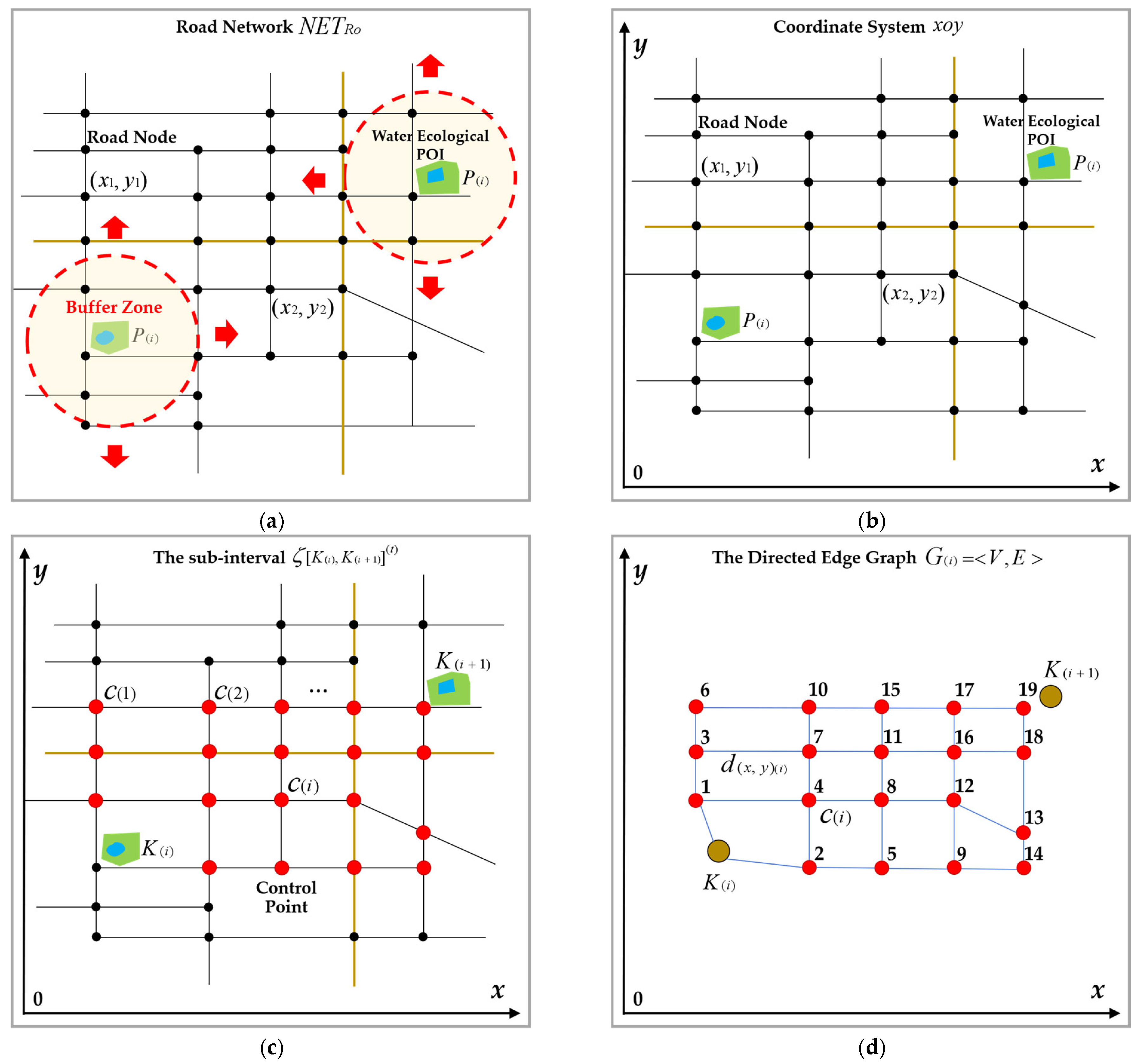
Figure 6 shows the process of constructing the sub-interval coordinate system $xoy$, sub-intervals ${{\zeta }_{[K_{(i)},K_{(i+1)}]}}^{(t)}$, and the directed weighted edge graph $G_{(i)}$ between the urban water ecological POIs by the ${NET}_{Ro}$. Figure 6a shows the road network, road nodes, and the constructed ${NET}_{Ro}$ within the buffer zone of POIs; Figure 6b shows the constructed coordinate system $xoy$ for ${NET}_{Ro}$ based on Figure 6a; Figure 6c shows the process of selecting the key control points $C_{(i)}$ from the coordinate system $xoy$, determining $K_{(i)}$ and $K_{(i+1)}$ to form the sub-interval ${{\zeta }_{[K_{(i)},K_{(i+1)}]}}^{(t)}$; Figure 6d shows the directed weighted edge graph $G_{(i)}=<V,E>$ and sub-interval ${{\zeta }_{[K_{(i)},K_{(i+1)}]}}^{(t)}$.

According to the directional features of the logistics routes, the process of the vehicles moving from the starting point of the water ecological POI $K_{(i)}$ to the endpoint of the water ecological POI $K_{(i+1)}$ has the feature of one-way non-turning. Therefore, the process of constructing the simulated Huffman spatial searching tree (SHSST) takes the direction of the vehicle movement as the node searching direction, and the route does not turn back. We stipulate the following:

(1) The parent node of SHSST is the starting point $K_{(i)}$, the highest level node is the endpoint $K_{(i+1)}$, and the tree node is the key control point $C_{(i)}$.

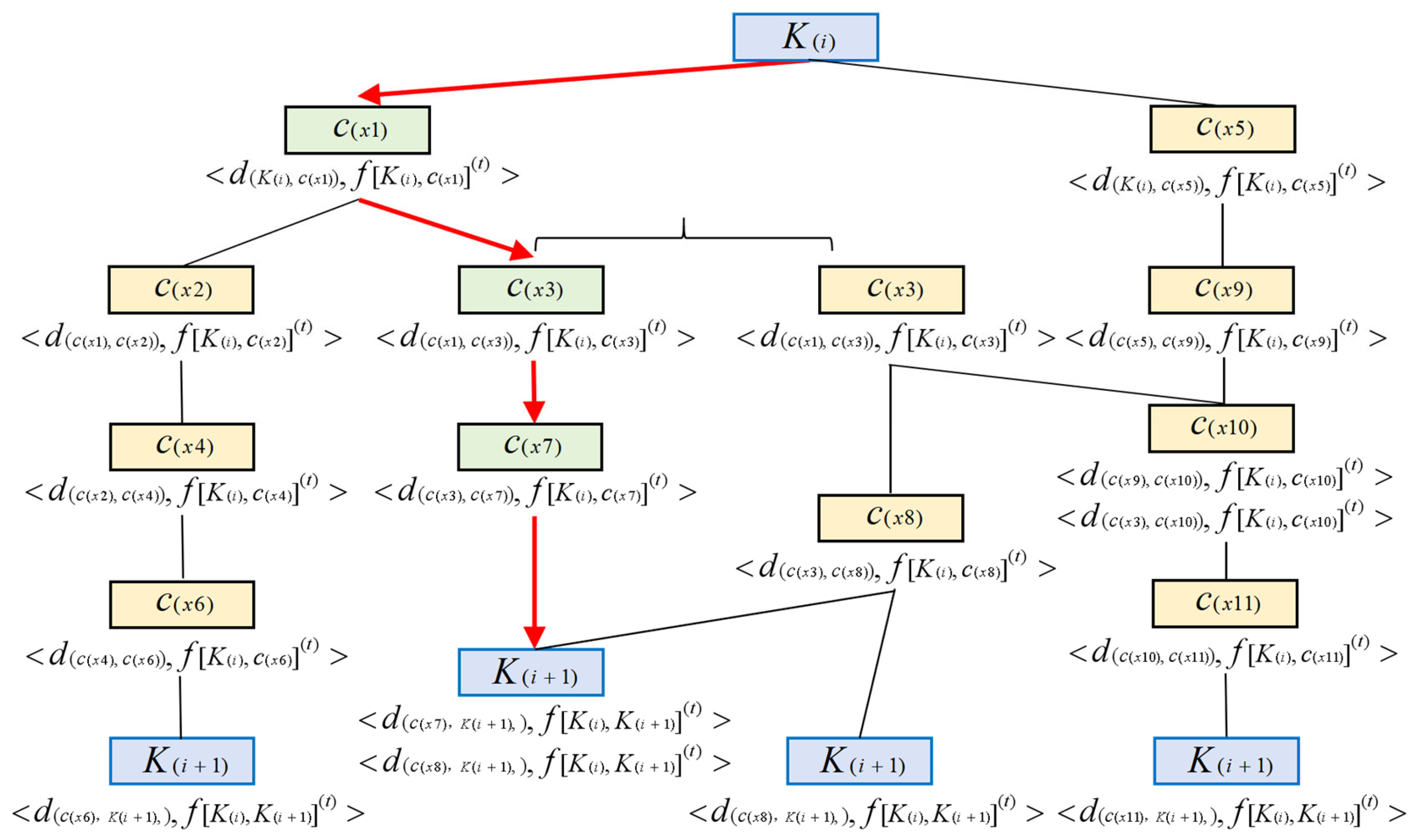
(2) The tree node storage structure is < $d_{{(x,y)}_{(i)}}$, ${f_{[K_{(i)},c_{(i)}]}}^{(t)}$>, in which $d_{{(x,y)}_{(i)}}$ is the edge weight between the current node $C_{(i)}$ and the previous node $c_{(i-1)}$, and ${f_{[K_{(i)},c_{(i)}]}}^{(t)}$ is the total weight of the current searched path when SHSST searches to the node $C_{(i)}$.

(3) At the end of the search for SHSST, it contains multiple feasible paths. The minimum value of the highest-level node ${f_{[K_{(i)},K_{(i+1)}]}}^{(t)}$ is searched, and the path that connects the minimum value is the shortest path in the sub-interval ${{\zeta }_{[K_{(i)},K_{(i+1)}]}}^{(t)}$.

Suppose that the List $C_{losed}$ represents the set of points in the control point set $\left\{c_{(i)}\right\}$ that have been searched and have a determined distance to the starting point $K_{(i)}$, and the List $O_{pen}$ represents the set of points in the control point set $\left\{c_{(i)}\right\}$ that have not been determined to have a distance to the starting point $K_{(i)}$, then there is $C_{losed}\subset \left\{c_{(i)}\right\}$, $O_{pen}\subset \left\{c_{(i)}\right\}$. The cost ${f_{[K_{(i)},c_{(i)}]}}^{(t)}$ of the current searching state from the starting point $K_{(i)}$ to the control points $C_{(i)}$ in the set $\left\{c_{(i)}\right\}$ is defined as the cost of the shortest path that starts from the starting point $K_{(i)}$ and passes through the control points in the List $C_{losed}$, but directly arrives $C_{(i)}$ without passing through the control points in the List $O_{pen}$. For all control points $C_{(i)}$ in the set $\left\{c_{(i)}\right\}$, if there is a weight edge of a connected path from the starting point $K_{(i)}$ to the current searching point $C_{(i)}$, then there is ${f_{[K_{(i)},c_{(i)}]}}^{(t)}\propto {\displaystyle {\sum }_{i=1}^{\max i}{d}_{{(x,y)}_{(i)}}}$, otherwise, ${f_{[K_{(i)},c_{(i)}]}}^{(t)}=\infty$ is specified. For the set $\left\{c_{(i)}\right\}$ of all control points $C_{(i)}$, search for the point that makes the ${f_{[K_{(i)},c_{(i)}]}}^{(t)}$ minimum:

$${f_{[K_{(i)},c_{(i)}]}}^{(t)}=\min \left\{{f_{[K_{(i)},c_{(x)}]}}^{(t)}|\in \{{\mathsf{C}}_{\left(i\right)}\}\right\}$$

(12)

In Formula (12), ${f_{[K_{(i)},c_{(i)}]}}^{(t)}$ is the minimum cost obtained by the searching from the starting point $K_{(i)}$ to $C_{(i)}$, and $C_{(i)}$ is currently the closest point in the set $\left\{c_{(i)}\right\}$ to $K_{(i)}$. Remove $C_{(i)}$ from $\left\{c_{(i)}\right\}$ and store it in the List $C_{losed}$. For all other points $c_{(x)}$ in the set $\left\{c_{(i)}\right\}$ that are adjacent to the current one $C_{(i)}$, iteratively update ${f_{[K_{(i)},c_{(i)}]}}^{(t)}$ according to Formula (13) until they satisfy $C_{losed}=\left\{c_{(i)}\right\}$ and $O_{pen}=\varnothing$.

$${f_{[K_{(i)},c_{(i)}]}}^{(t)}=\min \{{f_{[K_{(i)},c_{(i)}]}}^{(t)},{f_{[K_{(i)},c_{(x)}]}}^{(t)}\}$$

(13)

According to the SHSST modeling principle, we construct the sub-interval optimal route-searching algorithm based on the symmetrical simulated Huffman spatial searching tree as follows:

Step 1: In the graph $g_{(i)}=<V,E>$, set $c_{(x)}$ as the previous point in the shortest path from the starting point $K_{(i)}$ to the point $C_{(i)}$, and $V$ is the set containing points $K_{(i)}$, $K_{(i+1)}$, and $C_{(i)}$ in the SHSST. Initialize $C_{losed}=\left\{K_{(i)}\right\}$, $O_{pen}=V-\left\{K_{(i)}\right\}$.

Step 2: For any $\forall c_{(x)}\in O_{pen}$, if there is $K_{(i)},c_{(x)}\in \mathrm{SHSST}$, then there must be the following: ${f_{[K_{(i)},c_{(x)}]}}^{(t)}\propto {\displaystyle {\sum }_{i=1}^{\max i}{d}_{(x,y)(i)}}$, $c_{(x)}=K_{(i)}$; Otherwise, ${f_{[K_{(i)},c_{(x)}]}}^{(t)}=\infty$, $c_{(x)}=-1$.

Step 3: Search $c_{(r)}\in O_{pen}$, so that ${f_{[K_{(i)},c_{(i)}]}}^{(t)}={{\min \{f}_{[K_{(i)},c_{(i)}]}}^{(t)}| x\in \{c_{(i)}\}\}$, then the ${f_{[K_{(i)},c_{(i)}]}}^{(t)}$ is the minimum cost from $c_{(r)}$ to $K_{(i)}$.

Step 4: Update $C_{losed}=C_{losed}\cup \left\{c_{(r)}\right\}$, $O_{pen}=O_{pen}-\left\{c_{(r)}\right\}$.

Step 5: If $O_{pen}=\varnothing$, the algorithm ends; Otherwise, turn to Step 6.

Step 6: For all the adjacent points $c_{(x)}$ to $c_{(r)}$, if they satisfy ${f_{[K_{(i)},c_{(x)}]}}^{(t1)}\le {f_{[K_{(i)},c_{(x)}]}}^{(t2)}$, in which ${f_{[K_{(i)},c_{(x)}]}}^{(t2)}$ satisfies the Formula (14), $\delta$ is the dimensionality reduction parameter, the ${f_{[K_{(i)},c_{(x)}]}}^{(t1)}$ is the cost from $K_{(i)}$ to $c_{(x)}$, the ${f_{[K_{(i)},c_{(x)}]}}^{(t2)}$ is the cost from $K_{(i)}$ to $c_{(r)}$ adding the cost from $c_{(r)}$ to $c_{(x)}$, then turn to Step 3; Otherwise, for the points $c_{(x)}$ that are not satisfied, set ${f_{[K_{(i)},c_{(x)}]}}^{(t1)}={f_{[K_{(i)},c_{(x)}]}}^{(t2)}$, $c_{(x)}=c_{(r)}$, and turn to Step 3.

$${f_{[K_{(i)},c_{(x)}]}}^{(t2)}=\delta \times \left[d_{{(c_{(r)},c_{(x)})}_{(i)}}+{\displaystyle \sum _{i=1}^{\max i}{d}_{{(x,y)}_{(i)}}}\right]$$

(14)

According to the algorithm modeling process, construct the symmetrical simulated Huffman spatial searching tree model, SHSST, as shown in Figure 7, in which each node represents a sub-interval control point $C_{(i)}$ and the connecting edges of the tree are logistics paths. The red path in the Figure 7 is an example of the optimal path in the sub-interval.

3.3.2. Global Logistics Route-Planning Algorithm Based on Undirected Complete Graph Spatial Search

On the basis of constructing the sub-interval SHSST model, we determine the logistics path ${{\zeta }_{[K_{(i)},K_{(i+1)}]}}^{(t)}$ with the minimum cost ${f_{[K_{(i)},K_{(i+1)}]}}^{(t)}$ for each sub-interval. The logistics vehicle starts from the departure point $K_{(i)}$, completes the material distribution of $n$ number of water ecological POIs, and finally returns to the destination $K_{(i)}$, forming a closed logistics route. The closed route contains $n+1$ number of sub-intervals ${{\zeta }_{[K_{(i)},K_{(i+1)}]}}^{(t)}$. In non-emergency situations, due to the disorderliness of the logistics distribution, the logistics vehicles show the feature of disorderliness in the material distribution to the $n$ number of water ecological POIs. That is, when the distribution order changes, the logistics route and cost also change accordingly [33,34]. Based on this characteristic, we construct the global logistics route-planning algorithm based on the undirected complete graph spatial search.

Specifically, the logistics vehicle starts from the departure point $D_{(i)}$, passes through $n$ number of water ecological POI nodes $P_{(i)}$ for material distribution, and finally returns to the destination $D_{(i)}$. The complete route formed by this process is the logistics route interval ${L_{[D_{(i)},D_{(i)}]}}^{(u)}$, in which $u$ represents the No. $u$ type of interval. Construct a $1\times (n+2)$ dimension logistics route interval vector ${L_{[D_{(i)},D_{(i)}]}}^{(u)}$ for storing logistics route nodes $K_{(i)}$, in which $u$ represents the No. $u$ type of vector. The vector ${L_{[D_{(i)},D_{(i)}]}}^{(u)}$ contains $n+2$ number of elements, with No. $i$ element specified as $L_{(i)}$. The elements $L_{(1)}$ and $L_{(n+2)}$ store $D_{(i)}$, and $L_{(2)}$~$L_{(n+1)}$ store POIs $P_{(i)}$.

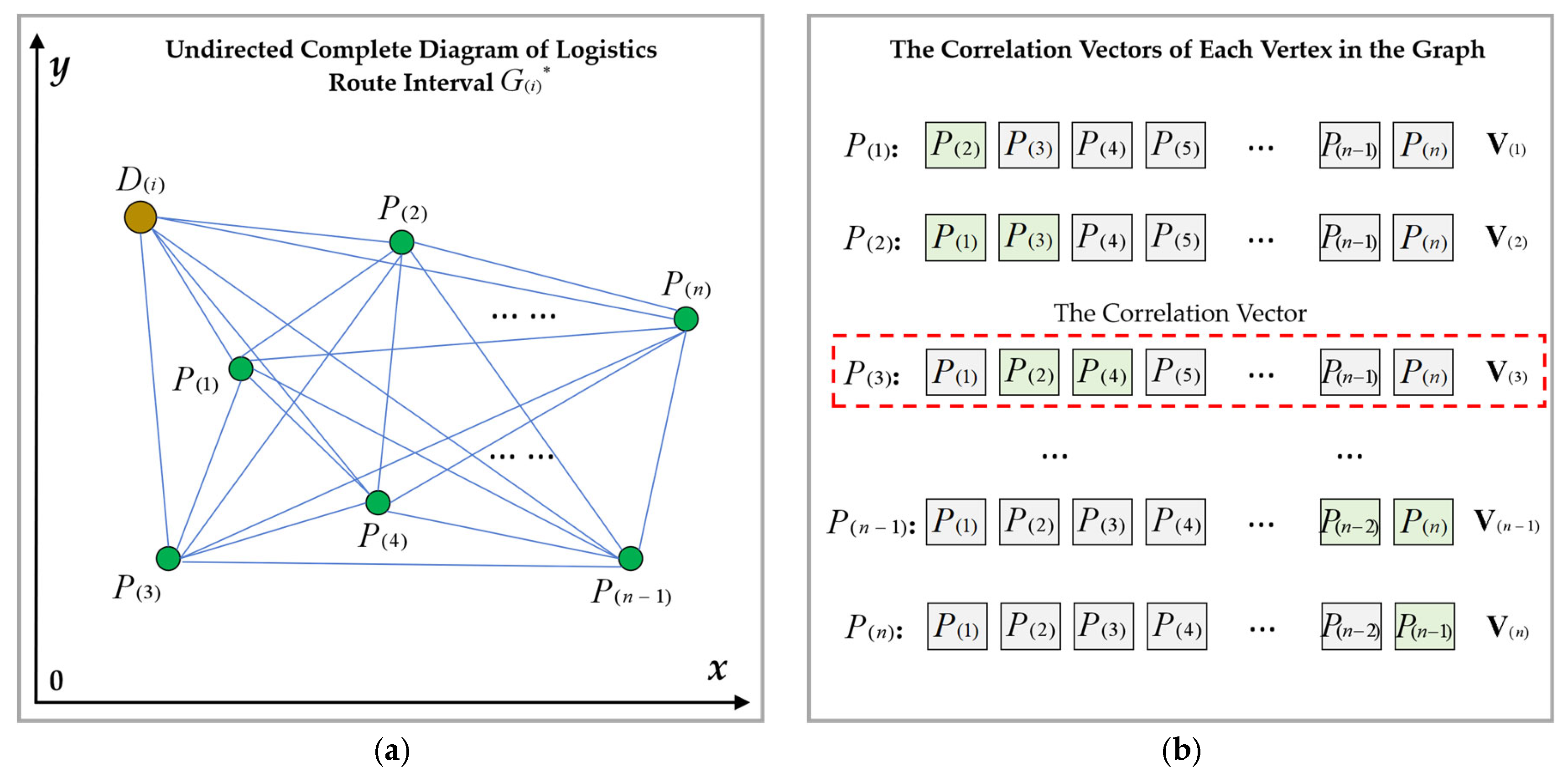
According to the disorderliness of the logistics distribution, the logistics route intervals have the undirected features, including $n+2$ number of nodes and $n+1$ number of sub-intervals ${{\zeta }_{[K_{(i)},K_{(i+1)}]}}^{(t)}$. Construct a graph containing $n+2$ number of vertices and $C(n+2,2)$ number of undirected edges, with each vertex connected to the other $n+1$ number of vertices, which forms an undirected complete graph, denoted as ${G_{(i)}}^{*}=<V,E>$. Discretize the graph ${G_{(i)}}^{*}$. For any vertex $V_{(i)}$ of ${G_{(i)}}^{*}$, a $1\times (n+1)$ dimension vector $V_{(i)}$ is constructed by connecting the remaining $n+1$ number of vertices through the undirected weighted edges. Its elements store the remaining $n+1$ number of vertices, and the vector is the discrete correlation vector of the graph ${G_{(i)}}^{*}$. Set the vector element as $V_{(i,j)}$, $0<j\le n+1$, $j,n\in N$. Figure 8a shows the undirected complete graph ${G_{(i)}}^{*}$, and Figure 8b is the example of the correlation vectors of each vertex obtained after the discretization of graph ${G_{(i)}}^{*}$.

Based on the vector ${L_{[D_{(i)},D_{(i)}]}}^{(u)}$ and the sub-interval cost ${f_{[K_{(i)},K_{(i+1)}]}}^{(t)}$, the logistics interval cost function ${f_{[D_{(i)},D_{(i)}]}}^{(u)}$ is constructed as Formula (15), in which the $u$ represents the No. $u$ kind of vector. It represents the different generated route directions when the logistics sequence changes. Based on the $n$ number of logistics distribution POI nodes $P_{(i)}$ and possible types of routes, it meets $0<u\le A(n,n)$, $u,n\in N$.

$${f_{[D_{(i)},D_{(i)}]}}^{(u)}={\displaystyle \frac{1}{{\displaystyle \sum _{t=1}^{n+1}{f_{[K_{(i)},K_{(i+1)}]}}^{(t)}}}}$$

(15)

Based on the number $u$ of the logistics intervals ${L_{[D_{(i)},D_{(i)}]}}^{(u)}$ output by the iteration, we calculate $A(n,n)$ number of the cost functions ${f_{[D_{(i)},D_{(i)}]}}^{(u)}$ for the logistics intervals, then construct the logistics cost complete binary tree $T_{f_{(u)}}$ with $A(n,n)$ number of nodes to store ${f_{[D_{(i)},D_{(i)}]}}^{(u)}$.

We construct the global logistics route-planning algorithm based on the undirected complete graph spatial search. Figure 9 shows the flowchart of the constructed algorithm.

Step 1: Build a logistics cost complete binary tree $T_{f_{(u)}}$ containing $A(n,n)$ number of nodes. Set $u=1$, initialize ${L_{[D_{(i)},D_{(i)}]}}^{(u)}$, and establish the first vector ${L_{[D_{(i)},D_{(i)}]}}^{(1)}$. Store the selected starting and ending points $D_{(i)}$ in the element $L_{(1)}$ and $L_{(n+2)}$.

Step 2: Store $n$ number of water ecological POI nodes $P_{(i)}$ to elements $L_{(2)}$~$L_{(n+1)}$.

(1) Initialize $n$ number of correlation vectors $V_{(i)}$: $V_{(1)}$~$V_{(n)}$ for $P_{(i)}$.

(2) In $V_{(1)}$, randomly select the arbitrary element ${\forall V}_{(1,j)}$~$P_{(i)}$ and store it as an element $L_{(2)}$ in the vector ${L_{[D_{(i)},D_{(i)}]}}^{(1)}$.

(3) In $V_{(2)}$, randomly select the arbitrary element ${\forall V}_{(2,j)}$~$P_{(i)}$ and determine the following:

① If $V_{(1,j)}\ne V_{(2,j)}$, store $V_{(2,j)}$~$P_{(i)}$ into the element $L_{(3)}$ of the vector ${L_{[D_{(i)},D_{(i)}]}}^{(1)}$.

② If $V_{(1,j)}=V_{(2,j)}$, delete $V_{(2,j)}$, return to Step (3) to select $V_{(2,j)}$ and judge until the selected $V_{(2,j)}$ meets condition ①, and then store it in the element $L_{(3)}$.

(4) According to the method in Step (3), randomly select an arbitrary element $\forall V_{(i,j)}$~$P_{(i)}$ from $V_{(i)}$, $V_{(i)}:2<i\le n$, and determine the following:

① If $V_{(i,j)}\ne {\forall V}_{(x,j)}$, then among them the $x$ traverses $0<x\le i-1$. Store $V_{(i,j)}$~$P_{(i)}$ into the element $L_{(i+1)}$ of the vector ${L_{[D_{(i)},D_{(i)}]}}^{(1)}$.

② If $V_{(i,j)}={\forall V}_{(x,j)}$, delete $V_{(i,j)}$, return to Step (4) to select $V_{(i,j)}$ and judge until the selected $V_{(i,j)}$ meets condition ①, and then store it in the element $L_{(i+1)}$.

(5) Repeat Step (4) until the vector $V_{(n)}$ search is complete. Store the elements $V_{(n,j)}$ that meet the conditions into $L_{(n+1)}$. The vector ${L_{[D_{(i)},D_{(i)}]}}^{(1)}$ storage is completed.

Step 3: Based on the vector ${L_{[D_{(i)},D_{(i)}]}}^{(1)}$ and the element $L_{(i)}$ storage structure, search for $n+1$ number of sub-intervals ${{\zeta }_{[K_{(i)},K_{(i+1)}]}}^{(t)}$ consisting of $n+2$ number of nodes $K_{(i)}$. Determine the cost value ${f_{[K_{(i)},K_{(i+1)}]}}^{(t)}$ of each sub-interval ${{\zeta }_{[K_{(i)},K_{(i+1)}]}}^{(t)}$ and calculate to output the interval cost value ${f_{[D_{(i)},D_{(i)}]}}^{(1)}$.

Step 4: Return to the Step 1, set $u=2$, initialize ${L_{[D_{(i)},D_{(i)}]}}^{(u)}$, and set up the second vector ${L_{[D_{(i)},D_{(i)}]}}^{(2)}$.

(1) Store $n$ number of water ecological POI nodes $P_{(i)}$ to elements $L_{(2)}$~$L_{(n+1)}$.

(2) Based on the vector ${L_{[D_{(i)},D_{(i)}]}}^{(2)}$ and the element $L_{(i)}$ storage structure, search for $n+1$ number of sub-intervals ${{\zeta }_{[K_{(i)},K_{(i+1)}]}}^{(t)}$ consisting of $n+2$ number of nodes $K_{(i)}$.

(3) Determine the cost value ${f_{[K_{(i)},K_{(i+1)}]}}^{(t)}$ of each sub-interval ${{\zeta }_{[K_{(i)},K_{(i+1)}]}}^{(t)}$ and calculate to output the interval cost value ${f_{[D_{(i)},D_{(i)}]}}^{(2)}$.

Step 5: According to the algorithm from the Step 3 to Step 4, for any $\forall u$, initialize the ${L_{[D_{(i)},D_{(i)}]}}^{(u)}$ and establish the No. $u$ vector ${L_{[D_{(i)},D_{(i)}]}}^{(u)}$, and calculate to output interval cost ${f_{[D_{(i)},D_{(i)}]}}^{(u)}$. Traverse $2<u\le A(n,n)$ and output $A(n,n)$ number of cost values ${f_{[D_{(i)},D_{(i)}]}}^{(u)}$ of the logistics intervals ${L_{[D_{(i)},D_{(i)}]}}^{(u)}$.

Step 6: Store $A(n,n)$ number of cost values ${f_{[D_{(i)},D_{(i)}]}}^{(u)}$ to the complete binary tree $T_{f_{(u)}}$.

(1) Take ${f_{[D_{(i)},D_{(i)}]}}^{(1)}$ and ${f_{[D_{(i)},D_{(i)}]}}^{(2)}$ and compare the following:

① If ${f_{[D_{(i)},D_{(i)}]}}^{(1)}\ge {f_{[D_{(i)},D_{(i)}]}}^{(2)}$, store ${f_{[D_{(i)},D_{(i)}]}}^{(1)}$ to the parent node ${N_{ode}}_{(0,1)}$ and store ${f_{[D_{(i)},D_{(i)}]}}^{(2)}$ to the child node ${N_{ode}}_{(1,1)}$.

② If ${f_{[D_{(i)},D_{(i)}]}}^{(1)}<{f_{[D_{(i)},D_{(i)}]}}^{(2)}$, store ${f_{[D_{(i)},D_{(i)}]}}^{(2)}$ to the parent node ${N_{ode}}_{(0,1)}$ and store ${f_{[D_{(i)},D_{(i)}]}}^{(1)}$ to the child node ${N_{ode}}_{(1,1)}$.

(2) Take ${f_{[D_{(i)},D_{(i)}]}}^{(3)}$, and further compare the following:

① If ${f_{[D_{(i)},D_{(i)}]}}^{(1)}\ge {f_{[D_{(i)},D_{(i)}]}}^{(2)}$:

(i) If ${f_{[D_{(i)},D_{(i)}]}}^{(3)}\ge {f_{[D_{(i)},D_{(i)}]}}^{(1)}\ge {f_{[D_{(i)},D_{(i)}]}}^{(2)}$, store ${f_{[D_{(i)},D_{(i)}]}}^{(3)}$, ${f_{[D_{(i)},D_{(i)}]}}^{(1)}$, and ${f_{[D_{(i)},D_{(i)}]}}^{(2)}$ to the parent node ${N_{ode}}_{(0,1)}$, child node ${N_{ode}}_{(1,1)}$, and ${N_{ode}}_{(1,2)}$.

(ii) If ${f_{[D_{(i)},D_{(i)}]}}^{(1)}>{f_{[D_{(i)},D_{(i)}]}}^{(3)}\ge {f_{[D_{(i)},D_{(i)}]}}^{(2)}$, store ${f_{[D_{(i)},D_{(i)}]}}^{(1)}$, ${f_{[D_{(i)},D_{(i)}]}}^{(3)}$, and ${f_{[D_{(i)},D_{(i)}]}}^{(2)}$ to the parent node ${N_{ode}}_{(0,1)}$, child node ${N_{ode}}_{(1,1)}$, and ${N_{ode}}_{(1,2)}$.

(iii) If ${f_{[D_{(i)},D_{(i)}]}}^{(1)}\ge {f_{[D_{(i)},D_{(i)}]}}^{(2)}\ge {f_{[D_{(i)},D_{(i)}]}}^{(3)}$, store ${f_{[D_{(i)},D_{(i)}]}}^{(1)}$, ${f_{[D_{(i)},D_{(i)}]}}^{(2)}$, and ${f_{[D_{(i)},D_{(i)}]}}^{(3)}$ to the parent node ${N_{ode}}_{(0,1)}$, child node ${N_{ode}}_{(1,1)}$, and ${N_{ode}}_{(1,2)}$.

② If ${f_{[D_{(i)},D_{(i)}]}}^{(1)}<{f_{[D_{(i)},D_{(i)}]}}^{(2)}$:

(i) If ${f_{[D_{(i)},D_{(i)}]}}^{(1)}<{f_{[D_{(i)},D_{(i)}]}}^{(2)}\le {f_{[D_{(i)},D_{(i)}]}}^{(3)}$, store ${f_{[D_{(i)},D_{(i)}]}}^{(3)}$, ${f_{[D_{(i)},D_{(i)}]}}^{(2)}$, and ${f_{[D_{(i)},D_{(i)}]}}^{(1)}$ to the parent node ${N_{ode}}_{(0,1)}$, child node ${N_{ode}}_{(1,1)}$, and ${N_{ode}}_{(1,2)}$.

(ii) If ${f_{[D_{(i)},D_{(i)}]}}^{(1)}<{f_{[D_{(i)},D_{(i)}]}}^{(3)}<{f_{[D_{(i)},D_{(i)}]}}^{(2)}$, store ${f_{[D_{(i)},D_{(i)}]}}^{(2)}$, ${f_{[D_{(i)},D_{(i)}]}}^{(3)}$, and ${f_{[D_{(i)},D_{(i)}]}}^{(1)}$ to the parent node ${N_{ode}}_{(0,1)}$, child node ${N_{ode}}_{(1,1)}$, and ${N_{ode}}_{(1,2)}$.

(iii) If ${f_{[D_{(i)},D_{(i)}]}}^{(3)}\le {f_{[D_{(i)},D_{(i)}]}}^{(1)}<{f_{[D_{(i)},D_{(i)}]}}^{(2)}$, store ${f_{[D_{(i)},D_{(i)}]}}^{(2)}$, ${f_{[D_{(i)},D_{(i)}]}}^{(1)}$, and ${f_{[D_{(i)},D_{(i)}]}}^{(3)}$ to the parent node ${N_{ode}}_{(0,1)}$, child node ${N_{ode}}_{(1,1)}$, and ${N_{ode}}_{(1,2)}$.

(4) Repeat the above steps, take ${f_{[D_{(i)},D_{(i)}]}}^{(1)}$, ${f_{[D_{(i)},D_{(i)}]}}^{(2)}$,…, ${f_{[D_{(i)},D_{(i)}]}}^{(j)}$ and make the comparison. According to the binary tree $T_{f_{(u)}}$ storage rules, store the elements ${f_{[D_{(i)},D_{(i)}]}}^{(j)}$ to each node $N_{ode(i,j)}$ of the binary tree.

(5) For ${f_{[D_{(i)},D_{(i)}]}}^{(j)}$, when the traversal $j=A(n,n)$ is complete, the binary tree $T_{f_{(u)}}$ completes the storage and forms the largest tree.

Step 7: For the output complete binary tree $T_{f_{(u)}}$, select the parent node ${N_{ode}}_{(0,1)}$ whose stored ${f_{[D_{(i)},D_{(i)}]}}^{(j)}$ corresponding to vector ${L_{[D_{(i)},D_{(i)}]}}^{(u)}$ is the optimal logistics route with the lowest cost and pollutant emissions.

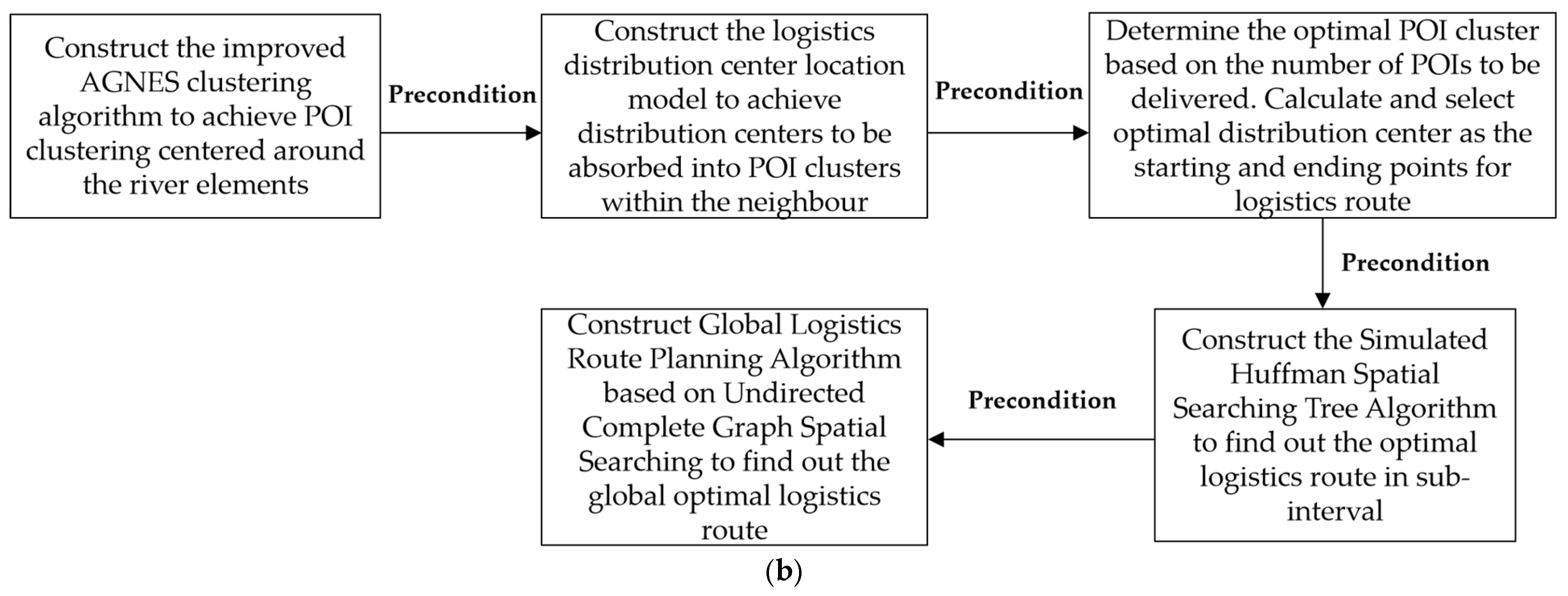
4. Experimental Results and Analysis

To verify the feasibility and advantages of the constructed algorithm model, we designed a sample experiment to validate the constructed algorithm model. At the same time, we designed a comparative experiment to compare the constructed route-planning algorithm with the commonly used route-searching algorithms in logistics planning and obtained relevant conclusions.

4.1. Data Collection

In China, many tourist cities have a good water ecological environment and many water ecological POIs, whose tourism theme focuses on water ecology and water sightseeing. Chengdu, as the capital city of Sichuan Province in China, is well-known for the “park city under the snow-capped mountains”. It is rich in water resources, with a network of rivers, lakes, reservoirs, and other water areas amounting to 943 square kilometers, and accounting for around 6.4% of the city’s total area. There are abundant water tourism destinations in Chengdu, including urban rivers, wetland parks, reservoirs, lakes, etc. The ecological environment of water resource POIs is fragile and highly susceptible to human activities, and it is necessary to reduce the damage caused by human activities. We take the main urban area of Chengdu as the research scope, with the goal of water ecological POI material distribution. We construct a coordinate system $xoy$ for the geospatial scope of Chengdu and establish the main road network ${NET}_{Ro}$ and main water network meta-structure $WMS$. Then, we collect the representative water ecological POIs and their coordinates, and we also collect the corresponding cluster control point sets $C_{on(i)}$ of $WMS$ as well as their coordinates. From the perspective of fairness in the distribution of logistics distribution centers, we select several logistics centers $D_{(i)}$ and determine their coordinates. Then, we construct the logistics sub-intervals and logistics intervals based on the optimal distribution center output by the algorithm as the starting and ending points, and use the POIs to be delivered as nodes, finally output the optimal logistics route. Finally, a comparative experiment is designed with the same sub-intervals and intervals as experimental conditions to compare the route costs between the control group and the experimental group.

(1) The collected ${NET}_{Ro}$ and $WMS$.

Based on the geospatial data and water resource distribution data of Chengdu city, we first select the water spatial scope of Chengdu city, as shown in Figure 10a, including main roads, major river networks, etc. Then, in the water spatial area, we use the main road data as the structure and set up ${NET}_{Ro}$, as Figure 10b shows. We collect four representative rivers from the main water network structure in the urban area of Chengdu city, namely “Fu He River”, “Modi He River”, “Qingshui He River”, and “Nan He River”. All four rivers are natural rivers (non-artificial canals) that flow through the urban area of Chengdu city. Then, we use the confluence points of the four rivers as boundaries to divide the rivers into different sections and establish $WMS$ and the river projection dataset $W$, with different colors representing different dataset elements $W_{(i)}$, as shown in Figure 10c. The initial buffer zone of the water ecological POI cluster $C_{(i)}$ is obtained from the spatial distribution of elements $W_{(i)}$, as shown in Figure 10d, in which different colored planar regions represent the initial buffer zones; after overlaying ${NET}_{Ro}$ and $WMS$, Figure 10e is obtained, which includes each element $W_{(i)}$ and the generated control points $C_{on(i,j)}$. Obtain the cluster control point set $C_{on(i)}$ by overlaying ${NET}_{Ro}$ and $WMS$ as shown in Figure 10e,f.

(2) The collected coordinates of water ecological POIs $P_{(i)}$ and cluster control points $C_{on(i,j)}$.

We collect the water ecological POIs and coordinates in Chengdu city, as shown in

Table 1. The collected water ecological POIs and coordinates in Chengdu city.

$P_{(i)}$	$P_{(1)}$	$P_{(2)}$	$P_{(3)}$	$P_{(4)}$	$P_{(5)}$	$P_{(6)}$
$x_{P_{(i)}}$	104.057	104.105	104.095	104.087	104.036	104.027
$y_{P_{(i)}}$	30.657	30.656	30.667	30.616	30.628	30.657
$P_{(i)}$	$P_{(7)}$	$P_{(8)}$	$P_{(9)}$	$P_{(10)}$	$P_{(11)}$	$P_{(12)}$
$x_{P_{(i)}}$	104.094	104.047	104.092	104.072	104.056	104.029
$y_{P_{(i)}}$	30.686	30.646	30.629	30.675	30.691	30.675

, in which each POI is as follows: {$P_{(1)}$: The People’s Park; $P_{(2)}$: The Xinhua Park; $P_{(3)}$: The Chenghua Park; $P_{(4)}$: The Donghu Park; $P_{(5)}$: The Lidu Park; $P_{(6)}$: The Huanhuaxi Park; $P_{(7)}$: The Sandong Guqiao Park; $P_{(8)}$: The Wuhou Temple; $P_{(9)}$: The Wangjianglou Park; $P_{(10)}$: The Wenshu Monastery; $P_{(11)}$: The Jiulidi Park; and $P_{(12)}$: The Shiren Park}. The coordinates of the control points $C_{on(i,j)}$ are shown in

Table 2. The collected cluster control points and their coordinates.

	$C_{on(1)}$
	$C_{on(1,1)}$			$C_{on(1,2)}$			$C_{on(1,3)}$			$C_{on(1,4)}$			$C_{on(1,5)}$			$C_{on(1,6)}$
$x_{C_{on(i,j)}}$	104.060			104.060			104.064			104.071			104.078			104.084
$y_{C_{on(i,j)}}$	30.694			30.685			30.682			30.678			30.675			30.672
	$C_{on(4)}$
	$C_{on(4,1)}$		$C_{on(4,2)}$			$C_{on(4,3)}$		$C_{on(4,4)}$				$C_{on(4,5)}$		$C_{on(4,6)}$			$C_{on(4,7)}$
$x_{C_{on(i,j)}}$	104.022		104.041			104.047		104.056				104.060		104.066			104.074
$y_{C_{on(i,j)}}$	30.65		30.656			30.651		30.648				30.647		30.646			30.645
	$C_{on(2)}$						$C_{on(3)}$						$C_{on(5)}$
	$C_{on(2,1)}$	$C_{on(2,2)}$			$C_{on(2,3)}$		$C_{on(3,1)}$		$C_{on(3,2)}$		$C_{on(3,3)}$		$C_{on(5,1)}$		$C_{on(5,2)}$			$C_{on(5,3)}$
$x_{C_{on(i,j)}}$	104.091	104.088			104.085		104.029		104.039		104.036		104.089		104.092			104.085
$y_{C_{on(i,j)}}$	30.661	30.653			30.648		30.680		30.667		30.661		30.639		30.635			30.620

.

(3) The collected logistics distribution centers $D_{(i)}$ and coordinates $x_{D_{(i)}}$ and $y_{D_{(i)}}$

Set the large shopping malls, wholesale markets, etc., as the material distribution centers. We collected the distribution centers, and their coordinates in Chengdu city are shown in

Table 3. The collected distribution centers and their coordinates.

${\mathit{D}}_{(\mathit{i})}$	${\mathit{D}}_{(1)}$	${\mathit{D}}_{(2)}$	${\mathit{D}}_{(3)}$	${\mathit{D}}_{(4)}$	${\mathit{D}}_{(5)}$	${\mathit{D}}_{(6)}$	${\mathit{D}}_{(7)}$	${\mathit{D}}_{(8)}$
$x_{P_{(i)}}$	104.067	104.074	104.078	104.115	104.020	104.057	104.094	104.021
$y_{P_{(i)}}$	30.631	30.686	30.658	30.649	30.646	30.673	30.677	30.663

, among which the distribution centers are as follows: {$D_{(1)}$: Raffles Mall; $D_{(2)}$: Jinniu Wanda; $D_{(3)}$: Wangfujing, Zongfu Road; $D_{(4)}$: The mixc Mall; $D_{(5)}$: Ito Yokado; $D_{(6)}$: New City Plaza; $D_{(7)}$: Fortune City; and $D_{(8)}$: Maoye Renhe Spring Department Store}. Figure 11 shows the spatial relationship between the collected water ecological POIs, distribution centers, and control points in the urban coordinate system. Figure 11a shows the location projection of water ecological POIs, Figure 11b shows the location projection of distribution centers, Figure 11c shows the location of water ecological POIs, distribution centers, $WMS$, and control points $C_{on(i,j)}$ in the urban geographic space, and Figure 11d shows the spatial relationship structure of the projections on water ecological POIs, distribution centers, $WMS$, and control point $C_{on(i,j)}$.

4.2. Results and Analysis of the Water Ecological POI Spatial Clustering

Using the constructed clustering algorithm, we calculated the objective functions $f_{[P_{(i)},C_{on(i,j)}]}$ for each POI and control point $C_{on(i,j)}$ in the cluster control point set $C_{on(i)}$, and constructed the optimal complete binary tree $T_{W(i)}$ for POI and control point set $C_{on(i)}$ in each cluster. Output the global optimal objective function and the corresponding cluster $C_{(i)}$.

Table 4. The optimal objective function results $f_{[P_{(i)},C_{on(i,j)}]}$ in the parent nodes of the control point sets $C_{on(i)}$ to each POI corresponding to a cluster after constructing the optimal complete binary tree.

	${\mathit{C}}_{(1)}$	${\mathit{C}}_{(2)}$	${\mathit{C}}_{(3)}$	${\mathit{C}}_{(4)}$	${\mathit{C}}_{(5)}$		${\mathit{C}}_{(1)}$	${\mathit{C}}_{(2)}$	${\mathit{C}}_{(3)}$	${\mathit{C}}_{(4)}$	${\mathit{C}}_{(5)}$
$P_{(1)}$	0.400	0.323	0.556	0.769	0.263	$P_{(7)}$	0.556	0.357	0.172	0.204	0.192
$P_{(2)}$	0.357	0.714	0.154	0.323	0.435	$P_{(8)}$	0.238	0.278	0.500	1.667	0.250
$P_{(3)}$	0.769	1.429	0.185	0.333	0.333	$P_{(9)}$	0.204	0.435	0.156	0.400	1.333
$P_{(4)}$	0.159	0.278	0.143	0.286	1.667	$P_{(10)}$	1.667	0.417	0.294	0.313	0.238
$P_{(5)}$	0.156	0.192	0.278	0.370	0.208	$P_{(11)}$	2.000	0.204	0.345	0.238	0.152
$P_{(6)}$	0.238	0.185	1.333	1.053	0.169	$P_{(12)}$	0.323	0.161	1.667	0.435	0.145

shows the optimal objective function results $f_{[P_{(i)},C_{on(i,j)}]}$ in the parent nodes of the control point sets $C_{on(i)}$ to each POI corresponding to cluster after constructing the optimal complete binary tree, in which $C_{on(i)}$ corresponds to the cluster $C_{(i)}$. Figure 12 shows a comparison of the optimal objective functions for the control point sets $C_{on(i)}$ and clusters $C_{(i)}$ corresponding to POIs, in which Figure 12a–l correspond to $P_{(1)}~P_{(12)}$, respectively. According to the calculation results in Table 4 and Figure 12, the clustering results of POIs are as follows: $C_{(1)}$: {$P_{(7)}$, $P_{(10)}$, $P_{(11)}$}; $C_{(2)}$: {$P_{(2)}$, $P_{(3)}$}; $C_{(3)}$: {$P_{(6)}$, $P_{(12)}$}; $C_{(4)}$: {$P_{(1)}$, $P_{(5)}$, $P_{(8)}$}; $C_{(5)}$: {$P_{(4)}$, $P_{(9)}$}.

From the analysis of the calculation results in Table 4 and the objective function bar chart in Figure 12, it can be concluded that the optimal objective function values for each POI relative to the control point set $C_{on(i)}$ and cluster $C_{(i)}$ are different, showing a fluctuating trend. This is determined by the spatial accessibility between POIs and river elements. The higher the spatial accessibility is, the closer the spatial relationship between the POI and the river channel element $W_{(i)}$ will be, and the higher the probability of the POI belonging to the cluster $C_{(i)}$ of the river element $W_{(i)}$ will be. In the Figure 12, the bar charts of arbitrary POI to clusters $C_{(1)}~C_{(5)}$ represent the optimal objective function values of the parent nodes in the complete binary trees $T_{W(i)}$ of the clusters $C_{(i)}$ corresponding to the POI. Among the five optimal objective functions, the objective function with the highest data value is determined, corresponding to the cluster where the POI is located, indicating that the POI has the highest degree of closeness with it. The experiment shows that the proposed algorithm can accurately calculate the closeness value between the POI and the river element $W_{(i)}$ corresponding to the cluster $C_{(i)}$, quantify the relationship between the POI and the cluster $C_{(i)}$, and optimize the clustering results.

According to the analysis of the POI clustering results, the clusters calculated by the clustering algorithm all contain a certain number of POIs, and they are all the calculation results with the maximum objective function value between the POIs and the cluster $C_{(i)}$. The uniform distribution of POIs in each cluster indicates that the algorithm considers the spatial fairness when designing the spatial range of clusters by using the buffer zones, and it takes into account the river flow trends and its uniform distribution throughout the entire spatial range in selecting $WMS$, making the POI dataset fair in calculating the objective function value for each cluster $C_{(i)}$.

4.3. Results and Analysis of the Logistics Route Distribution Center Location

Using the constructed logistics distribution center location model, we calculated the objective functions $f_{[D_{(i)},C_{on(i,j)}]}$ of each distribution center $D_{(i)}$ to cluster the control points $C_{on(i,j)}$ in the set $C_{on(i)}$ separately, and constructed the optimal complete binary tree ${T_{D_{(i)}}}^{[j]}$ of the distribution center $D_{(i)}$ for each cluster control point set $C_{on(i)}$. We output the global optimal objective function and corresponding cluster $C_{(i)}$. Then, we randomly selected the POIs that required the material delivery as $P_{(2)}$: The Xinhua Park; $P_{(5)}$: The Lido Park; $P_{(7)}$: The Sandong Guqiao Park; and $P_{(11)}$: The Jiulidi Park. According to the algorithm, the statistical number of POIs in the cluster $C_{(1)}$ has the maximum value, and therefore, the distribution center set {$D_{(2)}$, $D_{(6)}$, $D_{(7)}$} with the highest correlation to the cluster $C_{(1)}$ is the candidate element set for the optimal distribution center. Finally, we calculated the closeness value $f_{[D_{(i)},P_{(i)}]}$ and the average closeness value ${\overline{f}}_{[D_{(i)},P_{(i)}]}$ between the distribution centers {$D_{(2)}$, $D_{(6)}$, $D_{(7)}$} and the POIs that need a delivery.

Table 5. The optimal objective function results $f_{[D_{(i)},C_{on(i,j)}]}$ in the parent nodes of the control point sets $C_{on(i)}$ corresponding to the clusters $C_{(i)}$ for each distribution center $D_{(i)}$.

	${\mathit{C}}_{(1)}$	${\mathit{C}}_{(2)}$	${\mathit{C}}_{(3)}$	${\mathit{C}}_{(4)}$	${\mathit{C}}_{(5)}$		${\mathit{C}}_{(1)}$	${\mathit{C}}_{(2)}$	${\mathit{C}}_{(3)}$	${\mathit{C}}_{(4)}$	${\mathit{C}}_{(5)}$
$D_{(1)}$	0.208	0.385	0.227	0.588	0.476	$D_{(5)}$	0.175	0.161	0.435	1.333	0.154
$D_{(2)}$	1.042	0.294	0.244	0.222	0.185	$D_{(6)}$	0.909	0.278	0.500	0.417	0.204
$D_{(3)}$	0.588	0.909	0.244	0.667	0.435	$D_{(7)}$	0.833	0.526	0.179	0.244	0.233
$D_{(4)}$	0.250	0.385	0.132	0.256	0.370	$D_{(8)}$	0.213	0.137	0.625	0.833	0.141

shows the optimal objective function results $f_{[D_{(i)},C_{on(i,j)}]}$ in the parent nodes of the control point sets $C_{on(i)}$ corresponding to the clusters $C_{(i)}$ for each distribution center $D_{(i)}$ after constructing the optimal complete binary tree, in which $C_{on(i)}$ corresponds to cluster $C_{(i)}$. Figure 13 shows a comparison of the optimal objective functions for each cluster control point set $C_{on(i)}$ and cluster $C_{(i)}$ corresponding to the distribution center $D_{(i)}$, in which Figure 13a–h corresponds to $D_{(1)}~D_{(8)}$, respectively. According to the calculation results in Table 5 and Figure 13, the closeness relationship between each distribution center $D_{(i)}$ and cluster $C_{(i)}$ is obtained as follows: $C_{(1)}$: {$D_{(2)}$, $D_{(6)}$, $D_{(7)}$}; $C_{(2)}$: {$D_{(3)}$, $D_{(4)}$}; $C_{(3)}$: {$\varnothing$}; $C_{(4)}$: {$D_{(1)}$, $D_{(5)}$, $D_{(8)}$}; $C_{(5)}$: {$\varnothing$}. From the analysis of the calculation results in Table 5 and the objective function bar chart in Figure 13, it can be concluded that the optimal objective function values for each distribution center $D_{(i)}$ to the control point set $C_{on(i)}$ and cluster $C_{(i)}$ are different, showing a fluctuating trend. This is determined by the spatial accessibility between the distribution center $D_{(i)}$ and the river element $W_{(i)}$. The higher the spatial accessibility is, the closer the spatial relationship between the distribution center and the river element $W_{(i)}$ will be, and the higher the probability that the distribution center belongs to the cluster $C_{(i)}$ of the river element $W_{(i)}$ will be. In the Figure, the bar charts of the arbitrary distribution center to clusters $C_{(1)}~C_{(5)}$ represent the optimal objective function values of parent nodes in the complete binary trees ${T_{D(i)}}^{[j]}$ of the clusters $C_{(i)}$ corresponding to the distribution center. Among the five optimal objective functions, the objective function with the highest data value is determined, corresponding to the cluster where the distribution center is located, indicating that the distribution center has the highest degree of closeness with it. The experiment shows that the proposed algorithm can accurately calculate the closeness between the distribution center $D_{(i)}$ and the corresponding cluster $C_{(i)}$ of the river element $W_{(i)}$ and quantify the relationship between the distribution center and the cluster $C_{(i)}$.

Table 6. The closeness values $f_{[D_{(i)},P_{(i)}]}$ and average closeness values ${\overline{f}}_{[D_{(i)},P_{(i)}]}$ between the distribution centers and the POIs to be delivered.

	${\mathit{f}}_{[{\mathit{D}}_{(\mathit{i})},{\mathit{P}}_{(\mathit{i})}]}$				${\overline{\mathit{f}}}_{[{\mathit{D}}_{(\mathit{i})},{\mathit{P}}_{(\mathit{i})}]}$
	${\mathit{P}}_{(2)}$	${\mathit{P}}_{(5)}$	${\mathit{P}}_{(7)}$	${\mathit{P}}_{(11)}$
$D_{(2)}$	0.222	0.135	0.500	0.526	0.346
$D_{(6)}$	0.200	0.185	0.256	0.500	0.285
$D_{(7)}$	0.370	0.127	1.163	0.244	0.476

shows the calculated closeness values $f_{[D_{(i)},P_{(i)}]}$ and the average closeness values ${\overline{f}}_{[D_{(i)},P_{(i)}]}$ between the distribution center {$D_{(2)}$, $D_{(6)}$, $D_{(7)}$} and the POIs that need a delivery. According to the data table, the closeness values between the candidate distribution centers and each POI shows a fluctuating trend. The larger the objective function value is, the higher the closeness will be, and vice versa. The degree of closeness determines the accessibility between the distribution center and POI. The higher the closeness degree is, the higher the accessibility will be, and the lower the costs of logistics sub-interval will be. The average closeness value ${\overline{f}}_{[D_{(i)},P_{(i)}]}$ is the average degree of accessibility between the distribution center and POIs. The higher the average closeness value is, the better the location of the distribution center will be, and the more it can save the overall route costs. According to the calculation results, the average closeness value of the distribution center $D_{(7)}$ is the highest at 0.476, which is the optimal location for the distribution center and is used as the starting and ending points of the logistics route. The experiment proves that the constructed distribution center location algorithm can find out the optimal distribution center based on determining the POIs to be delivered and minimize the spatial layout cost of logistics routes.

4.4. Results and Analysis of the Water Ecological POI Logistics Route

Based on the selected optimal logistics distribution center {$D_{(7)}$: Fortune City} and the POIs to be delivered {$P_{(2)}$: The Xinhua Park; $P_{(5)}$: The Lido Park; $P_{(7)}$: The Sandong Guqiao Bridge Park; and $P_{(11)}$: The Jiulidi Park}, we first listed $D_{(7)}$ and POIs as logistics route nodes $K_{(i)}$ and then constructed logistics sub-intervals ${{\zeta }_{[K_{(i)},K_{(i+1)}]}}^{(t)}$. Search for the control points within the logistics sub-intervals and construct a directed weighted edge graph $G_{(i)}$, determining edge weights $d_{{(x,y)}_{(i)}}$ by the urban geographic information system. Iteratively output the optimal logistics path and the cost function value ${f_{[K_{(i)},K_{(i+1)}]}}^{(t)}$ for each sub-interval with the constructed simulated Huffman spatial searching tree. Secondly, using $D_{(7)}$ and POIs to construct an undirected complete graph ${G_{(i)}}^{*}$, we then introduced the constructed global logistics route-planning algorithm to output the global logistics routes and cost function values ${f_{[D_{(i)},D_{(i)}]}}^{(u)}$.

Table 7. The cost function values ${f_{[K_{(i)},K_{(i+1)}]}}^{(t)}$ of each logistics sub-interval output by the algorithm.

	$D_{(7)}{P}_{(2)}$	$D_{(7)}{P}_{(5)}$	$D_{(7)}{P}_{(7)}$	$D_{(7)}{P}_{(11)}$	$P_{(2)}{P}_{(5)}$
${f_{[K_{(i)},K_{(i+1)}]}}^{(t)}$	0.34	0.97	0.08	0.46	0.88
	$P_{(2)}{P}_{(7)}$	$P_{(2)}{P}_{(11)}$	$P_{(5)}{P}_{(7)}$	$P_{(5)}{P}_{(11)}$	$P_{(7)}{P}_{(11)}$
${f_{[K_{(i)},K_{(i+1)}]}}^{(t)}$	0.4	0.7	0.96	0.85	0.49

shows the cost function values ${f_{[K_{(i)},K_{(i+1)}]}}^{(t)}$ of each logistics sub-interval output by the algorithm, and Figure 14 shows the complete binary tree $Tf(u)$ corresponding to the global logistics routes and cost function values ${f_{[D_{(i)},D_{(i)}]}}^{(u)}$ output by the algorithm. Each node represents a logistics route and cost function, and the symbol $P_{2,5,7,11}$ represents the route $D_{(7)}\to P_{(2)}\to P_{(5)}\to P_{(7)}\to P_{(11)}\to D_{(7)}$. According to the output results in Figure 14, the route $P_{2,5,7,11}$ stored at the parent node $N_{ode(0,1)}$ is the optimal route: $D_{(7)}\to P_{(2)}\to P_{(5)}\to P_{(11)}\to P_{(7)}\to D_{(7)}$; at the same time, the route $P_{7,11,5,2}$ stored in the child node $N_{ode(1,1)}$ is also the optimal route: $D_{(7)}\to P_{(7)}\to P_{(11)}\to P_{(5)}\to P_{(2)}\to D_{(7)}$, and the cost functions of both routes are 0.379. In the complete binary tree $T_{f_{(u)}}$, nodes with higher levels correspond to lower cost function values; on the same level, the cost function corresponding to the left node is greater than that of the right node. The experimental results show that the constructed logistics route-planning algorithm can find out the optimal logistics path and cost function value within the logistics sub-interval, and iteratively output the globally optimal and lowest cost route within the logistics interval, which can effectively reduce the energy consumption and pollutant emissions, and minimize the impact on the water ecological environment and water ecological POIs.

4.5. Results and Analysis of the Comparative Experiment

To verify the advantages of the constructed algorithms, we designed comparative experiments in the same application scenarios. We set the experimental group as the constructed SHSST algorithm (PSA) and the control group as the most commonly used Dijkstra route-searching algorithm and the Prim route-searching algorithm for logistics route planning. The Dijkstra algorithm and Prim algorithm are both algorithms that traverse all vertices of a weighted edge graph, with the goal of minimizing the cost of the route or tree that traverses all vertices. According to the direction of vehicle movement in the logistics sub-intervals and logistics intervals, in order to reduce the cost of the route, it is stipulated that the vehicles do not go back or return. Therefore, when designing the control group algorithms, we optimized the Dijkstra algorithm and Prim algorithm (IDA and IPA), specifying that they start searching from the starting point, and once they find out the endpoint, the algorithm ends without traversing all intermediate nodes. In terms of algorithm data environment settings, the experimental group and the control group are set to the same conditions, namely the following:

(1) The starting point is the logistics distribution center {$D_{(7)}$: Fortune city};

(2) The POIs to be delivered are as follows: {$P_{(2)}$: The Xinhua Park; $P_{(5)}$: The Lido Park; $P_{(7)}$: The Sandong Guqiao Park; and $P_{(11)}$: The Jiulidi Park};

(3) The logistics sub-intervals ${{\zeta }_{[K_{(i)},K_{(i+1)}]}}^{(t)}$ are all the same, and the control points $C_{(i)}$ within each sub-interval are identical;

(4) The composition rules of the logistics intervals are identical.

Compare the following indicators between the experimental group and the control group:

(1) The cost function values for each logistics sub-interval;

(2) The logistics cost complete binary tree;

(3) The optimal logistics route;

(4) The route cost optimization rate ${\lambda }_S$.

We use the weighted distance $S$ of the logistics routes as the calculation standard for the cost optimization rate. Formula (16) is the weighted distance model, representing the iterative values of the weighted distances $S$ of each sub-interval included in the logistics interval. Formula (17) is the constructed cost optimization rate model, and in the formula, the ${\lambda }_{S(\exp .-\mathrm{con}.)}$ represents the route cost optimization rate of the experimental group compared to the control group:

$$S={\displaystyle \sum _{t=1}^{n+1}{f_{[K_{(i)},K_{(i+1)}]}}^{(t)}}$$

(16)

$${\lambda }_{S(\exp .-\mathrm{con}.)}={\displaystyle \frac{\left|S_{exp.}-S_{\mathrm{con}.}\right|}{S_{con.}}}\times 100\%$$

(17)

In addition, to verify the stability of the algorithm, we randomly select distribution centers and distribution points, output two sets of logistics routes for the experimental group and the control group, respectively, and compare the route costs. We compare and analyze the improved AGNES clustering algorithm with the traditional clustering algorithms, including AGNES, k-means, and DBSCAN, and compare the computational efficiency of the route-searching algorithms in the experimental group and the control group.

4.5.1. The Comparison Results of Cost Function Values for Logistics Sub-Intervals

Based on the principle of the comparative experiments, output the logistics sub-interval cost function values generated by the experimental group algorithm (PSA) and the control group algorithms (IDA and IPA). The results are shown in

Table 8. The cost function values ${f_{[K_{(i)},K_{(i+1)}]}}^{(t)}$ of each logistics sub-interval output by the experimental group and the control group.

	$\mathbf{The} \mathbf{Cost} \mathbf{Function} \mathbf{Values} {{\mathit{f}}_{[{\mathit{K}}_{(\mathit{i})},{\mathit{K}}_{(\mathit{i}+1)}]}}^{(\mathit{t})}$ of Each Logistics Sub-Interval
PSA	$D_{(7)}{P}_{(2)}$	$D_{(7)}{P}_{(5)}$	$D_{(7)}{P}_{(7)}$	$D_{(7)}{P}_{(11)}$	$P_{(2)}{P}_{(5)}$
	0.34	0.97	0.08	0.46	0.88
	$P_{(2)}{P}_{(7)}$	$P_{(2)}{P}_{(11)}$	$P_{(5)}{P}_{(7)}$	$P_{(5)}{P}_{(11)}$	$P_{(7)}{P}_{(11)}$
	0.40	0.70	0.96	0.85	0.49
IDA	$D_{(7)}{P}_{(2)}$	$D_{(7)}{P}_{(5)}$	$D_{(7)}{P}_{(7)}$	$D_{(7)}{P}_{(11)}$	$P_{(2)}{P}_{(5)}$
	0.40	1.15	0.12	0.49	1.01
	$P_{(2)}{P}_{(7)}$	$P_{(2)}{P}_{(11)}$	$P_{(5)}{P}_{(7)}$	$P_{(5)}{P}_{(11)}$	$P_{(7)}{P}_{(11)}$
	0.43	0.72	1.14	1.03	0.53
IPA	$D_{(7)}{P}_{(2)}$	$D_{(7)}{P}_{(5)}$	$D_{(7)}{P}_{(7)}$	$D_{(7)}{P}_{(11)}$	$P_{(2)}{P}_{(5)}$
	0.36	1.33	0.12	0.52	0.96
	$P_{(2)}{P}_{(7)}$	$P_{(2)}{P}_{(11)}$	$P_{(5)}{P}_{(7)}$	$P_{(5)}{P}_{(11)}$	$P_{(7)}{P}_{(11)}$
	0.43	0.72	1.14	1.04	0.50

and Figure 15, in which Figure 15a is the sub-interval cost function value curve of the experimental group PSA, Figure 15b is the sub-interval cost function value curve of the control group IDA, and Figure 15c is the sub-interval cost function value curve of the control group IPA. Figure 16 shows the cost error values of the experimental group and the control group in each sub-interval. Figure 16a represents the sub-interval error of PSA relative to IDA, and Figure 16b represents the sub-interval error of PSA relative to IPA.

Analyzing the data in Table 8 and Figure 15 and Figure 16, it can be concluded that the cost function values of the logistics sub-intervals generated by the experimental group and the control group both show a fluctuating trend. The cost function values correspond to the paths with the minimum distance costs within the sub-intervals. The smaller the function value is, the lower the sub-interval path cost is, and vice versa. Comparing the data of the experimental group and the control group, the cost function values generated by PSA in each sub-interval are smaller than those generated by IDA and IPA, indicating that our proposed algorithm has advantages over the traditional logistics route-planning algorithms in outputting the shortest route and can find out the optimal solution. Analyzing the reasons, the Dijkstra algorithm and the Prim algorithm belong to the greedy searching algorithms. From the principle of the algorithm, Dijkstra’s algorithm selects the point closest to the current point in the open list and adds it to the closed list every time it searches for the next node, but the selected point may not be a point on the globally optimal route. The Prim algorithm sequentially finds the edges with the smallest weights adjacent to the existing nodes in the minimum spanning tree and adds the corresponding nodes to the minimum spanning tree; however, the selected point may not be the point on the global optimal route. In contrast, when constructing the symmetrical simulated Huffman spatial searching tree algorithm (SHSST), we consider global optimality by expanding the tree’s child nodes point by point and save the searched paths. It dynamically compares the paths in different searching directions until it finds the optimal solution in the global paths. Therefore, the constructed SHSST algorithm is superior.

4.5.2. The Comparison Results of Logistics Cost Complete Binary Tree and Optimal Route

(1) The Comparison Results of Logistics Cost Complete Binary Tree

Based on the cost function values of logistics sub-intervals, the experimental group and the control group output complete binary trees of global logistics costs, as shown in Figure 17. Among them, Figure 17a shows the output of the complete binary tree by the experimental group PSA, Figure 17b shows the output of the complete binary tree by the control group IDA, and Figure 17c shows the output of the complete binary tree by the control group IPA. According to the complete binary tree results, both the experimental group and the control group can output the global logistics routes under the corresponding algorithm conditions. The global cost function values stored in the binary tree nodes are arranged in descending order, with the lower-level nodes having the larger cost function values while the left-level nodes having the larger cost function values within the same layer. The cost function values stored in the parent node ${N_{ode}}_{(0,1)}$ and child node ${N_{ode}}_{(1,1)}$ are the maximum, corresponding to the optimal route with the lowest cost. According to the results in Figure 17, the optimal routes output by the experimental group PSA are $P_{2,5,11,7}$: $D_{(7)}\to P_{(2)}\to P_{(5)}\to P_{(11)}\to P_{(7)}\to D_{(7)}$ and $P_{7,11,5,2}$: $D_{(7)}\to P_{(7)}\to P_{(11)}\to P_{(5)}\to P_{(2)}\to D_{(7)}$, with a global logistics cost function value of 0.379. The optimal routes output by the control group IDA are $P_{7,2,5,11}$: $D_{(7)}\to P_{(7)}\to P_{(2)}\to P_{(5)}\to P_{(11)}\to D_{(7)}$ and $P_{11,5,2,7}$: $D_{(7)}\to P_{(11)}\to P_{(5)}\to P_{(2)}\to P_{(7)}\to D_{(7)}$, with a global logistics cost function value of 0.325. The optimal routes output by the control group IPA are $P_{2,5,11,7}$: $D_{(7)}\to P_{(2)}\to P_{(5)}\to P_{(11)}\to P_{(7)}\to D_{(7)}$ and $P_{7,11,5,2}$: $D_{(7)}\to P_{(7)}\to P_{(11)}\to P_{(5)}\to P_{(2)}\to D_{(7)}$, with a global logistics cost function value of 0.336. From the comparative experimental results, it can be concluded that our constructed algorithm can output the higher global logistics cost function values, corresponding to the lower logistics vehicle movement distances, and generate lower energy consumption and pollutant emissions than the control group algorithms. Therefore, our constructed algorithm is superior.

(2) Algorithm optimization rate

Based on the cost function values of the logistics sub-intervals and logistics interval, the optimization rates of each route in the experimental group compared to the control group are calculated, and the results are shown in

Table 9. Optimization rate of various logistics routes in the experimental group compared to the control group (unit: %).

	Optimization Rate of Various Logistics Routes
${\lambda }_{S(PSA.-IDA.)}$	$P_{2,5,7,11}$	$P_{2,5,11,7}$	$P_{2,7,5,11}$	$P_{2,7,11,5}$	$P_{2,11,5,7}$	$P_{2,11,7,5}$	$P_{5,2,7,11}$	$P_{5,2,11,7}$
	12.32	14.56	13.75	13.84	14.08	12.18	11.36	11.61
	$P_{5,7,2,11}$	$P_{5,7,11,2}$	$P_{5,11,2,7}$	$P_{5,11,7,2}$	$P_{7,2,5,11}$	$P_{7,2,11,5}$	$P_{7,5,2,11}$	$P_{7,5,11,2}$
	11.20	12.18	13.04	13.84	13.31	13.04	11.49	14.08
	$P_{7,11,2,5}$	$P_{7,11,5,2}$	$P_{11,2,5,7}$	$P_{11,2,7,5}$	$P_{11,5,2,7}$	$P_{11,5,7,2}$	$P_{11,7,2,5}$	$P_{11,7,5,2}$
	11.61	14.56	11.49	11.20	13.31	13.75	11.36	12.32
${\lambda }_{S(PSA.-IPA.)}$	$P_{2,5,7,11}$	$P_{2,5,11,7}$	$P_{2,7,5,11}$	$P_{2,7,11,5}$	$P_{2,11,5,7}$	$P_{2,11,7,5}$	$P_{5,2,7,11}$	$P_{5,2,11,7}$
	10.06	11.41	13.75	16.67	13.31	14.57	14.44	14.05
	$P_{5,7,2,11}$	$P_{5,7,11,2}$	$P_{5,11,2,7}$	$P_{5,11,7,2}$	$P_{7,2,5,11}$	$P_{7,2,11,5}$	$P_{7,5,2,11}$	$P_{7,5,11,2}$
	15.70	14.57	17.58	16.67	13.03	17.58	10.98	13.31
	$P_{7,11,2,5}$	$P_{7,11,5,2}$	$P_{11,2,5,7}$	$P_{11,2,7,5}$	$P_{11,5,2,7}$	$P_{11,5,7,2}$	$P_{11,7,2,5}$	$P_{11,7,5,2}$
	14.05	11.41	10.98	15.70	13.03	13.75	14.44	10.06

. We obtain the optimization rates of the optimal route for the experimental group compared to the control group, as shown in

Table 10. Optimal route optimization rates for experimental group and control group.

	Optimal Route and Cost			Optimal Route Optimization Rate
	PSA	IDA	IPA	${\lambda }_{S(PSA.-IDA.)}$	${\lambda }_{S(PSA.-IPA.)}$
optimal route	$P_{2,5,11,7}$	$P_{7,2,5,11}$	$P_{2,5,11,7}$
	$P_{7,11,5,2}$	$P_{11,5,2,7}$	$P_{7,11,5,2}$
cost function value	0.379	0.325	0.336
route cost (km)	26.40	30.80	29.80	14.29%	11.41%

. According to the analysis of Table 9, it can be concluded that the experimental group algorithm has different degrees of optimization rates compared to the control group algorithms on each logistics interval route. Among them, PSA has the lowest optimization rate compared to IDA in the routes $P_{5,7,2,11}$ and $P_{11,2,7,5}$, with an optimization rate of 11.20%; The maximum optimization rate occurs in the routes $P_{2,5,11,7}$ and $P_{7,11,5,2}$, with an optimization rate of 14.56%. Compared to IPA, the PSA has the lowest optimization rate in the routes $P_{2,5,7,11}$ and $P_{11,7,5,2}$, with an optimization rate of 10.06%; the maximum optimization rate occurs in the route $P_{5,11,2,7}$ and $P_{7,2,11,5}$, with an optimization rate of 17.58%. From the calculation results, it can be concluded that the experimental group has a minimum optimization rate of 10.06% and a maximum optimization rate of 17.58% compared to the control group. According to the analysis in Table 10, for the optimal logistics routes output by the experimental group and the control group, the optimization rate of PSA compared to IDA is 14.29%, and the optimization rate of PSA compared to IPA is 11.41%. Therefore, the optimal logistics route output by the experimental group is better than that of the control group, and the cost is lower. By comparing the optimization rates, it can be concluded that our proposed algorithm can effectively reduce route costs, control the energy consumption and pollutant emissions, and protect the water ecological environment and water ecological POIs.

Figure 18 shows the comparison of the optimal route output by the experimental group and the control group in terms of cost function value, route cost, and optimization rate. Figure 18a shows the optimal route cost function values output by the experimental group and the control group, Figure 18b shows the optimal route cost output by the experimental group and the control group, Figure 18c shows the errors of the optimal route cost function values output by the experimental group and the control group, Figure 18d shows the errors of the optimal route cost output by the experimental group and the control group, and Figure 18e shows the comparison of the optimal route cost optimization rate output by the experimental group and the control group. As shown in the Figure, the experimental group has a lower optimal route cost compared to the control group.

4.5.3. Comparative Analysis of Performance with Traditional Algorithms

1. Efficiency Analysis of Clustering Algorithms

The proposed improved AGNES clustering algorithm has significant improvements compared to the traditional AGNES clustering algorithm. The traditional AGNES clustering algorithm needs to recalculate the similarity matrix between clusters after merging each cluster, which is computationally intensive, and the spatial form of the clusters is uncertain. The proposed improved AGNES clustering algorithm is based on the water network meta-structure $WMS$ to generate the basic structure of spatial clusters, with river control points as the key points for condensing POIs. When calculating the closeness degree between POIs and rivers, a binary tree stack sorting algorithm is used. The linear features of the algorithm make it unnecessary to iterate the calculations, with low computational complexity and no parameter setting requirements. Compared with other clustering algorithms, the k-means clustering algorithm is an iterative solving algorithm. The spatial form of clusters is uncertain, and the final determination of cluster center points and cluster elements is achieved by continuous iterative calculations, which requires a large amount of computation. The DBSCAN clustering algorithm is a density-based algorithm that assumes clusters are continuous, high-density regions. It is highly sensitive to parameters and has low computational efficiency when iteratively calculating the distances of all POIs. When the density of POI sample sets in different clusters varies greatly, the clustering effect of DBSCAN is poor. From these aspects of analysis, the proposed improved AGNES clustering algorithm has advantages such as clear cluster spatial positions, simple algorithm logic, low computational complexity, and suitability for POI clustering with different spatial distribution structures. Based on algorithm logic analysis, the time complexity of the clustering algorithms is shown in

Table 11. Comparison of time complexity between improved AGNES clustering algorithm and traditional clustering algorithm.

Algorithm	Improved-AGNES	AGNES	k-Means	DBSCAN
Time complexity	$O(n\log n)$	$O(n^2)$	$O(nkt)$	$O(n^2)$

, in which $n$ represents the number of POI samples, $k$ represents the number of clusters, and $t$ represents the number of iterations. According to the experimental conditions, there are $O(n\log n)<O(n^2)$, $O(n\log n)<O(nkt)$. It can be concluded that the proposed improved AGNES clustering algorithm has the lowest time complexity and has significant improvements in computational performance compared to traditional algorithms.

2. Analysis of Relative Accuracy of Clustering Algorithms

The proposed improved AGNES clustering algorithm is based on the nearest neighborhood relationship between POIs and rivers in the water network meta-structure $WMS$, so that POIs within the cluster have the highest degree of closeness with the central river in the cluster. However, traditional clustering algorithms such as AGNES, k-means, and DBSCAN do not consider the spatial structure of $WMS$, and their clustering results will produce certain differences compared to the proposed algorithm, leading to a decrease in clustering accuracy. Based on the POIs and their coordinates in the experiment, we use traditional clustering algorithms to calculate the clustering results. When the number of clusters is set as $k=5$, the clustering results obtained by each algorithm are as follows: $C_{(1)}$: {$P_{(7)}$, $P_{(10)}$, $P_{(11)}$}; $C_{(2)}$: {$P_{(2)}$, $P_{(3)}$}; $C_{(3)}$: {$P_{(1)}$, $P_{(6)}$, $P_{(8)}$, $P_{(12)}$}; $C_{(4)}$: {$P_{(5)}$}; $C_{(5)}$: {$P_{(4)}$, $P_{(9)}$}. If the clusters output by the improved AGNES clustering algorithm are used as the standard, then we have the following: $C_{(1)}$: {$P_{(7)}$, $P_{(10)}$, $P_{(11)}$}; $C_{(2)}$: {$P_{(2)}$, $P_{(3)}$}; $C_{(3)}$: {$P_{(6)}$, $P_{(12)}$}; $C_{(4)}$: {$P_{(1)}$, $P_{(5)}$, $P_{(8)}$}; $C_{(5)}$: {$P_{(4)}$, $P_{(9)}$}, according to the clustering accuracy algorithm (accuracy = the number of correctly clustered samples / total number of samples), the samples $P_{(1)}$ and $P_{(8)}$ are not correctly clustered. Then the relative accuracy of the traditional clustering algorithm is calculated to be 83.3%. From the analysis of relative accuracy, it can be concluded that traditional clustering algorithms do not consider the spatial structure of $WMS$, which can result in certain differences when calculating based on the overall space, reducing the clustering accuracy. Therefore, from the perspective of the closeness degree to water bodies $WMS$, the proposed improved AGNES clustering algorithm has higher accuracy in clustering.

3. Efficiency and Complexity Analysis of Route-Searching Algorithm

The proposed SHSST algorithm has advantages over the Dijkstra algorithm and Prim algorithm. The SHSST algorithm searches for all feasible paths within sub-intervals from the global optimal perspective and then uses an intermediate point transition stacking algorithm to search for and select the path with the lowest cost. All feasible paths are sorted and compared in the cost heap, and the final output is the global optimal solution. Dijkstra algorithm and Prim algorithm use local optimal mode to search, traversing all nodes and possibly not finding the optimal solution. For the traditional Dijkstra algorithm and Prim algorithm, the complexity comparison between the constructed SHSST algorithm and the two is shown in

Table 12. Comparison of complexity between the constructed SHSST algorithm and the traditional Dijkstra algorithm and the Prim algorithm.

Algorithm	SHSST	Dijkstra	Prim
Time complexity	$O(n\log n)$	$O(n^2)$	$O(n^2)$
Space complexity	$O(n)$	$O(n^2)$	$O(n+e)$

, in which $n$ is the number of nodes in the graph and $e$ is the number of edges in the graph. It can be concluded from the Table that the constructed SHSST algorithm has a lower time complexity, higher efficiency, better spatial complexity, and occupies less computer memory.

4. Application in Large-scale Logistics Network and Scalability Analysis

From the above results of time complexity and space complexity, it can be concluded that SHSST outputs the global optimal path according to the heap sorting algorithm in terms of computational logic, which is very suitable for large-scale data operations, with high efficiency and small memory consumption. The Dijkstra algorithm and Prim algorithm have lower computational efficiency when there are too many nodes and edges in the graph. For the possible large-scale logistics networks (e.g., when there is a large number of POIs), we conduct the following algorithm complexity and scalability analysis:

(1) According to the constructed global logistics route algorithm, when the cost of each sub-interval route is determined, the total cost of the global logistics route is based on the combination of sub-intervals. Therefore, the total cost is a linear iteration of the sub-interval cost, and the search for the optimal route among all feasible routes satisfies the heap sorting algorithm. Thus, the time complexity is still $O(n\log n)$. The difference between the control group algorithms and the experimental group algorithm lies in the iterative logic of the shortest path in the sub-interval. According to the results in Table 12, for arbitrary POI value $\forall n$ (large-scale POI), when the experimental group algorithm outperforms the control group algorithms in each sub-interval, the global route algorithm iterated by the experimental group will definitely outperform the control group. This layer of logic proves that our proposed algorithm has strong scalability.

(2) According to constraints such as logistics vehicle operating time, city movement time, loading window time, and labor capacity, within one working day, the loading capacity, operating time, and labor time of one logistics vehicle are limited. Therefore, the number $n$ of POIs to be delivered cannot be infinitely increased (e.g., $n\le 10$). Under this constraint, the computation time for the constructed algorithm is on the order of one-ten-thousandth of a second, which is fully capable of achieving efficient computation under the conditions of time complexity $O(n\log n)$ and space complexity $O(n)$, quickly outputting the optimal route and meeting daily logistics needs.

(3) Based on the above constraints, a large-scale logistics network or logistics transportation volume within a city cannot be completed by just one vehicle. When multiple logistics vehicles are delivering materials to different POI sets, the algorithm needs to be used to calculate the optimal route for each vehicle, respectively, and the time and space complexity corresponding to each vehicle is still $O(n\log n)$ and $O(n)$. Therefore, the proposed algorithm can complete the large-scale logistics network calculations under the constraints and can also efficiently output the optimal route when the POI set changes. The algorithm has strong scalability.

5. Comparison of Pollutant Emissions

According to the latest Chinese national standards, the nitrogen oxide (NO_x) emissions from automobile exhaust should not exceed 0.035 g/km, the carbon monoxide (CO) emissions should not exceed 0.5 g/km, and the carbon dioxide (CO₂) emissions from light-duty gasoline trucks should be between 200 and 350 g/km. We assume that the nitrogen oxide (NO_x) emissions of logistics vehicles under experimental conditions are 0.035 g/km, carbon monoxide (CO) emissions are 0.5 g/km, and carbon dioxide (CO₂) emissions are 0.35 kg/km. According to the optimal routes of each algorithm, output in Table 10, the total emissions $m$ of nitrogen oxides (NO_x), carbon monoxide (CO), carbon dioxide (CO₂), and the total reduction $\mathsf{\Delta }m$ in pollutant emissions between the experimental group and the control group when transporting materials using the optimal routes of one logistics vehicle are calculated, as shown in

Table 13. Comparison of pollutant emissions for optimal routes between experimental group algorithm and control group algorithms.

	Optimal Route	Route Cost (km)	${\mathit{m}}_{({\mathbf{No}}_{\mathbf{x}})}$ (g)	${\mathit{m}}_{(\mathbf{CO})}$ (g)	${\mathit{m}}_{({\mathbf{CO}}_2)}$ (kg)		$\mathbf{\Delta }{\mathit{m}}_{({\mathbf{NO}}_x)}$ (g)	$\mathbf{\Delta }{\mathit{m}}_{(\mathbf{CO})}$ (g)	$\mathbf{\Delta }{\mathit{m}}_{({\mathbf{CO}}_2)}$ (kg)
PSA	$P_{2,5,11,7}$, $P_{7,11,5,2}$	26.40	0.924	13.2	9.24
IDA	$P_{7,2,5,11}$, $P_{11,5,2,7}$	30.80	1.078	15.4	10.78	IDA-PSA	0.154	2.2	1.54
IPA	$P_{2,5,11,7}$, $P_{7,11,5,2}$	29.80	1.043	14.9	10.43	IPA-PSA	0.119	1.7	1.19

. Figure 19 shows the total pollutant emissions $m$ of the experimental group and the control group, as well as the total reduction $\mathsf{\Delta }m$ in pollutant emissions of the experimental group compared to the control group. Figure 19a shows the total pollutant emissions $m$ of the experimental group and the control group, with blue representing PSA, orange representing IDA, and green representing IPA. Figure 19b shows the total reduction $\mathsf{\Delta }m$ in pollutant emissions between the experimental group and the control group. Blue represents the difference between PSA and IDA, while orange represents the difference between PSA and IPA. From Table 13 and Figure 19, it can be concluded that our proposed algorithm can effectively reduce the emissions of nitrogen oxides (NO_x), carbon monoxide (CO), and carbon dioxide (CO₂) compared to the control group algorithms. When the number, operating mileage, and operating time of logistics vehicles increase linearly, our proposed algorithm can significantly reduce pollutant emissions compared to the control group algorithms, playing an effective role in energy conservation, emission reduction, and protection of the water ecological environment.

4.6. Tests of the Algorithm Stability

To verify the stability of the algorithm, we conduct multiple tests on the randomly selected logistics distribution routes. By comparing the cost differences between the experimental group (PSA) and the control group (IDA and IPA), we further analyze the advantages of the proposed algorithm. We randomly selected the POIs to be delivered and the logistics for the starting distribution centers as follows:

(1) Group 1: POI: {$P_{(3)}$: Chenghua Park; $P_{(5)}$: Lido Park; $P_{(9)}$: Wangjianglou Park; and $P_{(10)}$: Wenshu Monastery}; the distribution center is $D_{(3)}$: Wangfujing on Zongfu Road.

(2) Group 2: POI: {$P_{(2)}$: Xinhua Park; $P_{(4)}$: Donghu Park; $P_{(6)}$: Huanhuaxi Park; and $P_{(11)}$: Jiulidi Park}; the distribution center is $D_{(5)}$: Ito Yokado.

To verify the stability of the proposed algorithm and its independence from the dynamic changes in the logistics sequence, three logistics routes of Group 1 and Group 2 were randomly selected for comparison. By using the sub-interval optimal route algorithm and the global logistics route algorithm, the optimal cost values for each logistics sub-interval in Group 1 and Group 2 were calculated and output. Three sets of global logistics routes were randomly searched to obtain the logistics cost values corresponding to the random routes. The comparison results are shown in

Table 14. Comparison of cost and optimization rate of random logistics routes between experimental group and control group.

	Group 1
				${\lambda }_{S(PSA.-IDA.)}$			${\lambda }_{S(PSA.-IPA.)}$
	$P_{3,9,5,10}$	$P_{9,3,10,5}$	$P_{10,5,9,3}$	$P_{3,9,5,10}$	$P_{9,3,10,5}$	$P_{10,5,9,3}$	$P_{3,9,5,10}$	$P_{9,3,10,5}$	$P_{10,5,9,3}$
PSA	0.357	0.313	0.357	8.50%	7.51%	8.50%	9.68%	5.60%	9.68%
IDA	0.327	0.289	0.327
IPA	0.323	0.295	0.323
	Group 2
				${\lambda }_{S(PSA.-IDA.)}$			${\lambda }_{S(PSA.-IPA.)}$
	$P_{2,11,4,6}$	$P_{4,11,2,6}$	$P_{6,2,4,11}$	$P_{2,11,4,6}$	$P_{4,11,2,6}$	$P_{6,2,4,11}$	$P_{2,11,4,6}$	$P_{4,11,2,6}$	$P_{6,2,4,11}$
PSA	0.225	0.242	0.247	10.12%	12.31%	6.68%	14.45%	18.54%	11.57%
IDA	0.202	0.212	0.230
IPA	0.193	0.197	0.218

and Figure 20. Figure 20a represents Group 1, and Figure 20b represents Group 2, in which the blue bar represents the optimization rate (difference) of PSA relative to IDA, and the orange bar represents the optimization rate (difference) of PSA relative to IPA. According to the analysis of Table 14 and Figure 20, it can be concluded that when randomly selecting logistics route nodes and routes corresponding to logistics distribution orders, the proposed algorithm can always stably output the sub-interval optimal path and the global logistics optimal route, and both have lower route costs than the control group. According to the two sets of results, the lowest optimization rate of PSA compared to IDA is 6.68%, and the highest optimization rate is 12.31%; the minimum optimization rate of PSA compared to IPA is 5.60%, and the maximum optimization rate is 18.54%. The experimental results demonstrate that the proposed algorithm has good stability.

4.7. Discussion of Other Performances and Related Issues for the Proposed Algorithm

The proposed algorithm can efficiently output the optimal logistics route under the set constraints. Further analysis and discussion are needed due to the diversity of related algorithms, the complexity of spatial environments, and the complexity of logistics conditions.

(1) Comparison between the proposed algorithm model and other models

The data-driven model is a constructed automated decision-making model, using historical data, which conforms to the statistical laws of historical data and has a high degree of dependence on historical data. The proposed algorithm is not based on historical data, but is constructed with constraints such as the geospatial conditions, POI spatial attributes, and distribution point spatial attributes of the current city. It has a low dependence on historical logistics data and only considers how to plan the optimal route under current conditions to achieve efficient material distribution. Deep learning models also have a high degree of dependence on historical data, requiring the provision of historical data to construct training sets and build a model before achieving target recognition, realizing clustering, and so on. Model-free controllers do not require the establishment of a mathematical model of the controlled object and use the system’s input and output data for controller design, which is also based on historical data. The goal of reinforcement learning is to use historical data for repeated learning, enabling the model to have the ability to make autonomous decisions. Therefore, data-driven models, deep learning models, model-free controllers, and reinforcement learning all rely on historical data, while the proposed clustering algorithm does not rely on historical data. It uses the water network meta-structure, $WMS$, as the clustering structure and improves the AGNES clustering based on the current POI spatial attributes. The route-searching algorithm is also an optimized model based on current logistics demand and constraints, which differs greatly from the above models. Therefore, the main application goal of the proposed algorithm is to optimize the model under current constraints, search for the route with the lowest logistics cost, improve transportation efficiency, and reduce pollutant emissions.

(2) Discussion on logistics conditions

(I) Symmetrical feature analysis. The proposed algorithm is based on the principle of path symmetrical features in logistics sub-intervals and logistics intervals, that is, the movement distance and displacement direction are symmetrical. Firstly, when selecting sub-interval road nodes and pathways between adjacent nodes, we remove one-way lanes and make each pathway a two-way traffic lane. Therefore, within the sub-interval, the shortest path for vehicles to move from the starting point $K_{(i)}$ to the ending point $K_{(i+1)}$ must be the same displacement path, with the same distance but opposite directions, satisfying the symmetrical feature. Secondly, within the logistics interval, vehicles depart from the starting point $D_{(i)}$ and complete the shortest path delivery in order $D_{(i)}\to K_{(1)}\to K_{(2)}\to \dots \to K_{(m)}\to K_{(n)}\to D_{(i)}$, ensuring that the displacement path is the same and the movement distance is the same, while the direction is opposite as to the order $D_{(i)}\leftarrow K_{(1)}\leftarrow K_{(2)}\leftarrow \dots \leftarrow K_{(m)}\leftarrow K_{(n)}\leftarrow D_{(i)}$, in which the symmetrical feature is satisfied. Therefore, the prerequisites we set for the algorithm determine the correctness and stability of the optimization results.

(II) Analysis of the subjective and objective conditions. Our goal in building the algorithm is to search for the optimal route in logistics sub-intervals and logistics intervals. As long as the vehicles follow the algorithm’s planned optimal route, they will be able to achieve the lowest energy consumption and pollutant emissions under the same conditions. The goal of the algorithm is not to optimize distribution time, material allocation, energy consumption per unit of travel distance, or vehicle loading. When these parameters change, since the changing parameters are identical for the same vehicle and delivery process, the difference lies in the distance difference between feasible routes. That is, route distance is the core factor that causes the difference. Therefore, the proposed algorithm only considers the route distance factor and does not consider factors such as road friction coefficient and vehicle loading capacity.

In addition, within the same city, factors such as weather changes, climate characteristics, and transportation conditions are also identical for different logistics routes, and they are not factors that cause differences in route costs. Therefore, the algorithm does not consider weather, climate characteristics, transportation conditions, etc. The stability of the algorithm is reflected in its ability to search for the optimal solution under different starting points, distribution points, and distribution orders, and it is better than traditional route-planning algorithms. This was our goal in building the algorithm.

(3) Discussion of other related issues in algorithm modeling

(I) Data dependency.

The proposed algorithm mainly relies on data such as POI coordinates, distribution point coordinates, river spatial positioning coordinates, spatial distance of points, and movement distance between road nodes. In the real urban geographic environment, when POIs, distribution points, main river networks, roads, and road nodes are determined, all modeling data is immediately determined, and the algorithm can be used to search for the optimal route under predetermined conditions. Meanwhile, the collected data serves as the foundation for the model assumptions.

(II) Model assumptions.

In algorithm modeling, the goal of model assumptions is to set reasonable conditions to ensure the operability and applicability of the model, including variable selection, data sources, scope of application, and model limitations. The core variables of the proposed algorithm are as follows: (1) The number $m$ of rivers used for clustering in the water network $WMS$, which determines the number, range, and distribution of clusters; (2) the number $n$ and coordinate positions of POIs for the materials to be delivered determine the location of the distribution center, the number of logistics sub-intervals, and the number of feasible logistics routes. At the same time, it determines the optimal route for each sub-interval and the searching results for the optimal logistics route for the entire interval space.

The data source of the algorithm is the geospatial range of the city being studied and its related data. The algorithm has a wide range of applicability and strong portability, and it can be applied to any city. Since the algorithm mainly studies the spatial relationship between POIs and urban water networks, it is not suitable to use traditional clustering algorithms to cluster POIs. The selection of the optimal distribution center is based on the determined local spatial range of the POIs in need of delivery, which is not suitable for multi-center and multi-POI delivery scenarios.

(III) The over-fitting problem

Since the constructed algorithm is not based on historical data and does not require the construction of a training set, the algorithm will not encounter over-fitting problems.

(IV) Distribution time windows

The proposed algorithm involves a logistics distribution time window. According to constraints such as logistics vehicle operating time, city movement time, loading window time, and labor capacity, the loading capacity, operating time, and labor time of one logistics vehicle are limited within one working day. Therefore, the number $n$ of POIs for delivery cannot be infinitely increased (e.g., $n\le 10$). The distribution of tourism consumption materials for urban POIs belongs to multi-variety, small batch distribution, and the unloading time of materials in a single POI is short. For the determined water ecological POIs to be delivered at quantity $n$, when $n\le 10$, the distribution work can generally be completed within one working day. Therefore, the distribution schedule, distribution sequence, etc., are determined based on the optimal logistics route output by the algorithm.

(V) Multi-objective optimization

Since our goal in building the algorithm is to search for the route with the lowest cost in logistics sub-intervals and logistics intervals, the core factor is that the total moving distance by vehicles on the route is minimized, and the logistics route cost, vehicle running time, energy consumption, and pollutant emissions are all proportional to the moving distance. This is equivalent to the algorithm searching for the minimum cost route, in which the optimal route corresponds to the lowest route mileage, vehicle running time, energy consumption, and pollutant emissions, thus achieving multi-objective optimization.

(4) Discussion on the potential learning performance of the model

Since the algorithm is modeled based on given constraints and data foundation, without involving deep reinforcement learning and adaptive algorithms, it is suitable for logistics scenarios in which distribution points, distribution routes, time windows, distribution centers, and other conditions are predetermined. It is not suitable for scenarios in which logistics environments and conditions change dynamically at any time. Therefore, in future work, it can be combined with deep reinforcement learning, adaptive algorithms, etc., to increase the learning performance and adapt to dynamic changes in logistics conditions.

(5) Discussion on logistics vehicle models

With the development of automotive technology, different vehicle models have been widely used in urban logistics. From traditional diesel-fueled trucks and tractors to gasoline-fueled trucks and vans, and now to pure electric vehicles and hybrid electric vehicles, the logistics transportation media are constantly evolving. The proposed logistics route algorithm aims to search for the route with the lowest distance cost, so that a single logistics vehicle can keep energy consumption and pollutant emissions to a minimum in a single delivery. Therefore, the algorithm is applicable to any logistics vehicle model. For the same route, different vehicle models will produce different energy consumption and pollutant emissions. Its sensitivity still comes from the calculation of logistics route costs, which are proportional to the route distances. The difference lies in the varied consumption and emissions generated by different vehicle models on logistics routes. The logistics route affects the energy consumption of all vehicle models while affecting the pollutant emissions of diesel vehicles, gasoline vehicles, and hybrid electric vehicles. According to the latest Chinese national standards, all vehicle models are required to control their exhaust emissions. The proposed algorithm can effectively reduce the total exhaust emissions of each vehicle model, playing a positive role in protecting the water ecological environment.

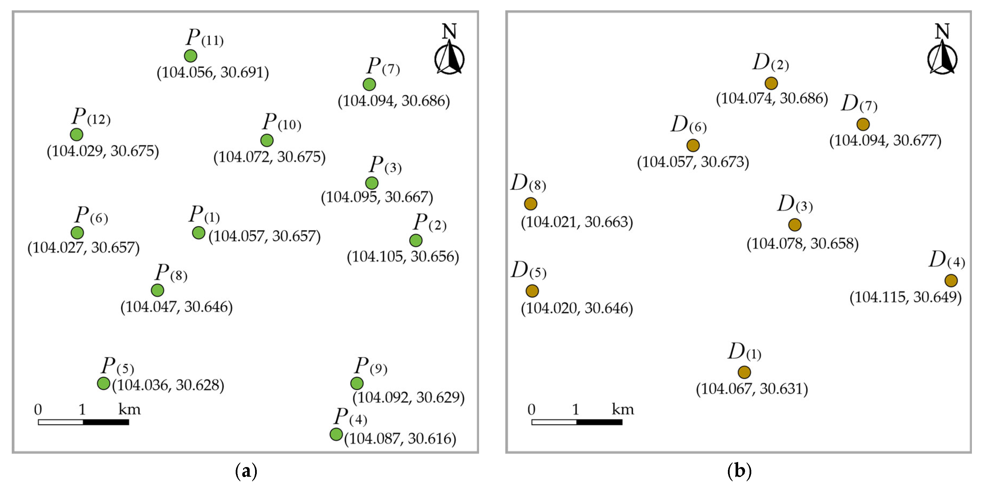
5. Conclusions

5.1. The Summary of the Research

Tourist cities based on the water ecological environment and water ecological POIs have the characteristics of a fragile water ecological environment, susceptibility to human activities, and difficulty in finding protection. Strengthening the protection of the water ecological environment and POIs is of great significance. We aim to optimize the material distribution of water ecological POIs and design methods to reduce the negative impact of the logistics systems on the water ecological POIs from the perspective of optimizing the material distribution routes and reducing pollutant emissions. We established the low-carbon water ecological POI logistics route-planning method based on the improved water network space AGNES clustering model and the symmetrical simulated Huffman spatial searching tree algorithm. The urban water network system is used as the basic structure for clustering the water ecological POIs and material distribution centers, and the improved AGNES algorithm is established for spatial clustering of water ecological POIs. As the starting and ending points of water ecological POI logistics routes, the optimal location of the distribution center is crucial. We constructed the logistics distribution center location model based on the water ecological POI clustering and selected the optimal distribution center from the perspective of the optimal closeness function. On the basis of determining the logistics route nodes, combining the symmetrical features of vehicles moving in the logistics sub-intervals and global logistics interval, the optimal path for each logistics sub-interval is determined by constructing the sub-interval optimal route-searching algorithm based on the symmetrical simulated Huffman spatial searching tree. Then, the global logistics route-planning algorithm based on the undirected complete graph spatial search is constructed to search for the global optimal logistics route. It can ensure that the logistics vehicle maintains symmetry in the moving distances on the round-trip vectors of the same distribution points and deliver orders under the same sub-interval path conditions. Experimental results show that our proposed algorithm can cluster the water ecological POIs reasonably, find out the optimal distribution center location, and output the logistics route with the lowest cost and minimal pollutant emissions. Compared with the traditional logistics route-planning algorithms, it has more advantages and can effectively reduce the negative impact of pollutants on the water ecological environment and water ecological POIs.

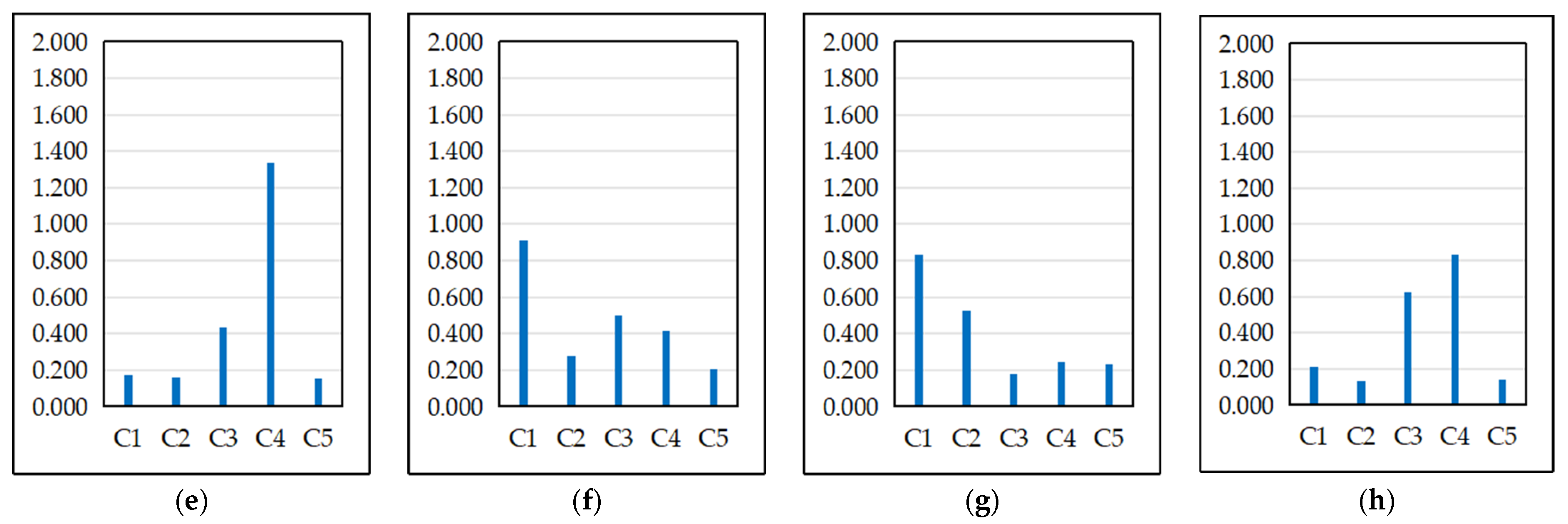
5.2. Innovation and Advantages of the Proposed Work

The constructed algorithm is an innovative method in the water ecological environment protection system, and its innovation and advantages are mainly reflected in the following aspects: firstly, research method innovation. The relevant literature has not constructed a method for the protection of the water ecological environment and water ecological POIs from the perspective of logistics system research. Our method constructs a model from the perspective of optimizing the logistics routes and reducing the pollutant emissions, with the goal of minimizing the logistics route costs and reducing the energy consumption and pollutant emissions during transportation, and thus reducing the damage to the water ecological POIs. The second aspect is that the designed model is innovative. In response to an urban spatial environment with abundant water ecological resources, we take into account the operating rules of logistics vehicles in the water network space when constructing the clustering algorithm. Based on the water network spatial structure, we establish the improved AGNES algorithm to establish the closeness relationship between the water ecological POIs, distribution centers, and water network spatial structure, which can effectively control the spatial scope of the logistics route planning and provide spatial conditions for optimizing logistics routes. At the same time, the constructed distribution center location model can find out the lowest cost distribution center, further controlling the cost of logistics routes. When constructing the logistics route algorithm, we model the spatial searching model on the selected distribution center and POIs to be delivered and output the logistics route with the optimal global cost to minimize the route cost. The third advantage is that the constructed algorithm has advantages over the traditional logistics route-planning algorithms. Analyzing the internal logic of algorithm design, the constructed algorithm adopts the idea of global optimization and can find out the global optimal route within logistics sub-intervals and logistics intervals. In the algorithm construction process, the designed improved AGNES clustering algorithm has lower time complexity and higher computational efficiency compared to the traditional algorithms of AGNES, k-means, and DBSCAN.

5.3. Limitation of the Proposed Work

Though the proposed algorithm has certain advantages compared to the traditional algorithms, there are still some limitations that need to be improved in future work. Firstly, the algorithm assumes that all POIs in the city have the same delivery priority, meaning that, in logistics algorithm logic, each POI has the feature of equality. In practical situations, seasonal variations in tourist numbers and relative differences in POI popularity can lead to differences in the demand for materials among different POIs, resulting in differences in delivery frequency, importance, priority, and other factors. Therefore, further consideration is needed on the role of POI priority in logistics algorithms. Secondly, the algorithm considers that all POIs have the same natural conditions, without considering the specific conditions of water ecological POIs (such as vulnerability of water ecological environment, size of water area, etc.), which may to some extent affect POI selection and logistics planning. Thirdly, the logistics distribution center location based on the frequency of POIs appearing in clusters is a local cost optimization method that can reduce logistics route costs to a certain extent. From the perspective of global POI distribution, the data accuracy for selecting distribution center location can be further improved. Fourthly, since the algorithm is modeled based on the given constraints and data foundation, without involving deep reinforcement learning and adaptive algorithms, it is suitable for logistics scenarios in which distribution points, distribution routes, time windows, distribution centers, and other conditions are predetermined. It is not suitable for scenarios in which logistics environments and conditions change dynamically at any time.

5.4. Future Work and Prospects

The constructed algorithm mainly targets the urban water ecological POIs and material distribution routes, and the research scope is the main urban area of water ecological tourism cities. In future research, we will conduct further research from the following aspects: firstly, we will deeply explore the tourism and spatial characteristics of the water ecological POIs, construct the spatial interest field strength of water ecological POIs from the perspective of tourism popularity, and use the POI spatial interest field strength as the screening condition for the urgency of material distribution, in order to determine the priority of POI distribution. Secondly, indicators such as water ecological vulnerability and water area size could be used to determine the priority of POI distribution, and these factors could be integrated into POI clustering and route planning to further optimize the algorithm and improve its application depth and breadth. Thirdly, the logistics distribution center location model could be further optimized by constructing a distribution center location model from the perspective of global spatial optimization, which links the distribution center location with global POIs, and could expand the scope of the distribution center location and the practicality of the proposed algorithm. Fourthly, it can be combined with deep reinforcement learning, adaptive algorithms, real-time traffic data, etc., to increase the learning performance of the algorithm and adapt to dynamic changes in logistics conditions [35]. With the development of the Internet of Things (IoT) and intelligent vehicle-networking technology, intelligent connected vehicles based on autonomous driving technology are the trend of future vehicle-networking development. Intelligent connected vehicles have functions such as automatic recognition, intelligent navigation, buffer searching, and intelligent data mining, which can be well integrated with the algorithms we have constructed. For example, using IoT sensors to detect POIs to be delivered within the buffer zone and using neural network algorithms to predict traffic congestion on logistics routes, etc. Therefore, in future work, further research could be conducted on the deep integration of intelligent connected vehicles and logistics planning, providing more decision support for smart logistics.

References

1. Pugliese, L.D.P.; Guerriero, F.; Miglionico, G. A revenue management approach for tourism logistics optimization. Int. Trans. Oper. Res. 2024, 32, 353–383. [Google Scholar] [CrossRef]
2. Dharmaratne, D.; Siriwardena, S.; Edirisinghe, L.; Silva, D.S. Interdependence of Logistics and Tourism: Crafting a Novel Logistics Concept in Tourism. Sustain. Dev. Res. 2023, 5, 87. [Google Scholar] [CrossRef]
3. Ruman, M.; Dąbrowska, D.; Rykała, W. Protection of Water Resources in Recreational Areas in Urban Space. Pol. Hyperb. Res. 2024, 86, 51–60. [Google Scholar] [CrossRef]
4. Zhou, J.L.; Yang, C.; Liu, D.D.; Wang, Y.Q.; Zhong, Z.M.; Wu, Y.N. A three-stage geospatial network optimal location decision model for urban green logistics centers from a sustainable perspective. Sustainable Cities and Society. Sustain. Cities Soc. 2025, 128, 106481. [Google Scholar] [CrossRef]
5. Onuigbo, A.C.; Onyia, C.O.; Onuigbo, O.T.; Nnoduo, C.C. Stream water protection strategies and prospects for bioresources protection and sustainable management. Int. J. Energy Water Resour. 2025, 9, 2809–2822. [Google Scholar] [CrossRef]
6. Gao, X.R.; Shao, S.; Gao, Q.F.; Zhang, Y.; Wang, X.M.; Wang, Y. Factors influencing carbon emissions and low-carbon paths in China’s transportation industry. Energy 2025, 323, 135778. [Google Scholar] [CrossRef]
7. Zhang, C.L.; Tang, L.Q.; Zhang, J.; Gou, L.M. Optimizing Distribution Routes for Chain Supermarket Considering Carbon Emission Cost. Mathematics 2023, 11, 2734. [Google Scholar] [CrossRef]
8. Da, Z.Y.; Yang, W.J.; Ran, P.P.; Qian, X.G.; Shao, S.; Pan, S.; Shi, B.J.; Li, Y.; He, R.L.; Xiao, Y.H. Design of Logistics Route Planning for Printing Enterprises Based on Baidu Map. ITM Web Conf. 2017, 11, 10001. [Google Scholar] [CrossRef]
9. Zhang, H. An optimisation method of factory terminal logistics distribution route based on K-means clustering. Int. J. Manuf. Technol. Manag. 2023, 37, 184–198. [Google Scholar] [CrossRef]
10. Puspitasari, F.H.; Kurniawan, V.R.B. Designing Optimal Distribution Routes using a Vehicle Routing Problem (VRP) Model in a Logistics Service Provider. IOP Conf. Ser. Mater. Sci. Eng. 2021, 1071, 012005. [Google Scholar] [CrossRef]
11. Febriandini, I.F.; Yuniaristanto, Y.; Sutopo, W. Multi-Compartment Vehicle Routing Problem to Find the Alternative Distribution Route of Petroleum Product Delivery. IOP Conf. Ser. Mater. Sci. Eng. 2020, 943, 012039. [Google Scholar] [CrossRef]
12. Kleinová, K.; Straka, M. Streamlining Distribution Routes Using the Language Model of Artificial Intelligence. Sustainability 2024, 16, 6890. [Google Scholar] [CrossRef]
13. Sembiring, C.A.; Sanjaya, A.; Willyanto, W. Optimal distribution route to minimize transportation costs in soft drink industry. J. Phys. Conf. Ser. 2019, 1402, 022048. [Google Scholar] [CrossRef]
14. Ma, C.L.; Yang, Y.Y.; Wang, L.H.; Chu, C.; Ma, C.; An, L.H. Research on distribution route with time window and on-board constraint based on tabu search algorithm. EURASIP J. Wirel. Commun. Netw. 2019, 2019, 25. [Google Scholar] [CrossRef]
15. Adam, N.A.F.P.; Sari, I.P.; Tasya, A.; Sutopo, W.; Yuniaristanto, Y. Determination of Routes for Daily Newspaper Product Distribution with Saving Matrix Methods. IOP Conf. Ser. Mater. Sci. Eng. 2020, 943, 012040. [Google Scholar] [CrossRef]
16. Wang, S.Y.; Sun, H. Distribution Route Planning for Cold Chain Items under Variable Demand. J. Highw. Transp. Res. Dev. 2015, 9, 103–110. [Google Scholar] [CrossRef]
17. Bukhari, H.; Basingab, M.S.; Rizwan, A.; Sánchez-Chero, M.; Pavlatos, C.; More, L.A.V.; Fotis, G. Sustainable green supply chain and logistics management using adaptive fuzzy-based particle swarm optimization. Sustain. Comput. Inform. Syst. 2025, 46, 101119. [Google Scholar] [CrossRef]
18. Gu, Y.J. Logistics route optimization based on improved shark optimization algorithm. Procedia Comput. Sci. 2025, 262, 1322–1328. [Google Scholar] [CrossRef]
19. Gan, Q. A logistics distribution route optimization model based on hybrid intelligent algorithm and its application. Ann. Oper. Res. 2022, 1–13. [Google Scholar] [CrossRef]
20. Liu, T.; Cheng, P. Research on Logistics Delivery Path Optimization Based on Deep Reinforcement Learning. J. Circuits Syst. Comput. 2025, 35, 2550360. [Google Scholar] [CrossRef]
21. Xu, Y.N.; Qin, J.X.; Zhou, Y.Q.; Wu, T. Analysis and Research of uncertain radius in constructing geo-spatial buffer. J. Phys. Conf. Ser. 2021, 1732, 012153. [Google Scholar] [CrossRef]
22. Yu, G.J. Analysis and Assessment of Geospatial Distribution of Tourism Resources in Ganzhou. Master’s Thesis, East China University of Technology, Fuzhou, China, June 2022. [Google Scholar]
23. Kushal, P.; Seema, N. A review of urban water networks management using GIS. MethodsX 2023, 11, 102261. [Google Scholar] [CrossRef] [PubMed]
24. Di Nardo, A.; Boccelli, D.L.; Herrera, M.; Creaco, E.; Cominola, A.; Sitzenfrei, R.; Taormina, R. Smart Urban Water Networks: Solutions, Trends and Challenges. Water 2021, 13, 501. [Google Scholar] [CrossRef]
25. Guo, R.Y.; Wang, Y.; Fan, J.X.; Fan, W.B. Embedding Hierarchical Cubic Networks into k-Rooted Complete Binary Trees for Minimum Wirelength. Int. J. Found. Comput. Sci. 2024, 35, 327–352. [Google Scholar] [CrossRef]
26. Wang, Y.Y. Research on Distributed Permutation Flow Shop Scheduling Based on AGNES Algorithm. Master’s Thesis, Tianjin University of Technology, Tianjin, China, January 2023. [Google Scholar]
27. Aliei, M.; Hoorali, M. Location of multi-product and multi-resource capacity facilities in green logistics. Int. J. Logist. Syst. Manag. 2025, 51, 133–149. [Google Scholar] [CrossRef]
28. Ma, H.X.; Zheng, X.Y.; Liang, H.J.; Luo, P. Logistics Center Selection and Logistics Network Construction from the Perspective of Urban Geographic Information Fusion. Sensors 2024, 24, 1878. [Google Scholar] [CrossRef]
29. Temjanovski, R.; Jovanov, T. Transforming freight mobility in the cities and promoting of green logistics. Maced. Int. J. Mark. 2020, 6, 113–121. [Google Scholar]
30. Giuffrida, N.; Calleo, Y.; Zio, S.D.; Pilla, F.; Ottomanelli, M. Spatial participatory planning for urban logistics: A GIS-enhanced Real-Time Spatial Delphi approach. Res. Transp. Econ. 2024, 108, 101488. [Google Scholar] [CrossRef]
31. Wang, L.L. A Model for Defining the Boundaries of Complex Sentences and Clauses in English Translation Based on the Huffman Tree and Objective Function. Int. J. High Speed Electron. Syst. 2025, 34, 2540117. [Google Scholar] [CrossRef]
32. Hiroshi, F.; Yuichi, S.; Hiroaki, Y. The Huffman Tree Problem with Upper-Bounded Linear Functions. IEICE Trans. Inf. Syst. 2022, E105.D, 474–480. [Google Scholar] [CrossRef]
33. Alsaleh, A. Electric and Autonomous Vehicles in Italian Urban Logistics: Sustainable Solutions for Last-Mile Delivery. World Electr. Veh. J. 2025, 16, 338. [Google Scholar] [CrossRef]
34. Santiago, L.R.M.; Lozano, A. Mathematical problems for designing a short-distance relief goods distribution network in urban areas. Transp. Res. Procedia 2024, 78, 281–288. [Google Scholar] [CrossRef]
35. Hazem, Z.B.; Saidi, F.; Guler, N.; Altaif, A.H. Reinforcement learning-based intelligent trajectory tracking for a 5-DOF Mitsubishi robotic arm: Comparative evaluation of DDPG, LC-DDPG, and TD3-ADX. Int. J. Intell. Robot. Appl. 2025, 1–21. [Google Scholar] [CrossRef]
Figure 1. The main content, structure, and logical relationships between the constructed algorithms of the work. (a) shows the main content and structure of the work, and (b) shows the logical relationships between the proposed improved AGNES clustering, the simulated Huffman spatial searching tree algorithm, and the logistics route algorithm.
Symmetry 17 01894 g001aSymmetry 17 01894 g001b
Figure 2. The generating process of the N E T R o , W M S , dataset W and elements W ( i ) , cluster C ( i ) buffer zones, and control point sets C o n ( i ) by the urban water network channels and main roads in the coordinate system x o y . (a) shows the constructed main water network meta-structure ( W M S ), (b) shows the constructed main road network ( N E T R o ), (c) shows the constructed river projection dataset W , (d) shows the constructed water network cluster C ( i ) and the buffer zone, (e) shows the overlay model of W M S and N E T R o , and (f) shows the constructed cluster control point set C o n ( i ) . In (a), the blue color curves represent the rivers. In (b), the brown color line represents the main road, blue and green color represents the water ecological POI. In (d,f), different colors for areas represent the buffer zones. In (e,f), the red nodes are the confluences of roads and river W ( 5 ) ; The light green nodes are the confluences of roads and river W ( 4 ) ; The dark blue nodes are the confluences of roads and river W ( 3 ) ; The dark green nodes are the confluences of roads and river W ( 2 ) ; The orange nodes are the confluences of roads and river W ( 1 ) ; The light blue nodes are the confluences of roads and river W ( 6 ) .
Symmetry 17 01894 g002aSymmetry 17 01894 g002b
Figure 3. The process of constructing the complete binary tree T W ( i ) based on the river channel elements W ( i ) and control point sets C o n ( i ) . (a) shows the cluster control point sets C o n ( i ) , (b) shows the selected sample cluster control point set C o n ( 1 ) , (c) shows the water ecological POI clustering objective function model f [ P ( i ) , C o n ( i , j ) ] , and (d) shows the generated water ecological POI clustering complete binary tree T W ( i ) based on C o n ( 1 ) .
Symmetry 17 01894 g003aSymmetry 17 01894 g003b
Figure 4. The process of constructing the clustering algorithm model.
Symmetry 17 01894 g004
Figure 5. The process of constructing the distribution center location algorithm model.
Symmetry 17 01894 g005
Figure 6. The process of constructing the sub-interval coordinate system x o , the sub-intervals ζ [ K ( i ) , K ( i + 1 ) ] ( t ) , and the directed weighted edge graph G ( i ) between the urban water ecological POIs by the N E T R o . (a) shows the road network, road nodes, and the constructed N E T R o within the buffer zone of POIs; (b) shows the constructed coordinate system x o y for N E T R o based on (a); (c) shows the process of selecting the key control points C ( i ) from the coordinate system x o y , determining K ( i ) and K ( i + 1 ) to form the sub-interval ζ [ K ( i ) , K ( i + 1 ) ] ( t ) ; (d) shows the directed weighted edge graph G ( i ) = < V , E > and sub-interval ζ [ K ( i ) , K ( i + 1 ) ] ( t ) .
Symmetry 17 01894 g006
Figure 7. The constructed symmetrical simulated Huffman spatial searching tree model SHSST. The route formed by the red color arrows represents the optimal route.
Symmetry 17 01894 g007
Figure 8. The constructed undirected complete graph G ( i ) * of the logistics route interval and the example of the correlation vectors of each vertex obtained after the discretization of graph G ( i ) * . (a) shows the undirected complete graph G ( i ) * , and (b) is the example of the correlation vectors of each vertex obtained after the discretization of graph G ( i ) * .
Symmetry 17 01894 g008
Figure 9. The modeling process of the global logistics route-planning algorithm based on undirected complete graph spatial search.
Symmetry 17 01894 g009
Figure 10. The collected data of N E T R o and W M S in the experiment. (a) shows the water spatial scope of Chengdu city, in which all the Chinese names of map annotations come from Chinese Baidu Map; (b) shows the main road data as the structure of N E T R o ; In (c), we use the confluence points of the four rivers as boundaries to divide the rivers into different sections and establish W M S and the river projection dataset W ; (d) shows the initial buffer zone of the water ecological POI cluster C ( i ) ; (e) includes each element W ( i ) and the generated control points C o n ( i , j ) , in which the number represents the control point sequence. (f) shows the cluster control point set C o n ( i ) , in which the number represents the control point sequence.
Symmetry 17 01894 g010aSymmetry 17 01894 g010b
Figure 11. The spatial relationship between the collected water ecological POIs, distribution centers, and control points in the urban coordinate system. (a) shows the location projection of water ecological POIs; (b) shows the location projection of distribution centers; (c) shows the location of water ecological POIs, distribution centers, W M S , and control points C o n ( i , j ) in the urban geographic space, in which the number represents the control point sequence; (d) shows the spatial relationship structure of the projections on water ecological POIs, distribution centers, W M S , and control point C o n ( i , j ) , in which the number represents the control point sequence.
Symmetry 17 01894 g011aSymmetry 17 01894 g011b
Figure 12. The comparison of the optimal objective functions for the control point sets C o n ( i ) and clusters C ( i ) corresponding to POIs. The (al) relate to the POIs P ( 1 ) ~ P ( 12 ) .
Symmetry 17 01894 g012aSymmetry 17 01894 g012b
Figure 13. The comparison of the optimal objective functions for each cluster control point set C o n ( i ) and cluster C ( i ) corresponding to the distribution center D ( i ) . The (ah) relate to the distribution centers D ( 1 ) ~ D ( 8 ) .
Symmetry 17 01894 g013aSymmetry 17 01894 g013b
Figure 14. The complete binary tree T f ( u ) corresponding to the global logistics routes and cost function values f [ D ( i ) , D ( i ) ] ( u ) output by the algorithm.
Symmetry 17 01894 g014
Figure 15. The change curves of cost function values for each logistics sub-interval output by the experimental group and the control group. (a) is the sub-interval cost function value curve of the experimental group PSA, (b) is the sub-interval cost function value curve of the control group IDA, and (c) is the sub-interval cost function value curve of the control group IPA.
Symmetry 17 01894 g015
Figure 16. The cost error values of the experimental group and the control group in each sub-interval. (a) represents the sub-interval error of PSA relative to IDA, and (b) represents the sub-interval error of PSA relative to IPA.
Symmetry 17 01894 g016
Figure 17. Complete binary trees of global logistics cost output by the experimental group and the control group. (a) shows the output of the complete binary tree by the experimental group PSA; (b) shows the output of the complete binary tree by the control group IDA; (c) shows the output of the complete binary tree by the control group IPA.
Symmetry 17 01894 g017
Figure 18. The comparison of the optimal route output by the experimental group and the control group in terms of cost function value, route cost, and optimization rate. (a) shows the optimal route cost function values output by the experimental group and the control group; (b) shows the optimal route cost output by the experimental group and the control group; (c) shows the errors of the optimal route cost function values output by the experimental group and the control group; (d) shows the errors of the optimal route cost output by the experimental group and the control group; (e) shows the comparison of the optimal route cost optimization rate output by the experimental group and the control group.
Symmetry 17 01894 g018
Figure 19. The total pollutant emissions m of the experimental group and the control group, as well as the total reduction Δ m in pollutant emissions of the experimental group compared to the control group. (a) shows the total pollutant emissions m of the experimental group and the control group, with blue representing PSA, orange representing IDA, and green representing IPA. (b) shows the total reduction Δ m in pollutant emissions between the experimental group and the control group, blue represents the difference between PSA and IDA, while orange represents the difference between PSA and IPA.
Symmetry 17 01894 g019
Figure 20. Comparison of the optimization rate of random logistics routes between experimental group and control group. (a) represents Group 1, and (b) represents Group 2, in which the blue bar represents the optimization rate (difference) of PSA relative to IDA, and the orange bar represents the optimization rate (difference) of PSA relative to IPA.
Symmetry 17 01894 g020