Incorporating Parameter Uncertainty into Copula Models: A Fuzzy Approach

Abstract

This paper proposes a fuzzy copula-based optimization framework for modeling dependence structures and financial risk under parameter uncertainty. The parameters of selected copula families are represented as trapezoidal fuzzy numbers, and their α-cut intervals capture both the support and core ranges of plausible dependence values. This fuzzification transforms the estimation of copula parameters into a fuzzy optimization problem, enhancing robustness against sampling variability. The methodology is empirically applied to gold and oil futures (1 January 2015–1 January 2025), comparing symmetric copulas, i.e., Gaussian and Frank and asymmetric copulas, i.e., Clayton, Gumbel and Student-t. The results prove that the fuzzy copula framework provides richer insights than classical point estimation by explicitly expressing uncertainty in dependence measures (Kendall’s τ, Spearman’s ρ) and risk indicators (Value-at-Risk, Conditional Value-at-Risk). Rolling-window analyses reveal that fuzzy VaR and fuzzy CVaR effectively capture temporal dependence shifts and tail severity, with fuzzy CVaR consistently producing more conservative risk estimates. This study highlights the potential of fuzzy optimization and fuzzy dependence modeling as powerful tools for quantifying uncertainty and managing extreme co-movements in financial markets.

1. Introduction

The interdependence between financial assets plays a critical role in portfolio diversification, hedging, and systemic risk assessment. However, conventional statistical approaches often assume precise parameter estimates and stable dependence structures, which may not hold in real-world markets characterized by uncertainty, volatility, and incomplete information. In such contexts, reflecting both the symmetry and asymmetry of dependence as well as the uncertainty in model parameters becomes essential for accurate risk evaluation.

Copula models have emerged as a powerful framework for analyzing nonlinear and non-Gaussian dependencies between financial variables, allowing for the separation of marginal behavior from joint dependence (Embrechts et al., 2002 [1]). Parameter estimation in copulas is inherently sensitive to sampling variability and model specification errors. This uncertainty can significantly affect dependence measures such as Kendall’s τ and Spearman’s ρ, and consequently distort risk indicators like Value-at-Risk (VaR) and Conditional Value-at-Risk (CVaR) (Artzner et al., 1999 [2]; Just & Łuczak, 2020 [3]). To deal with this issue, recent studies (Just & Luczak, 2020 [3]; Zhou et al., 2023 [4]) have sought to integrate fuzzy set theory into dependence modeling, introducing fuzziness into copula parameters to better represent epistemic uncertainty.

Building on these developments, this paper proposes a fuzzy copula-based optimization framework that models dependence structures and financial risk under parameter uncertainty.

The methodology uses trapezoidal fuzzy numbers to represent uncertain copula parameters and α-cut decomposition to evaluate corresponding intervals of dependence and risk (Buckley, 2005 [5]). This fuzzification transforms the estimation problem into a fuzzy optimization one, providing a more robust characterization of dependence than traditional point estimation.

The empirical analysis focuses on the gold (GC = F) and crude oil (CL = F) futures markets over the period 1 January 2015–1 January 2025, using daily data obtained from Yahoo Finance. These commodities are chosen due to their central role in global financial and energy systems, as well as their complex interdependence patterns that fluctuate across market regimes. By comparing symmetric (Gaussian, Frank) and asymmetric (Clayton, Gumbel, Student-t) copulas, the study explores how fuzziness affects dependence estimation and risk evaluation across different tail behaviors.

Beyond the theoretical construction of fuzzy copulas, this study extends the analysis through a sequence of complementary empirical procedures designed to uncover the temporal dynamics and structural characteristics of risk. First, the paper computes fuzzy dependence measures—Kendall’s τ and Spearman’s ρ—across multiple copula families and α-cuts, providing an interval-based perspective on the strength and uncertainty of interdependence.

Second, fuzzy risk indicators are derived through the VaR and CVaR measures. By simulating returns from copulas with fuzzy parameters, these indicators become fuzzy numbers themselves, expressing uncertainty about potential portfolio losses. Fuzzy VaR captures the quantile of extreme loss distributions, while fuzzy CVaR extends the analysis by assessing expected shortfalls beyond the VaR threshold, offering a deeper and more conservative view of tail risk.

Finally, a rolling-window procedure is implemented to evaluate the time-varying nature of fuzzy risk and dependence. This dynamic framework enables the identification of structural breaks and crisis periods—particularly around 2020–2021—where tail co-movements intensify. Rolling fuzzy VaR and CVaR reveal not only how downside risk evolves over time but also how the shape and magnitude of uncertainty change with market regimes.

The main contributions of this study can be summarized as follows:

• We develop a fuzzy copula-based optimization framework that integrates parameter uncertainty into dependence modeling, transforming point estimation into a fuzzy optimization problem.
• We introduce the use of trapezoidal fuzzy numbers and the α-cut to introduce the epistemic uncertainty in copula parameters, resulting in interval-based measures of dependence and risk.
• We propose an empirical validation to gold and oil futures (1 January 2015–1 January 2025), comparing symmetric and asymmetric copulas with fuzzified parameters to capture uncertainty in tail dependence.
• We compute fuzzy versions of VaR and CVaR to account for parameter uncertainty and asymmetric tail behavior.
• We apply a rolling window analysis to assess the dynamic behavior of fuzzy dependence and risk, to better understand temporal evolution of tail risk.

The paper is organized as follows. Section 2 reviews the main theoretical and empirical contributions to copula modeling and symmetry analysis in dependence structures. Section 3 introduces the fuzzy optimization and copula methodology, outlining the construction of trapezoidal fuzzy parameters and the α-cut procedure. Section 4 presents the empirical results on fuzzy dependence measures, followed by Section 5, which details the case study on the Gold–Oil portfolio, including fuzzy VaR and CVaR estimations. Section 6 extends the analysis using rolling windows to assess the time-varying behavior of fuzzy risk measures and decision dynamics. Section 7 concludes with the main findings, discusses methodological limitations, and suggests directions for future research.

2. Literature Review

Copula models have become necessary tools in capturing nonlinear and asymmetric dependence structure between financial variables. Building on Sklar’s theorem (Sklar, 1959 [6]), copulas allow the separation of marginal distributions from joint dependence structure, having greater flexibility in modeling risk and co-movement. In the past two decades, several studies have applied copulas to financial markets to reflect dependence dynamics in both normal and turbulent periods. Ismail et al. (2023) [7] provided a comprehensive review of copula theory and its evolution. They emphasized how dependence modeling has advanced from simple elliptical copulas to dynamic and high-dimensional structures.

For high-dimensional dependence structures, vine copulas (pair-copula constructions) have become the state-of-the-art due to their flexibility and tractability beyond traditional elliptical and Archimedean families (Czado & Nagler, 2022 [8]; Cheng et al., 2025 [9]).

In empirical finance, copula-based models have been used to uncover nonlinear and asymmetric relationships between asset classes. Dewick and Liu (2022) [10] combined ARMA–GARCH models to analyze the dependence between crude oil and natural gas returns, finding limited co-movement across regimes. Chang (2021) [11] proposed a dynamic mixture copula model with time-varying parameters, capturing changing tail dependencies among stock-exchange rate pairs. Saekow et al. (2025) [12] proposed a mixture of Survival Clayton and Survival Gumbel copulas to model contagion between global and national stock markets. They show that tail dependence intensifies during crisis periods such as COVID-19. Deng et al. (2025) [13], who employed large skew-t copula models, confirm that asymmetric structures better explain financial contagion and co-movements than symmetric ones. Mukherjee et al. (2018) [14] developed a new class of bivariate asymmetric copulas based on products of symmetric (and sometimes asymmetric) copulas with powered arguments. Their approach, validated on real datasets such as car rental and economic indicators, proved superior goodness-of-fit compared to existing copulas.

A parallel strand of research has focused on symmetry properties within dependence structure. Jaser and Min (2021) [15] introduced simple nonparametric tests to detect symmetry and radial symmetry in bivariate copula data and to assess whether a dependence structure can be represented by an elliptical copula. Billio et al. (2022) [16] proposed a fast test for copula radial symmetry using a multiplier bootstrap approach and an equivalent randomization approach. Simulations confirmed the superior performance of the randomization method, and its application to EU industrial production indices revealed significant radial asymmetry. Jiménez-Varón et al. (2025) [17] introduced functional boxplot visualization and rank-based testing for copula symmetry, offering a powerful graphical approach to detect departures from reflection and joint symmetry in financial time series.

Another emerging direction involves the inclusion of uncertainty and fuzziness into dependence modeling. Copula estimation relies on point parameters, which may inadequately represent epistemic uncertainty, especially in small samples or volatile markets. Just and Łuczak (2020) [3] integrated fuzzy clustering into copula-GARCH models to account for imprecise dependence. Zhou et al. (2023) [4] proposed interval-based dependence measures using fuzzy sets, emphasizing the propagation of epistemic uncertainty in copula parameters. Zachariah et al. (2025) [18] extended copula-based information theory by introducing a cumulative copula Tsallis entropy framework, which quantifies dependence and uncertainty more flexibly than Shannon entropy. Romagnoli (2020) [19] contrasts conditional versus unconditional fuzzy–copula formulations. Araichi and Almuhim (2021) [20] or Bernardi et al. (2023) [21] embed fuzzy inference and fuzzy measure changes into vine and Esscher–copula frameworks. Yu et al. (2025) [22] use a fuzzy–copula GMM with Kullback–Leibler divergence for commodity hedging. Li et al. (2023) [23] integrate copulas, fuzzy–rough sets and Bayesian networks for dependence modelling under subjective uncertainty.

Compared with the existing body of work, this study differs both in scope and methodology. Previous studies often focus on specific aspects of dependence modeling: parameter fuzzification, entropy-based analysis, or sector-specific risk estimation. Our approach simultaneously incorporates epistemic uncertainty, tail asymmetry, and temporal dynamics. By combining fuzzy set theory with copula symmetry analysis and dynamic rolling-window estimation, the present framework provides a coherent method for analyzing complex and evolving dependence patterns.

3. Methodology

Fuzzy set theory, introduced by Zadeh (1965) [24], provides a mathematical framework for handling vagueness and imprecision in decision-making. A fuzzy set $\tilde{A}$ in a universe of discourse X is defined by its membership function ${\mu }_{\tilde{A}}:X\to [0, 1]$, $\tilde{A}=\left\{\right(x,{\mu }_{\tilde{A}}\left(x\right)\left)\right|x\in X\}$. When optimization problems involve imprecise coefficients or constraints, the use of fuzzy numbers allows incorporating uncertainty into the model (Dubois & Prade, 1980 [25]).

A trapezoidal fuzzy number $\tilde{\theta }=(a_1,a_2,a_3,a_4)$ is commonly used, with membership function:

$${\mu }_{\tilde{\theta }}\left(x\right)=\left\{\begin{array}{c}0,x\le a_1,\\ {\displaystyle \frac{x-a_1}{a_2-a_1}},a_1\le x\le a_2,\\ 1,a_2\le x\le a_3,\\ {\displaystyle \frac{a_4-x}{a_4-a_3}},a_3\le x\le a_4,\\ 0,x\ge a_4\end{array}\right.$$

(1)

This representation is particularly useful in optimization since the core $[a_2,a_3]$ and the support $[a_1,a_4]$ reflect confidence intervals around estimated parameters (Buckley, 2005 [5]).

Optimization problems often exhibit symmetry between maximization and minimization (duality). In fuzzy programming, this symmetry can be expressed by considering the α-cuts of fuzzy numbers (Dubois & Prade, 1980 [25]):

$${[\tilde{\theta }]}_{\alpha }=\{x\in \mathbb{K}{\mu }_{\tilde{\theta }}\left(x\right)\ge \alpha \}=[{\theta }_{\alpha }^{-},{\theta }_{\alpha }^{+}]$$

(2)

which reduces a fuzzy optimization problem to a family of crisp optimization problems parameterized by $\alpha \in [0,1]$. The α-cut of a trapezoidal fuzzy number $\tilde{\theta }$ has the form (Dubois and Prade, 1980 [25], Georgescu, 2012 [26]):

$${[\tilde{\theta }]}_{\alpha }=\left[a_1+\alpha \left(a_2-a_1\right),a_4-\alpha \left(a_4-a_3\right)\right], \alpha \in [0,1]$$

(3)

Thus, the duality principle in fuzzy optimization is realized through the symmetric evaluation of lower and upper bounds across α-cuts, linking the concept of supremum/infimum in fuzzy set theory with classical optimization (Bellman & Zadeh, 1970 [27]).

In dependence modeling, copulas provide a flexible tool for linking joint and marginal distributions. First, we give the following definition of a copula (Kwofie et al., 2020 [28]):

Definition 1. 

A two-dimensional copula function $C:{[0, 1]}^2\to [0, 1]$ satisfies:

(1)

$C\left(u,0\right)=C\left(0,v\right)=0,\forall u,v\in [0,1]$

(2)

$C\left(u,1\right)=u$ and $C\left(1,v\right)=v$, $\forall u,v\in [0,1]$

(3)

$C\left(u_2,v_2\right)-C\left(u_2,v_1\right)-C\left(u_1,v_2\right)+C(u_1,v_1)\ge 0$, $\forall u,v\in [0,1]$.

According to Sklar’s theorem (1959) [6], for any bivariate distribution function H(x, y) with continuous margins $F_X\left(x\right)$ and $F_Y\left(y\right)$, there exists a copula C such that:

$$H\left(x,y\right)=C(F_X\left(x\right),F_Y\left(y\right);\theta )$$

(4)

θ is the copula parameter (or set of parameters) that governs how strongly (and in which tail) the variables are dependent, beyond their marginal distributions.

Different families of copulas capture different patterns of dependence. The Clayton copula (Clayton, 1978) [29] emphasizes lower-tail dependence and is defined by:

$$C_{\theta }\left(u,v\right)={(\mathrm{m}\mathrm{a}\mathrm{x}\{u^{-\theta }+v^{-\theta }-1, 0\})}^{-1/\theta }, \theta >0,$$

(5)

The Gumbel copula (Gumbel, 1960) [30] captures upper-tail dependence:

$$C_{\theta }\left(u,v\right)=\mathrm{e}\mathrm{x}\mathrm{p}(-{[{(-\ln u)}^{\theta }+{(-\ln v)}^{\theta }]}^{1/\theta }), \theta \ge 1$$

(6)

The Frank copula (Frank, 1979) [31] models symmetric dependence with no tail preference:

$$C_{\theta }\left(u,v\right)=-{\displaystyle \frac{1}{\theta }}\mathrm{l}\mathrm{n}(1+{\displaystyle \frac{(e^{-\theta u}-1)(e^{-\theta v}-1)}{e^{-\theta }-1}}), \theta \ne 0$$

(7)

The Gaussian copula (Embrechts et al., 2002) [1] is based on the correlation structure of the multivariate normal distribution:

$$C_{\rho }\left(u,v\right)={\Phi }_{\rho }({\Phi }^{-1}\left(u\right),{\Phi }^{-1}\left(v\right)), \rho \in [-\mathrm{1,1}]$$

(8)

$\Phi$ is the cumulative distribution function (CDF) of the univariate standard normal distribution, ${\Phi }^{-1}$ is the inverse CDF, ${\Phi }_{\rho }$ is the CDF of the bivariate normal distribution with correlation parameter $\rho$.

The Student-t copula introduced by Demarta and McNeil (2005) [32] extends the Gaussian copula with heavy tails:

$$C_{\rho ,\nu }\left(u,v\right)=t_{\rho ,\nu }(t_{\nu }^{-1}\left(u\right),t_{\nu }^{-1}\left(v\right))$$

(9)

where $t_{\nu }^{-1}$ is the quantile function of the univariate Student-t distribution and $t_{\rho ,\nu }$ is the bivariate Student-t distribution with correlation $\rho$ and degrees of freedom ν. The parameter ν governs the heaviness of the tails and the existence of statistical moments. For values of ν ≤ 1, even the mean of the distribution is undefined, which renders the copula unsuitable for dependence modeling. When 1 < ν ≤ 2, the mean exists, but the variance is infinite, preventing the definition of a valid correlation structure. To ensure both a finite mean and variance, and consequently a meaningful dependence parameter, the degrees of freedom are therefore restricted to ν > 2. Finite variance actually requires ν > 2; at ν = 2, the variance becomes infinite, while the mean exists only for ν > 1. Condition ν > 2 was strictly enforced in all computational procedures. Lower values of ν within this admissible range correspond to stronger tail dependence and heavier tails, making the Student-t copula particularly useful for extreme risk modeling, while higher values of ν lead the copula to converge toward the Gaussian case.

In practice, copula parameters such as θ or $\rho$ are estimated using maximum likelihood. To incorporate epistemic uncertainty, these estimates are fuzzified. If $\widehat{\theta }$ denotes the point estimate, the corresponding trapezoidal fuzzy number is constructed as:

$$\begin{gathered} \tilde{\theta }=(\hat{\theta }\left(1-{\delta }_1\right),\hat{\theta }\left(1-{\delta }_2\right),\hat{\theta }\left(1+{\delta }_2\right),\hat{\theta }\left(1+{\delta }_1\right)), \\ \mathrm{with} 0<{\delta }_2<{\delta }_{1.} \end{gathered}$$

(10)

The parameters ${\delta }_1$ and ${\delta }_2$ determine the width of the support and core intervals. For elliptical copulas, fuzzification is adjusted to maintain valid ranges, such as constraining ρ within [−1, 1].

Risk measures such as VaR and CVaR are widely used in finance (Artzner et al., 1999 [2]). For a portfolio return R, at confidence level p:

$${VaR}_p\left(R\right)=\mathrm{i}\mathrm{n}\mathrm{f}\{r\in \mathbb{R}:P(R\le r)\ge 1-p\}$$

(11)

$${CVaR}_p\left(R\right)=\mathbb{E}\left\{R\right|R\le {VaR}_p\left(R\right)\}$$

(12)

By simulating from copulas with fuzzy parameters $\tilde{\theta }$, the resulting VaR and CVaR become fuzzy numbers themselves. For each α-cut of the fuzzy parameter $\tilde{\theta }$, the parameter space is reduced to an interval. The VaR and CVaR are then computed for all values within this interval, yielding a corresponding range of risk measures.

$${\widetilde{VaR}}_p=\bigcup _{\alpha \in [0,1]}[{VaR}_p^{min}\left(\alpha \right),{VaR}_p^{max}\left(\alpha \right)]$$

(13)

$${\widetilde{CVaR}}_p=\bigcup _{\alpha \in [0,1]}[C{VaR}_p^{min}\left(\alpha \right),{CVaR}_p^{max}\left(\alpha \right)]$$

(14)

The notations ${VaR}_p^{min}\left(\alpha \right)$ and ${VaR}_p^{max}\left(\alpha \right)$ denote, respectively, the smallest and largest VaR values obtained at confidence level p when the copula parameters vary within the α-cut. Similarly, $C{VaR}_p^{min}\left(\alpha \right)$ and ${CVaR}_p^{max}\left(\alpha \right)$ represent the lower and upper bounds of the CVaR. These intervals reflect the uncertainty stemming from the fuzziness of the input parameters.

From a decision-making perspective, these fuzzy risk measures provide valuable flexibility. Conservative investors may focus on the upper bounds ${VaR}_p^{max}\left(\alpha \right)$ or, ${CVaR}_p^{max}\left(\alpha \right)$ which capture worst-case scenarios under both randomness and fuzziness. Conversely, more optimistic or risk-tolerant investors may rely on the lower bounds, ${VaR}_p^{min}\left(\alpha \right)$ or $C{VaR}_p^{min}\left(\alpha \right)$ which correspond to best-case estimates. The fuzzy interval as a whole provides a richer description of uncertainty than a single crisp value, allowing decision-makers to explicitly incorporate imprecision into their risk management strategies (Huang, 2007 [33]).

To ensure that the fuzzy bounds of ${\widetilde{VaR}}_p$ and ${\widetilde{CVaR}}_p$ fully capture the range of possible outcomes, we verified the monotonicity of VaR and CVaR with respect to the copula parameters within each α-cut interval. While most copula families (Clayton, Gumbel, Frank, and Gaussian) exhibit monotonic relationships between the dependence parameter and risk measures, the Student-t copula may display mild non-monotonic behavior due to its joint sensitivity to correlation and degrees of freedom. Therefore, for the Student-t case, a seven-point interior grid over each α-cut interval $\left[{\nu }_L\left(\alpha \right),{\nu }_U\left(\alpha \right)\right]$ was evaluated. The fuzzy lower and upper bounds correspond to the minimum and maximum VaR/CVaR values obtained over this grid, ensuring that no intermediate extreme was missed and that the fuzzy envelopes represent complete α-cut coverage.

Table 1. Characteristics of selected copula families used in dependence modeling.

Copula	Key Reference	Tail Dependence	Parameter Domain	Application Strength
Clayton	Clayton (1978) [29]	Lower tail	$\theta >0$	Crashes, downside risk
Gumbel	Gumbel (1960) [30]	Upper tail	$\theta \ge 1$	Booms, extreme highs
Frank	Frank (1979) [31]	None (symmetric)	$\theta \ne 0$	Moderate dependence
Gaussian	Embrechts et al. (2002) [1]	None	$\rho \in [-1, 1]$	Linear dependence
t-Copula	Demarta & McNeil (2005) [32]	Both tails	$\rho \in \left[-1,1\right], \nu \ge 2$	Extreme risk modeling

summarizes the main references, tail dependence properties, parameter domains, and application strengths of the five copula families (Clayton, Gumbel, Frank, Gaussian, and Student-t) employed in this study.

We use daily (trading-day frequency futures data for Gold (GC = F) and Crude Oil (CL = F) obtained from Yahoo Finance, covering the period 1 January 2015 to 1 January 2025, with the data pulled in October 2025. These series represent front-month continuous futures contracts, expressed in U.S. dollars, and were converted into logarithmic returns for subsequent empirical analysis. The daily front-month continuous futures for Gold (GC = F) and Crude Oil (CL = F) were retrieved from Yahoo Finance using the quantmod R package. (R Studio 2023.12.1) Each series represents the front-month continuous contract, which rolls automatically to the next active contract based on maximum trading volume (volume-based rule).

This roll mechanism ensures that, as the front-month contract approaches expiration, the data seamlessly transition to the next liquid contract, minimizing discontinuities. Yahoo Finance applies a backward adjustment to preserve price continuity across roll dates, preventing artificial jumps that might otherwise distort return calculations.

Consequently, all returns, dependence measures, and risk indicators in this study are computed using these volume-rolled, back-adjusted continuous futures. No additional manual roll adjustments were introduced.

The Gold–Oil portfolio is constructed using equal weights (0.5–0.5) for Gold and Oil, and the composition remains fixed throughout the sample period. No rebalancing is performed as the rolling window advances, ensuring that changes in fuzzy VaR and CVaR reflect evolving dependence and tail risk rather than portfolio adjustment.

The empirical part of the study was conducted in R, using packages such as copula for dependence modeling and FuzzyNumbers for the representation of fuzzy parameters. First, log-returns of financial assets were computed and transformed into uniform margins by empirical ranks. Next, copulas were fitted by maximum likelihood, and the estimated parameters were fuzzified into trapezoidal fuzzy numbers.

For each α–cut, we computed Kendall’s tau and Spearman’s rho by evaluating both lower and upper copulas. Kendall’s tau for a copula C is defined as:

$$\tau =4{\int }_0^1{\int }_0^{1}C\left(u,v\right)dC\left(u,v\right)-1$$

(15)

Meanwhile, Spearman’s rho is:

$$\rho =12{\int }_0^1{\int }_0^1\left(C\left(u,v\right)-uv\right)dudv$$

(16)

The constants 4 and 12 serve as normalization factors, ensuring that both measures lie in [−1, 1] and yield 0 for independence.

For Archimedean copulas (Clayton, Gumbel, Frank), closed forms exist for both τ and ρ. For the Gaussian copula, these measures are derived directly from the correlation parameter. For the Student-t copula, however, Spearman’s rho lacks a closed form and was approximated by Monte Carlo simulation from copula samples.

In R, we implemented this through the functions fuzzy_tau() and fuzzy_rho(), looping across α–cuts and computing dependence intervals.

The trapezoidal fuzzy parameters were defined around the maximum likelihood estimate (MLE) $\widehat{\theta }$ of the copula parameters. To capture uncertainty, perturbations of ±10% and ±20% were applied. The core interval $[a_2,a_3]$ was specified as ±10% around the MLE, representing the range within which the true parameter is most confidently expected to lie. The support interval $[a_1,a_4]$ extended to ±20% around the MLE, reflecting the full plausible uncertainty range.

This is a common heuristic in financial risk modeling, while alternative approaches such as confidence interval–based fuzzification (see Zhou et al., 2023 [4]) could also be employed to ensure robustness.

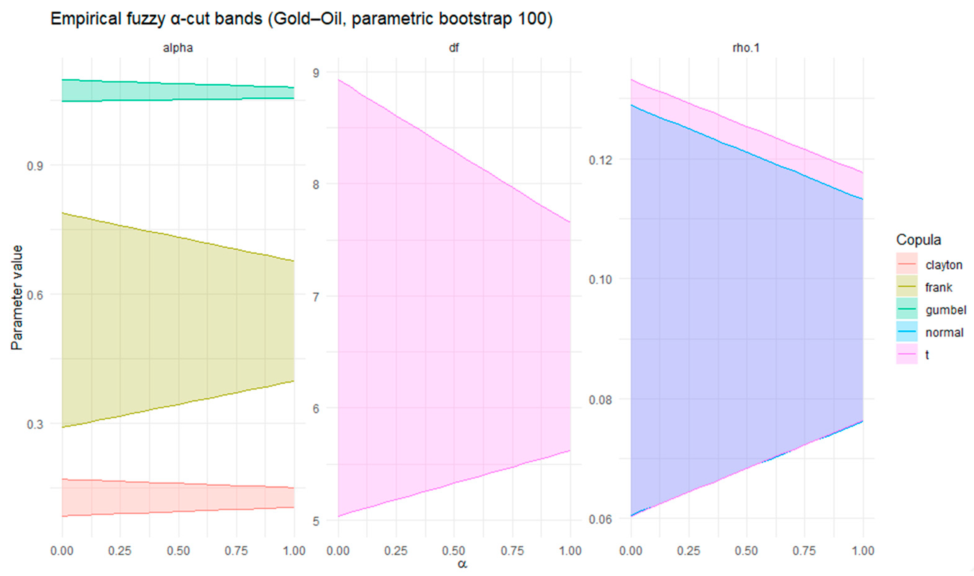
To empirically ground the ±10/±20% heuristic used for defining fuzzy cores and supports, we additionally derived fuzzy α-cut intervals from parametric bootstrap replications of the copula models in Appendix B.

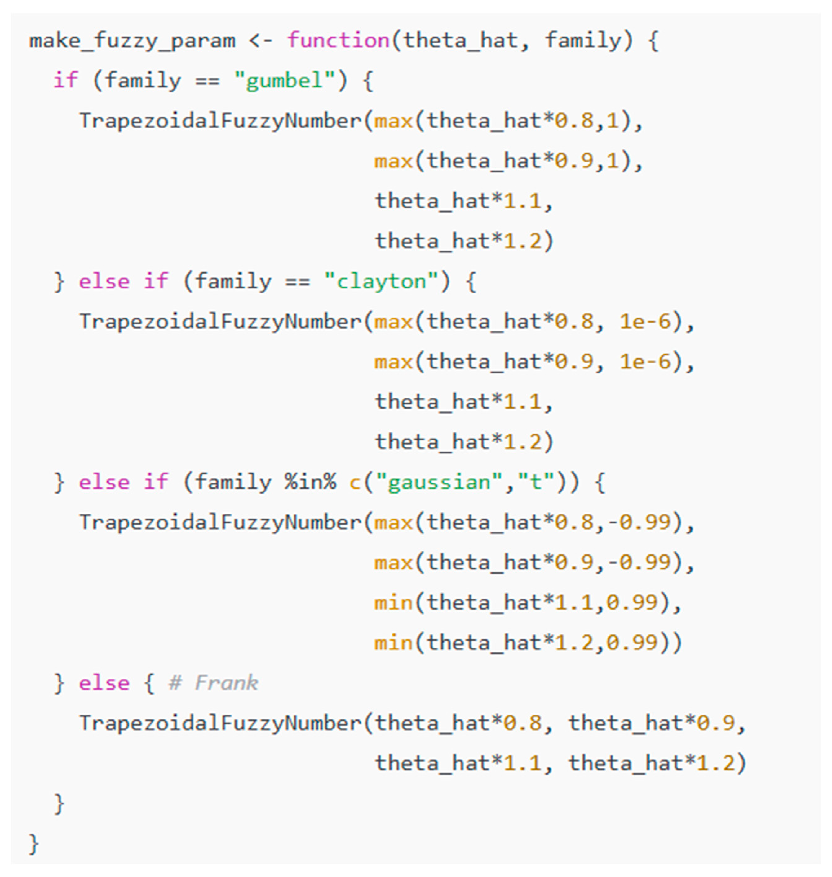
Because copula families impose restrictions on their parameters, the fuzzy numbers were adapted as follows. For the Clayton copula ($\theta >0$), the lower bounds were truncated to ensure positivity, using, i.e., $\mathrm{m}\mathrm{a}\mathrm{x}(0.8\widehat{\theta },{10}^{-6})$. For the Gumbel copula ($\theta \ge 1$), the lower support and core were restricted to be at least 1, i.e., $\mathrm{m}\mathrm{a}\mathrm{x}(0.8\widehat{\theta },1)$. The Frank copula $\theta \in \mathbb{R}\setminus \left\{0\right\}$ is unconstrained, and thus symmetric perturbations around the point estimate were applied. For the Gaussian copula ($\rho \in (-1, 1)$) the fuzzy number was bounded within the admissible range, truncated to [−0.99,0.99] to avoid singularities. Finally, for the Student-t copula ($\rho \in (-1,1)$, df fixed), the correlation parameter was fuzzified in the same manner as in the Gaussian case, while the degrees of freedom were fixed at 5 to ensure comparability across families.

In R, this was implemented with the function make_fuzzy_param(), as in Figure 1.

In each rolling window, 10,000 replications were generated from the fitted copula to approximate the joint distribution of asset returns. This simulation size provides stable VaR and CVaR estimates while maintaining computational efficiency. The simulations were performed at the α-cut bounds of the fuzzy copula parameters, and portfolio returns were subsequently computed. VaR and CVaR were then estimated at the 95% confidence level, while fuzzy bands were obtained by aggregating across α-cuts. Finally, rolling window estimations with a length of 250 trading days and a step size of 50 days were employed to capture the time-varying nature of fuzzy risk.

To ensure that serial dependence and conditional heteroskedasticity do not bias copula estimation, we conducted an additional robustness analysis using ARMA(1,1)–GARCH(1,1) filtering with skew-t innovations, followed by Probability Integral Transforms (PITs) before refitting the copulas. This two-step Inference Function for Margins (IFM) procedure is reported in Appendix A.

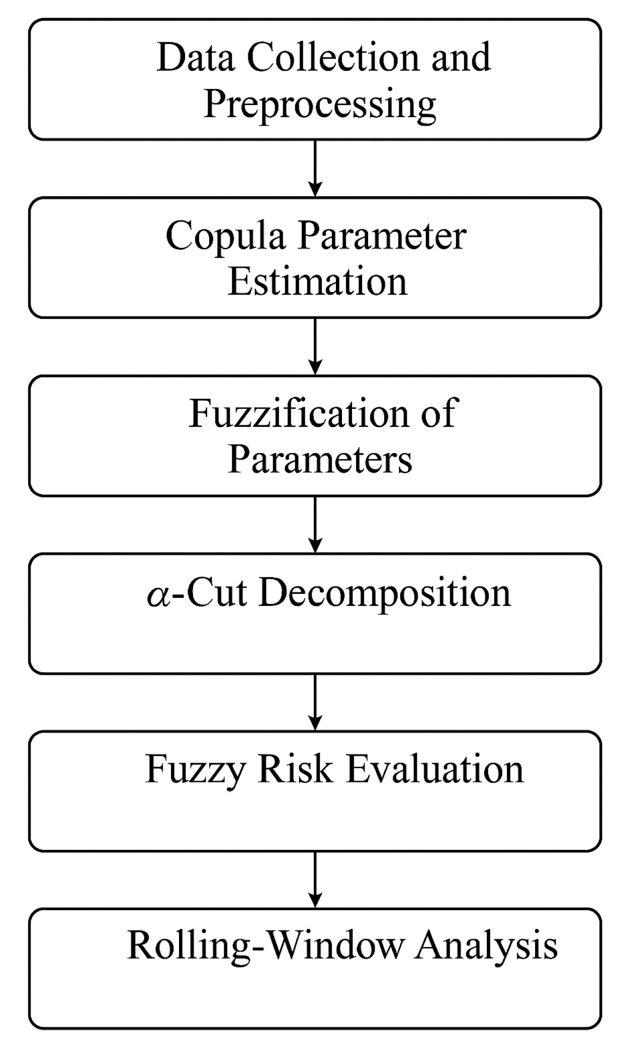
To summarize the framework’s structure, Figure 2 illustrates the main methodological steps.

The integration of both theoretical and empirical components strengthens the coherence of the study. After presenting the proposed fuzzy copula optimization framework in Section 4, Section 5 extends this framework to real financial data. The empirical applicability in capturing asymmetric and time-varying dependencies is thus highlighted. Section 4 and Section 5 ensure continuity between the model’s conceptual development and its real-world implementation.

4. Empirical Results

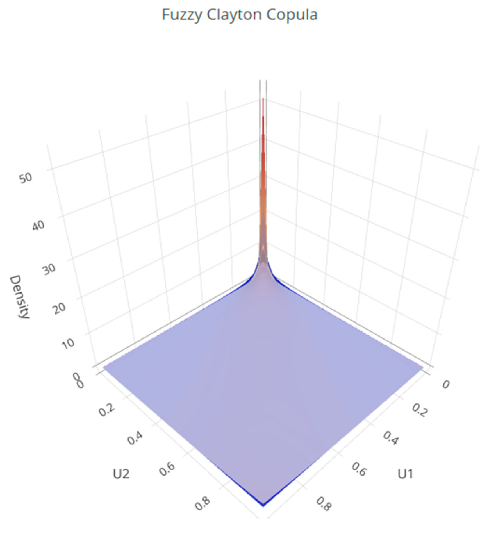
Figure 3 displays the theoretical dependence structure generated by the Fuzzy Clayton Copula. The orange surface corresponds to the upper α-cut (stronger lower-tail dependence), while the blue surface represents the lower α-cut (weaker dependence), illustrating the uncertainty associated with the fuzzy copula parameter. The sharp peak near the origin reflects the presence of strong lower-tail dependence, meaning that extreme joint realizations in the lower range of the distribution tend to occur simultaneously. This makes the Clayton copula suitable for capturing downside dependence structures in a fuzzy framework.

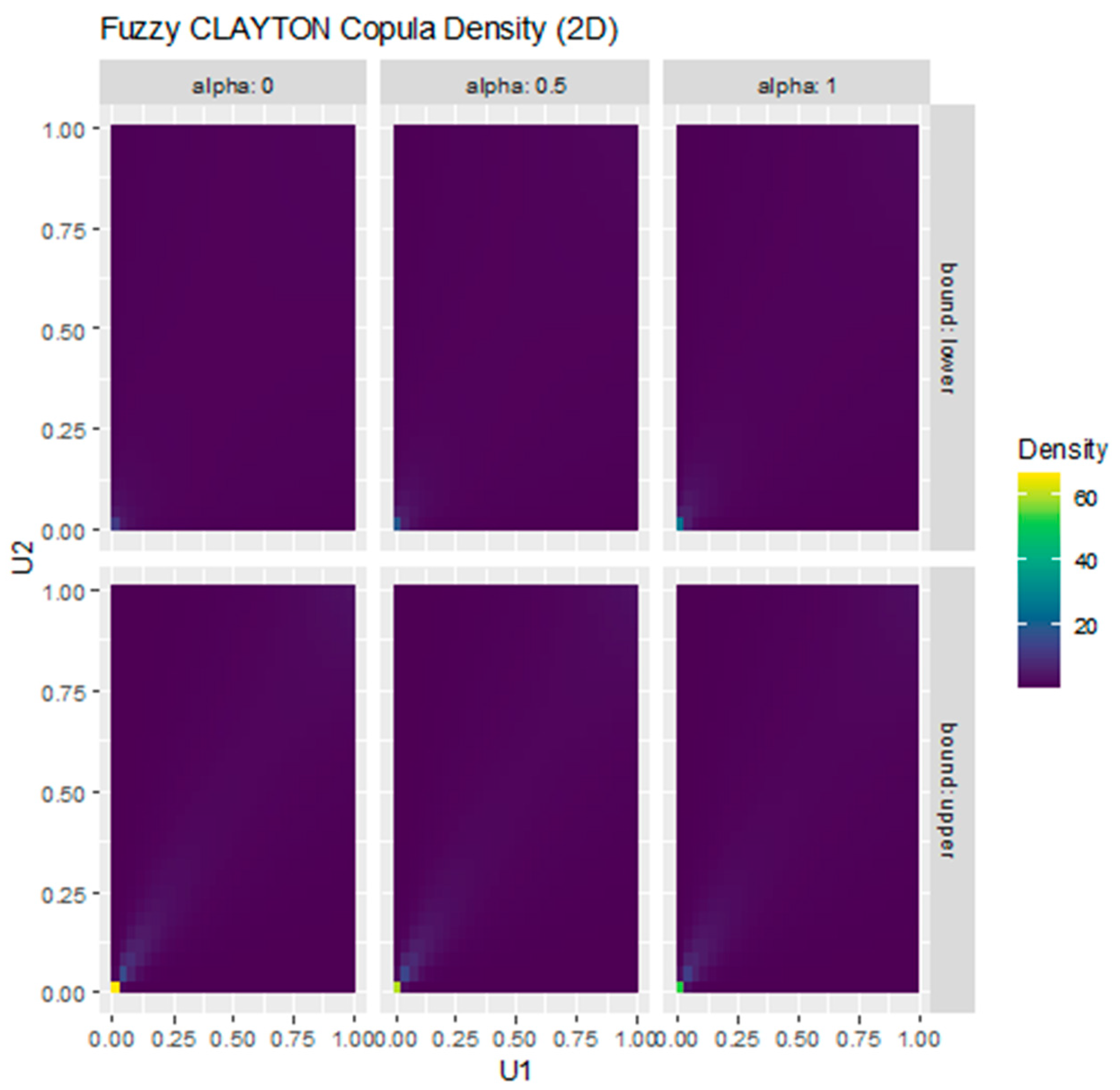
Figure 4 illustrates how the dependence structure of the Clayton copula evolves under fuzzification. The upper and lower bounds correspond to the α-cut intervals, while the panels for α = 0, 0.5, and 1 show how uncertainty around the copula parameter is progressively reduced. The concentration of density in the lower-left corner reflects the lower-tail dependence captured by the Clayton family.

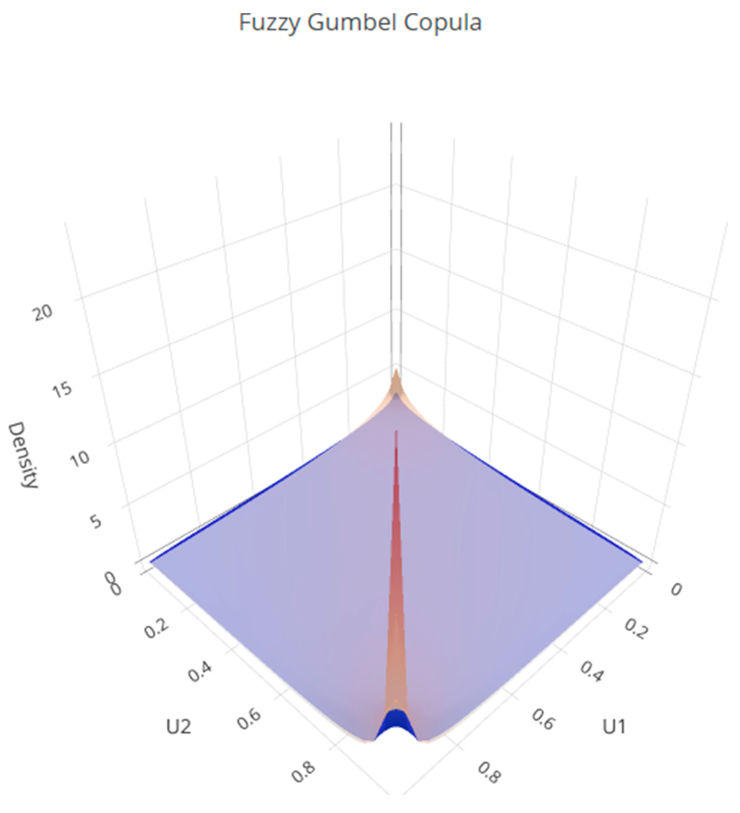
The surface in Figure 5 illustrates the dependence structure of the Gumbel copula under fuzzification. The orange surface shows the upper α-cut (stronger dependence), while the blue surface represents the lower α-cut (weaker dependence), capturing the uncertainty in the fuzzy copula parameter. The pronounced peak in the upper-right corner indicates strong upper-tail dependence, meaning that extreme joint realizations at high levels of the distribution tend to cluster together. This property makes the Gumbel copula particularly suitable for modeling co-movements during extreme positive outcomes.

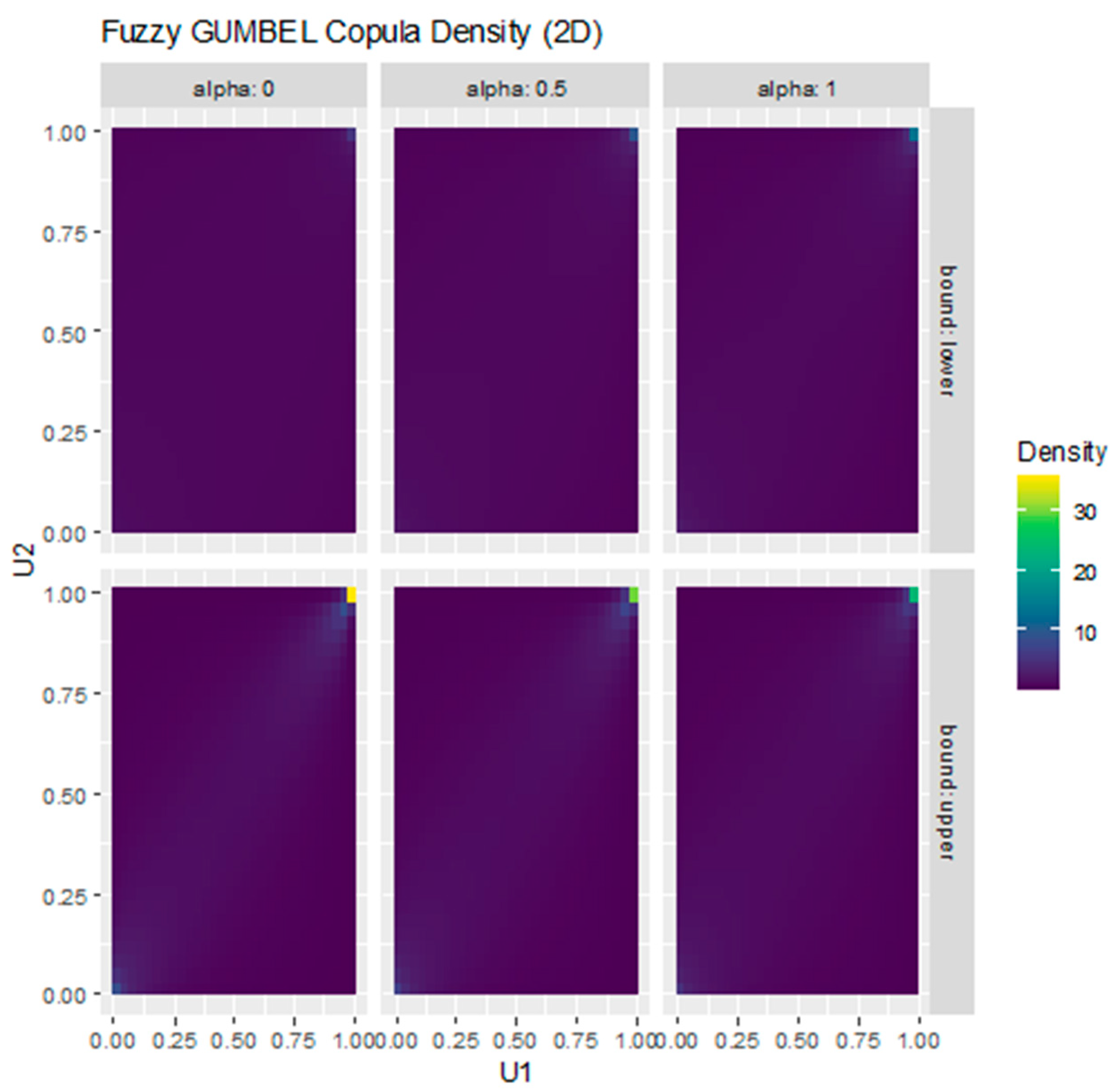
Figure 6 shows how the fuzzification of the Gumbel copula parameter translates into different dependence structures under α-cuts. The panels illustrate the lower and upper bounds of the fuzzy set for α = 0, 0.5, and 1. The concentration of density in the upper-right corner confirms the presence of upper-tail dependence, which becomes more evident as α increases and uncertainty is reduced.

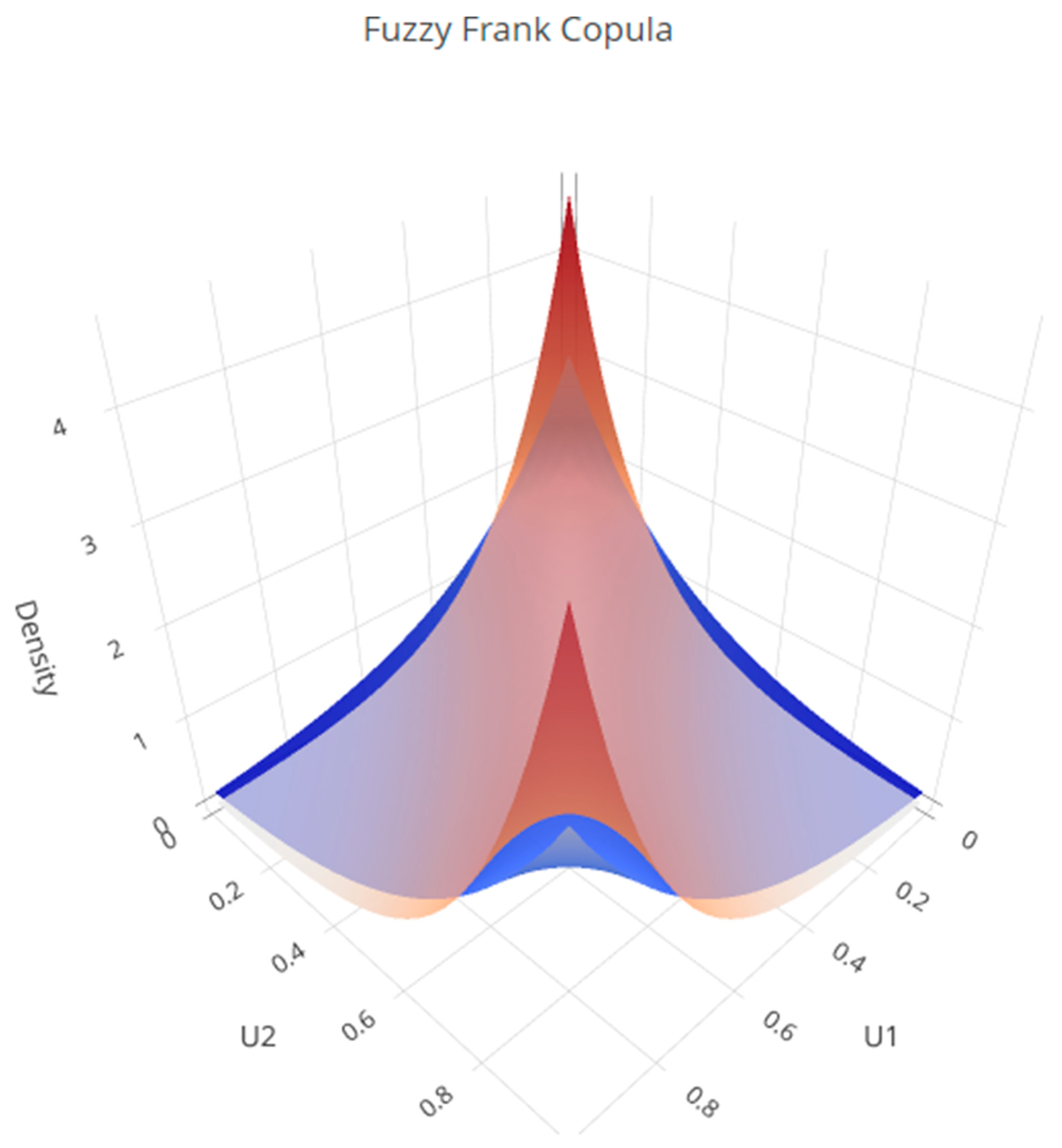
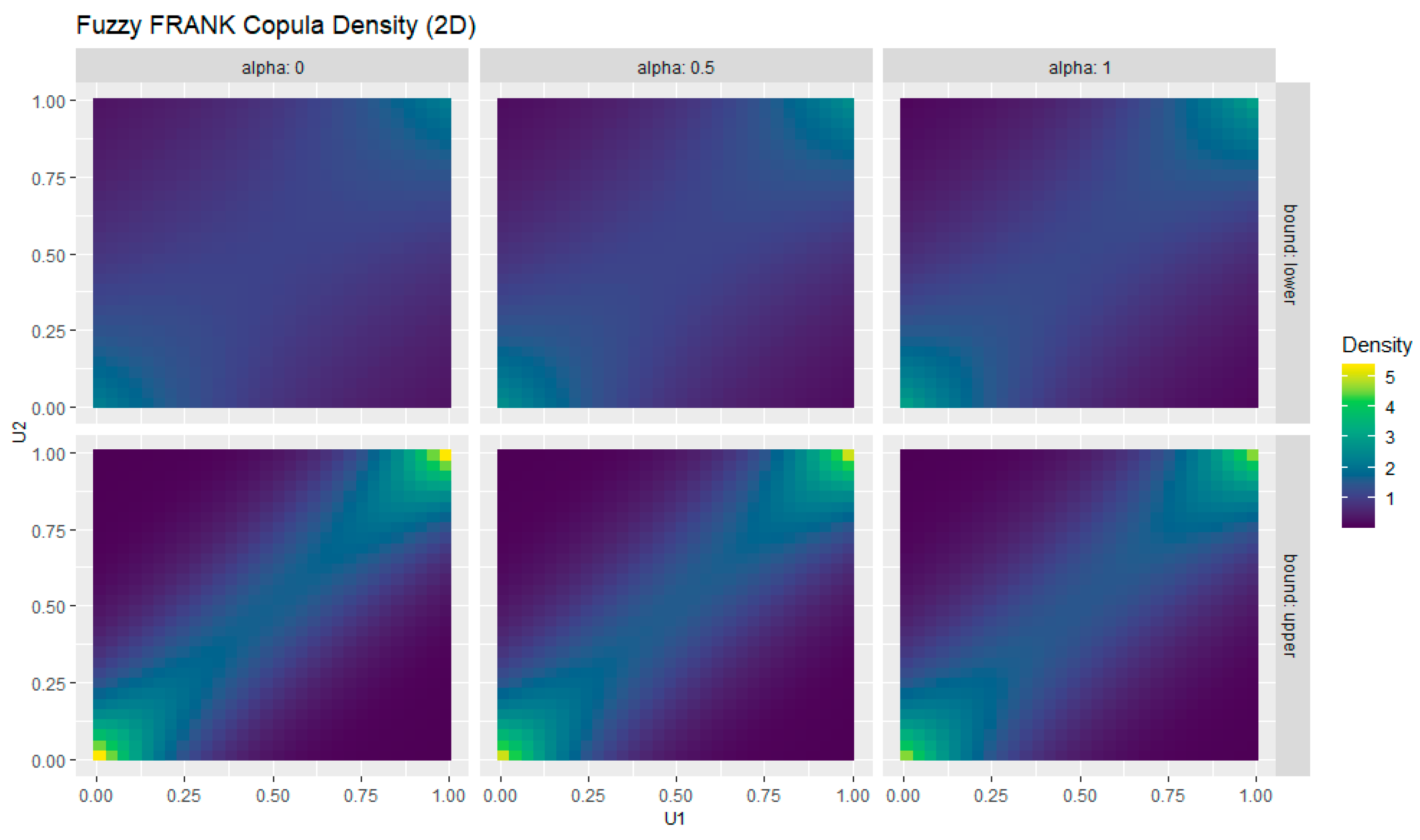
Figure 7 represents the dependence structure of the Frank copula under fuzzification. Unlike Clayton and Gumbel, the Frank copula is symmetric and does not exhibit tail dependence. The orange surface represents the upper α-cut (stronger dependence), while the blue surface corresponds to the lower α-cut (weaker dependence). The symmetric color pattern reflects the Frank copula’s balanced dependence structure, with fuzzification illustrating uncertainty in the copula parameter. The smooth surface highlights moderate dependence that is evenly distributed across the range of values, making the Frank copula suitable for capturing balanced, non-extreme associations between variables.

Figure 8 shows the effect of fuzzification on the Frank copula, represented through α-cuts at 0, 0.5, and 1. The lower and upper bounds illustrate the uncertainty range for the copula parameter, while the symmetric color patterns reflect the Frank copula’s balanced dependence structure. The absence of tail concentration confirms that this copula does not exhibit lower- or upper-tail dependence, but rather captures moderate dependence across the full distribution.

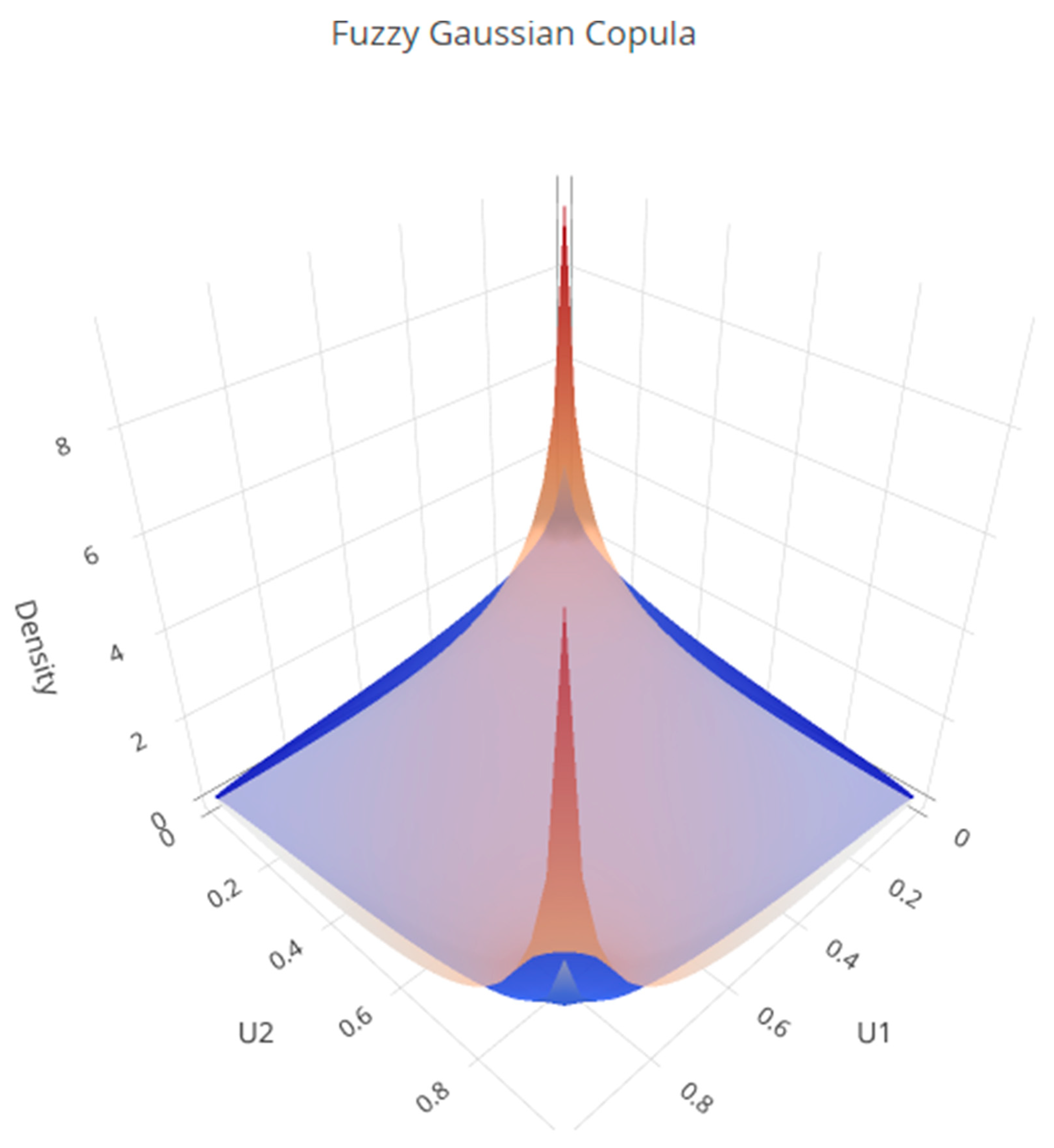
Figure 9 depicts the dependence structure of the Gaussian copula under fuzzification. The surface is symmetric and smooth, reflecting the absence of tail dependence. The Gaussian copula captures linear correlation across variables, with fuzzification introducing uncertainty around the correlation parameter. The orange surface represents the upper α-cut (stronger correlation), while the blue surface corresponds to the lower α-cut (weaker correlation). The color contrast visualizes the uncertainty in the fuzzy correlation parameter ρ, reflecting the symmetric dependence structure of the Gaussian copula. Unlike Clayton or Gumbel, this copula does not emphasize extreme co-movements but rather models average dependence in a flexible framework.

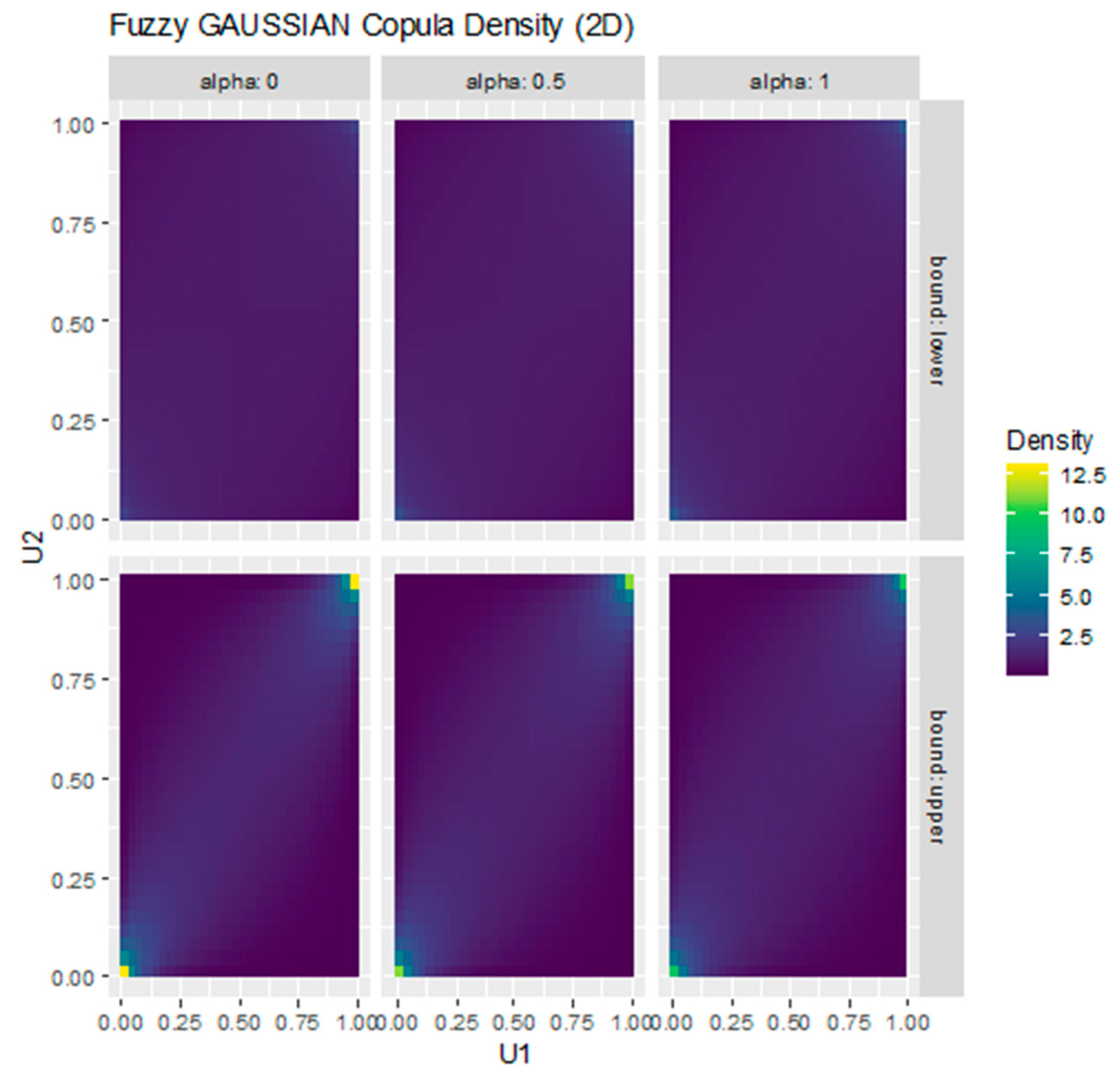
Figure 10 illustrates the Gaussian copula under fuzzification at α = 0, 0.5, and 1, with corresponding lower and upper bounds. The smooth and symmetric density patterns confirm the absence of tail dependence, in line with the theoretical properties of the Gaussian copula. The α-cut representation highlights how uncertainty in the correlation parameter is gradually reduced as α increases, leading to sharper dependence structures.

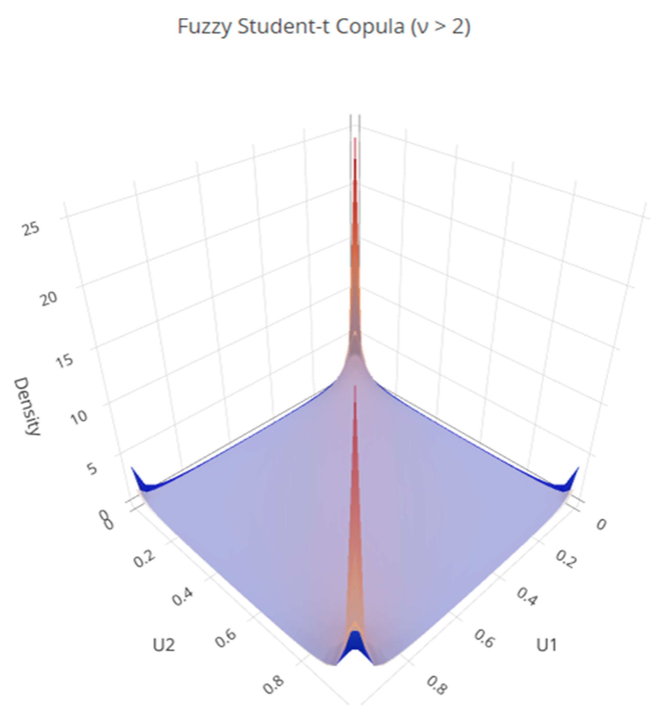
Figure 11 illustrates the dependence structure of the Student-t copula under fuzzification. The orange surface represents the upper α-cut (stronger dependence and heavier tails), while the blue surface corresponds to the lower α-cut (weaker dependence). The color contrast illustrates the uncertainty in the fuzzy parameters ρ and ν, highlighting the copula’s symmetric but tail-dependent structure. The surface shows strong concentration in both the lower-left and upper-right corners, reflecting the presence of tail dependence in both directions. This makes the Student-t copula particularly suitable for modeling joint extreme events, while the fuzzy framework captures parameter uncertainty in the degrees of freedom and correlation parameters.

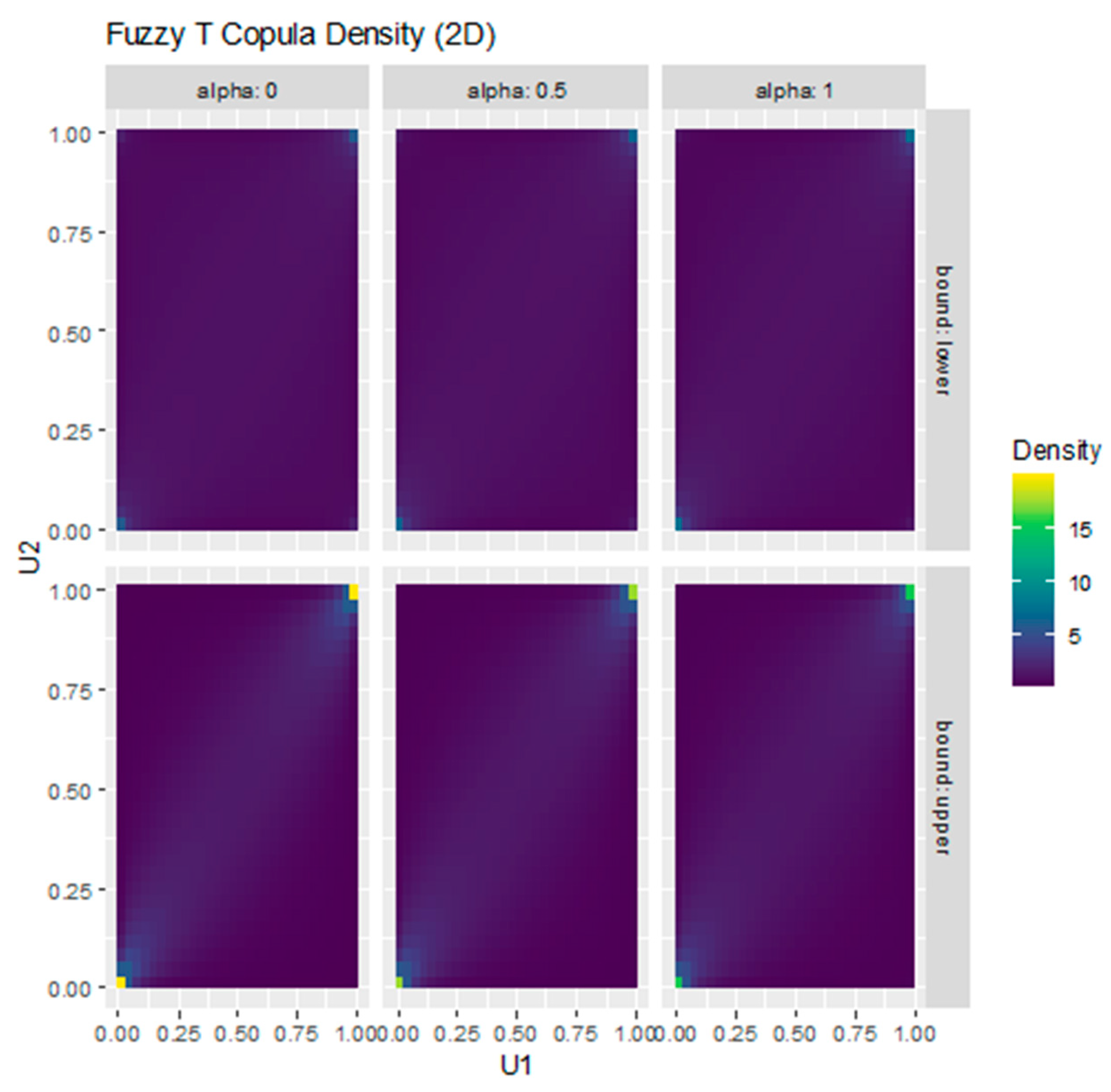
Figure 12 displays the Fuzzy Student-t copula under α-cuts (0, 0.5, and 1), with corresponding lower and upper bounds. The density patterns highlight the presence of both lower- and upper-tail dependence, consistent with the theoretical properties of the Student-t copula. As α increases, the parameter uncertainty narrows, producing sharper dependence structures that emphasize the copula’s ability to capture joint extreme events.

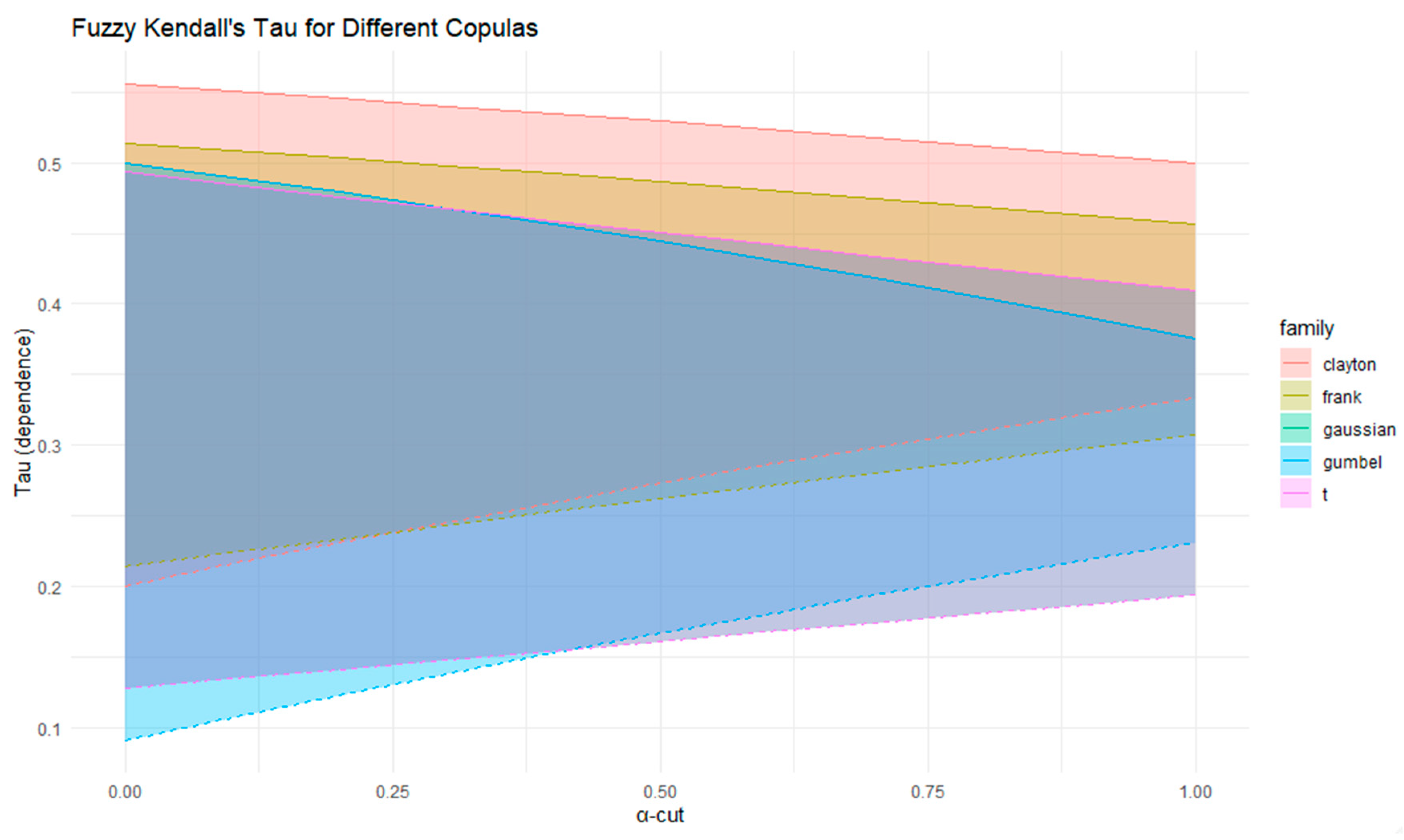
Figure 13 compares the evolution of fuzzy Kendall’s tau for five copula families (Clayton, Gumbel, Frank, Gaussian, and Student-t) as α varies from 0 to 1. The shaded areas represent the uncertainty intervals of dependence, which gradually shrink as α increases, reflecting reduced fuzziness in the copula parameters. The Clayton copula exhibits the strongest overall dependence, while the Gaussian and Student-t show weaker but more stable dependence. The Gaussian copula’s green area is visible but partially overlapped by the Gumbel region due to similar dependence structures.

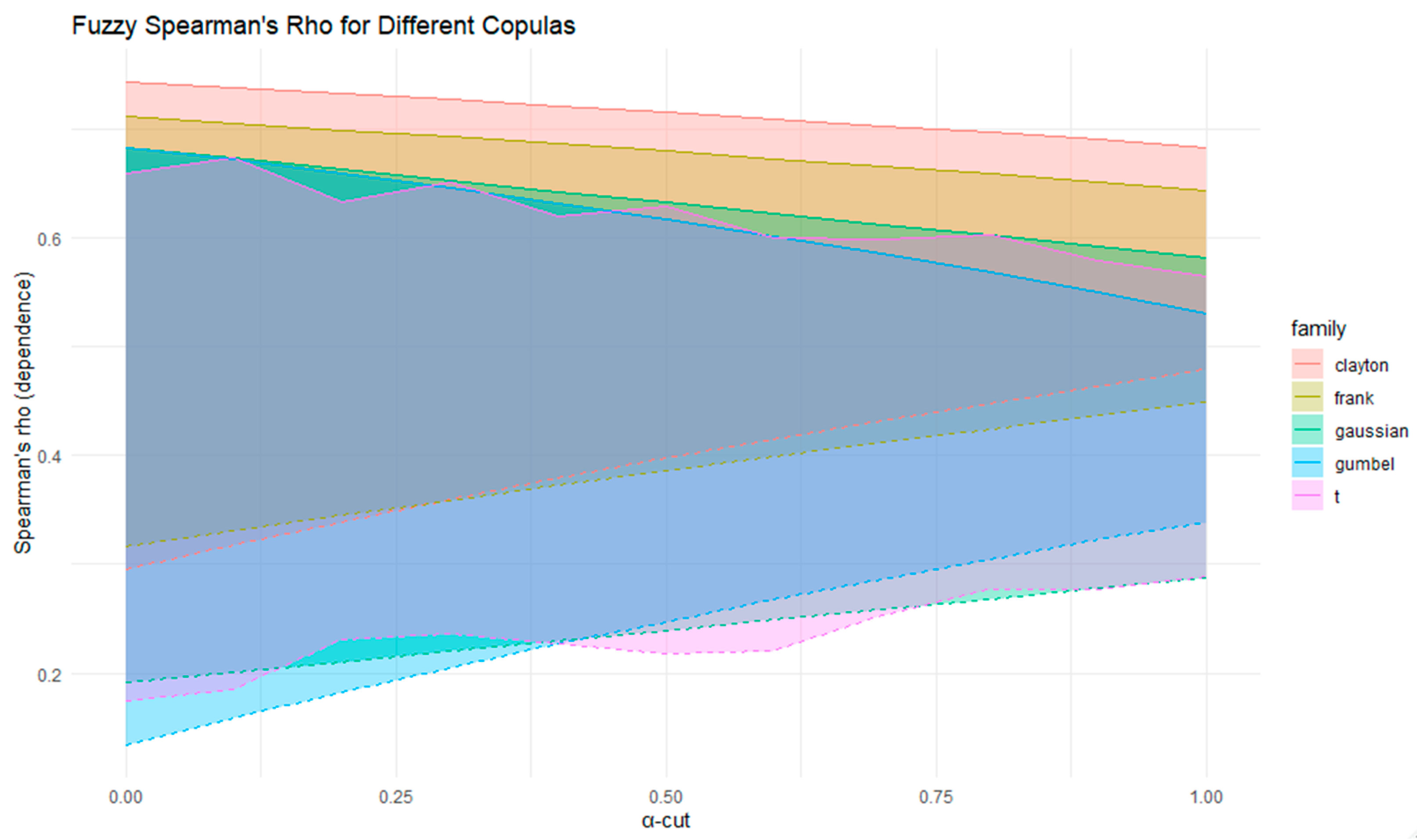
Figure 14 presents fuzzy Spearman’s rho values for the five copula families (Clayton, Gumbel, Frank, Gaussian, and Student-t) as α increases from 0 to 1. The shaded bands capture the uncertainty around dependence measures, which become narrower with higher α-cuts. Consistent with Kendall’s tau results, the Clayton copula shows the strongest monotonic dependence, while the Gaussian and Student-t exhibit more moderate dependence levels. This comparison confirms that fuzzification provides a richer representation of parameter uncertainty in rank-based dependence metrics.

Table 2. Fuzzy Kendall’s Tau and Spearman’s Rho for different copula families.

Family	Measure	Support Min	Support Max	Core Min	Core Max
Clayton	tau	0.2000000	0.5555556	0.3333333	0.5000000
Gumbel	tau	0.0990909	0.5000000	0.2307692	0.3750000
Frank	tau	0.2138946	0.5141736	0.3072470	0.4567010
Gaussian	tau	0.1281884	0.4936334	0.1939734	0.4096655
t	tau	0.1281884	0.4936334	0.1939734	0.4096655
Clayton	rho	0.2955286	0.7423365	0.4784902	0.6828928
Gumbel	rho	0.1341307	0.6828545	0.3389109	0.5296899
Frank	rho	0.3168216	0.7108174	0.4487150	0.6434871
Gaussian	rho	0.1913057	0.6829105	0.2875642	0.5819201
t	rho	0.2161297	0.6691901	0.2696605	0.5652711

reports the fuzzy dependence measures, Kendall’s Tau (τ) and Spearman’s Rho (ρ), for five copula families. The Clayton copula shows the strongest overall dependence, with τ and ρ values concentrated in higher ranges, confirming its suitability for modeling lower-tail risk. The Frank copula reveals moderate and symmetric dependence with relatively stable intervals, indicating a balanced association without tail asymmetry. Gumbel exhibits weaker average dependence but with wider uncertainty, reflecting its emphasis on upper-tail behavior. The Gaussian copula produces lower dependence levels, consistent with its linear structure and lack of tail dependence. The Student-t copula yields results close to the Gaussian but with slightly broader ranges, highlighting its additional flexibility in capturing both tails. Clayton and Frank provide the most consistent dependence structures, Gumbel emphasizes upper-tail risk under greater uncertainty, and Gaussian and Student-t suggest moderate to weaker associations.

The Gaussian copula produces lower dependence levels, consistent with its linear structure and lack of tail dependence. The Student-t copula yields results close to the Gaussian but with slightly broader ranges, highlighting its additional flexibility in capturing both tails. Clayton and Frank provide the most consistent dependence structures, Gumbel emphasizes upper-tail risk under greater uncertainty, and Gaussian and Student-t suggest moderate to weaker associations.

Table 3. α-cut parameter ranges for the five copula families.

Copula	Parameter	Support [a1, a4] (±20%)	Core [a2, a3] (±10%)	Tail Focus
Clayton	θ > 0	[0.8$\widehat{\theta }$, 1.2$\widehat{\theta }$]	[0.9$\widehat{\theta }$, 1.1$\widehat{\theta }$]	Lower-tail dependence
Gumbel	θ ≥ 1	[max (1, 0.8$\widehat{\theta }$), 1.2$\widehat{\theta }$]	[max (1, 0.9$\widehat{\theta }$), 1.1$\widehat{\theta }$]	Upper-tail dependence
Frank	θ ≠ 0	[0.8$\widehat{\theta }$, 1.2$\widehat{\theta }$]	[0.9$\widehat{\theta }$, 1.1$\widehat{\theta }$]	Symmetric
Gaussian	ρ ∈ [−0.99,0.99]	[$\widehat{\rho }$ − 0.2|$\widehat{\rho }$|, $\widehat{\rho }$ + 0.2|$\widehat{\rho }$|]	[$\widehat{\rho }$ − 0.1|$\widehat{\rho }$|, $\widehat{\rho }$ + 0.1|$\widehat{\rho }$|]	Symmetric
t	ρ ∈ [−0.99,0.99], ν = 5	[$\widehat{\rho }$ − 0.2|$\widehat{\rho }$|, $\widehat{\rho }$ + 0.2|$\widehat{\rho }$|]	[$\widehat{\rho }$ − 0.1|$\widehat{\rho }$|, $\widehat{\rho }$ + 0.1|$\widehat{\rho }$|]	Both tails

and

Table 4. Tail-dependence coefficients under α-cuts.

Copula	${\mathit{\lambda }}_{\mathit{L}}$	${\mathit{\lambda }}_{\mathit{U}}$	Range (α = 0 → 1)
Clayton	$2^{-1/{\theta }_{\alpha }}$	0	≈0.18–0.33
Gumbel	0	$2-2^{-1/{\theta }_{\alpha }}$	≈0.22–0.36
Frank	0	0	0
Gaussian	0	0	0
t	$2t_{\nu +1}(-\sqrt{{\displaystyle \frac{(\nu +1)(1-{\rho }_{\alpha })}{1+{\rho }_{\alpha }}}}$)	$2t_{\nu +1}(-\sqrt{{\displaystyle \frac{(\nu +1)(1-{\rho }_{\alpha })}{1+{\rho }_{\alpha }}}}$)	≈0.07–0.10 (ν = 5)

report the α-cut parameter ranges and the associated lower- and upper-tail dependence coefficients $({\lambda }_L,{\lambda }_U)$ for the selected copula families, derived according to Demarta and McNeil (2005) [32], showing that only the Clayton, Gumbel, and Student-t copulas exhibit significant tail dependence.

Before applying fuzzification, we evaluated the adequacy of the five copula families using maximum-likelihood estimation and formal goodness-of-fit diagnostics.

Table 5. Copula model selection and goodness-of-fit statistics before fuzzification (Gold–Oil dependence).

Family	logLik	AIC	BIC	White p	PIT p
Clayton	11.7927	−21.5853	−15.7561	0.01	0.00
Gumbel	20.2719	−38.5439	−32.7146	0.00	0.00
Frank	10.1309	−18.2617	−12.4325	0.00	0.00
Gaussian	10.9082	−19.8163	−13.9871	0.00	0.00
t	35.2506	−68.5013	−62.6720	0.15	0.00

reports the log-likelihood, Akaike and Bayesian Information Criteria (AIC, BIC), and two complementary GOF tests: White’s information-matrix test and a probability-integral-transform (PIT) Kolmogorov–Smirnov test. The Student-t copula achieved the lowest AIC/BIC and the highest White p-value, indicating superior fit and heavy-tailed dependence consistent with empirical risk behavior. Nevertheless, the Gaussian copula displayed the broadest fuzzy dependence range, consistent with its conservative risk interpretation.

5. Case Study

To empirically validate the proposed fuzzy copula framework, a case study is conducted on the Gold–Oil portfolio over the period 1 January 2015 to 1 January 2025. The data consist of daily closing prices for gold futures (symbol GC = F) and crude oil futures (symbol CL = F), retrieved from Yahoo Finance and converted into continuously compounded daily returns. The choice of these two assets is motivated by their fundamental economic interconnection—gold serving as a safe-haven asset and oil as a key indicator of global economic activity. This makes them a benchmark for studying nonlinear dependence and asymmetry in commodity markets.

The empirical analysis applies several copula families (Clayton, Gumbel, Frank, Gaussian, and Student-t) to model dependence under fuzzified parameter uncertainty. Fuzzy VaR and CVaR are then computed for the portfolio, incorporating α-cut decomposition to represent uncertainty intervals for potential losses. A rolling-window approach with a 250-day window and a 50-day step size captures the evolution of fuzzy dependence and risk over time, allowing for the detection of structural changes and crisis-induced tail events. This case study thus proves how the integration of fuzziness and temporal dynamics enhances the interpretability of copula-based risk assessment in financial markets.

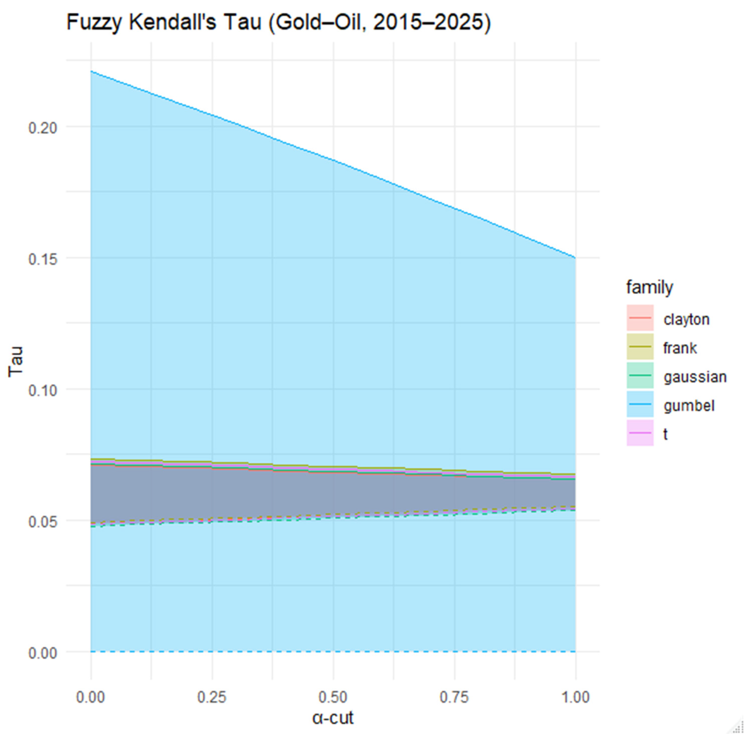
Figure 15 illustrates the fuzzy Kendall’s Tau estimates for the dependence structure between gold and oil returns over the period 1 January 2015–1 January 2025, evaluated across different α-cuts and copula families. The shaded regions represent the range of possible dependence values, with the core indicating the most plausible levels. The Gaussian copula shows the widest fuzzy interval, suggesting higher uncertainty in capturing the association. By contrast, the Clayton, Frank, Gumbel, and Student-t copulas produce narrower and more stable ranges, indicating weaker but more consistent dependence. The results point to a relatively low degree of association between gold and oil returns, with the strongest but most uncertain values arising under the Gaussian copula specification.

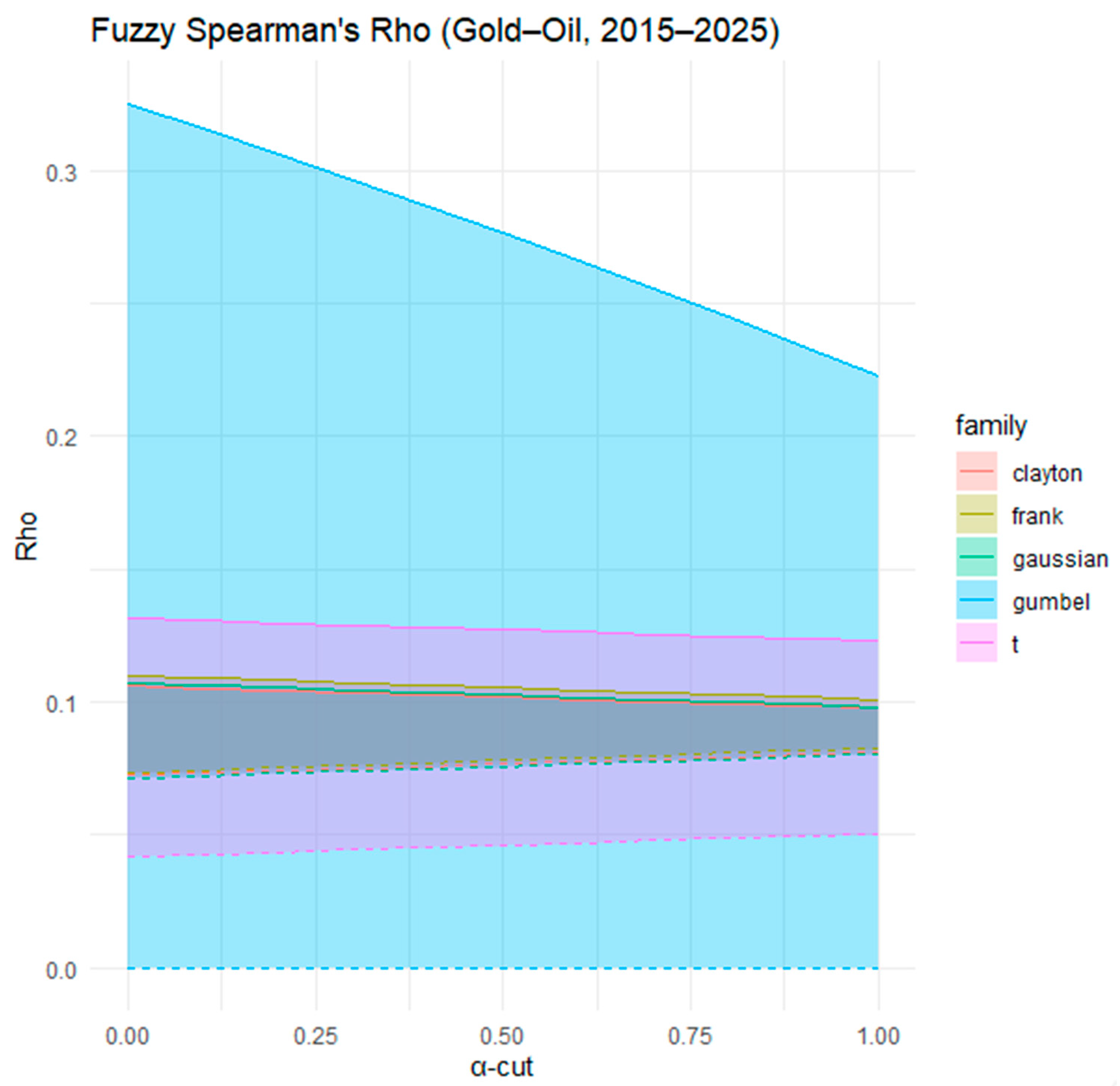
Figure 16 shows the fuzzy Spearman’s Rho estimates for the dependence between gold and oil returns from 1 January 2015–1 January 2025 across α-cuts and copula families. The Gaussian copula again generates the widest fuzzy interval, reflecting a higher level of uncertainty in modeling the relationship. The other copulas, including Clayton, Frank, Gumbel, and Student-t, remain closer together with relatively narrow ranges, indicating a weak but stable dependence. Compared with Kendall’s Tau, the Spearman’s Rho estimates highlight the same pattern of low overall association, with Gaussian suggesting the upper bound of possible dependence, while the others converge toward weaker values. This suggests that gold and oil returns exhibit only modest concordance, with little evidence of strong nonlinear dependence.

Table 6. Fuzzy Copula Dependence Measures (Gold–Oil, 1 January 2015–1 January 2025).

Family	Measure	Support Min	Support Max	Core Min	Core Max
Clayton	tau	0.04841408	0.07090472	0.05413820	0.06538232
Gumbel	tau	0.00000000	0.22070425	0.00000000	0.14985918
Frank	tau	0.04909143	0.07345835	0.05519927	0.06738880
Gaussian	tau	0.04765030	0.07155933	0.05361992	0.06557390
t	tau	0.04824385	0.07243929	0.05427804	0.06637970
Clayton	rho	0.07247134	0.10606828	0.08102522	0.09783242
Gumbel	rho	0.00000000	0.32492514	0.00000000	0.22242903
Frank	rho	0.07358919	0.11002667	0.08273072	0.10095159
Gaussian	rho	0.07142538	0.10716933	0.08035853	0.09823031
t	rho	0.04183374	0.13161862	0.05061031	0.12290416

reports the fuzzy copula dependence measures between gold and oil over the period 1 January 2015–1 January 2025, expressed through Kendall’s Tau and Spearman’s Rho. The findings reveal that the overall dependence is weak and relatively stable across all copula families. For Kendall’s Tau, the Clayton, Frank, Gaussian, and Student-t copulas exhibit similarly low and consistent values, indicating limited concordance between the two markets. In contrast, the Gumbel copula suggests a wider range of uncertainty, consistent with its upper-tail sensitivity and capacity to capture asymmetric dependence. Regarding Spearman’s Rho, the Clayton copula yields the most stable and narrow estimates, while Gumbel again introduces greater variability, reflecting fluctuations in extreme co-movements. The Frank, Gaussian, and Student-t copulas provide overlapping and moderate dependence values, confirming the weak but persistent association between gold and oil.

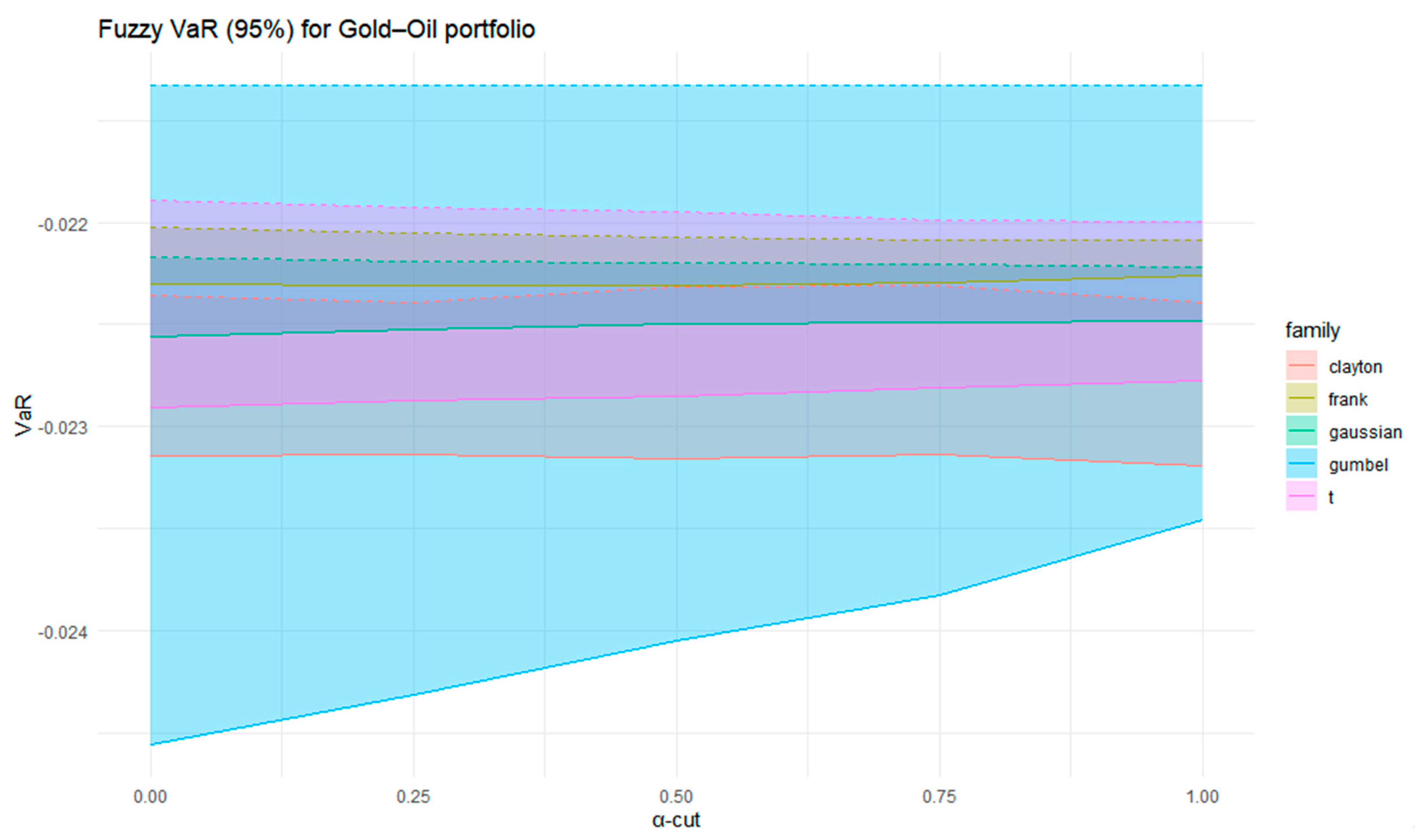
Figure 17 presents the fuzzy 95% VaR for the Gold–Oil portfolio estimated across various copula families and α-cuts. The shaded regions depict the fuzzy uncertainty intervals associated with parameter imprecision. Among the copulas, the Gaussian exhibits the broadest fuzzy range, indicating the highest level of uncertainty and the most conservative risk assessment. The Gumbel copula also captures a relatively wide range of potential losses, consistent with its sensitivity to upper-tail dependence. In contrast, the Clayton, Frank, and Student-t copulas yield narrower and more stable VaR intervals, implying more concentrated and predictable risk profiles. Across all families, the VaR estimates remain negative, reflecting potential downside losses at the 95% confidence level.

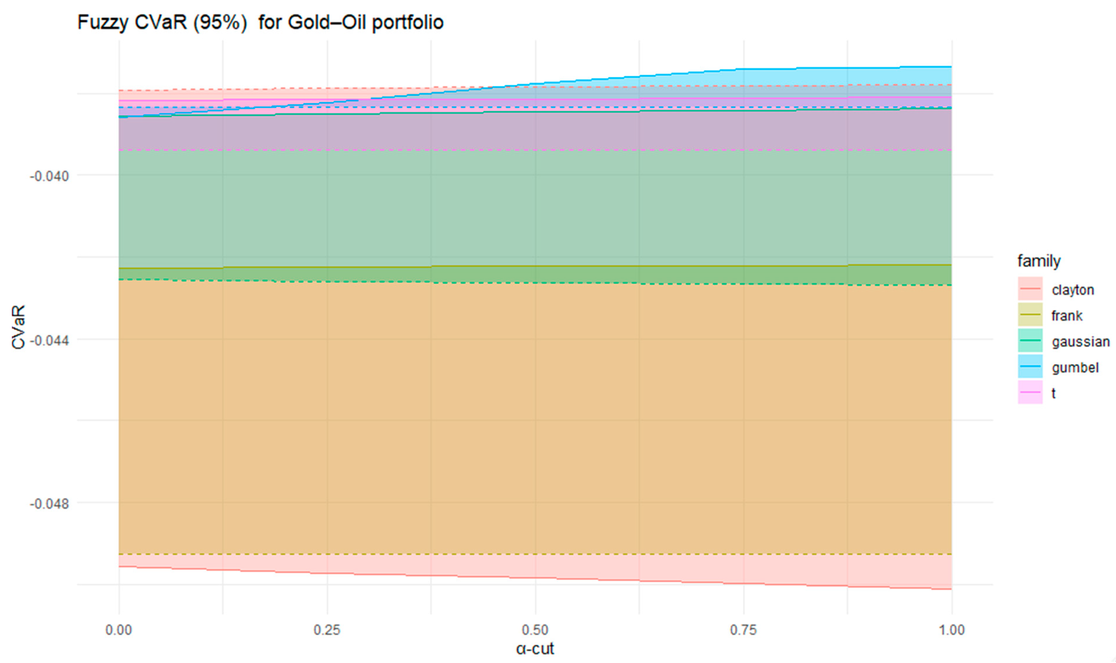
Figure 18 presents the fuzzy 95% CVaR for the Gold–Oil portfolio estimated across different copula families and α-cuts. In contrast to VaR, which captures only the quantile of extreme losses, CVaR measures the expected shortfall beyond that quantile, providing a more comprehensive view of downside risk. The results reveal notable heterogeneity among copula families. The Clayton copula produces the deepest losses for certain α-cuts, reflecting its strong lower-tail dependence and yielding the most conservative risk estimates. The Gaussian and Student-t copulas occupy an intermediate position, balancing linear dependence with moderate tail effects. Frank and Gumbel exhibit narrower and more stable CVaR intervals, implying smoother and less extreme risk behavior. The fuzzy CVaR results confirm that dependence structure is important in shaping tail risk assessments, with the Clayton and Student-t copulas emphasizing higher potential downside exposures.

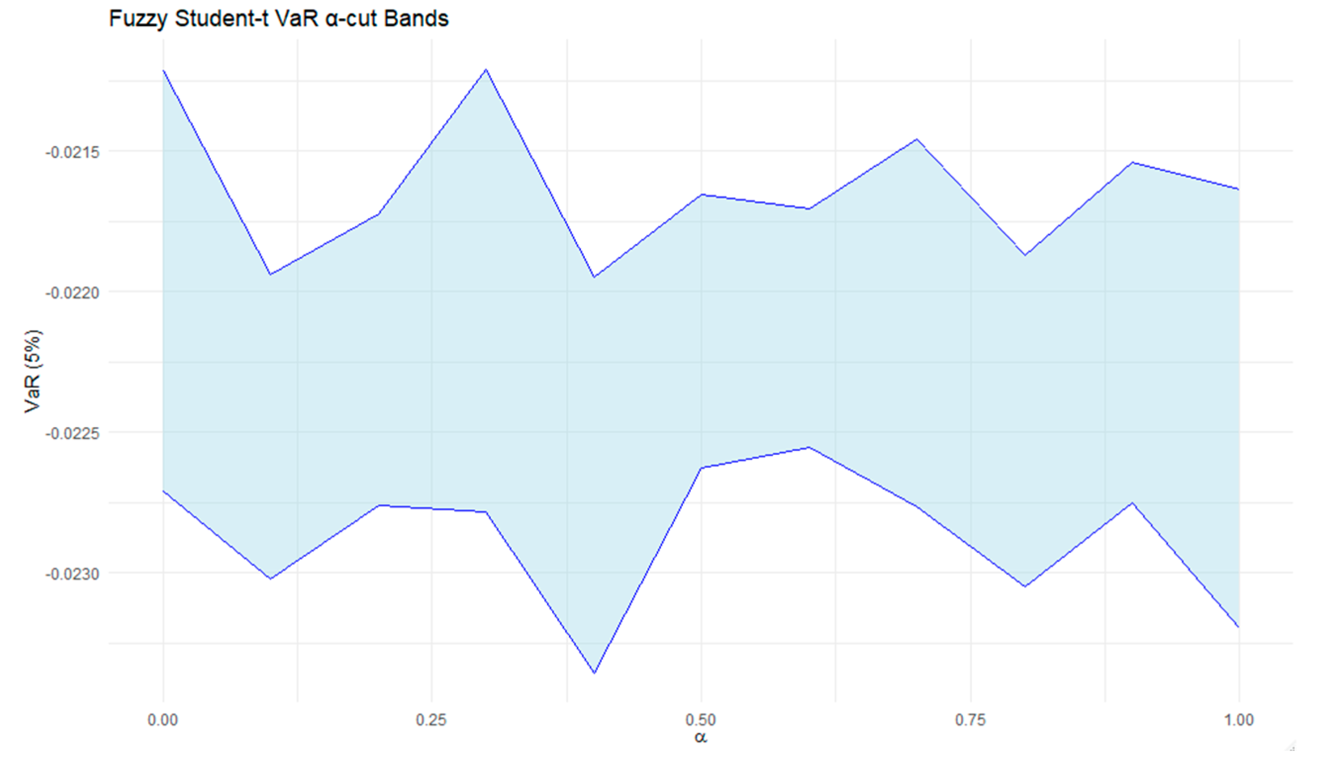
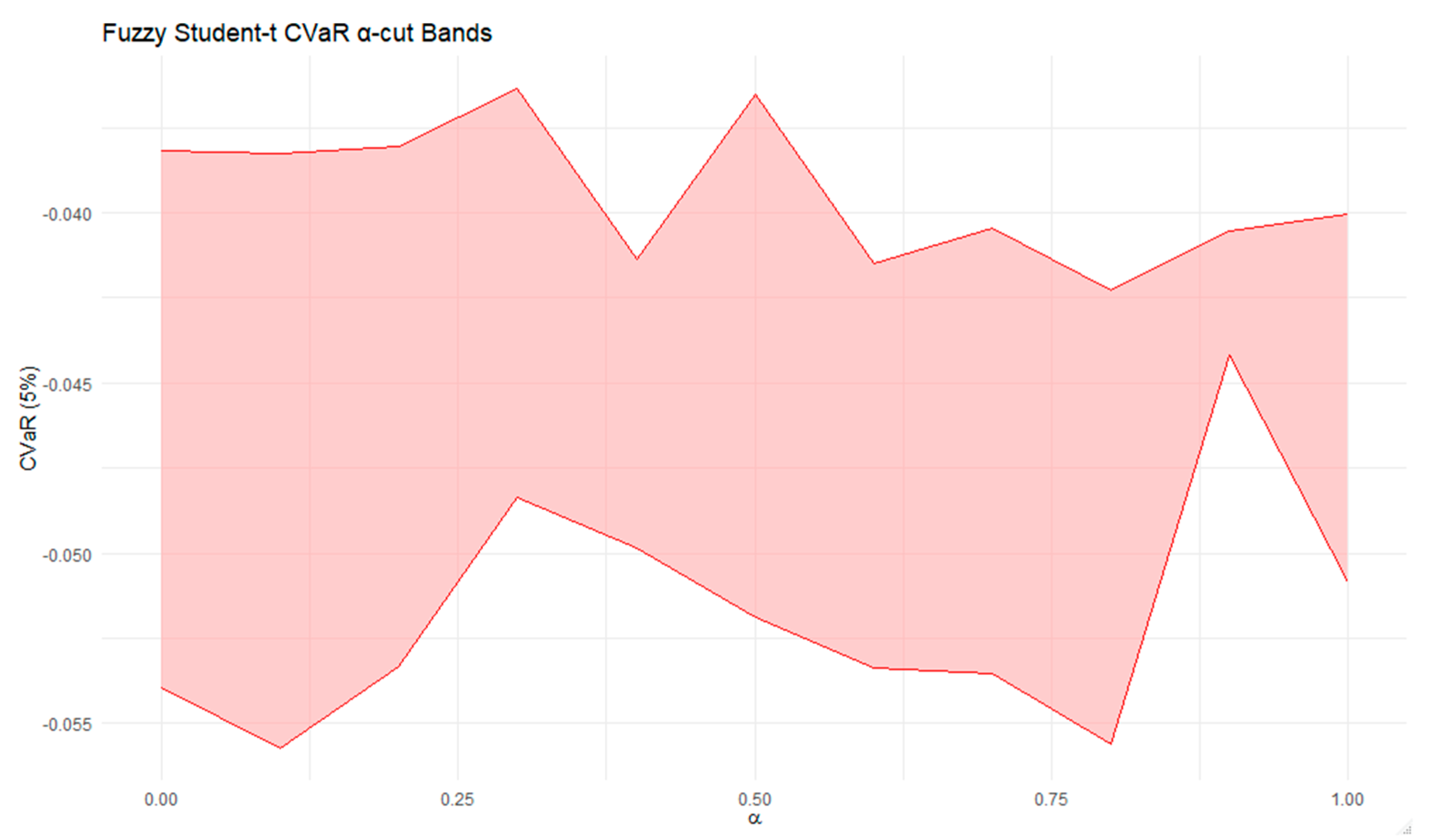
Figure 19 and Figure 20 illustrate the fuzzy α-cut envelopes of VaR and CVaR for the Student-t copula, computed using a seven-point interior grid within each α-cut interval $\left[{\nu }_L\left(\alpha \right),{\nu }_U\left(\alpha \right)\right]$. The smooth but bounded ribbons confirm that the fuzzy lower and upper limits accurately capture the full range of potential risk outcomes. Minor non-monotonic fluctuations across α-cuts reflect the joint influence of correlation and degrees of freedom on tail behavior. For the Gaussian, Clayton, Gumbel, and Frank copulas, VaR and CVaR vary monotonically with the dependence parameter, so for them no interior-grid evaluation is required.

Table 7. Fuzzy Value-at-Risk (VaR) and Conditional Value-at-Risk (CVaR) at 95% Confidence Level for the Gold–Oil Portfolio across Copula Families.

Family	VaR Support	VaR Core	CVaR Support	CVaR Core
Clayton	−0.0224 to −0.0231	−0.0224 to −0.0232	−0.0379 to −0.0496	−0.0378 to −0.0501
Gumbel	−0.0213 to −0.0246	−0.0213 to −0.0235	−0.0383 to −0.0386	−0.0383 to −0.0374
Frank	−0.0220 to −0.0223	−0.0221 to −0.0223	−0.0493 to −0.0423	−0.0493 to −0.0422
Gaussian	−0.0222 to −0.0226	−0.0225 to −0.0225	−0.0426 to −0.0386	−0.0427 to −0.0384
t	−0.0219 to −0.0229	−0.0220 to −0.0228	−0.0394 to −0.0382	−0.0394 to −0.0381

presents the fuzzy estimates of the VaR and CVaR for the Gold–Oil portfolio, including both support and core intervals across copula families. The results indicate that all VaR values are consistently negative, confirming potential portfolio losses at the 95% confidence level. The Clayton copula yields relatively stable VaR estimates, whereas Gumbel displays a wider dispersion, reflecting its sensitivity to upper-tail dependence. Frank and Gaussian copulas produce comparable and narrow VaR intervals, pointing to moderate and stable risk levels, while the Student-t copula yields similar outcomes to the Gaussian but with heavier tails incorporated.

Regarding CVaR, which captures the expected loss beyond the VaR threshold, all copulas reveal more pronounced downside risk, as theoretically expected. The Clayton and Student-t copulas exhibit the deepest CVaR intervals, emphasizing their ability to reflect stronger tail co-movements. The Gumbel copula again introduces broader variability, consistent with its asymmetric tail sensitivity, whereas the Frank and Gaussian copulas present smoother and less extreme risk profiles.

Although the Gaussian copula has no tail dependence, it is described in this study as “most conservative” in the sense of epistemic conservatism rather than aleatory tail risk (Zhou et al., 2023 [4]). The wider fuzzified intervals in Figure 15, Figure 16, Figure 17 and Figure 18 and Table 7 indicate greater parameter uncertainty (epistemic width of α-cut bands) rather than stronger tail co-movement. The Gaussian copula produces the broadest fuzzy VaR and CVaR ranges because its dependence structure, being symmetric and linear, does not anchor extreme events to either tail, allowing parameter uncertainty to propagate more widely through the fuzzy simulation. By contrast, the Student-t copula exhibits narrower but deeper tail losses, representing aleatory conservatism driven by heavy-tailed behavior. Therefore, “conservative” in the Gaussian case refers to the interval width of uncertainty, not to tail severity, which is captured instead by the Student-t and Clayton copulas. This interpretation aligns with the fuzzy VaR and CVaR bands in Figure 17 and Figure 18, where the Gaussian intervals are widest, while the Student-t bands extend further into the negative tail.

The results from Table 6 and Table 7 jointly illustrate how the strength and asymmetry of dependence influence portfolio risk under fuzziness. The weak fuzzy dependence observed across most copula families translates into bounded but asymmetric tail risk in Table 7. Specifically, while the overall concordance between gold and oil remains limited, copulas with stronger tail sensitivity—such as Gumbel (upper tail) and Clayton (lower tail)—generate wider and more uncertain fuzzy ranges for VaR and CVaR. This correspondence highlights that even modest dependence, when combined with tail asymmetry, can substantially affect the extent of downside exposure, reinforcing the importance of accurate copula selection in fuzzy portfolio risk modeling.

6. Rolling Window

To capture the temporal evolution of risk and dependence, a rolling-window framework is employed. This approach allows for dynamic assessment of fuzzy VaR and CVaR over time, reflecting changes in market conditions and tail behavior. Rolling windows are essential in financial risk modeling because they reveal how dependence structures and loss distributions shift during periods of stress and recovery. By applying a 250-day rolling window with a 50-day step, the analysis tracks how fuzzy copula-based risk measures evolve, uncovering both persistent and transient patterns of downside exposure. This dynamic perspective enhances the robustness of the fuzzy copula framework by integrating time variation with parameter uncertainty.

To ensure numerical precision, each window involves 10,000 Monte Carlo draws, and Monte Carlo standard errors (MCSEs) are computed for both VaR and CVaR. The mean MCSE represents only about 1.7% of the estimated risk metrics, confirming that simulation noise is negligible relative to fuzzy uncertainty.

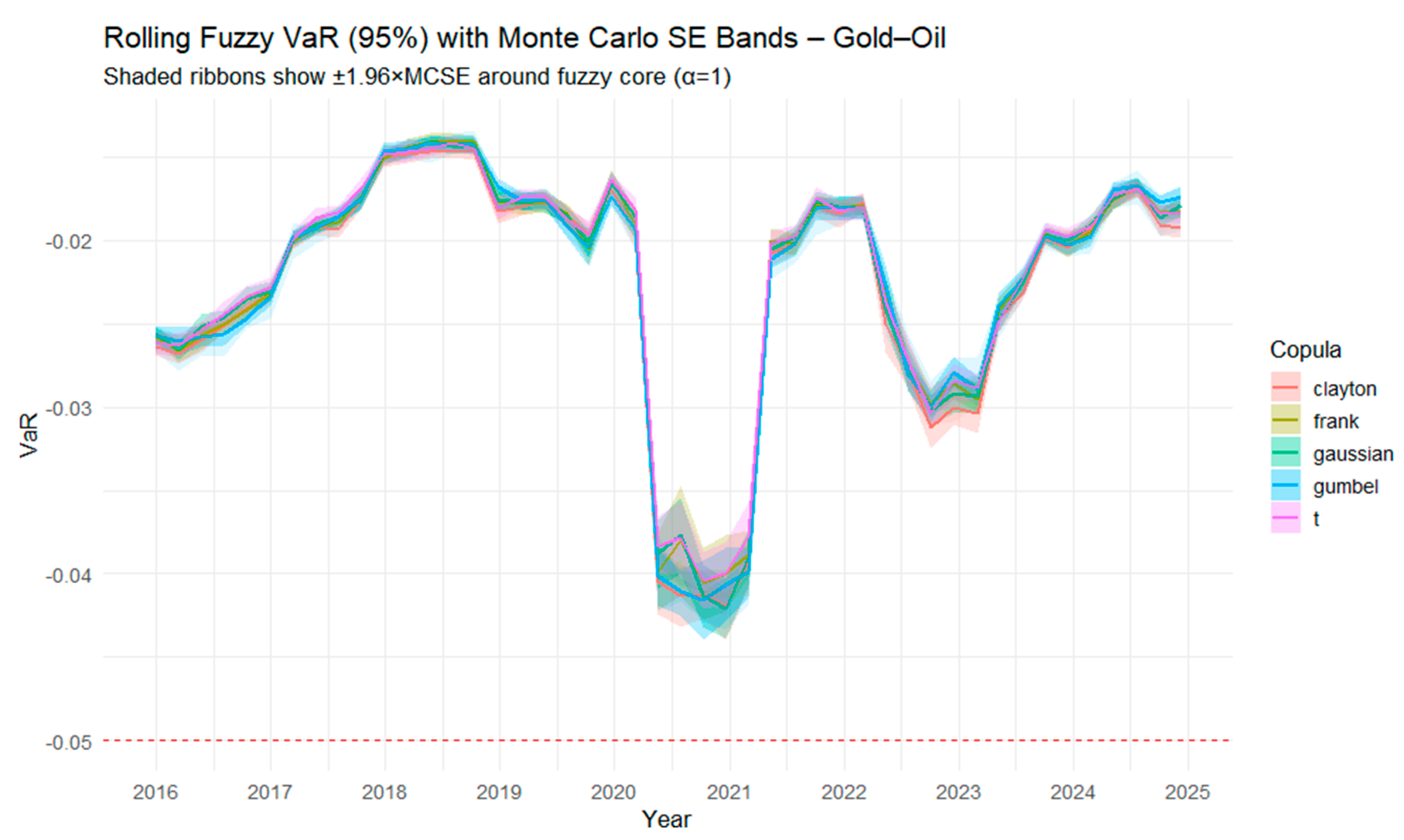
Figure 21 presents the time-varying fuzzy 95% VaR for the Gold–Oil portfolio, estimated with multiple copula families over a rolling window. The results reveal pronounced shifts in portfolio risk over time, with sharp declines around 2020–2021 corresponding to market turbulence, followed by periods of recovery and subsequent volatility episodes. Despite differences in tail behavior, the copula families generate broadly similar trajectories, indicating robustness of the fuzzy VaR estimates across dependence structures. The clustering of the lines suggests that while fuzziness introduces variability, the overall risk dynamics are consistent: losses deepen during global stress periods and ease in more stable market phases. The narrow Monte Carlo SE bands confirm that this time variation reflects genuine changes in dependence and tail behavior rather than simulation noise, reinforcing the robustness of the fuzzy copula–based risk estimates.

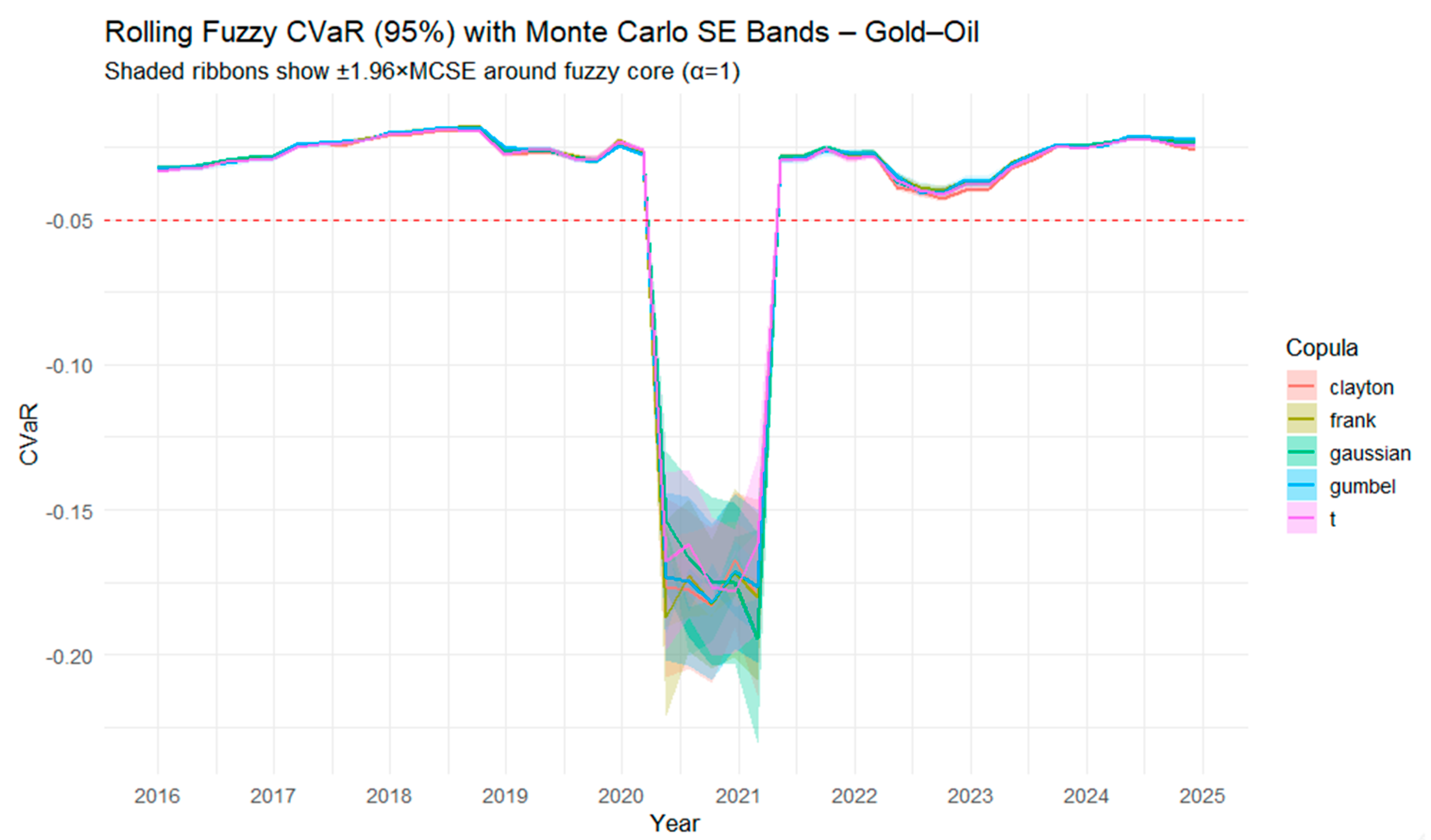
Figure 22 illustrates the evolution of fuzzy CVaR at the 95% confidence level for the Gold–Oil portfolio using different copula families. Shaded ribbons show ±1.96×MCSE around the fuzzy core (α = 1). The red dashed line indicates the zero-CVaR threshold, distinguishing loss regions (below the line) from neutral or non-loss regions (above the line). Compared with fuzzy VaR (Figure 21), CVaR highlights the severity of losses in the tail of the distribution. The results show that during stable periods, CVaR estimates remain relatively close across copulas, reflecting consistent moderate risk. However, during the 2020–2021 market turmoil, all copulas capture a pronounced deepening of downside risk, with CVaR values dropping sharply and exhibiting greater dispersion across families. This indicates that tail dependence plays a critical role under extreme stress, with the Student-t and Gumbel copulas showing stronger sensitivity to extreme losses. Post-2021, CVaR levels stabilize again, mirroring the recovery observed in VaR but with persistently wider risk margins. Rolling fuzzy CVaR complements fuzzy VaR by revealing not only the likelihood but also the magnitude of potential extreme losses, making it a more conservative and informative risk measure in turbulent markets. Monte Carlo precision diagnostics confirm that simulation noise is negligible. The mean MC standard error represents only about 2.1% of the absolute CVaR magnitude. The ±1.96 × MCSE bands are therefore almost indistinguishable at the plotted scale, verifying that the observed variation in fuzzy CVaR reflects genuine changes in dependence and tail behavior rather than stochastic noise.

Next, we make a comparison between Figure 21 and Figure 22. Rolling fuzzy VaR (Figure 21) captures the potential losses at the 95% confidence level, while rolling fuzzy CVaR (Figure 22) reflects the expected severity of losses beyond the VaR threshold.

The results highlight several important contrasts. First, both measures identify similar temporal patterns, with periods of relative stability (2016–2019, 2022–2025) and a sharp risk escalation during the 2020–2021 crisis. However, CVaR consistently produces more negative values than VaR, emphasizing its conservative nature by accounting for the full tail of the distribution rather than a single quantile.

Second, the divergence between copula families is more evident in CVaR. While VaR estimates across copulas largely converge during tranquil periods, CVaR exhibits wider dispersion, particularly in the crisis phase. This suggests that dependence structures and tail behavior—most strongly captured by Student-t and Gumbel copulas—play a more pronounced role when extreme events dominate.

Finally, post-crisis stabilization is visible in both measures, yet CVaR indicates persistently higher downside risk compared to VaR. This asymmetry underscores that while volatility normalizes after shocks, the distribution of losses retains heavier tails, a key insight for portfolio risk management.

In summary, fuzzy VaR is effective for monitoring overall downside risk, but fuzzy CVaR provides a deeper understanding of potential extreme losses. The two measures reveal how the Gold–Oil portfolio is exposed not only to ordinary fluctuations but also to severe tail events, with copula choice influencing the degree of risk captured. Monte Carlo precision analysis further confirms that simulation variability is negligible (average MCSE ≈1.7% for VaR and 2.1% for CVaR), ensuring that these contrasts reflect genuine differences in tail behavior rather than stochastic noise.

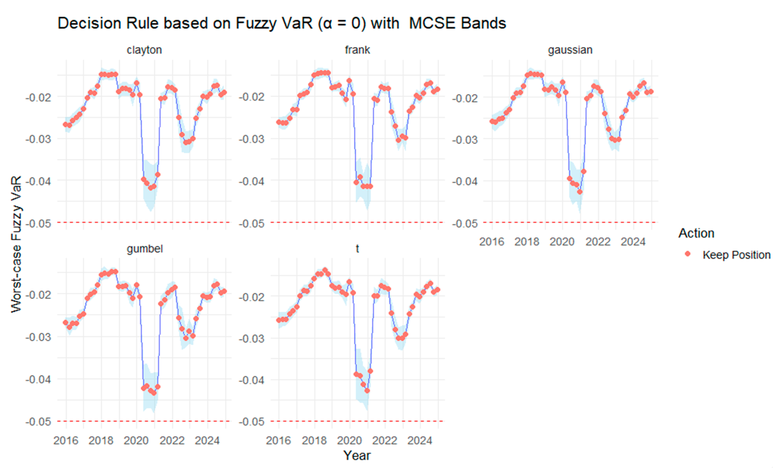
Figure 23 and

Table 8. Decision Summary Based on Fuzzy VaR (α = 0, Threshold = −5%) for the Gold–Oil Portfolio.

Family	First Date	Last Date	Worst VaR	Best VaR	Times Adjust	Times Derisk	Times Keep
Clayton	29 December 2015	11 December 2024	−0.0409	−0.0147	0	0	46
Frank	29 December 2015	11 December 2024	−0.0411	−0.0144	0	0	46
Gaussian	29 December 2015	11 December 2024	−0.0411	−0.0144	0	0	46
Gumbel	29 December 2015	11 December 2024	−0.0408	−0.0148	0	0	46
t	29 December 2015	11 December 2024	−0.0409	−0.0138	0	0	46

jointly present the time-varying fuzzy VaR outcomes for the Gold–Oil portfolio at the 95% confidence level across different copula families, with a common decision threshold of −5%. The rolling fuzzy VaR dynamics in Figure 23 capture how portfolio downside risk evolved between 1 January 2015 and 1 January 2025. The red dashed line denotes the decision threshold (−5%), indicating the boundary between acceptable and critical risk levels. Points above the line correspond to the “Keep Position” action, while values falling below it would imply risk levels exceeding the tolerance threshold. All copulas exhibit similar cyclical patterns, with noticeable risk intensifications around 2018, 2020, and 2022, periods associated with heightened commodity price volatility. These episodes are followed by rapid recoveries, reflecting the portfolio’s resilience and the time-dependent nature of dependence between gold and oil.

The shaded regions in Figure 23 represent MCSE bands scaled for visibility, confirming that simulation variability is minimal relative to fuzzy uncertainty. The curves remain consistently above the −5% threshold, indicating that the portfolio rarely enters a high-risk regime requiring de-risking or weight adjustment.

Table 8 complements these observations by summarizing the decision statistics derived from the rolling analysis. For all copula families, the number of “Adjust” and “De-risk” actions is zero, while “Keep Position” dominates (46 occurrences). This suggests that, under the specified fuzzy VaR framework, the Gold–Oil portfolio maintained stable exposure throughout the observation period. The Gaussian copula records the most conservative worst-case VaR (−0.0411), consistent with its broader tail coverage, while the Clayton and t copulas yield slightly higher best-case VaR values, implying smoother risk profiles.

Figure 24 and

Table 9. Decision Summary Based on Fuzzy CVaR (α = 0, Threshold = −5%) for the Gold–Oil Portfolio.

Family	First Date	Last Date	Worst CVaR	Best CVaR	Times Adjust	Times Derisk	Times Keep
Clayton	29 December 2015	11 December 2024	−0.1598	−0.0197	5	0	41
Frank	29 December 2015	11 December 2024	−0.0871	−0.0182	5	0	41
Gaussian	29 December 2015	11 December 2024	−0.1837	−0.0185	5	0	41
Gumbel	29 December 2015	11 December 2024	−0.1853	−0.1911	5	0	41
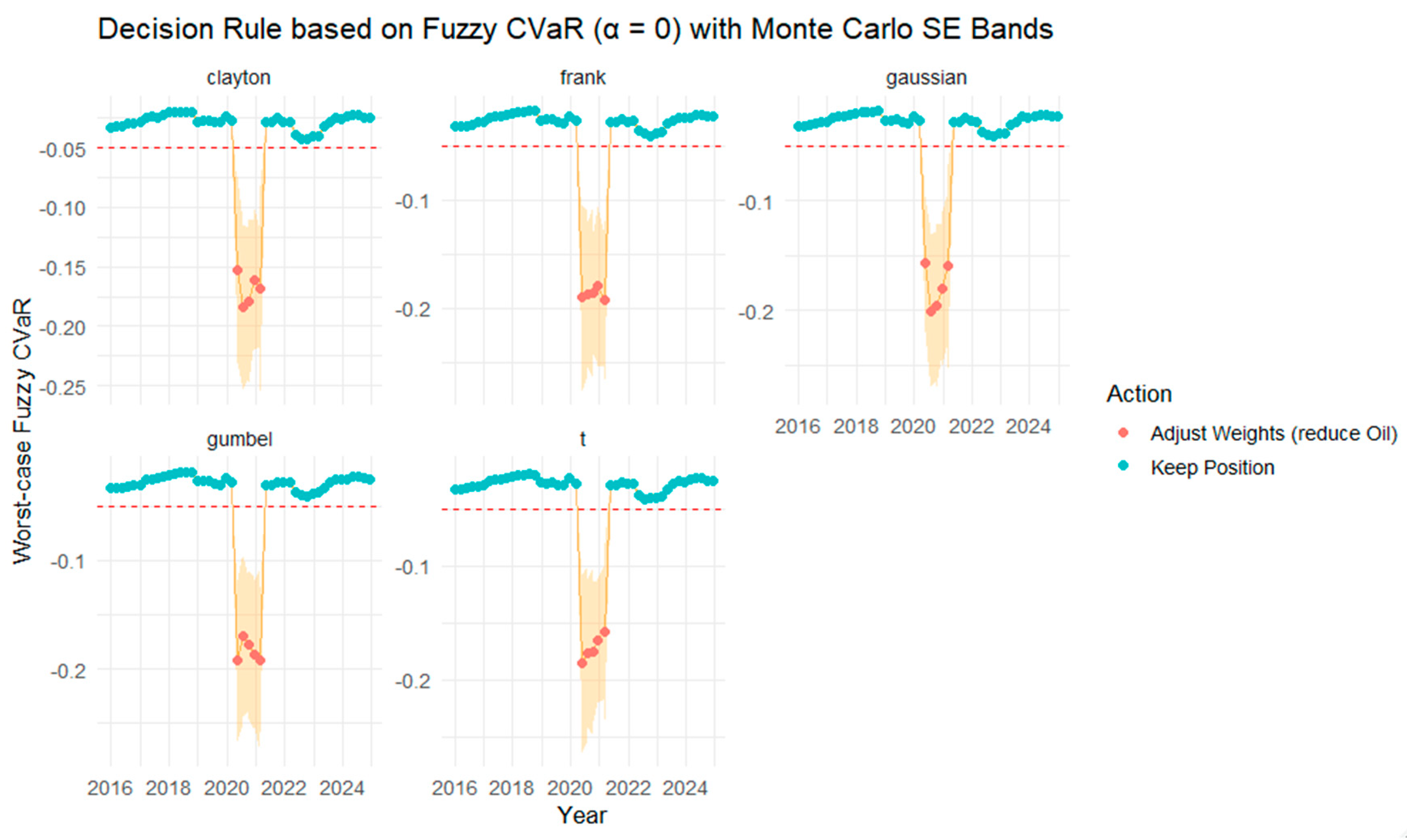
t	29 December 2015	11 December 2024	−0.1818	−0.0182	5	0	41

together illustrate the dynamic behavior of the fuzzy CVaR for the Gold–Oil portfolio under different copula families, evaluated at the 95% confidence level with α = 0 and a −5% decision threshold. The red dashed line denotes the decision threshold (−5%), marking the boundary between acceptable and critical tail-risk levels. Points above the line correspond to a “Keep Position” strategy, while points below indicate an “Adjust Weights” action (reduce Oil exposure). While fuzzy VaR identifies the loss boundary, fuzzy CVaR extends this analysis by capturing the expected losses beyond that boundary, offering a deeper assessment of tail risk. The rolling patterns in Figure 24 reveal short-lived but pronounced downward spikes, around 2020 and 2022, corresponding to periods of extreme oil price volatility and global uncertainty. These episodes triggered “Adjust Weights” decisions (marked in red), primarily under the Gaussian, Gumbel, and Clayton copulas, reflecting their sensitivity to extreme tail co-movements.

The shaded regions in Figure 24 represent MCSE bands scaled for visibility, showing that the simulation uncertainty remains relatively small compared with the magnitude of the estimated fuzzy CVaR. This confirms the numerical stability of the fuzzy tail risk estimates across rolling windows.

Table 9 complements these observations by quantifying the decision outcomes. Each copula family registered five adjustment instances, indicating consistent but limited episodes requiring portfolio rebalancing. The Gaussian copula produced the most conservative worst-case CVaR (around −0.18), capturing the strongest potential downside, whereas the Frank copula yielded the mildest risk estimate (−0.0871). Across all families, “Keep Position” remains the dominant decision (41 occurrences), confirming overall portfolio resilience in the fuzzy CVaR framework.

The fuzzy–copula VaR model, recalibrated at the 90% confidence level (α = 0.5), achieved an average exceedance rate of 8.89% across all copula families, which is consistent with the nominal 10% target. The Kupiec, Christoffersen, and conditional coverage tests yielded high p-values (approximately 0.8–1.0), confirming correct unconditional and conditional coverage as well as the independence of violations. These findings indicate that the recalibrated fuzzy–copula framework provides statistically adequate and stable VaR forecasts for the Gold–Oil portfolio, regardless of the copula specification employed.

To assess the predictive accuracy of VaR and CVaR models, an out-of-sample test was conducted using a holdout period from 1 January 2025 to 30 June 2025, with a rolling one-step-ahead approach. The results showed that the exceedance percentages for VaR and CVaR at the 1% confidence level were 0.82%, indicating that the models provided a conservative estimate of risk during the tested period.

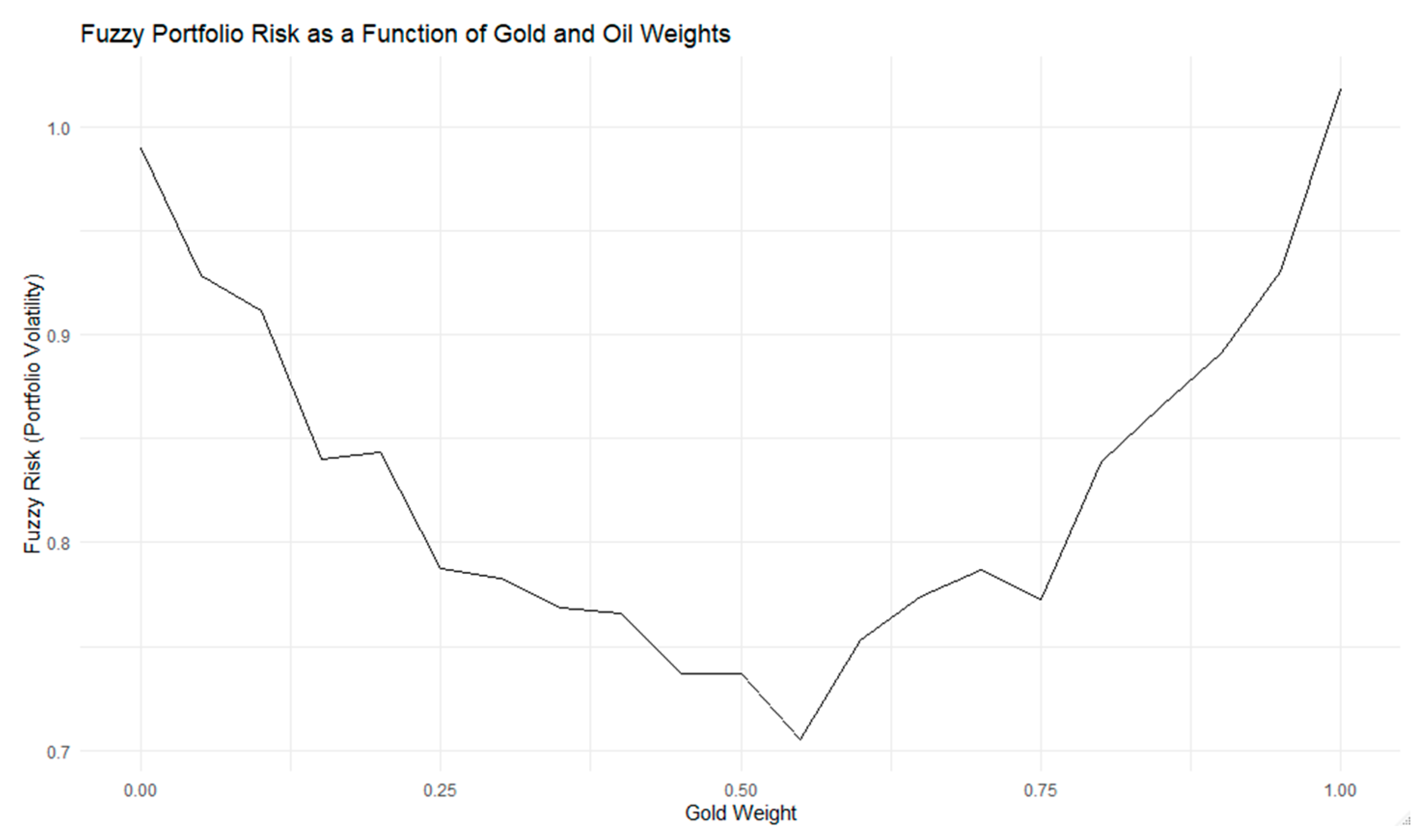
In Figure 25, the Gaussian copula is fitted to the transformed uniform margins of the Gold and Oil returns. The copula then allows for the simulation of joint returns based on the estimated dependence structure, enabling the calculation of portfolio risk by varying asset weights (Gold vs. Oil). The fuzzy risk is computed using these simulated joint returns, reflecting the uncertainty and volatility of the portfolio’s performance under different weight combinations of the two assets. The sensitivity of the portfolio’s risk to the weight allocation is particularly obvious, as the risk exhibits a non-linear relationship with the weight of Gold. This suggests that certain weight combinations, particularly those with higher or lower Gold allocations, lead to more significant changes in the overall portfolio volatility. This sensitivity highlights the importance of optimal weight allocation in managing the risk of a multi-asset portfolio, where the copula framework provides a flexible tool to capture complex dependencies between assets like Gold and Oil.

7. Conclusions

This study applied a fuzzy copula-based framework to model the dependence and tail risk of the Gold–Oil portfolio between 1 January 2015 and 1 January 2025. By introducing fuzziness into copula parameters, the model accounted for both stochastic variability and epistemic uncertainty, producing more robust VaR and CVaR estimates. The results indicated weak but asymmetric dependence between gold and oil, with Clayton and Gumbel copulas capturing stronger tail linkages. Fuzzy CVaR proved more sensitive to extreme co-movements than fuzzy VaR, especially during turbulent periods such as 2020–2021, emphasizing its usefulness for conservative risk management.

Despite its advantages, the approach has several limitations. First, it focuses on a bivariate framework, which may overlook higher-dimensional dependencies present in diversified portfolios. Second, the fuzzification of parameters relies on heuristic scaling factors that could be optimized through data-driven or Bayesian-fuzzy methods. Finally, rolling-window results depend on fixed window lengths, which may not fully capture abrupt structural shifts.

Even if the present study focuses on bivariate copulas, the proposed fuzzy optimization framework is, in principle, extendable to high-dimensional dependence modeling through vine copulas (pair-copula constructions). In such an extension, each pair-copula in the vine structure could be fuzzified using trapezoidal fuzzy parameters, allowing epistemic uncertainty to propagate across conditional dependence layers.

Future research could extend this framework to multivariate settings, explore adaptive or time-varying fuzzy copulas, and integrate machine learning or Bayesian updating to refine parameter uncertainty. Combining fuzzy dependence modeling with entropy-based or complexity measures could also enhance early-warning capabilities in financial systems.