Time-Varying Current Estimation Method for SINS/DVL Integrated Navigation Based on Augmented Observation Algorithm

Abstract

To address the problem of the bottom velocity being directly affected by the time-varying ocean currents when DVL operates in the water observation mode, it cannot be directly used for combined SINS/DVL navigation. Existing methods generally approximate small-scale, short-term currents as constant; however, this assumption is inconsistent with reality over longer durations. When the conventional Kalman filter (KF) algorithm incorporates currents into the state vector, their velocities become entangled with the SINS errors, limiting estimation accuracy. This paper proposes an augmented observation algorithm (AOA) that achieves error decoupling by enhancing DVL observation and deriving the observable current velocity equation without needing external observation information. This approach effectively estimates time-varying currents. The results from simulations and shipboard tests show that, compared to the reference algorithm (Augmented Observation Quantity Filtering algorithm (AOQ)), the proposed AOA significantly decreases the root mean square error (RMSE) of time-varying current velocity estimation by more than 67%. Additionally, the RMSE of the positioning accuracy of the combined SINS/DVL navigation is improved by over 68%.

1. Introduction

With the increasing demand for ocean exploration, resource development, and underwater reconnaissance, the importance of underwater vehicles is continuously rising, placing higher demands on the accuracy and stability of their navigation systems [1,2,3]. Due to the special electromagnetic shielding environment underwater, the Global Navigation Satellite System (GNSS) is challenging to apply effectively [4,5]. With its advantages of substantial autonomy, high concealment, and high information update rate, the SINS has become a widely adopted core navigation method for various underwater vehicles [6,7]. However, SINS’s inherent error accumulation characteristic causes its navigation accuracy to degrade over time. Simultaneously, in complex underwater environments, a single device’s navigation and positioning accuracy is challenging to meet the long-endurance, high-precision navigation requirements of underwater vehicles. Therefore, SINS must usually form an integrated navigation system with auxiliary navigation equipment [8]. Among various auxiliary devices, the DVL, which utilizes the Doppler effect for velocity measurement, provides high-precision bottom-track velocity information that can effectively suppress the position error accumulation of the SINS [9,10].

Existing DVLs typically operate in two modes: water-track mode and bottom-track mode. When the distance between the submersible and the seabed falls within the effective working range of the DVL, the bottom-track mode provides precise forward and lateral ground-referenced velocity. However, when the distance exceeds the DVL’s maximum working range or in complex environments, the DVL must switch to water-track mode, where its output reflects the velocity relative to a specific water layer. In this mode, if the ocean current velocity of that water layer is known, adding it to the DVL observation yields the submersible’s ground-referenced velocity. Therefore, when building a high-precision navigation and positioning system for underwater submersibles, it is crucial to consider the influence of ocean current velocity [11,12]. Particularly under extreme conditions, for submersibles with low speed, the ocean current velocity may surpass their speed [13]. This indicates that when the DVL operates in water-track mode, the ocean current velocity significantly affects the positioning accuracy of the SINS/DVL integrated navigation system [14,15,16].The coupling between SINS velocity error and varying ocean current velocity indicates the destruction of the symmetry of the ideal observation model, thus highlighting the necessity of using advanced estimation methods for time-varying ocean current velocity estimation.

Scholars have conducted numerous studies to reduce the impact of ocean current velocity on SINS/DVL integrated navigation accuracy. Most current studies on ocean current estimation rely on external observational data [17,18] or the prior assumption that current velocity remains constant within a given area [19]. Morgado et al., 2011 [20] proposed a Globally Asymptotically Stable (GAS) filter for position and velocity estimation based on an Ultra-Short Baseline (USBL) acoustic array system and DVL measurements, achieving performance comparable to that of the Extended Kalman Filter (EKF). However, this method heavily relies on pre-deployed large-scale acoustic arrays, resulting in high engineering costs and limited applicability. Liu et al., 2012 [21] introduced acceleration observation information based on the “current” statistical model of maneuvering targets and utilized a KF algorithm with adaptive acceleration mean and variance to estimate linear motion parameters and correct current velocity. However, this method did not address the issue of current velocity correction during DVL mode switching (water/bottom track). Batista P. et al., 2012 [22] modeled ocean current velocity as a constant and incorporated it into the state vector, using position information from a Long Baseline (LBL)/USBL combined acoustic positioning system and DVL measurements to achieve ocean current estimation via steady-state KF. Kim J. et al., 2014 [23] leveraged prior knowledge of average ocean currents in the operating sea area to reduce navigation errors for underwater gliders. Allotta, B. et al., 2017 [24] suggested augmenting the state of an Unscented Kalman Filter (UKF) to estimate the direction and magnitude of unknown ocean currents. Meurer et al., 2020 [18] employed a low-cost, lightweight, and energy-efficient sensor (DPSSv2) to estimate the 2D flow-relative velocity based on the differential pressure principle. Ben et al., 2021 [25] derived a dual-state filtering equation based on state recursion relations for estimating ocean current velocity in unknown sea areas, also assuming constant ocean current velocity within the filtering period. Compared to conventional KF, this method presents drawbacks in higher computational complexity and limited attitude observability. Huang et al., 2023 [26,27] proposed two methods based on Virtual Measurement Filters (VMF1/VMF2) and an Augmented Observation Quantity (AOQ) algorithm for estimating ocean current velocity. These methods also rely on the assumption of constant ocean current velocity within a localized range. Xie et al., 2024 [28] proposed an algorithm that dynamically optimizes the KF observation equation and measurement matrix based on the DVL operating mode (water or bottom track), effectively suppressing DVL velocity errors caused by ocean currents. However, this method still depends on the assumption of a short-term, constant ocean current. The main contributions of this manuscript are summarized below:

(1)

Unlike existing ocean current estimation methods that approximate small-scale, short-term currents as constant, we model current velocity as a first-order Markov time-varying process that better aligns with the dynamic laws of currents.

(2)

Driven by practical application needs, we propose a novel augmented observation algorithm that achieves decoupling between SINS velocity errors and time-varying currents in the observation equation for current velocity estimation.

(3)

Without requiring additional external observational data, we estimate time-varying currents within a specific horizontal motion range by constructing a new augmented observation equation and modifying the DVL observation mode.

Synthesizing existing research, the practical estimation of ocean current velocity typically relies on introducing external observational data or assumes it to be constant within short-term local ranges. This paper focuses on the problem of estimating ocean current velocity under varying conditions. The subsequent content is organized as follows: Section 2 models and analyzes the SINS/DVL integrated navigation system under the influence of currents; Section 3 constructs the observation model for the varying ocean current velocity estimation algorithm; Section 4 verifies the performance advantages of the proposed algorithm through simulation. Section 5 verifies the performance advantages of the proposed algorithm through the shipborne test. Section 6 summarizes the entire paper and discusses the results.

2. SINS/DVL Integrated Navigation System Affected by Ocean Current Influence

The definition of a coordinate system is essential to navigation research. The coordinate system utilized in this paper is illustrated in Figure 1.

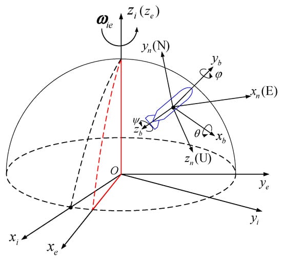
Figure 1. Schematic diagram of the coordinate system.

(1)

$i$-frame: Inertial coordinate system.

(2)

$e$-frame: Earth coordinate system.

(3)

$n$-frame: Navigation coordinate system, usually the local geographic coordinate system.

(4)

$b$-frame: An orthogonal coordinate system securely fixed to the vehicle, oriented in the right-forward-up (R-F-U) directions of the vehicle.

(5)

$d$-frame: DVL installation coordinate system ideally coinciding with the b-frame.

In this paper, it is assumed that the SINS attitude error angle is a slight angle to satisfy the approximate relationship $\sin \theta \approx \theta$, $\cos \theta \approx 1$ (where $\theta$ represents the error angle) and ignoring the earth’s gravity field model error and plumb line deviation and device installation error and scale factor error has been compensated by calibration based on the derivation of the second-order and above the neglect of a small amount of the linearization of SINS error equations can be obtained as follows:

(1) Velocity Error Equation

$$\delta {\dot{v}}^n=-{\mathit{\alpha }}^n\times {\mathit{f}}^n+\delta {\mathit{v}}^n\times \left(2{\mathit{\omega }}_{ie}^n+{\mathit{\omega }}_{en}^n\right)+{\mathit{v}}^n\times \left(2\delta {\mathit{\omega }}_{ie}^n+\delta {\mathit{\omega }}_{en}^n\right)+{\nabla }^n$$

(1)

(2) Position Error Equations

$$\delta \dot{L}={\displaystyle \frac{\delta V_N}{R_n+h}}-{\displaystyle \frac{V_N}{{\left(R_n+h\right)}^2}}\delta h$$

(2)

$$\delta \dot{\lambda }={\displaystyle \frac{\sec L}{R_e+h}}\delta V_E+{\displaystyle \frac{v_E\sec L\tan L}{R_e+h}}\delta L-{\displaystyle \frac{v_E\sec L}{{\left(R_e+h\right)}^2}}\delta h$$

(3)

(3) Attitude Error Equation

$${\dot{\mathit{\alpha }}}^n={\mathit{\alpha }}^n\times {\mathit{\omega }}_{in}^n+\delta {\mathit{\omega }}_{in}^n-{\mathit{\epsilon }}^n$$

(4)

where $\delta {\mathit{v}}^n$ is the velocity error in the navigation frame ($n$-frame), $\delta L$ is latitude error, $\delta \lambda$ is longitude error, ${\mathit{f}}^n$ is the specific force output by the accelerometers expressed in the $n$-frame, ${\nabla }^n$ is the projection of accelerometer bias in the $n$-frame, ${\mathit{\alpha }}^n$ is the attitude error angle vector, ${\mathit{\epsilon }}^n$ is the projection of gyro drift in the $n$-frame, and L is the vehicle’s local latitude.

The DVL, as an acoustic velocity sensor, measures the velocity of the vehicle relative to the seabed or a specific water layer [29]. Its measurement model in water-track mode is as follows:

$$V_{DVL}^b=C_n^b{V}_{DVL}^n+W_v=C_n^b(V^n-V_C^n)+W_v$$

(5)

where $V_{DVL}^b$ represents the DVL velocity output, $W_v$ is DVL measurement noise, $V^n$ represents the vehicle’s velocity in the $n$-frame, and $V_C^n$ is the ocean current velocity in the $n$-frame. Extensive research indicates that in stable underwater environments, ocean current velocity exhibits gradual stability characteristics over short periods and small spatial ranges. Based on this, this paper assumes that ocean current velocity follows a first-order Markov process over short-term local ranges, with its differential equation:

$${\dot{V}}_C=-\beta \cdot V_C+{\omega }_c$$

(6)

where $\beta$ is the reciprocal of the time constant, characterizing the slow-varying nature of ocean current velocity. A smaller $\beta$ value indicates a slower change in currents. ${\omega }_c$ is the driving noise, usually assumed to be Gaussian white noise.

This paper addresses the issue of estimating time-varying ocean current velocity. Consequently, it is assumed that DVL scale factor errors, misalignment errors, and lever arm errors between SINS and DVL have been corrected through pre-calibration. By neglecting the influence of the vertical channel, the eastward and northward ocean current velocity components $V_{C_E}^n$ and $V_{C_N}^n$ in the navigation frame ($n$-frame) are integrated into the subsystem state vector. Based on this, the error state equation of the SINS/DVL integrated navigation system can be derived as follows:

$$\left\{\begin{array}{l}\stackrel{.}{X}(t)=F(t)X(t)+B(t)w(t)\\ F=\left[\begin{array}{cc}{F}_{SINS}& 0\\ 0& F_{DVL}\end{array}\right]\\ X={\left[\begin{array}{cc}{X}_{SINS}^T& X_{DVL}^T\end{array}\right]}^T\end{array}\right.$$

(7)

where $X_{SINS}^T=[\Phi \hspace{1em}\delta V_{SINS}^n\hspace{1em}\delta P^n\hspace{1em}{\epsilon }_g^b\hspace{1em}{\nabla }_a^b]$, and the subsystem state transition matrix block $F_{SINS}$ is derived based on the SINS error equations. Also, $X_{DVL}={[\begin{array}{cc}{V}_{C_E}^n& V_{C_N}^n\end{array}]}^T$. According to the setting that the ocean current velocity conforms to a first-order Markov process, the elements in the sub-block $F_{DVL}$ are

$$F_{DVL}=\left[\begin{array}{cc}{e}^{-\beta \cdot \Delta t}\cdot I& 0\\ 0& e^{-\beta \cdot \Delta t}\cdot I\end{array}\right]$$

(8)

where $\beta$ is the reciprocal of the time constant, which characterizes the slow-varying nature of the current velocity; $\Delta t$ is the discrete time step.

3. Estimating Varying Currents with the Augmented Observation Algorithm (AOA)

Theoretically, the calculated navigation frame n and the ideal navigation frame n coincide. However, there is a small misalignment angle $\varphi$, so the relationship between the two coordinate systems is $C_{n^{\prime }}^n=I+\Phi \times$. The projection of the DVL measured velocity in the navigation frame ($n$-frame) is $V_{DVL}^n=C_b^n{V}_{DVL}^b$. Due to the misalignment angle, the DVL velocity in the $n^{\prime }$-frame can be obtained through coordinate transformation:

$$V_{DVL}^{n^{\prime }}=C_n^{n^{\prime }}{V}_{DVL}^n=[I-(\Phi \times )]C_b^n{V}_{DVL}^b$$

(9)

Using the updated SINS velocity and the DVL velocity differential in the $n^{\prime }$-frame for observation, we obtain:

$$\begin{array}{cc}{\tilde{V}}_{SINS}^n-V_{DVL}^{n^{\prime }}& =(V_{SINS}^n+\delta V_{SINS}^n)-[I-(\Phi \times )]C_b^n{V}_{DVL}^b\hfill \\ & =(V_{SINS}^n+\delta V_{SINS}^n)-C_b^n{V}_{DVL}^b+(\Phi \times )C_b^n{V}_{DVL}^b\hfill \\ & =(V_{SINS}^n+\delta V_{SINS}^n)-V^n+V_C^n-(C_b^n{V}_{DVL}^b)\times \Phi \hfill \\ & \approx \delta V_{SINS}^n+V_C^n-({\widehat{C}}_b^n{V}_{DVL}^b)\times \Phi \hfill \end{array}$$

(10)

where $\delta V_{SINS}^n$ denotes the velocity error of the SINS, and ${\widehat{C}}_b^n$ signifies the corrected attitude matrix. The calculation method is provided below:

$${\widehat{C}}_b^n=C_{n^{\prime }}^n{C}_b^{n^{\prime }}=(I+\Phi \times )C_b^{n^{\prime }}$$

(11)

As shown in Equation (10), the observation equation for the difference between the current SINS velocity and the DVL velocity in the $n^{\prime }$-frame includes not only the SINS velocity error $\delta V_{SINS}^n$ but also the ocean current velocity $V_C^n$. This indicates a coupling between these two quantities. Since conventional KF algorithms cannot decouple them, it is essential to establish a new measurement equation.

$${\widehat{V}}_{SINS}^n(t_{k-1})={\tilde{V}}_{SINS}^n(t_{k-1})-\delta {\widehat{V}}_{SINS}^n(t_{k-1})$$

(12)

After obtaining the actual velocity of SINS at the moment $t_{k-1}$, the carrier’s velocity at the moment $t_k$ is calculated by adding it to the velocity increment $\Delta V^n$ during the time interval $[t_{k-1},t_k]$. Considering the time-varying nature of the current velocity, the velocity increment $\Delta V^n$ during this interval can be approximated as the sum of the velocity increment $\Delta {\widehat{V}}_{DVL}^n$ and the current velocity increment $\Delta V_C^n$ output by the DVL within the navigation system $n$-frame:

$$\Delta V^n\approx \Delta {\widehat{V}}_{DVL}^n+\Delta V_C^n$$

(13)

The velocity increment of the DVL at time $t_k$, denoted as $\Delta {\widehat{V}}_{DVL}^n$, can be expressed as $V_{DVL}^n\left(t_k\right)-V_{DVL}^n\left(t_{k-1}\right)$, while the ocean current velocity increment $\Delta V_C^n$ is given by $V_C^n\left(t_k\right)-V_C^n\left(t_{k-1}\right)$. Therefore, the true velocity of the vehicle at time $t_k$ can be represented as ${\widehat{V}}_{SINS}^n\left(t_{k-1}\right)+\Delta V^n$.

The time-varying ocean current velocity observation equation can therefore be formulated as the difference between the true velocity of the vehicle at time $t_k$ and the DVL velocity $V_{DVL}^n\left(t_k\right)$.

$$\begin{array}{l}{\widehat{V}}_{SINS}^n(t_{k-1})+\Delta V^n-V_{DVL}^{n^{\prime }}(t_k)\\ =({\tilde{V}}_{SINS}^n(t_{k-1})-\delta {\widehat{V}}_{SINS}^n(t_{k-1})+V_{DVL}^{n^{\prime }}(t_k)-V_{DVL}^{n^{\prime }}(t_{k-1})+V_C^n(t_k)-V_C^n(t_{k-1}))-V_{DVL}^{n^{\prime }}(t_k)\\ \approx V^n(t_k)-(V^n(t_k)-V_C^n(t_k))\\ =V_C^n(t_k)\end{array}$$

(14)

The observation vector of the system is constructed by selecting the velocity difference between SINS and DVL in the n-frame, along with the newly established eastward and northward ocean current velocities.

$$\begin{array}{c}Z=\left[\begin{array}{l}{\tilde{V}}_{SIN{S}_E}^n(t_k)-V_{DV{L}_E}^{n^{\prime }}(t_k)\\ {\tilde{V}}_{SIN{S}_N}^n(t_k)-V_{DV{L}_N}^{n^{\prime }}(t_k)\\ {\tilde{V}}_{SIN{S}_E}^n(t_{k-1})-\delta {\widehat{V}}_{SIN{S}_E}^n(t_{k-1})-V_{DV{L}_E}^{n^{\prime }}(t_{k-1})+(e^{-\beta ·\Delta t}-1)\cdot V_{C_E}^n(t_{k-1})\\ {\tilde{V}}_{SIN{S}_N}^n(t_{k-1})-\delta {\widehat{V}}_{SIN{S}_N}^n(t_{k-1})-V_{DV{L}_N}^{n^{\prime }}(t_{k-1})+(e^{-\beta ·\Delta t}-1)\cdot V_{C_N}^n(t_{k-1})\end{array}\right]\hfill \\ \hspace{1em}=\left[\begin{array}{c}{\widehat{C}}_{3\mathrm{j}}{V}_{DVL}^b(t_k){\varphi }_N-{\widehat{C}}_{2\mathrm{j}}{V}_{DVL}^b(t_k){\varphi }_U+\delta V_{SIN{S}_E}^n(t_k)+V_{C_E}^n(t_k)\\ {\widehat{C}}_{1\mathrm{j}}{V}_{DVL}^b(t_k){\varphi }_U-{\widehat{C}}_{3\mathrm{j}}{V}_{DVL}^b(t_k){\varphi }_E+\delta V_{SIN{S}_N}^n(t_k)+V_{C_N}^n(t_k)\\ V_{C_E}^n(t_k)\\ V_{C_N}^n(t_k)\end{array}\right]\hfill \end{array}$$

(15)

where ${\widehat{C}}_{ij}$ denotes the line $i$ of ${\widehat{C}}_b^n$. The observation model is expressed in the following form:

$$Z=HX+\Theta$$

(16)

where $\Theta$ denotes the measurement noise. The measurement matrix $H$ can be obtained:

$$H=\left[\begin{array}{ccc}\begin{array}{c}0\\ -{\widehat{C}}_{3\mathrm{j}}{V}_{DVL}^b\\ 0\\ 0\end{array}& \begin{array}{c}{\widehat{C}}_{3\mathrm{j}}{V}_{DVL}^b\\ 0\\ 0\\ 0\end{array}& \begin{array}{c}-{\widehat{C}}_{2\mathrm{j}}{V}_{DVL}^b\\ {\widehat{C}}_{1\mathrm{j}}{V}_{DVL}^b\\ 0\\ 0\end{array}\end{array}\left|\begin{array}{cc}\begin{array}{c}1\\ 0\\ 0\\ 0\end{array}& \begin{array}{c}0\\ 1\\ 0\\ 0\end{array}\end{array}\left|0_{4\times 8}\left|\begin{array}{cc}\begin{array}{c}1\\ 0\\ 1\\ 0\end{array}& \begin{array}{c}0\\ 1\\ 0\\ 1\end{array}\end{array}\right.\right.\right.\right]$$

(17)

Analyzing the measurement matrix, we can see that the SINS velocity error $\delta V_{SINS}^n$ and the current velocity $V_C^n$ share the same coefficients in the first two rows, indicating a strong coupling between them. By incorporating the virtual velocity observations (corresponding to the eastward and northward velocities of the time-varying currents) in the last two rows of the measurement matrix, we can achieve decoupling between the current velocity and the SINS velocity error. Additionally, effectively estimating the time-varying current velocities can be accomplished by introducing the DVL bottom observations at the right time.

4. Simulation Tests

4.1. Simulation Test Setup

To verify the performance of the proposed broadening observation algorithm in estimating the velocity of changing currents under the DVL water-to-bottom spacing observation scenario, simulation tests have been conducted. Combined with the underwater vehicle’s use case, the vehicle’s depth can be accurately obtained using the depth gauge; therefore, the vehicle’s depth and celestial velocity will not be considered in the simulation test. The actual navigation trajectory in the simulation test is shown in Figure 2. At the same time, the attitude and velocity information is displayed in Figure 3. The simulation conditions are as follows: the initial attitude is set to $[0^{°}{ 0}^{°}{ 30}^{°}]$, the initial velocity is 0, the initial position is set to $[{30}^{°}{ 124}^{°}{-50}^{°}]$, and the vehicle accelerates to 5 m/s with an acceleration of 1 m/s² before moving at a constant speed of 5 m/s. The entire simulation process takes approximately 4200 s.

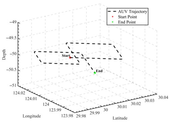
Figure 2. The trajectory of AUV simulation test.

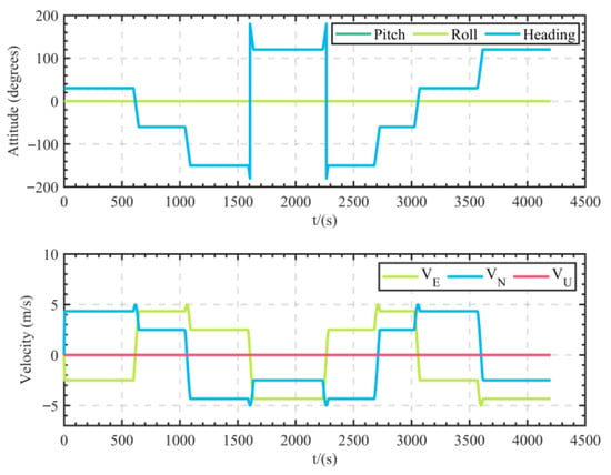
Figure 3. Attitude and velocity information of AUV simulation test.

To validate the usability and effectiveness of the algorithm, it is essential to generate ideal angular velocity and acceleration information based on the trajectory using the SINS guidance inversion algorithm, which utilizes data from SINS and DVL. According to the inertial sensor specifications and the errors of DVL in Table 1, the output from the inertial measurement unit (IMU) can be obtained by superimposing the bias and random error information on the ideal values. Assuming that the current velocity conforms to a first-order Markov process and considering the environment in which the navigator is used, the initial velocities of the eastward and northward currents are set to [0.5, 0.8] m/s. The velocities are shown in Figure 4. The DVL operates in a mode with intervals of water-to-water and bottom-to-bottom observations, including water-to-water observation phases from 1 s to 1030 s; simultaneous water-to-water and bottom-to-bottom observation phases from 1031 s to 2230 s, and simultaneous water-to-bottom observation phases from 2231 s to 4200 s. The DVL output provides the velocity information under the carrier system. The DVL velocity information under the constructed navigation system is illustrated in Figure 5, assuming that the scale factor, installation error, and other errors of the DVL have been properly calibrated.

Table 1. The specifications of the inertial sensors and DVL error setting.

Items	Index	Values
Gyro	Bias	$0.003 \mathrm{deg}/\mathrm{h}$
	Angular Random Walk	$0.0005 \mathrm{deg}/\sqrt{\mathrm{h}}$
Accelerometer	Bias	$50 \mathrm{\mu }\mathrm{g}$
	Random Walk Noise	$50 \mathrm{\mu }\mathrm{g}/\sqrt{\mathrm{H}\mathrm{z}}$
DVL	Random Noise	0.3 cm/s

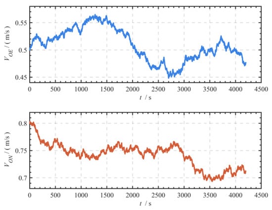
Figure 4. The simulation of eastward and northward ocean current velocities based on a first-order Markov process.

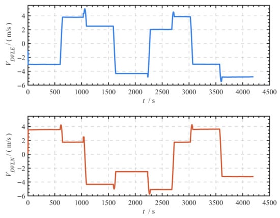
Figure 5. East and North DVL velocities.

In the combined underwater SINS/DVL navigation system, where velocity error serves as the observation quantity, there is no external information source to provide the absolute velocity and position information of the carrier. Consequently, any velocity and position errors at the initial moment will not be corrected by its algorithmic iteration in the subsequent navigation process. Therefore, during the simulation test for algorithm validation, the initial velocity and position errors are set to 0. For the validation of the algorithm, the initial iteration conditions are as follows: the initial iteration value of the error angle is set to $[{0.5}^{°} -0{.5}^{°}{ 5}^{°}]$, the velocity error is set to [0.1 0.1 0.1] m/s, the position error is set to [1 1 5] m, the accelerometer bias is set to [50 50 50] µg, and the gyroscope bias is set to [0.005 0.005 0.005] deg/h. Since the current velocity is unknown, the initial values of the eastward and northward current speeds are set to [0 0] m/s.

4.2. Simulation Test Results

To verify the performance of the proposed AOA based on time-varying current velocity estimation, the AOQ algorithm referenced in [27] is utilized to compare the current velocity estimation with that of the AOA. Additionally, the SINS/DVL velocity matching is performed based on this, and the simulation results are obtained as follows under the specified simulation conditions:

Figure 6 and Figure 7 show the comparison of estimation results for the eastward and northward current velocities, respectively. The performance difference between the AOQ method and the AOA method is a significant feature in the dynamic current environment. It is worth noting that during the joint observation phase from 1031 s to 2230 s, DVL performs water and bottom observations simultaneously. At this time, the differences between the two modes of observation can be directly resolved to obtain the high-precision baseline current velocity. The simulation results indicate that the AOA method has a better capability for estimating time-varying current velocities than the AOQ method in the single water observation mode. The RMSE of the eastward current velocity estimation is reduced by about 88.89% (RMSE 0.144 m/s → 0.016 m/s), while that of the northward current velocity estimation is reduced by about 67.74% (RMSE 0.031 m/s → 0.010 m/s).

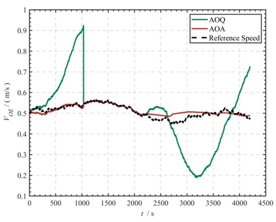
Figure 6. Comparison of eastward ocean current velocity estimations.

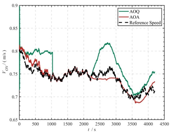
Figure 7. Comparison of northward ocean current velocity estimations.

In the simulation experiments, the estimated current velocities were used to compensate for the DVL velocities of the interval-to-bottom measurements from the above simulation, thereby obtaining the relative full DVL-to-bottom velocities. The results of SINS/DVL velocity matching using the obtained DVL-to-bottom velocities and SINS/DVL velocity matching utilizing the KF algorithm on the DVL velocities measured at the interval to the bottom without current velocity compensation serve as comparisons. The results are presented in Figure 8 and Figure 9, as well as in Table 2.

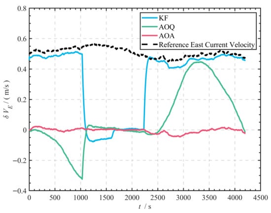
Figure 8. Comparison of eastward velocity errors among the three methods in the simulation experiment.

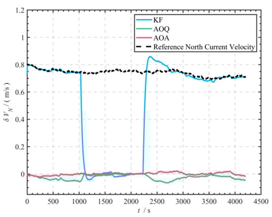
Figure 9. Comparison of northward velocity errors among the three methods in the simulation experiment.

Table 2. Statistical characteristics of eastward and northward velocity errors for the three methods.

	$\mathit{\delta }{\mathit{V}}_{\mathit{E}}$ (m/s)			$\mathit{\delta }{\mathit{V}}_{\mathit{N}}$ (m/s)
	RMSE	Mean	MAX	RMSE	Mean	MAX
KF	0.397	0.463	0.514	0.628	0.710	0.860
AOQ	0.205	0.059	0.447	0.031	0.019	0.065
AOA	0.015	0.006	0.046	0.009	0.005	0.024

The velocity errors obtained from uncompensated DVL for water observation velocity matching are highly consistent with the time-frequency characteristics of currents (correlation coefficient reaching 0.60). After compensation using the AOQ method, the RMSE of the eastward velocity errors obtained from bottom observation velocity was reduced by approximately 48.36% relative to the KF algorithm, with the mean value decreasing by approximately 87.26%, the maximum value decreased by approximately 13.03%; the RMSE of northward velocity errors decreased by approximately 95.06%, the mean decreased by approximately 97.32%, and the maximum value decreased by approximately 92.44%. Notably, the AOA method demonstrated superior convergence characteristics compared to the AOQ method, with the RMSE of eastward velocity errors reduced by approximately 92.68% relative to the AOQ algorithm, the mean decreased by approximately 89.83%, and the maximum decreased by 89.71%, the northward velocity error RMSE decreased by approximately 70.97%, the mean decreased by approximately 73.68%, and the maximum decreased by 63.08%.

Simulation test data reveal significant differences in navigation accuracy among the three algorithms (Figure 10, Figure 11 and Figure 12, Table 3). Without current compensation, the positioning error of the SINS/DVL velocity matching method (RMSE 2733.487 m) is comparable to that of the pure inertial navigation solution (RMSE 7293.011 m). The compensated methods significantly enhance navigation performance: the AOQ algorithm reduces latitude position error by approximately 95.53% (RMSE 1216.898 m → 54.409 m) and longitude error by about 80.95% (RMSE 726.014 m → 138.272 m); in comparison, the AOA algorithm achieves even greater error reduction: latitude position error is further reduced by approximately 86.37% (RMSE 54.409 m → 7.414 m) based on the AOQ algorithm, and longitude error decreases by around 91.76% (RMSE 138.272 m → 11.398 m). The box plot (Figure 11) indicates that the median of the error distribution for AOA is approximately 89.61% lower than that of AOQ (Mean 121.223 m → Mean 12.600 m), with no outliers observed. Notably, when the DVL utilized the seabed synchronous observation mode (Phase II 1031–2230 s), the position error growth rate decreased by around 96.44% compared to the continuous water-facing observation mode (from 0.900 m/s to 0.032 m/s). Position error plots and trajectory comparison diagrams (Figure 10 and Figure 12) clearly demonstrate that the average offset between the AOA solution trajectory and the actual trajectory is significantly smaller than that of the AOQ and KF algorithms, validating the usability and effectiveness of the proposed algorithm.

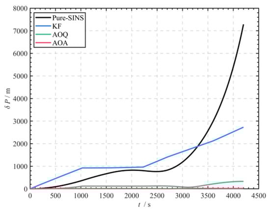
Figure 10. Comparison of position errors obtained using three methods with pure SINS.

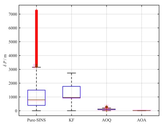
Figure 11. Box plot of position errors.

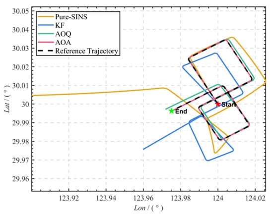
Figure 12. Trajectory comparison by using different methods in simulation test.

Table 3. Statistical characteristics of latitude and longitude errors for the three methods.

	$\mathit{\delta }{\mathit{P}}_{\mathit{L}\mathit{a}\mathit{t}}$ (m)			$\mathit{\delta }{\mathit{P}}_{\mathit{L}\mathit{o}\mathit{n}}$ (m)
	RMSE	Mean	MAX	RMSE	Mean	MAX
Pure-SINS	455.133	272.851	921.833	2050.772	584.449	7234.517
KF	1216.898	828.379	2302.654	726.014	495.239	1473.002
AOQ	54.409	37.989	96.492	138.272	115.006	317.214
AOA	7.414	7.077	10.923	11.398	6.918	20.882

5. Shipborne Experiments

5.1. Shipborne Experiments Test Setups

To validate the ability of the algorithm proposed in this paper to estimate dynamic ocean current velocities under bottom observation conditions with DVL intervals, this study conducted ship-based dynamic experiments in Lake (31.1173° N, 114.4656° E). The experimental platform integrates a navigation-grade laser-based inertial navigation system (sampling rate of 200 Hz), a multi-antenna GPS receiver (positioning accuracy of 10 cm), an RTK positioning system (update rate of 1 Hz), a DVL (operating frequency of 600 kHz), and a data acquisition workstation. The main technical parameters of the equipment are detailed in Table 4, and the system integration architecture is shown in Figure 13. The test process is divided into two phases: (1) Initial alignment phase (0–1000 s): Maintain the vessel stationary to complete the SINS initial alignment; (2) Dynamic navigation phase (selected 1200 s): Execute variable-speed maneuvers along a predefined route and generate a reference trajectory (Figure 14) using the high-precision SINS/GPS integrated navigation system (position accuracy 0.1 m) for algorithm performance evaluation.

Table 4. Specification parameters of inertial sensors, DVL and GPS.

Device Name	Parameter	Parameter Metric
CY-JG901 Laser-type SINS	Gyroscope Constant Bias	$<0.003°/\mathrm{h}$
	Gyroscope Random Bias	$<0.001°/\sqrt{\mathrm{h}}$
	Accelerometer Bias	$<50 \mathrm{\mu }\mathrm{g}$
	Accelerometer Random Noise	$<10 \mathrm{\mu }\mathrm{g}/\sqrt{\mathrm{Hz}}$
	Update Rate	200 Hz
IACAS DVL_PA600	Random Noise	$0.003 \mathrm{m}/\mathrm{s}$
	Measure Range	$-12 \mathrm{k}\mathrm{n}\mathrm{o}\mathrm{t}~12 \mathrm{k}\mathrm{n}\mathrm{o}\mathrm{t}$
	Bottom-track Depth	80 m
	Operating Rate	600 kHz
	Update Rate	1 Hz
GPS	Positioning Accuracy	$<0.1m@1\mathrm{Hz}\left(\mathrm{RTK}\right)$

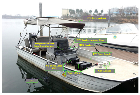
Figure 13. Experiment platform and equipment.

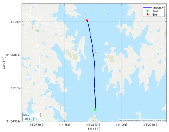
Figure 14. Ship-mounted experiment track map.

To address the physical limitations of the DVL’s continuous bottom observation mode in the measured data, this study employs numerical simulation methods to construct equivalent observation scenarios, thus validating the effectiveness of the dynamic ocean current estimation algorithm. Based on Equation (5), a DVL water observation velocity model was established, and ocean current velocities were simulated using Equation (6). Initial velocities were set to [0.5, 0.8] m/s, and the temporal characteristics of the generated ocean current velocity field are shown in Figure 15. To simulate the actual DVL operating mode, a segmented observation strategy was designed, consisting of three phases: Phase I (0–400 s), pure water observation; Phase II (401–600 s), simultaneous water and seabed observation; and Phase III (601–1200 s), pure water observation. Other experimental conditions were set similarly to the simulation experiments.

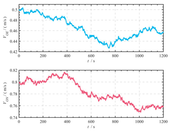
Figure 15. Eastward and northward current velocities generated by simulation.

5.2. Shipborne Experiments Results

Figure 16 and Figure 17 compares the performance differences between the AOQ and AOA algorithms in dynamic ocean current estimation. During the synchronized seafloor observation phase (Phase II: 401–600 s), the DVL directly obtains the reference ocean current velocity from the water/seabed velocity difference values. Experimental data show that during the pure water observation phase (Phase I and III), the AOA algorithm demonstrates superior time-varying ocean current velocity tracking capability compared to the AOQ algorithm, with the RMSE of eastward ocean current velocity estimates reduced by approximately 71.11% (0.045 m/s → 0.013 m/s) and the RMSE of northward ocean current velocity estimates reduced by approximately 87.67% (0.073 m/s → 0.009 m/s).

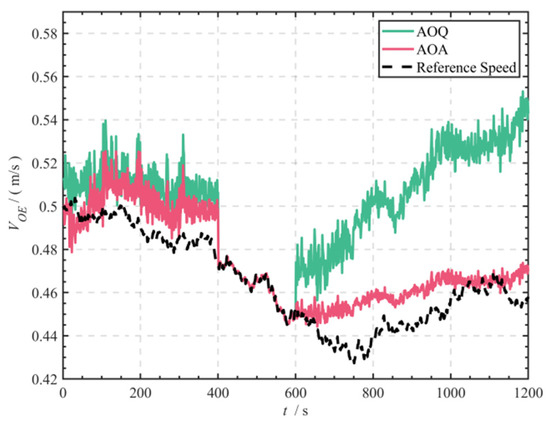
Figure 16. Comparison of eastward current velocity estimates in the Lake experiment.

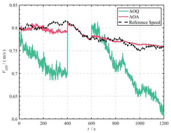
Figure 17. Comparison of northward current velocity estimates in the Lake experiment.

In the Lake experiment, the DVL velocity observations based on the method described above were initially constructed using interval bottom measurements. Two algorithms were then employed to estimate ocean current velocities, which were used for dynamic compensation to obtain relative velocities equivalent to those derived from the two algorithms and the full-time bottom observation mode. Subsequently, SINS/DVL velocity matching was conducted on the compensated DVL bottom observation velocities. To assess the effectiveness of the compensation, a comparison experimental group was established simultaneously: the DVL bottom-bearing velocity from the interval bottom-bearing measurement mode, without current compensation, was directly subjected to SINS/DVL matching using the KF algorithm.

The experimental results are presented in Figure 18 and Figure 19, as well as in Table 5. The three methods demonstrate significant differences in eastward and northward velocity errors, along with their statistical characteristics: the velocity error obtained from the uncompensated DVL in matching water observation velocities closely aligns with the time-frequency characteristics of currents (correlation coefficient reaching 0.73). Meanwhile, the RMSE of eastward velocity errors, derived from bottom-observed velocities compensated using the AOQ method, was reduced by approximately 88.47% compared to the KF algorithm. The mean value decreased by about 91.89%, and the maximum value decreased by roughly 77.88%. The RMSE of northward velocity errors was reduced by about 89.37%, with the mean value decreasing by around 91.74% and the maximum value decreasing by approximately 79.63%. Notably, the AOA method exhibited superior convergence characteristics compared to the AOQ method. The RMSE of eastward velocity errors using the AOA method was decreased by roughly 53.06% relative to the AOQ algorithm, with the mean dropping by around 59.46% and the maximum decreasing by 44%. Similarly, the RMSE of northward velocity errors was lowered by approximately 68.42%, with the mean value reduced by about 76.56% and the maximum value decreasing by 50%.

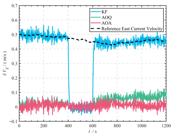
Figure 18. Comparison of eastward velocity errors among the three methods in the Lake experiment.

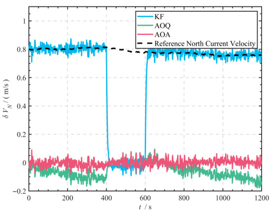
Figure 19. Comparison of northward velocity errors among the three methods in the Lake experiment.

Table 5. Statistical characteristics of eastward and northward velocity errors for the three methods in the Lake experiment.

	$\mathit{\delta }{\mathit{V}}_{\mathit{E}}$ (m/s)			$\mathit{\delta }{\mathit{V}}_{\mathit{N}}$ (m/s)
	RMSE	Mean	MAX	RMSE	Mean	MAX
KF	0.425	0.456	0.565	0.715	0.775	0.874
AOQ	0.049	0.037	0.125	0.076	0.064	0.178
AOA	0.023	0.015	0.070	0.024	0.015	0.089

The experimental data from Lake reveal significant differences in navigation accuracy among the three algorithms (Figure 20, Figure 21 and Figure 22, Table 6). Compared to the KF algorithm without current speed compensation, the methods with current speed compensation significantly enhance navigation performance: the AOQ algorithm reduces the latitude position error by approximately 91.42% (RMSE 441.174 m → 37.837 m), while the longitude error decreases by approximately 93.20% (RMSE 261.453 m → 17.771 m). In contrast, the AOA algorithm achieved even greater improvements: the latitude position error was further reduced by approximately 86.32% (RMSE 37.837 m → 5.175 m) compared to the AOQ algorithm, and the longitude error decreased by approximately 68.94% (RMSE 17.771 m → 5.520 m). Box plot analysis (Figure 21) further indicates that the median of the error distribution for AOA decreased by approximately 79.46% (Mean 35.235 m → Mean 7.238 m) compared to AOQ, with no outliers observed. It is also worth noting that when the DVL adopts the seabed synchronous observation mode (Phase II 401–600 s), the position error growth rate is reduced by approximately 98.73% compared to the continuous water-facing observation mode (from 0.948 m/s to 0.012 m/s). Position error plots and trajectory comparison diagrams (Figure 20 and Figure 22) clearly show that the average offset between the AOA solution trajectory and the actual trajectory is significantly smaller than that of the AOQ and KF algorithms, validating the usability and effectiveness of the proposed algorithm.

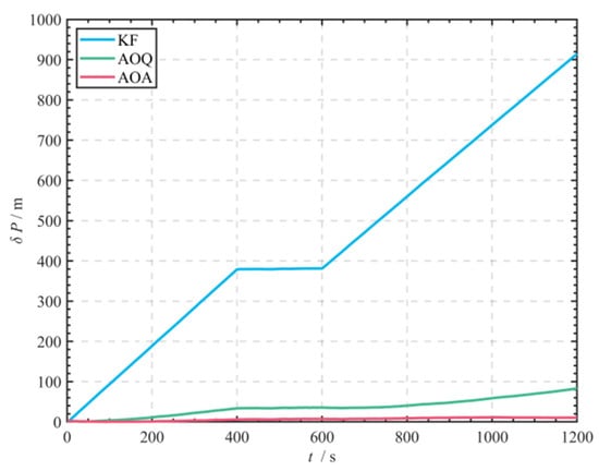
Figure 20. Comparison of position errors obtained using three methods.

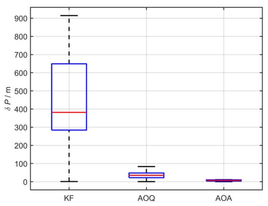
Figure 21. Box plot of position errors.

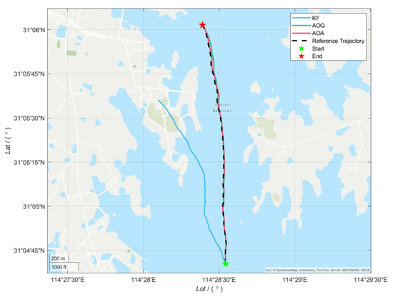
Figure 22. Trajectory comparison by using different methods in the Lake experiment.

Table 6. Statistical characteristics of latitude and longitude errors for the three methods in the Lake experiment.

	$\mathit{\delta }{\mathit{P}}_{\mathit{L}\mathit{a}\mathit{t}}$ (m)			$\mathit{\delta }{\mathit{P}}_{\mathit{L}\mathit{o}\mathit{n}}$ (m)
	RMSE	Mean	MAX	RMSE	Mean	MAX
KF	441.174	327.230	787.861	261.453	197.314	466.375
AOQ	37.837	34.248	72.310	17.771	7.503	41.769
AOA	5.175	5.547	7.594	5.520	3.902	9.521

6. Discussion and Conclusions

In deep-sea navigation scenarios, the SINS/DVL combination navigation system faces significant challenges in water observation mode. The DVL velocity, which has not been compensated for time-varying currents, directly contributes to velocity matching, exponentially increasing navigation errors. Current mainstream estimation algorithms (such as those proposed by Ben, Huang et al.) are based on the assumption of steady currents, limiting their applicability to short-term or small-scale, stable flow fields. They struggle to adjust to the non-steady flow fields common in real-world marine environments.

The Augmented Observation Algorithm (AOA) proposed in this paper enables the estimation and compensation of ocean current velocity by modifying the DVL observation mode. This allows the accurate real-time current velocity to be obtained during bottom-tracking phases through the difference between bottom-track and water-track velocities. Most current estimation algorithms assume that the current velocity remains constant within a specific range, which considerably limits underwater vehicles’ operational duration and mobility range. Adopting the proposed intermittent bottom-tracking mode allows the vehicle to maintain sustained operation over extended periods and in varying current environments within a defined accuracy range, thereby effectively enhancing its deployment duration and operational scope. Simulation and lake trial data results indicate that, compared to the traditional KF algorithm and AOQ algorithm, the AOA algorithm demonstrates superior performance in terms of estimating variable ocean current velocities, as well as reducing eastward and northward velocity errors and longitude and latitude position errors. To clearly demonstrate the key differences among the algorithms, a comparison table of KF, AOQ, and AOA is constructed as shown in Table 7:

Table 7. Core differences among the algorithms.

Item	KF (Kalman Filter)	AOQ (Augmented Observation Quantity)	AOA (Proposed Method)
Current Modeling	Not explicitly modeled	Constant assumption ${\dot{V}}_C=0$	First-order Markov process ${\dot{V}}_C=-\beta V_C+{\omega }_c$
DVL Mode	Conventional water/bottom tracking	Water-track mode	Intermittent bottom-track mode
Error Coupling	Strongly coupled, not decoupled	Decoupled	Decoupled
Current Estimation Capability	None	Suitable for constant currents	Suitable for time-varying currents
Estimation Accuracy (RMSE)	Low	Medium	High (improvement ≥ 67%)
Applicable Scenario	Short-term/small area	Local slow-varying currents	Long-endurance/dynamic current environments

While certain progress has been made in estimating time-varying ocean current velocity, it should be noted that existing current estimation algorithms still face challenges in maintaining effectiveness under sustained water-track mode. Achieving dynamic current estimation across arbitrary DVL observation modes remains an unresolved challenge, and addressing this limitation represents a key focus of our future research in ocean current estimation algorithms.

References

- Zhang, L.; Wu, S.; Tang, C. Cooperative positioning of underwater unmanned vehicle clusters based on factor graphs. Ocean Eng. 2023, 287, 115854. [Google Scholar] [CrossRef]
- Huang, H.; Tang, J.; Liu, C.; Zhang, B.; Wang, B. Variational Bayesian-based filter for inaccurate input in underwater navigation. IEEE Trans. Veh. Technol. 2021, 70, 8441–8452. [Google Scholar] [CrossRef]
- Zhang, T.; Tang, J.; Qin, S.; Wang, X. Review of navigation and positioning of deep-sea manned submersibles. J. Navig. 2019, 72, 1021–1034. [Google Scholar] [CrossRef]
- Lin, E.; Xu, J.; Zha, F.; He, H.; Wu, M. Linear track underwater carrier SINS correction method based on hydroacoustic single beacon. IEEE Access 2022, 10, 4750–4762. [Google Scholar] [CrossRef]
- Ansari-Rad, S.; Hashemi, M.; Salarieh, H. Pseudo DVL reconstruction by an evolutionary TS-fuzzy algorithm for ocean vehicles. Measurement 2019, 147, 106831. [Google Scholar] [CrossRef]
- Tang, J.; Bian, H. Ship SINS/CNS Integrated Navigation Aided by LSTM Attitude Forecast. J. Mar. Sci. Eng. 2024, 12, 387. [Google Scholar] [CrossRef]
- Dai, H.F.; Bian, H.W.; Wang, R.Y.; Ma, H. An INS/GNSS integrated navigation in GNSS denied environment using recurrent neural network. Def. Technol. 2020, 16, 334–340. [Google Scholar] [CrossRef]
- Zhang, S.; Zhang, T.; Zhang, L. An underwater SINS/DVL integrated system outlier interference suppression method based on LSTM-EEWKF. IEEE Sens. J. 2023, 23, 27590–27600. [Google Scholar] [CrossRef]
- Liu, P.; Wang, B.; Deng, Z.; Fu, M. INS/DVL/PS tightly coupled underwater navigation method with limited DVL measurements. IEEE Sens. J. 2018, 18, 2994–3002. [Google Scholar] [CrossRef]
- Liu, S.; Zhang, T.; Zhang, J.; Zhu, Y. A new coupled method of SINS/DVL integrated navigation based on improved dual adaptive factors. IEEE Trans. Instrum. Meas. 2021, 70, 1–11. [Google Scholar] [CrossRef]
- Wu, Y.; Wang, X.; Zhao, Y.; Tang, Y. Research on SINS/DVL integrated navigation algorithm affected by ocean current. In Proceedings of the AOPC 2020: Optical Sensing and Imaging Technology, Beijing, China, 30 November–2 December 2020; SPIE: Bellingham, WA, USA; Volume 11567, pp. 905–910. [Google Scholar]
- Wang, D.; Xu, X.; Yao, Y.; Zhang, T.; Zhu, Y. A novel SINS/DVL tightly integrated navigation method for complex environment. IEEE Trans. Instrum. Meas. 2019, 69, 5183–5196. [Google Scholar] [CrossRef]
- Guo, Y.S.; Fu, M.Y.; Deng, J.Q.; Deng, Z.H.; Ai, Y.T. SINS/DVL integrated navigation algorithm considering the impact of ocean currents. Zhongguo Guanxing Jishu Xuebao/J. Chin. Inert. Technol. 2017, 25, 738–742. [Google Scholar]
- Zhu, B.; He, H. Integrated navigation for Doppler velocity log aided strapdown inertial navigation system based on robust IMM algorithm. Optik 2020, 217, 164871. [Google Scholar] [CrossRef]
- Chang, G. Robust Kalman filtering based on Mahalanobis distance as outlier judging criterion. J. Geod. 2014, 88, 391–401. [Google Scholar] [CrossRef]
- Zhu, B.; Chang, L.; Xu, J.; Zha, F.; Li, J. Huber-based adaptive unscented Kalman filter with non-Gaussian measurement noise. Circuits Syst. Signal Process. 2018, 37, 3842–3861. [Google Scholar] [CrossRef]
- Hegrenaes, Ø.; Hallingstad, O. Model-aided INS with sea current estimation for robust underwater navigation. IEEE J. Ocean. Eng. 2011, 36, 316–337. [Google Scholar] [CrossRef]
- Meurer, C.; Fuentes-Pérez, J.F.; Schwarzwälder, K.; Ludvigsen, M.; Sorensen, A.J.; Kruusmaa, M. 2D estimation of velocity relative to water and tidal currents based on differential pressure for autonomous underwater vehicles. IEEE Robot. Autom. Lett. 2020, 5, 3444–3451. [Google Scholar] [CrossRef]
- Medagoda, L.; Williams, S.B.; Pizarro, O.; Kinsey, J.C.; Jakuba, M.V. Mid-water current aided localization for autonomous underwater vehicles. Auton. Robot. 2016, 40, 1207–1227. [Google Scholar] [CrossRef]
- Morgado, M.; Batista, P.; Oliveira, P.; Silvestre, C. Position USBL/DVL sensor-based navigation filter in the presence of unknown ocean currents. Automatica 2011, 47, 2604–2614. [Google Scholar] [CrossRef]
- Liu, Q.; Xu, X.S.; Xu, J.N. DVL/SIMU dead-reckoning method based on “current” statistical model. Zhongguo Guanxing Jishu Xuebao 2012, 20. [Google Scholar]
- Batista, P.; Silvestre, C.; Oliveira, P. GES integrated LBL/USBL navigation system for underwater vehicles. In Proceedings of the 2012 IEEE 51st IEEE Conference on Decision and Control (CDC), Maui, HI, USA, 10–13 December 2012; pp. 6609–6614. [Google Scholar]
- Kim, J.; Park, Y.; Lee, S.; Lee, Y.K. Underwater glider navigation error compensation using sea current data. IFAC Proc. Vol. 2014, 47, 9661–9666. [Google Scholar] [CrossRef]
- Allotta, B.; Costanzi, R.; Fanelli, F.; Monni, N.; Paolucci, L.; Ridolfi, A. Sea currents estimation during AUV navigation using Unscented Kalman Filter. IFAC-PapersOnLine 2017, 50, 13668–13673. [Google Scholar] [CrossRef]
- Ben, Y.; Zang, X.; Li, Q.; He, J. A Dual-State Filter for a Relative Velocity Aiding Strapdown Inertial Navigation System. IEEE Trans. Instrum. Meas. 2021, 70, 1–15. [Google Scholar] [CrossRef]
- Huang, Y.; Liu, X.; Shao, Q.; Wang, Z. Virtual Metrology Filter-Based Algorithms for Estimating Constant Ocean Current Velocity. Remote Sens. 2023, 15, 4097. [Google Scholar] [CrossRef]
- Huang, Y.; Liu, X.; Wang, Z.; Wu, X. Estimation of constant ocean current velocity based on SINS/DVL integrated navigation with an augmented observable quantities filter. Ocean Eng. 2023, 284, 115288. [Google Scholar] [CrossRef]
- Xie, Y.; Xiong, Z.; Ca, J.; Cai, S.; Luo, K. An Underwater SINS/DVL Integrated Navigation Method Considering Unknow and Constant Ocean Current Velocity. In Proceedings of the International Conference on Guidance, Navigation and Control, Changsha, China, 9–11 August 2024; Springer Nature: Singapore, 2024; pp. 330–340. [Google Scholar]
- Liu, P.; Wang, B.; Deng, Z.; Fu, M. A correction method for DVL measurement errors by attitude dynamics. IEEE Sens. J. 2017, 17, 4628–4638. [Google Scholar] [CrossRef]
Disclaimer/Publisher’s Note: The statements, opinions and data contained in all publications are solely those of the individual author(s) and contributor(s) and not of MDPI and/or the editor(s). MDPI and/or the editor(s) disclaim responsibility for any injury to people or property resulting from any ideas, methods, instructions or products referred to in the content. |
© 2025 by the authors. Licensee MDPI, Basel, Switzerland. This article is an open access article distributed under the terms and conditions of the Creative Commons Attribution (CC BY) license (https://creativecommons.org/licenses/by/4.0/).