Bayesian Model Averaging with Diffused Priors for Model-Based Clustering Under a Cluster Forests Architecture

Abstract

This paper considers a class of generative graphical models for parsimonious modeling of Gaussian mixtures and robust unsupervised learning, each assuming that the data are generated independently and identically from a finite mixture model with an extended naïve Bayes structure. To account for model uncertainty, the expectation model-averaging algorithm, which approximates the Bayesian model averaging with incomplete data, is introduced using a novel class of non-informative priors for the parameters. A Cluster Forests architecture to circumvent intractable model averaging over a large selective model space is developed. Extensive synthetic data experiments and real-world data applications show that the proposed methodology can produce clustering results of high robustness and attain good model detection performance.

1. Introduction

Finite Gaussian mixture models are powerful tools for modeling the distributions of random phenomena. They are widely used for unsupervised classification tasks and lay the foundation for many deep learning-based clustering algorithms [1,2]. However, the competitive performance of Gaussian mixture models cannot be expected for high-dimensional datasets due to the curse of dimensionality [3]. They are easily over-parameterized and may suffer from singularity problems when the sample size is small [4]. Moreover, the impact of redundancy and noise can degrade the model’s interpretability and efficiency, resulting in a model with limited generalization capacity [5,6].

Parsimonious modeling of Gaussian mixture models via feature selection aims to reduce the dimensions by retaining only the discriminative features for clustering. Related approaches are commonly established under the local independence assumption [7,8], i.e., adopting a diagonal component covariance matrix, which facilitates computational efficiency but damages the flexibility of modeling the dependence relationship across features. It has been shown in experiments that the local independence assumption can be easily violated in real-world datasets [9,10]. Ignorance of the correlations may undermine the reliability of classification algorithms and lead to misleading conclusions about the feature’s saliency [11]. Moreover, in addition to the prediction performance, scientists are often interested in describing the relationships between attributes as in generative models. Modeling the covariance structures can result in better data generating performance [1].

To allow for the presence of within-component dependence, Celeux and Govaert [12] proposed parsimonious models derived from spectral decomposition of the component covariance matrices. The model family related to the local factor analysis was suggested in [13,14]. Fop et al. [15] proposed to construct the mixture components directly via sparse covariance graphs. Moreover, by viewing the components as Gaussian graphical models, the graphical Lasso path of solutions for sparsity patterns was adopted in [16]. Nevertheless, these specifications are only designed for parsimonious modeling of the covariance structures and are generally not extendable for feature selection purposes.

In this paper, we consider the block-diagonal structure of component covariance matrices [17], a natural generalization of the diagonal one and closely related to the graphical Lasso solution to Gaussian graphical models [18]. It assumes that the features can be partitioned into several groups and local independence is established between groups of features. Relevance or irrelevance of the features grouped together to class assignment can therefore be examined as a whole. Such extension from the perspective of a Bayesian network gives rise to a class of parsimonious Gaussian mixture models by partitioning the features and choosing a naïve Bayes structure [19]. We term this class of models as the leaf-augmented naïve Bayes (LAN) family to distinguish it from the conventional naïve Bayes models, where each leaf node is formed by exactly one feature.

In most Bayesian inferences, it is common practice to fit many models within a selective model space and report the clustering results based on the best one according to some model selection criterion, such as the Bayesian information criterion (BIC) [20] and the integrated complete-data likelihood (ICL) [21]. Alternative approaches fusing model selection with clustering algorithms have been proposed to circumvent the loss of information between these two stages, including the structural expectation-maximization (EM) algorithm [15], the sequential updating and greedy search algorithm [22], and the maximum integrated complete-data likelihood (MICL) iterative algorithm [21]. Nevertheless, inference conditioning on a single selected model ignores model uncertainty, which can lead to underestimation of the uncertainty about quantities of interest and yield risky decisions [23,24,25]. A complete Bayesian solution to this problem involves integrating over all parameter configurations and possible model structures, which is known as Bayesian model averaging (BMA) [26,27,28,29,30]. This approach is optimal in the sense of maximizing the predictive ability as measured by a logarithmic scoring rule [23]. However, the exact BMA of the parsimonious Gaussian mixture models is typically intractable due to the existence of latent class variables. Moreover, without restrictions, the selective model space can be prohibitively large, which makes BMA an impractical proposition for model- based clustering.

This paper endeavors to give a comprehensive treatment to the BMA of the parsimonious Gaussian mixture models under the LAN assumption. Our work is built upon the underpinnings of the expectation model-averaging (EMA) algorithm for the unsupervised naïve Bayes classifiers with categorical data [31], which fuses the standard BMA procedures and the clustering in an omnibus fashion and can be conducted efficiently with the same time complexity as the usual EM algorithm [32]. With a slight modification, we show that the EMA algorithm constitutes an instantiation of the reverse collapsed variational Bayes (RCVB) approach [33], proposed recently as a novel variational Bayes (VB) method.

Extension of the EMA algorithm to the parsimonious Gaussian mixture models under the naïve Bayes structures is straightforward. Inspired by a prior modeling strategy in the context of Bayesian hypothesis tests [34], we introduce a new class of non-informative priors for the Gaussian parameters to achieve objective Bayesian inference. Despite the diffuse property of the priors, we show that the BMA over the selective naïve Bayes structures can be obtained exactly in the complete-data setting, which will be the main conducer to the efficiency of the EMA algorithm. Extension of the algorithm to the overall LAN family is obstructed by the sheer size of the selective model space. Indeed, the total number of feature partitions increases with the number of dimensions, as does the Bell number [35]. Therefore, we construct a Cluster Forests (CF) [36] architecture to circumvent the two-level model averaging for model-based clustering. Combined with the EMA algorithm, the CF produces a cluster ensemble by making random but progressively refined probings of the edges in a Gaussian graphical model. We introduce aggregation metrics to evaluate the patterns of feature importance for clustering and investigate the covariance structures of the Gaussian mixture model. The CF architecture can be implemented efficiently and is expected to produce a clustering model of high robustness and generalization capacity.

The rest of this paper is organized as follows. Section 2 introduces the notations of the parsimonious Gaussian mixture models under the LAN assumption. Section 3 forms the EMA algorithm that approximates the BMA with incomplete data. Section 4 discusses the implementation details of the EMA algorithm for model-based clustering, where a class of non-informative priors is introduced for objective Bayesian inference. Section 5 establishes the overall CF architecture based on the EMA algorithm. Aggregation metrics for clustering and model structure detection are developed. In Section 6, the performance of the proposed method is evaluated on synthetic datasets as well as some real-world datasets. Section 7 concludes this paper, points out limitations, and suggests future research directions.

2. Parsimonious Gaussian Mixture Models

In a clustering problem, there is a set of i.i.d. observations $\mathbf{X}={\left\{{\mathit{x}}_i\right\}}_{i=1}^n$, where ${\mathit{x}}_i={(x_{i1},x_{i2},\dots ,x_{id})}^T\in {\mathbb{R}}^d$ is the d-dimensional feature data for the ith individual. The aim is to find a decision rule that partitions the individuals into heterogeneous groups. As a probabilistic method, the finite mixture model assumes that each datum is generated from a class-specific distribution but with the class label missing, then it marginally follows a finite mixture distribution. The clustering is realized by assigning each individual the class label where it has the highest posterior probability of belonging. Throughout the paper, we denote the number of mixture components or the number of latent classes as K. The latent class label for the ith individual is denoted as $c_i$, taking value in $\{1,2,\dots ,K\}$.

For continuous feature data, the Gaussian mixture model under the local independence assumption is ubiquitously used [7,8]. It assumes that the features are conditionally independent given the hidden class label and each follows a Gaussian distribution. As a feature can be relevant or irrelevant to data separation, the binary variables $\mathit{r}={(r_1,r_2,\dots ,r_d)}^T$ are introduced, where $r_l\in \{0,1\}$, with $r_l=1$ indicating that the lth feature is relevant to class assignment, and $r_l=0$ indicating that the lth feature is irrelevant and follows a common distribution independent of class assignment. The resulting parsimonious Gaussian mixture model is given as follows, which is often termed conventionally as the naïve Bayes model:

$$p\left({\mathit{x}}_i\right|\mathit{\theta },\mathit{r})=\sum _{k=1}^K{\tau }_k\prod _{l=1}^d\left[\mathcal{N}{(x_{il};{\mu }_{kl},{\sigma }_{kl})}^{r_l}\mathcal{N}{(x_{il};{\mu }_{0l},{\sigma }_{0l})}^{1-r_l}\right],$$

(1)

where $\mathcal{N}(x;\mu ,\sigma )$ is the density function of the Gaussian distribution with mean $\mu$ and variance $\sigma$. The set of parameters in the Gaussian mixture model is denoted as $\mathit{\theta }=\{\mathit{\tau },\mathit{\mu },\mathit{\sigma }\}$. $\mathit{\tau }={({\tau }_1,{\tau }_2,\dots ,{\tau }_K)}^T$, where ${\tau }_k$ (${\tau }_k>0$ and ${\sum }_{k=1}^K{\tau }_k=1$) is the mixing proportion of class k. $\mathit{\mu }={\{{\mathit{\mu }}_l,{\mu }_{0l}\}}_{l=1}^d$ with ${\mathit{\mu }}_l={\left\{{\mu }_{kl}\right\}}_{k=1}^K$. Correspondingly, $\mathit{\sigma }={\{{\mathit{\sigma }}_l,{\sigma }_{0l}\}}_{l=1}^d$ with ${\mathit{\sigma }}_l={\left\{{\sigma }_{kl}\right\}}_{k=1}^K$. ${\mu }_{0l}$ and ${\sigma }_{0l}$ are parameters for the common distribution of the lth feature when $r_l=0$.

The local independence assumption for the Gaussian mixture model could be too restrictive when the features are locally correlated [15]. Here, we consider the LAN model family where the features can be partitioned into several mutually independent groups given the class label, i.e., assuming a block-diagonal component covariance matrix. To ease interpretation, we call the groups of features “feature blocks”. The pattern of feature relevance/irrelevance to data separation can therefore be examined block-wise due to within-block correlations.

Specifically, let s denote a partition of the features and $\mathcal{S}$ denote the collection of selective feature partitions. According to s, ${\mathit{x}}_i$ can be arranged as ${\mathit{x}}_i={({\mathit{x}}_{i1}^s,{\mathit{x}}_{i2}^s,\dots ,{\mathit{x}}_{i{d}^s}^s)}^T$ after appropriate permutation of the coordinates, where $d^s$ denotes the total number of feature blocks and ${\mathit{x}}_{il}^s$ the lth feature block under partition s. Let $d_l^s$ (${\sum }_{l=1}^{d^s}{d}_l^s=d$) be the dimensions of ${\mathit{x}}_{il}^s$. Assuming the feature blocks are mutually independent given the class label, we introduce the indicators ${\mathit{r}}^s={(r_1^s,r_2^s,\dots ,r_{d^s}^s)}^T$ with $r_l^s=1$ ($r_l^s=0$), indicating the lth feature block is relevant (irrelevant) to class assignment. Given the feature partition s and the indicators ${\mathit{r}}^s$, the density of ${\mathit{x}}_i$ becomes

$$p\left({\mathit{x}}_i\right|{\mathit{\theta }}^s,{\mathit{r}}^s,s)=\sum _{k=1}^K{\tau }_k\prod _{l=1}^{d^s}\left[\mathcal{N}{({\mathit{x}}_{il}^s;{\mathit{\mu }}_{kl}^s,{\mathbf{\Sigma }}_{kl}^s)}^{r_l^s}\mathcal{N}{({\mathit{x}}_{il}^s;{\mathit{\mu }}_{0l}^s,{\mathbf{\Sigma }}_{0l}^s)}^{1-r_l^s}\right],$$

(2)

where ${\mathit{\mu }}_{kl}^s$ and ${\mathbf{\Sigma }}_{kl}^s$ are the mean vector and covariance matrix for the lth feature block in class k when $r_l^s=1$. ${\mathit{\mu }}_{0l}^s$ and ${\mathbf{\Sigma }}_{0l}^s$ are for the common distribution of the lth feature block when $r_l^s=0$. We use ${\mathit{\theta }}^s=\{\mathit{\tau },{\mathit{\mu }}^s,{\mathbf{\Sigma }}^s\}$ to denote the set of parameters under partition s, where ${\mathit{\mu }}^s={\{{\mathit{\mu }}_l^s,{\mathit{\mu }}_{0l}^s\}}_{l=1}^{d^s}$ with ${\mathit{\mu }}_l^s={\left\{{\mathit{\mu }}_{kl}^s\right\}}_{k=1}^K$ and ${\mathbf{\Sigma }}^s={\{{\mathbf{\Sigma }}_l^s,{\mathbf{\Sigma }}_{0l}^s\}}_{l=1}^{d^s}$ with ${\mathbf{\Sigma }}_l^s={\left\{{\mathbf{\Sigma }}_{kl}^s\right\}}_{k=1}^K$. Note that model (2) reduces to model (1) when each feature stands as a block.

3. Unsupervised Classifier via BMA

3.1. General Rule of BMA

In a model-based clustering problem, data separation is often realized by constructing an unsupervised classifier. As the true model and parameter values are unknown a priori, the unsupervised classifier accounting for model and parameter uncertainty can be derived based on the rule of BMA.

Without loss of generosity, we denote the model as $\mathit{m}$, which belongs to a collection of models $\mathcal{M}$; for example, a LAN model $\mathit{m}=({\mathit{r}}^s,s)$ from the collection $\mathcal{M}=\{({\mathit{r}}^s,s):s\in \mathcal{S},{\mathit{r}}^s\in {\{0,1\}}^{d^s}\}$. The set of parameters under model $\mathit{m}$ is denoted as ${\mathit{\theta }}_{\mathit{m}}$ and ${\mathit{\theta }}_{\mathit{m}}\in {\mathbf{\Theta }}_{\mathit{m}}$. The unsupervised classifier based on the rule of BMA can be obtained by learning the predictive probability:

$$p(c_0,{\mathit{x}}_0|\mathbf{X})=\sum _{\mathit{m}\in \mathcal{M}}{\int }_{{\mathbf{\Theta }}_{\mathit{m}}}p(c_0,{\mathit{x}}_0|{\mathit{\theta }}_{\mathit{m}},\mathit{m})p({\mathit{\theta }}_{\mathit{m}},\mathit{m}|\mathbf{X})\mathrm{d}{\mathit{\theta }}_{\mathit{m}},$$

(3)

where $p(c_0,{\mathit{x}}_0|{\mathit{\theta }}_{\mathit{m}},\mathit{m})$ is the joint likelihood function on class label $c_0$ and feature data ${\mathit{x}}_0$. $p({\mathit{\theta }}_{\mathit{m}},\mathit{m}|\mathbf{X})$ is the posterior of the model and parameters given the observed data $\mathbf{X}$. Then, we can obtain the classifier using the following:

$$p\left(c_0\right|{\mathit{x}}_0,\mathbf{X})={\displaystyle \frac{p(c_0,{\mathit{x}}_0|\mathbf{X})}{{\sum }_{c_0}p(c_0,{\mathit{x}}_0|\mathbf{X})}}.$$

(4)

Generally, the predictive distribution in (3) cannot be obtained in closed form, as its computation involves intractable integrals over the unobserved data of the latent class label. We denote $\mathit{c}={\left\{c_i\right\}}_{i=1}^n$ as the data of the latent class label, which indicate the true class assignments of the n objects.

If we have an estimation of $\mathit{c}$ denoted as $\widehat{\mathit{c}}$, the predictive distribution $p(c_0,{\mathit{x}}_0|\mathbf{X})$ can be approximated by interpolation of $\mathit{c}$ with $\widehat{\mathit{c}}$ in $p(c_0,{\mathit{x}}_0|\mathit{c},\mathbf{X})$, which is the predictive distribution given the complete data, which can be obtained via

$$p(c_0,{\mathit{x}}_0|\mathit{c},\mathbf{X})=\sum _{\mathit{m}\in \mathcal{M}}{\int }_{{\mathbf{\Theta }}_{\mathit{m}}}p(c_0,{\mathit{x}}_0|{\mathit{\theta }}_{\mathit{m}},\mathit{m})p({\mathit{\theta }}_{\mathit{m}},\mathit{m}|\mathit{c},\mathbf{X})\mathrm{d}{\mathit{\theta }}_{\mathit{m}},$$

(5)

or

$$p(c_0,{\mathit{x}}_0|\mathit{c},\mathbf{X})={\displaystyle \frac{p(c_0,\mathit{c},{\mathit{x}}_0,\mathbf{X})}{p(\mathit{c},\mathbf{X})}}.$$

(6)

In (5) and (6),

$$p({\mathit{\theta }}_{\mathit{m}},\mathit{m}|\mathit{c},\mathbf{X})\propto p(\mathit{c},\mathbf{X}|{\mathit{\theta }}_{\mathit{m}},\mathit{m})p({\mathit{\theta }}_{\mathit{m}},\mathit{m}),$$

(7)

is the posterior of the model and parameters given the complete data, and

$$p(\mathit{c},\mathbf{X})=\sum _{\mathit{m}\in \mathcal{M}}{\int }_{{\mathbf{\Theta }}_{\mathit{m}}}p(\mathit{c},\mathbf{X}|{\mathit{\theta }}_{\mathit{m}},\mathit{m})p({\mathit{\theta }}_{\mathit{m}},\mathit{m})\mathrm{d}{\mathit{\theta }}_{\mathit{m}},$$

(8)

is the integrated complete-data likelihood function. $p({\mathit{\theta }}_{\mathit{m}},\mathit{m})$ is the joint prior of the model and parameters. Generally, with properly specified priors and moderate size of model space, the posterior in (7) and the integral of (8) can be computed exactly, and we can obtain $p(c_0,{\mathit{x}}_0|\mathit{c},\mathbf{X})$ in closed form.

For the interpolation $\widehat{\mathit{c}}$, a natural choice is a ${\widehat{\mathit{c}}}_{\mathrm{MAP}}$ value that maximizes the posterior $p\left(\mathit{c}\right|\mathbf{X})$ or equally maximizes $p(\mathit{c},\mathbf{X})$. However, this optimization problem involves a combinatorial search over ${\{1,2,\dots ,K\}}^n$, which is computationally infeasible. Here, we consider an alternative interpolation of $\mathit{c}$. It can be obtained using an efficient EM-like algorithm, and interestingly, it falls into the scheme of a recently proposed VB method.

3.2. The EMA Algorithm

The EMA algorithm proposed by Santafé et al. [31] is composed of iterations of the expectation (E) step and the model-averaging (MA) step. The E step is analogous to that in the EM algorithm, which is formed as an interpolation of the latent class data via conditional expectations. Instead of a maximization step to find the maximum a posteriori (MAP) estimator of the model and parameters, the MA step conducts the BMA to integrate model and parameter uncertainty given the pseudo-complete data from the E step. The EMA algorithm can be implemented as follows.

E step: Denote the pseudo-complete data after the $(t-1)$th iteration as $({\widehat{\mathbf{Z}}}^{(t-1)},\mathbf{X})$, where ${\widehat{\mathbf{Z}}}^{(t-1)}={\left\{{\widehat{\mathit{z}}}_i^{(t-1)}\right\}}_{i=1}^n$. To ease interpretation, we have represented the data of the latent class label as $\mathbf{Z}={\left\{{\mathit{z}}_i\right\}}_{i=1}^n$, where ${\mathit{z}}_i={(z_{i1},z_{i2},\dots ,z_{iK})}^T$ and $z_{ik}={\delta }_{c_i,k}$ (${\delta }_{c_i,k}$ is the Kronecker delta function). At the $\left(t\right)$th iteration, we compute the following:

$$Q^{\left(t\right)}({\mathit{\theta }}_{\mathit{m}},\mathit{m})\sum _{i=1}^n\mathbf{E}\left[logp({\mathit{z}}_i,{\mathit{x}}_i|{\mathit{\theta }}_{\mathit{m}},\mathit{m})|{\widehat{\mathbf{Z}}}_{-i}^{(t-1)},\mathit{x}\right]+logp({\mathit{\theta }}_{\mathit{m}},\mathit{m}).$$

(9)

The subscript $-i$ is used to indicate that the data for the ith individual is removed. As with the property of the finite mixture model, the E step completes an interpolation of data ${\mathit{z}}_i$ based on the response ${\widehat{\mathit{z}}}_i^{\left(t\right)}={({\widehat{z}}_{i1}^{\left(t\right)},{\widehat{z}}_{i2}^{\left(t\right)},\dots ,{\widehat{z}}_{iK}^{\left(t\right)})}^T$, where

$${\widehat{z}}_{ik}^{\left(t\right)}:=p({\mathit{z}}_i={\mathbf{1}}_k|{\widehat{\mathbf{Z}}}_{-i}^{(t-1)},\mathbf{X})\propto p({\mathit{z}}_i={\mathbf{1}}_k,{\mathit{x}}_i|{\widehat{\mathbf{Z}}}_{-i}^{(t-1)},{\mathbf{X}}_{-i}),$$

(10)

and ${\mathbf{1}}_k={({\delta }_{k,1},{\delta }_{k,2},\dots ,{\delta }_{k,K})}^T$. Denote ${\widehat{\mathbf{Z}}}^{\left(t\right)}={\left\{{\widehat{z}}_i^{\left(t\right)}\right\}}_{i=1}^n$.

MA step: In the classical EM algorithm [32], the second step is to find the estimates of ${\mathit{\theta }}_{\mathit{m}}$ and $\mathit{m}$ that maximize the function $Q^{\left(t\right)}({\mathit{\theta }}_{\mathit{m}},\mathit{m})$. In the EMA algorithm, instead, the predictive distribution of $({\mathit{z}}_i,{\mathit{x}}_i)$ for (10) is obtained by integrating model and parameter uncertainty, leading to the MA step, as follows:

$$p({\mathit{z}}_i,{\mathit{x}}_i|{\widehat{\mathbf{Z}}}_{-i}^{\left(t\right)},{\mathbf{X}}_{-i})=\sum _{\mathit{m}\in \mathcal{M}}{\int }_{{\mathbf{\Theta }}_{\mathit{m}}}p({\mathit{z}}_i,{\mathit{x}}_i|{\mathit{\theta }}_{\mathit{m}},\mathit{m})p({\mathit{\theta }}_{\mathit{m}},\mathit{m}|{\widehat{\mathbf{Z}}}_{-i}^{\left(t\right)},{\mathbf{X}}_{-i})\mathrm{d}{\mathit{\theta }}_{\mathit{m}},$$

(11)

where

$$p({\mathit{\theta }}_{\mathit{m}},\mathit{m}|{\widehat{\mathbf{Z}}}_{-i}^{\left(t\right)},{\mathbf{X}}_{-i})\propto exp\left\{\sum _{i^{\prime }\ne i}\mathbf{E}\left[logp({\mathit{z}}_{i^{\prime }},{\mathit{x}}_{i^{\prime }}|{\mathit{\theta }}_{\mathit{m}},\mathit{m})|{\widehat{\mathbf{Z}}}_{-i^{\prime }}^{(t-1)},\mathbf{X}\right]+logp({\mathit{\theta }}_{\mathit{m}},\mathit{m})\right\}.$$

(12)

While the EMA algorithm can be implemented efficiently and has been justified using synthetic and real-world datasets as having good practical performance, the possible rationale behind it has not been well studied and illustrated. Yu et al. [33] recently proposed the RCVB method in a variational discriminant analysis, which was developed as an approximation to the collapsed variational Bayes (CVB) approach [37]. In Appendix A, we show that the EMA algorithm is an instantiation of the RCVB.

4. EMA Algorithm for Model-Based Clustering

In this section, we discuss the implementation details of the EMA algorithm for model-based clustering, where parsimonious Gaussian mixture models under the LAN assumption are considered.

4.1. Choice of Priors

The choice of priors is of great importance in Bayesian modeling. It can affect the computational course of the posterior inference and allow prior knowledge to influence the analysis results. To simplify the inference, we assume that the prior of model and parameters can be decomposed as follows:

$$p(\mathit{\tau },{\mathit{\mu }}^s,{\mathbf{\Sigma }}^s,{\mathit{r}}^s,s)=p\left(\mathit{\tau }\right)·\prod _{l=1}^{d^s}\left[p{({\mathit{\mu }}_l^s,{\mathbf{\Sigma }}_l^s)}^{r_l^s}p{({\mathit{\mu }}_{0l}^s,{\mathbf{\Sigma }}_{0l}^s)}^{1-r_l^s}\right]·p\left({\mathit{r}}^s\right|s)·p\left(s\right),$$

(13)

where

$$p({\mathit{\mu }}_l^s,{\mathbf{\Sigma }}_l^s)=\prod _{k=1}^{K}p({\mathit{\mu }}_{kl}^s,{\mathbf{\Sigma }}_{kl}^s).$$

(14)

A natural choice for $p\left(\mathit{\tau }\right)$ is

$$p\left(\mathit{\tau }\right)=\mathcal{D}ir(\mathit{\tau };\mathit{\alpha }),$$

(15)

where $\mathcal{D}ir(\mathit{\tau };\mathit{\alpha })$ is the density function of the Dirichlet distribution with parameters $\mathit{\alpha }={({\alpha }_1,{\alpha }_2,\dots ,{\alpha }_K)}^T$. It is the conjugate prior for the multinomial parameters. Taking ${\alpha }_k={\displaystyle \frac{1}{2}},k=1,2,\dots ,K$, (15) becomes the Jeffrey non-informative prior of $\mathit{\tau }$ [21,38].

Choosing priors for the Gaussian parameters is a more complex issue. Conventionally, the conjugate priors are assumed, i.e., for $s\in \mathcal{S}$, $l=1,2,\dots ,d^s$, and $k=1,2,\dots ,K$,

$$\begin{array}{cc}\hfill & p({\mathit{\mu }}_{kl}^s,{\mathbf{\Sigma }}_{kl}^s)=\mathcal{N}({\mathit{\mu }}_{kl}^s;{\mathit{\xi }}_{kl}^s,{\mathbf{\Sigma }}_{kl}^s/{\beta }_{kl}^s)\mathcal{IW}({\mathbf{\Sigma }}_{kl}^s;v_{kl}^s,{\eta }_{kl}^s{\mathbf{I}}_{d_l^s}),\hfill \\ \hfill & p({\mathit{\mu }}_{0l}^s,{\mathbf{\Sigma }}_{0l}^s)=\mathcal{N}({\mathit{\mu }}_{0l}^s;{\mathit{\xi }}_{0l}^s,{\mathbf{\Sigma }}_{0l}^s/{\beta }_{0l}^s)\mathcal{IW}({\mathbf{\Sigma }}_{0l}^s;v_{0l}^s,{\eta }_{0l}^s{\mathbf{I}}_{d_l^s}),\hfill \end{array}$$

(16)

where $\mathcal{IW}(\mathbf{\Sigma };v,\mathbf{V})$ is the inverse-Wishart density function with degrees of freedom v and scale matrix $\mathbf{V}$. We use ${\mathbf{I}}_d$ to denote the $d\times d$ identity matrix.

Using conjugate priors can ease the inference. They also have simple and understandable interpretation as arising from the analysis of a conceptual sample generated using the same structure for the current sample [39]. However, there are many hyperparameters to be specified. In the absence of reliable prior knowledge, it is recommended to use non-informative priors, which retain the diffuse property after monotone transformation of the parameters [33,40] for objective Bayesian inference. But, such a benchmark prior for the mean and covariance of a Gaussian distribution is an improper prior, determined only up to an arbitrary multiplicative constant, and is typically not permitted in situations where the computation of the model posterior or Bayes factor is required.

Here, we consider a class of diffused-conjugate priors that retains the merits of conjugacy while realizing the desirable properties of the benchmark prior in the limit. It allows for calibration of the undefined multiplicative constant and leads to sensible Bayesian inference. Specifically, we impose the following assumptions on the conjugate priors given in (16).

Assumption 1.

Consider the conjugate priors in (16) for the Gaussian parameters of a LAN model. For $s\in \mathcal{S}$ and $l\in \{1,2,\dots ,d^s\}$,

1. 

the hyperparameters ${\beta }_{0l}^s$ and ${\beta }_{kl}^s,k=1,\dots ,K$, satisfy

$$2\pi {\beta }_{0l}^s=f^{-{\displaystyle \frac{2}{d^s{d}_l^s}}},2\pi {\beta }_{1l}^s=f^{-{\displaystyle \frac{2}{K{d}^s{d}_l^s}}},$$

and

$${\beta }_{kl}^s={\left({\displaystyle \frac{n_k}{n}}\right)}^{{\displaystyle \frac{d_l^s+1}{2}}+1}{\beta }_{1l}^s,\mathit{for}k=2,3,\dots ,K,$$

where $n_k={\sum }_{i=1}^n{z}_{ik}$ and $f\to +\infty$;

2. 

the hyperparameters $v_{0l}^s$ and $v_{kl}^s,k=1,\dots ,K$ satisfy

$$\begin{array}{cc}\hfill & v_{0l}^s\to 0,\prod _{i=1}^{d_l^s}\Gamma \left({\displaystyle \frac{v_{0l}^s+1-i}{2}}\right)=2^{{\displaystyle \frac{d_l^s(d_l^s+1)}{4}}}{g}^{{\displaystyle \frac{1}{d^s}}},\hfill \\ \hfill & v_{1l}^s\to 0,\prod _{i=1}^{d_l^s}\Gamma \left({\displaystyle \frac{v_{1l}^s+1-i}{2}}\right)=2^{{\displaystyle \frac{d_l^s(d_l^s+1)}{4}}}{g}^{{\displaystyle \frac{1}{K{d}^s}}},\hfill \end{array}$$

and

$$v_{kl}^s=v_{1l}^s,\mathit{for}k=2,3,\dots ,K,$$

where $\Gamma \left(\right)$ is the Gamma function and $g\to +\infty$;

3. 

${\eta }_{0l}^s=\left|v_{0l}^s\right|$ and ${\eta }_{kl}^s=\left|v_{kl}^s\right|,k=1,2,\dots ,K$.

Remark 1. 

Under Assumption 1, by forcing $f,g\to +\infty$, we obtain

$$\begin{array}{cc}\hfill & \underset{f,g\to +\infty }{lim}p({\mathit{\mu }}_{kl}^s,{\mathbf{\Sigma }}_{kl}^s)\propto |2\pi {\mathbf{\Sigma }}_{kl}^s{|}^{-{\displaystyle \frac{1}{2}}}{\left|{\mathbf{\Sigma }}_{kl}^s\right|}^{-{\displaystyle \frac{d_l^s+1}{2}}},\hfill \\ \hfill & \underset{f,g\to +\infty }{lim}p({\mathit{\mu }}_{0l}^s,{\mathbf{\Sigma }}_{0l}^s)\propto |2\pi {\mathbf{\Sigma }}_{0l}^s{|}^{-{\displaystyle \frac{1}{2}}}{\left|{\mathbf{\Sigma }}_{0l}^s\right|}^{-{\displaystyle \frac{d_l^s+1}{2}}},\hfill \end{array}$$

(17)

which are the benchmark priors for the Gaussian parameters [41,42]. The hyperparameters ${\mathit{\xi }}_{kl}^s$ and ${\mathit{\xi }}_{0l}^s$ can be arbitrary constant vectors with finite $L_2$ norm, the choice of which will not impact the inference results in the limit.

Remark 2. 

Following the definition of the Gamma function at non-positive values [43], to meet the second condition, the degrees of freedom $v_{0l}^s$ and $v_{1l}^s$ in the inverse-Wishart distributions should approach zero from the left when $d_l^s=2,6,10,14,\dots$. Therefore, to form the third condition, we take the absolute value on $v_{0l}^s$ and $v_{kl}^s$ to make sure ${\eta }_{0l}^s$ and ${\eta }_{kl}^s$ for the scale matrices are positive. In the formal definition of the inverse-Wishart distribution, the degrees of freedom are also required to be positive. Here, negative infinitesimal values are allowed, which when present in the prior can be interpreted from the perspective of conjugacy as a tiny “owed” number of degrees of freedom.

Remark 3. 

The practice of making the conjugate priors diffuse to achieve objective Bayesian inference has been adopted previously. But, most of these studies only involve the posterior inference of parameters where the undefined normalizing constant in the limiting prior is canceled [40,44]. In the context of model selection, Fernández et al. [42] and Alharthi [45] used a diffused version of the conjugate prior for a common parameter between different models. Therefore, the undefined normalizing constant is still not relevant. In this paper, we tackle the cases where the diffused-conjugate priors are used for model-specific parameters. Recently, Ormerod et al. [34] proposed an automatic prior (termed the “cake prior”) for Gaussian parameters, which has similar properties with the proposed one. However, they develop the cake prior only for the one-dimensional case. The generalization to the multi-dimensional cases is left unsolved. Compared to the cake prior, the proposed diffused-conjugate prior reserves the conjugacy property and is applicable in multi-dimensional cases. Moreover, it will be shown that the proposed prior can achieve the intended frequentist properties of the cake prior even in multi-dimensional cases.

We specify the prior for ${\mathit{r}}^s$ as

$$p\left({\mathit{r}}^s\right|s)=\prod _{l=1}^{d^s}p\left(r_l^s\right|s)=\prod _{l=1}^{d^s}\left[{\left({\rho }_l^s\right)}^{r_l^s}{(1-{\rho }_l^s)}^{1-r_l^s}\right],$$

(18)

where $r_1^s,r_2^s,\dots ,r_{d^s}^s$ have been assumed prior independent given the partition s, and $p\left(r_l^s\right|s)$ follows the Bernoulli distribution with parameter ${\rho }_l^s$. The prior independence between $r_l^s$’s is often cited as the structure modularity assumption [19,31]. The probability mass when taking the partition s is denoted as ${\varphi }_s$. Flat priors are given by assigning ${\varphi }_s={\displaystyle \frac{1}{\left|\mathcal{S}\right|}}$ and ${\rho }_l^s={\displaystyle \frac{1}{2}}$, where $\left|\mathcal{S}\right|$ is the number of selective feature partitions.

4.2. Model Averaging

Following the definition of the EMA algorithm, a crucial part is the calculation of model averaging to obtain the predictive distribution in (11). Without loss of generosity, we derive the predictive distribution function $p({\mathit{z}}_0,{\mathit{x}}_0|\mathbf{Z},\mathbf{X})$, where the datum $({\mathit{z}}_0,{\mathit{x}}_0)$ to be predicted is generated independently with $(\mathbf{Z},\mathbf{X})$.

Let $\mathbf{X}={[{\mathit{x}}_1,{\mathit{x}}_2,\dots ,{\mathit{x}}_n]}^T=\left[{\mathbf{X}}_1^s,{\mathbf{X}}_2^s,\dots ,{\mathbf{X}}_{d^s}^s\right]\in {\mathbb{R}}^{n\times d}$, where ${\mathbf{X}}_l^s={[{\mathit{x}}_{1l}^s,{\mathit{x}}_{2l}^s,\dots ,{\mathit{x}}_{nl}^s]}^T\in {\mathbb{R}}^{n\times d_l^s}$ is the data for the lth feature block under partition s. Through mathematical manipulations, the predictive distribution based on the rule of BMA can be decomposed as follows.

$$\begin{array}{cc}\hfill p({\mathit{z}}_0,{\mathit{x}}_0|\mathbf{Z},\mathbf{X})& =p\left({\mathit{z}}_0\right|\mathbf{Z})\sum _{s\in \mathcal{S}}\sum _{{\mathit{r}}^s\in {\{0,1\}}^{d^s}}p\left({\mathit{x}}_0\right|{\mathit{z}}_0,\mathbf{Z},\mathbf{X},{\mathit{r}}^s,s)p\left({\mathit{r}}^s\right|\mathbf{Z},\mathbf{X},s)p\left(s\right|\mathbf{Z},\mathbf{X})\hfill \\ \hfill & =p\left({\mathit{z}}_0\right|\mathbf{Z})\sum _{s\in \mathcal{S}}p\left(s\right|\mathbf{Z},\mathbf{X})\prod _{l=1}^{d^s}[p(r_l^s=1|\mathbf{Z},{\mathbf{X}}_l^s,s)p\left({\mathit{x}}_{0l}^s\right|{\mathit{z}}_0,\mathbf{Z},{\mathbf{X}}_l^s,r_l^s=1,s)\hfill \\ \hfill & +p(r_l^s=0|\mathbf{Z},{\mathbf{X}}_l^s,s)p\left({\mathit{x}}_{0l}^s\right|{\mathbf{X}}_l^s,r_l^s=0,s)].\hfill \end{array}$$

(19)

Using the Dirichlet prior defined in (15), we have

$$p\left({\mathit{z}}_0\right|\mathbf{Z})=\int p\left({\mathit{z}}_0\right|\mathit{\tau })p\left(\mathit{\tau }\right|\mathbf{Z})\mathrm{d}\mathit{\tau }=\int \mathcal{M}ult({\mathit{z}}_0;\mathit{\tau })\mathcal{D}ir(\mathit{\tau };\widehat{\mathit{\alpha }})\mathrm{d}\mathit{\tau }=\mathcal{M}ult({\mathit{z}}_0;\widehat{\mathit{\tau }}),$$

(20)

where $\mathcal{M}ult(\mathit{z};\mathit{\tau })$ is the multinomial probability mass function with parameters $\mathit{\tau }={({\tau }_1,{\tau }_2,\dots ,{\tau }_K)}^T$. The parameters in the posterior $\mathcal{D}ir(\mathit{\tau };\widehat{\mathit{\alpha }})$ can be obtained through conjugacy, where $\widehat{\mathit{\alpha }}={({\widehat{\alpha }}_1,{\widehat{\alpha }}_2,\dots ,{\widehat{\alpha }}_K)}^T$ and ${\widehat{\alpha }}_k={\displaystyle \frac{1}{2}}+n_k$. $\widehat{\mathit{\tau }}={({\widehat{\tau }}_1,{\widehat{\tau }}_2,\dots ,{\widehat{\tau }}_K)}^T$ with ${\widehat{\tau }}_k={\widehat{\alpha }}_k/{\sum }_k{\widehat{\alpha }}_k$.

The predictive module of the lth feature block can be calculated as follows.

$$\begin{array}{cc}\hfill p\left({\mathit{x}}_{0l}^s\right|{\mathit{z}}_0,\mathbf{Z},{\mathbf{X}}_l^s,r_l^s=1,s)& =\int \int p\left({\mathit{x}}_{0l}^s\right|{\mathit{z}}_0,{\mathit{\mu }}_l^s,{\mathbf{\Sigma }}_l^s,r_l^s=1,s)p({\mathit{\mu }}_l^s,{\mathbf{\Sigma }}_l^s|\mathbf{Z},{\mathbf{X}}_l^s)\mathrm{d}{\mathit{\mu }}_l^s\mathrm{d}{\mathbf{\Sigma }}_l^s\hfill \\ \hfill & =\prod _{k=1}^K{\left[\int \int \mathcal{N}({\mathit{x}}_{0l}^s;{\mathit{\mu }}_{kl}^s,{\mathbf{\Sigma }}_{kl}^s)\mathcal{N}({\mathit{\mu }}_{kl}^s;{\overline{\mathit{x}}}_{kl}^s,{\mathbf{\Sigma }}_{kl}^s/n_k)\mathcal{IW}({\mathbf{\Sigma }}_{kl}^s;n_k,n_k{\mathbf{S}}_{kl}^s)\mathrm{d}{\mathit{\mu }}_{kl}^s\mathrm{d}{\mathbf{\Sigma }}_{kl}^s\right]}^{z_{0k}}\hfill \\ \hfill & =\prod _{k=1}^K\mathcal{M}t{\left({\mathit{x}}_{0l}^s;{\overline{\mathit{x}}}_{kl}^s,{\displaystyle \frac{n_k+1}{n_k+1-d_l^s}}{\mathbf{S}}_{kl}^s,n_k+1-d_l^s\right)}^{z_{0k}},\hfill \end{array}$$

(21)

where $\mathcal{M}t(\mathit{x};\mathit{\mu },\mathbf{\Sigma },v)$ is the density function of multivariate Student’s t distribution with mean $\mathit{\mu }$, scale matrix $\mathbf{\Sigma }$ and degrees of freedom v. The undefined multiplicative constants in the limiting priors (17) do not influence the posterior inference of the parameters. The sufficient statistics in the posterior of $({\mathit{\mu }}_l^s,{\mathbf{\Sigma }}_l^s)$ are given by ${\overline{\mathit{x}}}_{kl}^s={\sum }_{i=1}^n{z}_{ik}{\mathit{x}}_{il}^s/n_k$ and ${\mathbf{S}}_{kl}^s={\sum }_{i=1}^n{z}_{ik}({\mathit{x}}_{il}^s-{\overline{\mathit{x}}}_{kl}^s){({\mathit{x}}_{il}^s-{\overline{\mathit{x}}}_{kl}^s)}^T/n_k$, $k=1,2,\dots ,K$.

Similarly, we can obtain

$$\begin{array}{cc}\hfill p\left({\mathit{x}}_{0l}^s\right|{\mathbf{X}}_l^s,r_l^s=0,s)& =\int \int p\left({\mathit{x}}_{0l}^s\right|{\mathit{\mu }}_{0l}^s,{\mathbf{\Sigma }}_{0l}^s,r_l^s=0,s)p({\mathit{\mu }}_{0l}^s,{\mathbf{\Sigma }}_{0l}^s|{\mathbf{X}}_l^s)\mathrm{d}{\mathit{\mu }}_{0l}^s\mathrm{d}{\mathbf{\Sigma }}_{0l}^s\hfill \\ \hfill & =\int \int \mathcal{N}({\mathit{x}}_{0l}^s;{\mathit{\mu }}_{0l}^s,{\mathbf{\Sigma }}_{0l}^s)\mathcal{N}({\mathit{\mu }}_{0l}^s;{\overline{\mathit{x}}}_{0l}^s,{\mathbf{\Sigma }}_{0l}^s/n)\mathcal{IW}({\mathbf{\Sigma }}_{0l}^s;n,n{\mathbf{S}}_{0l}^s)\mathrm{d}{\mathit{\mu }}_{0l}^s\mathrm{d}{\mathbf{\Sigma }}_{0l}^s\hfill \\ \hfill & =\mathcal{M}t\left({\mathit{x}}_{0l}^s;{\overline{\mathit{x}}}_{0l}^s,{\displaystyle \frac{n+1}{n+1-d_l^s}}{\mathbf{S}}_{0l}^s,n+1-d_l^s\right),\hfill \end{array}$$

(22)

where ${\overline{\mathit{x}}}_{0l}^s={\sum }_{i=1}^n{\mathit{x}}_{il}^s/n$ and ${\mathbf{S}}_{0l}^s={\sum }_{i=1}^n({\mathit{x}}_{il}^s-{\overline{\mathit{x}}}_{0l}^s){({\mathit{x}}_{il}^s-{\overline{\mathit{x}}}_{0l}^s)}^T/n$.

The posterior probability $p(r_l^s=1|\mathbf{Z},{\mathbf{X}}_l^s,s)$ in (19) can be computed by

$$\begin{array}{cc}\hfill p(r_l^s=1|\mathbf{Z},{\mathbf{X}}_l^s,s)& ={\displaystyle \frac{p(\mathbf{Z},{\mathbf{X}}_l^s|r_l^s=1,s)p(r_l^s=1|s)}{p(\mathbf{Z},{\mathbf{X}}_l^s|r_l^s=1,s)p(r_l^s=1|s)+p(\mathbf{Z},{\mathbf{X}}_l^s|r_l^s=0,s)p(r_l^s=0|s)}}\hfill \\ \hfill & =\mathrm{expit}\left[{\displaystyle \frac{1}{2}}{\lambda }_{\mathrm{Bayes}}({\mathbf{X}}_l^s,\mathbf{Z},s)\right]=:{\widehat{\rho }}_l^s,\hfill \end{array}$$

(23)

where we have assumed the flat prior for $r_l^s$. ${\lambda }_{\mathrm{Bayes}}({\mathbf{X}}_l^s,\mathbf{Z},s)$ is the Bayesian test statistic to test $\{H_{0l}^s:r_l^s=0\}$ against $\{H_{1l}^s:r_l^s=1\}$. It is defined as follows:

$${\lambda }_{\mathrm{Bayes}}({\mathbf{X}}_l^s,\mathbf{Z},s)=2log{\displaystyle \frac{p\left({\mathbf{X}}_l^s\right|\mathbf{Z},r_l^s=1,s)}{p\left({\mathbf{X}}_l^s\right|r_l^s=0,s)}},$$

(24)

where

$$\begin{array}{cc}\hfill p\left({\mathbf{X}}_l^s\right|\mathbf{Z},r_l^s=1,s)& =\underset{f,g\to +\infty }{lim}\int \int p\left({\mathbf{X}}_l^s\right|\mathbf{Z},{\mathit{\mu }}_l^s,{\mathbf{\Sigma }}_l^s,r_l^s=1,s)p({\mathit{\mu }}_l^s,{\mathbf{\Sigma }}_l^s)\mathrm{d}{\mathit{\mu }}_l^s\mathrm{d}{\mathbf{\Sigma }}_l^s\hfill \\ \hfill & =\underset{f,g\to +\infty }{lim}\prod _{k=1}^K\left[\int \int \prod _{i=1}^n\mathcal{N}{({\mathit{x}}_{il}^s;{\mathit{\mu }}_{kl}^s,{\mathbf{\Sigma }}_{kl}^s)}^{z_{ik}}\mathcal{N}({\mathit{\mu }}_{kl}^s;{\mathit{\xi }}_{kl}^s,{\mathbf{\Sigma }}_{kl}^s/{\beta }_{kl}^s)\mathcal{IW}({\mathbf{\Sigma }}_{kl}^s;v_{kl}^s,{\eta }_{kl}^s{\mathbf{I}}_{d_l^s})\mathrm{d}{\mathit{\mu }}_{kl}^s\mathrm{d}{\mathbf{\Sigma }}_{kl}^s\right],\hfill \end{array}$$

(25)

and

$$\begin{array}{cc}\hfill p\left({\mathbf{X}}_l^s\right|r_l^s=0,s)& =\underset{f,g\to +\infty }{lim}\int \int p\left({\mathbf{X}}_l^s\right|{\mathit{\mu }}_{0l}^s,{\mathbf{\Sigma }}_{0l}^s,r_l^s=0,s)p({\mathit{\mu }}_{0l}^s,{\mathbf{\Sigma }}_{0l}^s)\mathrm{d}{\mathit{\mu }}_{0l}^s\mathrm{d}{\mathbf{\Sigma }}_{0l}^s\hfill \\ \hfill & =\underset{f,g\to +\infty }{lim}\int \int \prod _{i=1}^n\mathcal{N}({\mathit{x}}_{il}^s;{\mathit{\mu }}_{0l}^s,{\mathbf{\Sigma }}_{0l}^s)\mathcal{N}({\mathit{\mu }}_{0l}^s;{\mathit{\xi }}_{0l}^s,{\mathbf{\Sigma }}_{0l}^s/{\beta }_{0l}^s)\mathcal{IW}({\mathbf{\Sigma }}_{0l}^s;v_{0l}^s,{\eta }_{0l}^s{\mathbf{I}}_{d_l^s})\mathrm{d}{\mathit{\mu }}_{0l}^s\mathrm{d}{\mathbf{\Sigma }}_{0l}^s.\hfill \end{array}$$

(26)

As we use the diffused priors, there are undefined normalizing constants present in (25) and (26), which should be carefully treated when computing the Bayesian test statistic. As illustrated in Theorem 1, Assumption 1 allows us to maintain the diffuse property of the priors while leading to a Bayesian test statistic with meaningful interpretation and strong concordance with the frequentist approaches [33].

Theorem 1. 

Consider the conjugate priors given in (16) for the Gaussian parameters of a LAN model. Under Assumption 1, and given the conditions $n_k\ge d_l^s$ for $k=1,2,\dots ,K$, the Bayesian test statistic defined in (24) to test $\{H_{0l}^s:r_l^s=0\}$ against $\{H_{1l}^s:r_l^s=1\}$ when $f,g\to +\infty$ is given by

$${\lambda }_{\mathit{Bayes}}({\mathbf{X}}_l^s,\mathbf{Z},s)={\lambda }_{LRT}({\mathbf{X}}_l^s,\mathbf{Z},s)-{∆}_l^{s}logn+O_p\left(n^{-1}\right),$$

where

$${∆}_l^s=(K-1)[d_l^s+{\displaystyle \frac{d_l^s(d_l^s+1)}{2}}],$$

is the difference in the number of parameters between model $H_{1l}^s$ and $H_{0l}^s$. ${\lambda }_{\mathit{LRT}}({\mathbf{X}}_l^s,\mathbf{Z},s)$ is the likelihood ratio test (LRT) statistic, defined as follows:

$${\lambda }_{\mathit{LRT}}({\mathbf{X}}_l^s,\mathbf{Z},s)=2log{\displaystyle \frac{p\left({\mathbf{X}}_l^s\right|\mathbf{Z},{\widehat{\mathit{\mu }}}_l^s,{\widehat{\mathbf{\Sigma }}}_l^s,r_l^s=1,s)}{p\left({\mathbf{X}}_l^s\right|{\widehat{\mathit{\mu }}}_{0l}^s,{\widehat{\mathbf{\Sigma }}}_{0l}^s,r_l^s=0,s)}},$$

where ${\widehat{\mathit{\mu }}}_{0l}^s,{\widehat{\mathbf{\Sigma }}}_{0l}^s,{\widehat{\mathit{\mu }}}_l^s={\left\{{\widehat{\mathit{\mu }}}_{kl}^s\right\}}_{k=1}^K,{\widehat{\mathbf{\Sigma }}}_l^s={\left\{{\widehat{\mathbf{\Sigma }}}_{kl}^s\right\}}_{k=1}^K$ are the maximum likelihood estimates computed by ${\widehat{\mathit{\mu }}}_{0l}^s={\overline{\mathit{x}}}_{0l}^s,{\widehat{\mathbf{\Sigma }}}_{0l}^s={\mathbf{S}}_{0l}^s,{\widehat{\mathit{\mu }}}_{kl}^s={\overline{\mathit{x}}}_{kl}^s,{\widehat{\mathbf{\Sigma }}}_{kl}^s={\mathbf{S}}_{kl}^s$.

Proof of Theorem 1. 

Expanding Equations (25) and (26) with exact forms of the Gaussian and inverse-Wishart density functions and forcing ${\beta }_{kl}^s,v_{kl}^s\to 0,k=0,1,\dots ,K$, we can obtain

$$\begin{array}{cc}\hfill p\left({\mathbf{X}}_l^s\right|\mathbf{Z},r_l^s=1,s)& =\underset{f,g\to +\infty }{lim}\prod _{k=1}^{K}exp[-{\displaystyle \frac{d_l^s{n}_k}{2}}log2\pi +{\displaystyle \frac{d_l^s}{2}}log{\beta }_{kl}^s-log\prod _{i=1}^{d_l^s}\Gamma \left({\displaystyle \frac{v_{kl}^s+1-i}{2}}\right)-{\displaystyle \frac{d_l^s}{2}}log{n}_k\hfill \\ \hfill & +log\prod _{i=1}^{d_l^s}\Gamma \left({\displaystyle \frac{n_k+1-i}{2}}\right)+{\displaystyle \frac{d_l^s{n}_k}{2}}log2-{\displaystyle \frac{n_k}{2}}log\left|n_k{\mathbf{S}}_{kl}^s\right|],\hfill \end{array}$$

(27)

and

$$\begin{array}{cc}\hfill p\left({\mathbf{X}}_l^s\right|r_l^s=0,s)& =\underset{f,g\to +\infty }{lim}exp[-{\displaystyle \frac{d_l^{s}n}{2}}log2\pi +{\displaystyle \frac{d_l^s}{2}}log{\beta }_{0l}^s-log\prod _{i=1}^{d_l^s}\Gamma \left({\displaystyle \frac{v_{0l}^s+1-i}{2}}\right)-{\displaystyle \frac{d_l^s}{2}}logn\hfill \\ \hfill & +log\prod _{i=1}^{d_l^s}\Gamma \left({\displaystyle \frac{n+1-i}{2}}\right)+{\displaystyle \frac{d_l^{s}n}{2}}log2-{\displaystyle \frac{n}{2}}log\left|n{\mathbf{S}}_{0l}^s\right|].\hfill \end{array}$$

(28)

Applying the assumptions

$${\beta }_{kl}^s={\left({\displaystyle \frac{n_k}{n}}\right)}^{{\displaystyle \frac{d_l^s+1}{2}}+1}{\beta }_{1l}^s,k=2,3,\dots ,K,$$

(29)

and $v_{1l}^s=v_{2l}^s=$…$=v_{Kl}^s$ from Assumption 1 when computing the ratio of $p\left({\mathbf{X}}_l^s\right|\mathbf{Z},r_l^s=1,s)$ and $p\left({\mathbf{X}}_l^s\right|r_l^s=0,s)$, we can simplify the Bayesian test statistic (24) as follows:

$${\lambda }_{\mathrm{Bayes}}({\mathbf{X}}_l^s,\mathbf{Z},s)={\lambda }_{\mathrm{LRT}}({\mathbf{X}}_l^s,\mathbf{Z},s)-{∆}_l^{s}logn+\underset{f,g\to +\infty }{lim}(C_1+C_2),$$

(30)

where

$$\begin{array}{cc}\hfill & {\lambda }_{\mathrm{LRT}}({\mathbf{X}}_l^s,\mathbf{Z},s)=\sum _{k=1}^K\left(-n_{k}log\left|{\mathbf{S}}_{kl}^s\right|-d_l^s{n}_k\right)-\left(-nlog|{\mathbf{S}}_{0l}^s|-d_l^{s}n\right),\hfill \\ \hfill & {∆}_l^s=(K-1)d_l^s\left({\displaystyle \frac{d_l^s+1}{2}}+1\right).\hfill \end{array}$$

(31)

The terms $C_1$ and $-C_2$ cancel out with the error term $O_p\left(n^{-1}\right)$ by applying the following assumptions:

$$\begin{array}{cc}\hfill & {\beta }_{0l}^s={\displaystyle \frac{1}{2\pi }}{f}^{-{\displaystyle \frac{2}{d^s{d}_l^s}}},{\beta }_{1l}^s={\displaystyle \frac{1}{2\pi }}{f}^{-{\displaystyle \frac{2}{K{d}^s{d}_l^s}}},\hfill \\ \hfill & \prod _{i=1}^{d_l^s}\Gamma \left({\displaystyle \frac{v_{0l}^s+1-i}{2}}\right)=2^{{\displaystyle \frac{d_l^s(d_l^s+1)}{4}}}{g}^{{\displaystyle \frac{1}{d^s}}},\prod _{i=1}^{d_l^s}\Gamma \left({\displaystyle \frac{v_{1l}^s+1-i}{2}}\right)=2^{{\displaystyle \frac{d_l^s(d_l^s+1)}{4}}}{g}^{{\displaystyle \frac{1}{K{d}^s}}},\hfill \end{array}$$

(32)

and the Stirling’s asymptotic expansion for the Gamma function [34]. (More proof details can be found in Appendix B).    □

Remark 4. 

When the diffused-conjugate priors are used following Assumption 1, the Bayesian test statistic can be approximately expressed as a penalized version of the LRT statistic and is the difference in BIC values. This is also the main property of the cake priors [34]. As has been proved in [33], with moderate regularity conditions, model selection based on this test statistic can achieve Chernoff consistency.

Through mathematical manipulations, we have

$$\begin{array}{cc}\hfill p\left(s\right|\mathbf{Z},\mathbf{X})& \propto p\left(s\right)p\left(\mathbf{X}\right|\mathbf{Z},s)\hfill \\ \hfill & =p\left(s\right)\prod _{l=1}^{d^s}\left[p(r_l^s=1|s)p\left({\mathbf{X}}_l^s\right|\mathbf{Z},r_l^s=1,s)+p(r_l^s=0|s)p\left({\mathbf{X}}_l^s\right|r_l^s=0,s)\right]\hfill \\ \hfill & \propto {\displaystyle \frac{1}{2^{d^s}}}\prod _{l=1}^{d^s}p\left({\mathbf{X}}_l^s\right|r_l^s=0,s)\left\{exp\left[{\displaystyle \frac{1}{2}}{\lambda }_{\mathrm{Bayes}}({\mathbf{X}}_l^s,\mathbf{Z},s)\right]+1\right\},\hfill \end{array}$$

(33)

where the flat priors for s and $r_l^s$ have been applied. Under Assumption 1, the undefined quantities in $p\left({\mathbf{X}}_l^s\right|r_l^s=0,s),l=1,2,\dots ,d^s$ multiplying over the $d^s$ feature blocks produce ${\left(fg\right)}^{-1}$, which is irrelevant to partition s and can be canceled out during normalization for $p\left(s\right|\mathbf{Z},\mathbf{X})$. Denote $p\left(s\right|\mathbf{Z},\mathbf{X})$ as ${\widehat{\varphi }}_s$.

5. The CF Architecture

In the EMA algorithm, model averaging over the selective naïve Bayes structures fixing on a partition s can be performed analytically under the pseudo-complete data. However, as the number of possible feature partitions follows the Bell number, the second level of model averaging is computationally infeasible even with moderate dimension size.

We propose to accomplish model averaging over feature partitions through the idea of CF. Motivated by the Random Forests methodology, the CF performs strong overall clustering by aggregating many “different and good” cluster instances. A crucial aspect in the original CF is the growth of clustering vectors. Each clustering vector is composed of a subset of features, obtained via several random probings of the feature space but progressively refined to produce relatively high-quality clustering. In [36], CF substantially boosts the performance of the base clustering algorithms.

Different from the original CF architecture, we define a clustering vector $\tilde{\mathit{s}}$ to be a subset of feature partitions. We define the root model $s_0$ as the partition where each feature forms as a feature block. Starting from $\tilde{\mathit{s}}=\left\{s_0\right\}$, at each growth, we expand the current clustering vector with one feature partition, which is obtained by randomly merging two feature blocks in the partition from the last growth.

A natural quality measure to govern the growth of a clustering vector is given as follows:

$$\mathcal{L}\left(\tilde{\mathit{s}}\right)=\sum _{i=1}^{n}log\left[\sum _{{\mathit{z}}_i}\sum _{s\in \tilde{\mathit{s}}}p({\mathit{z}}_i,{\mathit{x}}_i|{\widehat{\mathbf{Z}}}_{-i},{\mathbf{X}}_{-i},s)p\left(s\right|{\widehat{\mathbf{Z}}}_{-i},{\mathbf{X}}_{-i})\right],$$

(34)

where ${\sum }_{s\in \tilde{\mathit{s}}}p\left(s\right|{\widehat{\mathbf{Z}}}_{-i},{\mathbf{X}}_{-i})=1$. $\mathcal{L}\left(\tilde{\mathit{s}}\right)$ can be obtained conveniently as an output of the EMA algorithm with selective partition set $\mathcal{S}=\tilde{\mathit{s}}$. The measure $\mathcal{L}$ is similar with the logarithmic pseudo-marginal likelihood defined in [22,46] for Bayesian model selection. The EMA algorithm modified for embedding in the CF architecture as the base clustering algorithm is summarized in Algorithm 1.

Algorithm 1 The EMA algorithm

Require: training data $\mathbf{X}={\left\{{\mathit{x}}_n\right\}}_{i=1}^n$, the number of clusters K and selective partition set $\mathcal{S}$; Ensure: response matrix $\widehat{\mathbf{Z}}={\left\{{\widehat{\mathit{z}}}_i\right\}}_{i=1}^n$, estimated model weights $\{{\left\{{\widehat{\rho }}_l^s\right\}}_{l=1}^{d^s},{\widehat{\varphi }}_s\}$ for $s\in \mathcal{S}$, and quality measure $\mathcal{L}\left(\mathcal{S}\right)$; 1: Initialize ${\widehat{\mathit{z}}}_i$ for $1\le i\le n$; 2: while the number of iteration is less than $IterMax$ do 3:     (MA step) 4:     Compute ${\widehat{\rho }}_l^s$ according to (23) for $1\le l\le d^s$, $s\in \mathcal{S}$; 5:     Compute ${\widehat{\varphi }}_s$ according to (33) for $s\in \mathcal{S}$; 6:     Compute $p({\mathit{z}}_i,{\mathit{x}}_i|{\widehat{\mathbf{Z}}}_{-i},{\mathbf{X}}_{-i})$ according to (19) for $1\le i\le n$; 7:     (E step) 8:     Update ${\widehat{\mathit{z}}}_i$ according to (10) for $1\le i\le n$; 9: end while 10: Compute $\mathcal{L}\left(\mathcal{S}\right)$ according to (34) with $\widehat{\mathbf{Z}}$.

Using the quality measure $\mathcal{L}$, we progressively grow the clustering vector. Following the framework of the original CF, let ${\kappa }_0$ denote the number of consecutive unsuccessful attempts in expanding the set $\tilde{\mathit{s}}$, and let ${\kappa }_0^{*}$ be the maximal allowed value of ${\kappa }_0$. To control the complexity of each cluster instance, we also introduce ${\kappa }_1$ to record the number of successful growths and define ${\kappa }_1^{*}$ as the maximal allowed value of ${\kappa }_1$. The growth of a clustering vector is described in Algorithm 2.

Another crucial aspect in the CF architecture is aggregating the results from cluster instances. As label switching problems [47] exist, the response probability matrix $\widehat{\mathbf{Z}}$ must be transformed to a quantity that has a consistent definition across instances. A common choice is the $n\times n$ consensus matrix $\mathbf{P}$ with entry

$$\mathbf{P}(i,i^{\prime })=\left\{\begin{array}{cc}\sum _{k=1}^K{\widehat{z}}_{ik}{\widehat{z}}_{i^{\prime }k},& i\ne i^{\prime };\\ 1,& i=i^{\prime }.\end{array}\right.$$

(35)

$\mathbf{P}(i,i^{\prime })$ is the probability that individual i and $i^{\prime }$ belong to the same cluster. Aggregation of results then can be performed by averaging the matrix $\mathbf{P}$ over the instances. The quantity $\mathbf{B}(i,i^{\prime })=1-\mathbf{P}(i,i^{\prime })$ is the probability that individuals i and $i^{\prime }$ do not belong to the same cluster, describing the dissimilarity between i and $i^{\prime }$. Therefore, if we construct the matrix $\mathbf{B}$ with entry $\mathbf{B}(i,i^{\prime })$, it follows that the hierarchical clustering algorithm with complete linkage can be used to derive an intuitive data separation [48].

Algorithm 2 The growth of a clustering vector $\tilde{\mathit{s}}$

1: Initialize $\tilde{\mathit{s}}=\left\{s_0\right\}$, ${\kappa }_0=0$ and ${\kappa }_1=0$; 2: Run the EMA algorithm under the partition set $\tilde{\mathit{s}}$ and compute $\mathcal{L}\left(\tilde{\mathit{s}}\right)$; 3: while ${\kappa }_0<{\kappa }_0^{*}$ and ${\kappa }_1<{\kappa }_1^{*}$ do 4:     Sample randomly two feature blocks in $s_{{\kappa }_1}$, merge the two feature blocks, and denote the obtained feature partition as $s_{{\kappa }_1+1}$; 5:     Run the EMA algorithm under partition set $\tilde{\mathit{s}}\cup \left\{s_{{\kappa }_1+1}\right\}$ and compute $\mathcal{L}(\tilde{\mathit{s}}\cup \left\{s_{{\kappa }_1+1}\right\})$; 6:     if $\mathcal{L}(\tilde{\mathit{s}}\cup \left\{s_{{\kappa }_1+1}\right\})>\mathcal{L}\left(\tilde{\mathit{s}}\right)$ then 7:         grow $\tilde{\mathit{s}}$ by $\tilde{\mathit{s}}⟵\tilde{\mathit{s}}\cup \left\{s_{{\kappa }_1+1}\right\}$; 8:         set ${\kappa }_0⟵0$ and ${\kappa }_1⟵{\kappa }_1+1$; 9:     else 10:         discard $\left\{s_{{\kappa }_1+1}\right\}$; 11:         set ${\kappa }_0⟵{\kappa }_0+1$. 12:     end if 13: end while

In a model-based clustering algorithm, it is often interesting to explore the underlying models that generate the data. For assignment of the feature’s importance to a class, we compute vector $\mathbf{FI}$ of length d in each cluster instance with entry

$$\mathbf{FI}\left(j\right)=\sum _{s\in \tilde{\mathit{s}}}{\widehat{\rho }}_{l\left(j\right)}^s{\widehat{\varphi }}_s,j=1,2,\dots ,d,$$

(36)

where $l\left(j\right)$ indexes the feature block of partition s including the jth feature. $\mathbf{FI}\left(j\right)$ takes a value in $[0,1]$. A larger value of $\mathbf{FI}\left(j\right)$ implies higher significance of the jth feature. The overall pattern of feature importance is obtained by averaging $\mathbf{FI}$ over all instances.

To investigate the covariance structure, a feasible metric is to count the occurrence frequencies of edges in the d-dimensional Gaussian graphical model when the growth of each clustering vector is finished. We denote the total number of cluster instances as T. The entry of the $d\times d$ occurrence matrix is given by

$$\mathbf{EO}(j,j^{\prime })=\sum _{h=1}^T\mathbf{1}\left[(j,j^{\prime })\in {\mathcal{A}}^{\left(h\right)}\right],$$

(37)

where ${\mathcal{A}}^{\left(h\right)}$ is the set of edges in graph $s_{{\kappa }_1^{\left(h\right)}}^{\left(h\right)}$. ${\tilde{\mathit{s}}}^{\left(h\right)}=\{s_0,s_1^{\left(h\right)},s_2^{\left(h\right)},\dots ,s_{{\kappa }_1^{\left(h\right)}}^{\left(h\right)}\}$ is the clustering vector obtained in the instance indexed by h. $\mathbf{1}\left(\right)$ is the indicating function. Normalization of the occurrence matrix can be achieved as follows:

$$\overline{\mathbf{EO}}(j,j^{\prime })=\left\{\begin{array}{cc}\hfill & {\displaystyle \frac{\mathbf{EO}(j,j^{\prime })}{{\mathbf{EO}}^{*}}},{\mathbf{EO}}^{*}\ne 0,j\ne j^{\prime };\hfill \\ \hfill & 0,{\mathbf{EO}}^{*}=0,j\ne j^{\prime };\hfill \\ \hfill & 1,j=j^{\prime }.\hfill \end{array}\right.$$

(38)

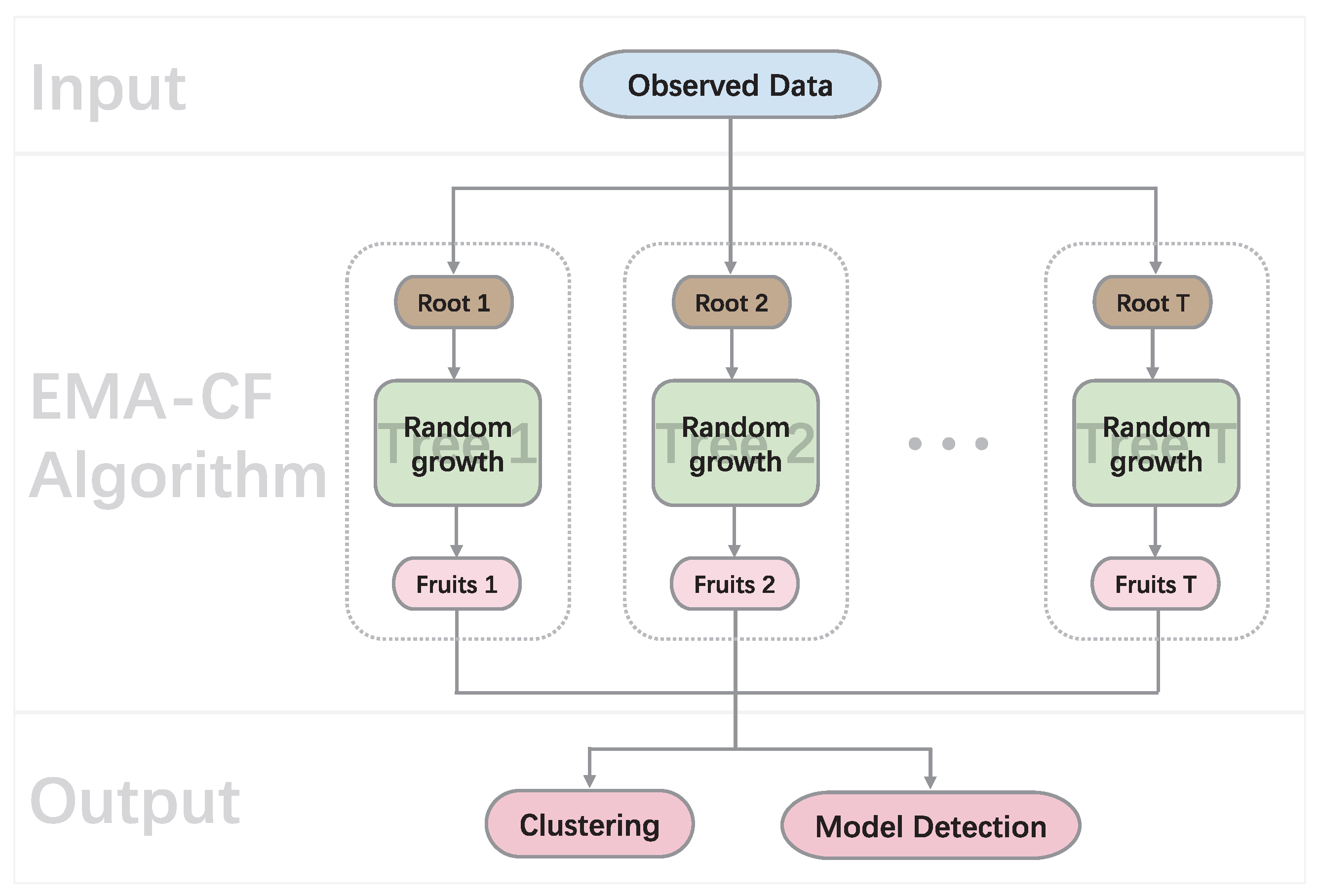
${\mathbf{EO}}^{*}$ denotes the maximum value of $\mathbf{EO}(j,j^{\prime })$ over $1\le j<j^{\prime }\le d$. The normalized quantity $\overline{\mathbf{EO}}(j,j^{\prime })$ lies in $[0,1]$. The higher the value, the stronger the contribution of the conditional dependence between feature j and $j^{\prime }$. The overall CF architecture is summarized in Algorithm 3. Figure 1 provides an overall working flow for model-based clustering based on the EMA-CF algorithm, where the T clustering trees are growing in parallel.

Algorithm 3 The EMA-CF algorithm

1: for$h=1$to T do 2:     Grow a clustering vector ${\tilde{\mathit{s}}}^{\left(h\right)}$ according to Algorithm 2 and obtain the Gaussian graphical model $s_{{\kappa }_1^{\left(h\right)}}^{\left(h\right)}$; 3:     Apply the EMA algorithm under the partition set ${\tilde{\mathit{s}}}^{\left(h\right)}$; 4:     Construct the $n\times n$ consensus matrix ${\mathbf{P}}^{\left(h\right)}$ according to (35); 5:     Compute the vector ${\mathbf{FI}}^{\left(h\right)}$ of feature’s importance according to (36); 6: end for 7: Average ${\mathbf{P}}^{\left(h\right)}$ to get $\overline{\mathbf{P}}⟵{\displaystyle \frac{1}{T}}{\sum }_{h=1}^T{\mathbf{P}}^{\left(h\right)}$ and apply the hierarchical clustering algorithm based on $\mathbf{B}={\mathbf{I}}_n-\overline{\mathbf{P}}$ to get the final clustering; 8: Compute the pattern of feature’s importance as $\overline{\mathbf{FI}}⟵{\displaystyle \frac{1}{T}}{\sum }_{h=1}^T{\mathbf{FI}}^{\left(h\right)}$; 9: Compute the normalized occurrence matrix $\overline{\mathbf{EO}}$ according to (38) for covariance structure detection.

Based on the principle of the EMA-CF algorithm, each cluster instance in the CF architecture has a maximum real-time complexity of $O[n·K^2·d·{\left({\kappa }_1^{*}\right)}^2·IterMax]$ when using ${\kappa }_1^{*}<d^{{\displaystyle \frac{1}{2}}}$. Meanwhile, the real-time complexity of only applying the EMA algorithm is $O[n·K^2·d·IterMax]$. The increased complexity is due to replacement of the naïve Bayes assumption with the LAN assumption to consider within-component correlations.

6. Experiment Study

6.1. Experiments on Synthetic Data

In this section, we assess the proposed parsimonious modeling and approximated BMA approach for model-based clustering through different simulated data scenarios. The objective is to evaluate the ability of this framework to recover the original grouping of the data, as well as its ability to select features and detect covariance structures. We refer to the proposed method for clustering and model detection as EMA-CF.

Eight state-of-the-art model-based clustering methods were chosen for comparison. They are closely related to the proposed one and summarized in

Table 1. The model-based clustering methods under comparison.

Method	Assumption	Purpose
		Clustering	Feature Selection	Covariance Structure Detection
EMA-CF	leaf-augmented naïve Bayes	✓	✓	✓
EMA-naïve	naïve Bayes	✓	✓
MBIC	naïve Bayes	✓	✓
MICL	naïve Bayes	✓	✓
mcgStep	covariance graphs	✓		✓
mclust-BIC	geometric properties	✓		✓
mclust-RMA	geometric properties	✓		✓
mclust-PMA	geometric properties	✓		✓

. To the best of our knowledge, except the proposed method, there are few approaches to performing clustering, feature selection, and covariance structure detection simultaneously. The MBIC method suggested in [49] uses the structural EM algorithm combined with the BIC to realize simultaneous feature selection and clustering in Gaussian mixture models. The MICL method proposed in [21] further tackles parameter uncertainty by considering the ICL, where an alternating optimization algorithm has been designed to find the data separation and distinctive features. Both MBIC and MICL are established on the local independence assumption. They were implemented using the R package “VarSelLCM”. The mcgStep method [15] directly seeks the sparse pattern of the component covariance matrices using the structural EM algorithm. Stepwise searching is required in each iteration to refine the component covariance graphs. The mcgStep method was implemented using the R package “mixggm” with the BIC model selection criterion. The mclust approach [50] in the R package “mclust” is based on the Gaussian parsimonious clustering model (GPCM) family, which is composed of 14 component covariance matrix structures under different levels of constraints after eigenvalue decomposition. mclust-BIC conducts model selection based on the BIC value after the fitting of each model. mclust-RMA and mclust-PMA are approximated BMA methods proposed in [27] based on the 14 model structures. While mclust-RMA performs averaging on the response matrices, mclust-PMA takes averaging on the estimated model parameters. When conducting model averaging, the model weights are approximated by normalizing the BIC values. In addition, we included the EMA algorithm in comparison, which takes BMA over only the naïve Bayes structures to investigate the effects of accounting for the within-class associations with the CF architecture. We denote the method as EMA-naïve. (In the Supplementary Materials, by viewing the EMA algorithm as an approximated CVB approach, we provide comparison results with two additional related clustering methods VarFnMS [51] and VarFnMST [3], which are both VB methods based on the naïve Bayes assumption.)

The MBIC, MICL and mcgStep algorithms require initialization of the cluster allocations as well as the model structure. In the R package “VarSelLCM” for MBIC and MICL, each feature is initialized as discriminant or not discriminant via random sampling. The initial class allocations are then provided by the EM algorithm associated with the initial feature discrimination pattern. We set the number of random initializations in the two algorithms as 100. The output was the result with the maximum BIC value for MBIC and maximum ICL for MICL across the 100 initializations. In the packages “mixggm” and “mclust”, the Gaussian model-based hierarchical clustering approach in [52] is used to initialize the class allocations. Initialization of the component covariance graphs for mcgStep is provided by filtering the sample correlation matrix in each class. The EMA-CF and EMA-naïve algorithms only need initialization of the cluster allocations. Like the competitive algorithms, a poor choice of the starting values may make the convergence very slow and obtain a local optimal. Thus, the choice of a good starting class allocation for EMA-CF or MEA-naïve is important. Or, multiple starting points should be tried as in MBIC and MICL. For overall efficiency of the algorithm, we chose to use the result from the k-means clustering algorithm. To implement the EMA-CF algorithm, the number of maximum allowed times of iterations $IterMax$ in the EMA algorithm was fixed at 100 when growing a clustering vector and set as 500 for the final EMA algorithm with the obtained clustering vector. We set the number of paralleled cluster instances as 100. The maximal allowed times of tree growth ${\kappa }_1^{*}$ and the maximal allowed times of consecutive unsuccessful attempts ${\kappa }_0^{*}$ were both set as 5. Further explorations on the CF controllable parameters are given in the Supplementary Materials. The values specified for these parameters are adequate to ensure a stable and good performance of the algorithm in the following simulation settings.

We considered the synthetic data from a bi-component Gaussian mixture model with mixing proportions $\mathit{\tau }=(0.5,0.5)$, composed of ten features. The component mean of class one was ${\mathit{\mu }}_1={({\mu }_{11},{\mu }_{12},0,0,0,0,0,0,0,0)}^T$, where ${\mu }_{11},{\mu }_{12}$ were generated randomly from the uniform distribution $\mathcal{U}(0,1)$. The mean of class two was given by ${\mathit{\mu }}_2={({\mu }_{11}+2.5ϵ,{\mu }_{12}+2.5ϵ,0,0,0,0,0,0,0,0)}^T$. The value $ϵ$ permits us to tune the class overlaps. Six scenarios differentiated by the covariance structures were considered. In Scenarios 1–4, the covariance structures were well-specified with two, three, five, and ten feature blocks from the LAN family. Scenario 4 corresponds to the naïve Bayes configuration. We also took into account the scenarios where the covariance structures were mis-specified as the Toeplitz type matrix and the Erdos–Renyi model [15] in Scenarios 5 and 6. The probability of two features being marginally correlated was set as 0.2 in the Erdos–Renyi specification. We used the same covariance matrix for different mixture components in each scenario. Without loss of generosity, the diagonal elements of each covariance matrix were set as one. The non-zero off-diagonal elements were randomly chosen from the uniform distribution $\mathcal{U}(0.2,0.8)$ submitting to the symmetric and positive definite constraint. Figure 2 exhibits the simulated covariance graphs and the corresponding Gaussian graphical models in the six scenarios. For each scenario, we generated random datasets with different combinations of sample size $n\in \{25,50,75,100\}$ and class overlap $ϵ\in \{1.0,1.1,1.3,1.6,2.0\}$, and we replicated each experiment twenty times.

As the true class assignment of the synthetic dataset was known, we computed the classification error rate to evaluate the quality of the clustering obtained by the competitive algorithms. The results averaged over the twenty replicates are reported in

Table 2. Classification error rates obtained by the clustering algorithms under comparison in the six scenarios with different sample sizes and class overlaps.

Scenario	Method	$\mathit{ϵ}=1.0$				$\mathit{ϵ}=1.1$				$\mathit{ϵ}=1.3$				$\mathit{ϵ}=1.6$				$\mathit{ϵ}=2.0$
		$\mathit{n}=\mathbf{25}$	$\mathit{n}=\mathbf{50}$	$\mathit{n}=\mathbf{75}$	$\mathit{n}=\mathbf{100}$	$\mathit{n}=\mathbf{25}$	$\mathit{n}=\mathbf{50}$	$\mathit{n}=\mathbf{75}$	$\mathit{n}=\mathbf{100}$	$\mathit{n}=\mathbf{25}$	$\mathit{n}=\mathbf{50}$	$\mathit{n}=\mathbf{75}$	$\mathit{n}=\mathbf{100}$	$\mathit{n}=\mathbf{25}$	$\mathit{n}=\mathbf{50}$	$\mathit{n}=\mathbf{75}$	$\mathit{n}=\mathbf{100}$	$\mathit{n}=\mathbf{25}$	$\mathit{n}=\mathbf{50}$	$\mathit{n}=\mathbf{75}$	$\mathit{n}=\mathbf{100}$
Scen.1	EMA-CF	0.16	0.10	0.10	0.11	0.09	0.09	0.07	0.06	0.03	0.03	0.01	0.01	0.01	0.00	0.00	0.00	0.00	0.00	0.00	0.00
	EMA-naïve	0.20	0.11	0.11	0.15	0.13	0.09	0.07	0.08	0.05	0.04	0.03	0.02	0.02	0.01	0.01	0.01	0.00	0.00	0.00	0.00
	MBIC	0.31	0.34	0.38	0.45	0.30	0.28	0.32	0.39	0.16	0.14	0.15	0.18	0.05	0.05	0.05	0.03	0.02	0.00	0.00	0.00
	MICL	0.24	0.25	0.32	0.40	0.18	0.18	0.28	0.32	0.07	0.08	0.08	0.16	0.03	0.03	0.01	0.03	0.00	0.00	0.00	0.00
	mcgStep	0.16	0.16	0.16	0.10	0.10	0.09	0.13	0.04	0.06	0.02	0.01	0.02	0.01	0.01	0.00	0.00	0.00	0.00	0.00	0.00
	mclust-BIC	0.29	0.30	0.25	0.32	0.22	0.24	0.24	0.22	0.18	0.22	0.21	0.15	0.11	0.10	0.09	0.11	0.05	0.10	0.07	0.00
	mclust-RMA	0.26	0.34	0.24	0.22	0.21	0.30	0.20	0.23	0.21	0.25	0.18	0.15	0.13	0.18	0.07	0.08	0.10	0.16	0.05	0.04
	mclust-PMA	0.26	0.34	0.24	0.22	0.21	0.31	0.20	0.23	0.21	0.25	0.17	0.15	0.13	0.18	0.07	0.08	0.10	0.16	0.05	0.04
Scen.2	EMA-CF	0.06	0.11	0.08	0.06	0.05	0.05	0.05	0.04	0.01	0.03	0.01	0.01	0.01	0.01	0.01	0.00	0.01	0.00	0.00	0.00
	EMA-naïve	0.09	0.10	0.09	0.08	0.03	0.07	0.05	0.05	0.02	0.03	0.02	0.02	0.01	0.01	0.01	0.01	0.01	0.00	0.00	0.00
	MBIC	0.25	0.24	0.13	0.26	0.17	0.11	0.09	0.19	0.08	0.06	0.06	0.05	0.03	0.01	0.01	0.01	0.01	0.00	0.00	0.00
	MICL	0.17	0.20	0.13	0.22	0.10	0.08	0.09	0.13	0.02	0.05	0.04	0.02	0.01	0.01	0.01	0.01	0.01	0.00	0.00	0.00
	mcgStep	0.12	0.10	0.13	0.10	0.11	0.05	0.05	0.06	0.06	0.03	0.02	0.01	0.03	0.01	0.01	0.00	0.00	0.00	0.00	0.00
	mclust-BIC	0.20	0.17	0.28	0.28	0.19	0.18	0.25	0.21	0.15	0.10	0.14	0.14	0.02	0.03	0.11	0.06	0.00	0.00	0.02	0.04
	mclust-RMA	0.18	0.18	0.23	0.25	0.13	0.20	0.23	0.17	0.07	0.08	0.12	0.04	0.06	0.05	0.02	0.05	0.04	0.02	0.00	0.05
	mclust-PMA	0.18	0.18	0.23	0.25	0.12	0.20	0.23	0.17	0.07	0.08	0.12	0.04	0.06	0.06	0.02	0.05	0.04	0.02	0.00	0.05
Scen.3	EMA-CF	0.07	0.08	0.07	0.06	0.05	0.05	0.05	0.05	0.04	0.03	0.02	0.02	0.02	0.01	0.01	0.01	0.01	0.00	0.00	0.00
	EMA-naïve	0.07	0.08	0.07	0.06	0.05	0.06	0.05	0.05	0.04	0.03	0.02	0.02	0.02	0.01	0.01	0.01	0.01	0.00	0.00	0.00
	MBIC	0.20	0.15	0.07	0.06	0.16	0.07	0.05	0.05	0.09	0.05	0.02	0.02	0.04	0.01	0.01	0.01	0.01	0.00	0.00	0.00
	MICL	0.16	0.14	0.07	0.06	0.07	0.08	0.05	0.05	0.03	0.03	0.02	0.02	0.02	0.01	0.01	0.01	0.01	0.00	0.00	0.00
	mcgStep	0.10	0.12	0.13	0.13	0.07	0.09	0.09	0.08	0.04	0.05	0.05	0.03	0.02	0.02	0.01	0.01	0.00	0.01	0.00	0.00
	mclust-BIC	0.14	0.10	0.07	0.06	0.09	0.08	0.05	0.04	0.06	0.03	0.02	0.02	0.03	0.01	0.01	0.00	0.00	0.00	0.00	0.00
	mclust-RMA	0.13	0.10	0.07	0.06	0.09	0.08	0.05	0.04	0.06	0.03	0.02	0.02	0.03	0.01	0.01	0.00	0.00	0.00	0.00	0.00
	mclust-PMA	0.13	0.10	0.07	0.07	0.09	0.08	0.05	0.04	0.06	0.03	0.02	0.02	0.03	0.01	0.01	0.00	0.00	0.00	0.00	0.00
Scen.4	EMA-CF	0.12	0.06	0.05	0.05	0.06	0.04	0.04	0.04	0.02	0.02	0.02	0.01	0.01	0.00	0.01	0.00	0.00	0.00	0.00	0.00
	EMA-naïve	0.11	0.06	0.05	0.05	0.06	0.04	0.04	0.04	0.02	0.02	0.02	0.01	0.01	0.00	0.01	0.00	0.00	0.00	0.00	0.00
	MBIC	0.25	0.06	0.05	0.05	0.18	0.04	0.04	0.04	0.02	0.02	0.02	0.01	0.01	0.00	0.01	0.00	0.00	0.00	0.00	0.00
	MICL	0.14	0.06	0.05	0.05	0.10	0.04	0.04	0.04	0.02	0.02	0.02	0.01	0.01	0.00	0.01	0.00	0.00	0.00	0.00	0.00
	mcgStep	0.09	0.09	0.06	0.07	0.07	0.06	0.04	0.05	0.03	0.03	0.02	0.02	0.00	0.01	0.00	0.01	0.00	0.00	0.00	0.00
	mclust-BIC	0.16	0.05	0.04	0.05	0.13	0.03	0.03	0.04	0.06	0.02	0.01	0.02	0.05	0.00	0.00	0.00	0.02	0.00	0.00	0.00
	mclust-RMA	0.15	0.06	0.05	0.05	0.11	0.04	0.04	0.03	0.04	0.01	0.01	0.02	0.00	0.00	0.00	0.00	0.00	0.00	0.00	0.00
	mclust-PMA	0.14	0.06	0.05	0.05	0.11	0.04	0.04	0.03	0.04	0.01	0.01	0.02	0.00	0.00	0.00	0.00	0.00	0.00	0.00	0.00
Scen.5	EMA-CF	0.12	0.07	0.07	0.05	0.07	0.06	0.04	0.04	0.04	0.03	0.02	0.02	0.02	0.01	0.00	0.00	0.01	0.00	0.00	0.00
	EMA-naïve	0.12	0.08	0.06	0.07	0.09	0.06	0.04	0.05	0.03	0.02	0.02	0.03	0.01	0.01	0.01	0.01	0.00	0.00	0.00	0.00
	MBIC	0.23	0.13	0.06	0.07	0.20	0.07	0.04	0.05	0.07	0.03	0.02	0.03	0.01	0.01	0.01	0.01	0.00	0.00	0.00	0.00
	MICL	0.16	0.11	0.06	0.07	0.09	0.07	0.04	0.05	0.02	0.03	0.02	0.03	0.01	0.01	0.01	0.01	0.00	0.00	0.00	0.00
	mcgStep	0.12	0.11	0.08	0.06	0.10	0.07	0.05	0.02	0.05	0.04	0.01	0.01	0.02	0.01	0.00	0.00	0.01	0.00	0.00	0.00
	mclust-BIC	0.21	0.31	0.29	0.26	0.16	0.21	0.24	0.16	0.10	0.16	0.17	0.13	0.08	0.05	0.06	0.04	0.05	0.03	0.02	0.04
	mclust-RMA	0.21	0.30	0.30	0.25	0.16	0.20	0.24	0.16	0.10	0.16	0.17	0.13	0.08	0.05	0.06	0.04	0.05	0.03	0.02	0.04
	mclust-PMA	0.20	0.30	0.29	0.25	0.16	0.21	0.24	0.16	0.10	0.16	0.17	0.13	0.08	0.05	0.06	0.04	0.05	0.03	0.02	0.04
Scen.6	EMA-CF	0.09	0.06	0.05	0.05	0.05	0.03	0.02	0.03	0.02	0.01	0.01	0.01	0.00	0.00	0.01	0.00	0.00	0.00	0.00	0.00
	EMA-naïve	0.10	0.08	0.05	0.04	0.06	0.04	0.03	0.03	0.03	0.02	0.01	0.01	0.01	0.00	0.00	0.00	0.00	0.00	0.00	0.00
	MBIC	0.20	0.13	0.08	0.06	0.10	0.05	0.03	0.03	0.07	0.02	0.01	0.01	0.01	0.00	0.00	0.00	0.00	0.00	0.00	0.00
	MICL	0.12	0.08	0.07	0.04	0.04	0.04	0.03	0.03	0.02	0.01	0.01	0.01	0.01	0.00	0.00	0.00	0.00	0.00	0.00	0.00
	mcgStep	0.10	0.09	0.04	0.00	0.07	0.05	0.02	0.00	0.03	0.01	0.00	0.00	0.00	0.00	0.00	0.00	0.00	0.00	0.00	0.00
	mclust-BIC	0.16	0.15	0.13	0.10	0.14	0.15	0.18	0.08	0.06	0.09	0.05	0.04	0.03	0.03	0.00	0.08	0.03	0.00	0.00	0.00
	mclust-RMA	0.15	0.15	0.13	0.10	0.14	0.15	0.18	0.08	0.06	0.11	0.05	0.04	0.03	0.03	0.00	0.08	0.03	0.00	0.00	0.00
	mclust-PMA	0.16	0.15	0.13	0.10	0.13	0.14	0.18	0.08	0.06	0.11	0.05	0.04	0.03	0.03	0.00	0.08	0.03	0.00	0.00	0.00

. The first and the second smallest classification error rates in each case are marked in bold. Table S3 provides the results of the standard deviation of the classification error rates. In general, the EMA-CF method outperforms the others and shows robustness across various simulation settings. The performance gain is substantial when the within-component correlation is strong, such as in Scenarios 1 and 2. It is noticeable that the mcgStep method also obtains relatively small classification errors in these scenarios, which emphasizes the importance of modeling the component covariance structures when presumptively high association relationships are present in the data. For small class overlap $ϵ=2.0$, all the methods tend to attain an almost perfect classification of the data. The EMA-CF method improves the data separation dramatically when the class overlap is increased. While EMA-CF improves the performance of EMA-naïve in Scenarios 1 and 2 when the within-component correlation is strong, the two methods show an overall competitive performance in the remaining four scenarios. Moreover, the EMA-naïve method outperforms MBIC and MICL when the class overlap is high. While the three methods all assume the naïve Bayes network structure, EMA-naïve considers the model uncertainty by employing the BMA.

The predictive log score (PLS) [25] is defined by

$${\mathrm{PLS}}_{target}=-\sum _{i_0=1}^{n_0}log{p}_{target}({\mathit{z}}_{i_0},{\mathit{x}}_{i_0}),$$

(39)

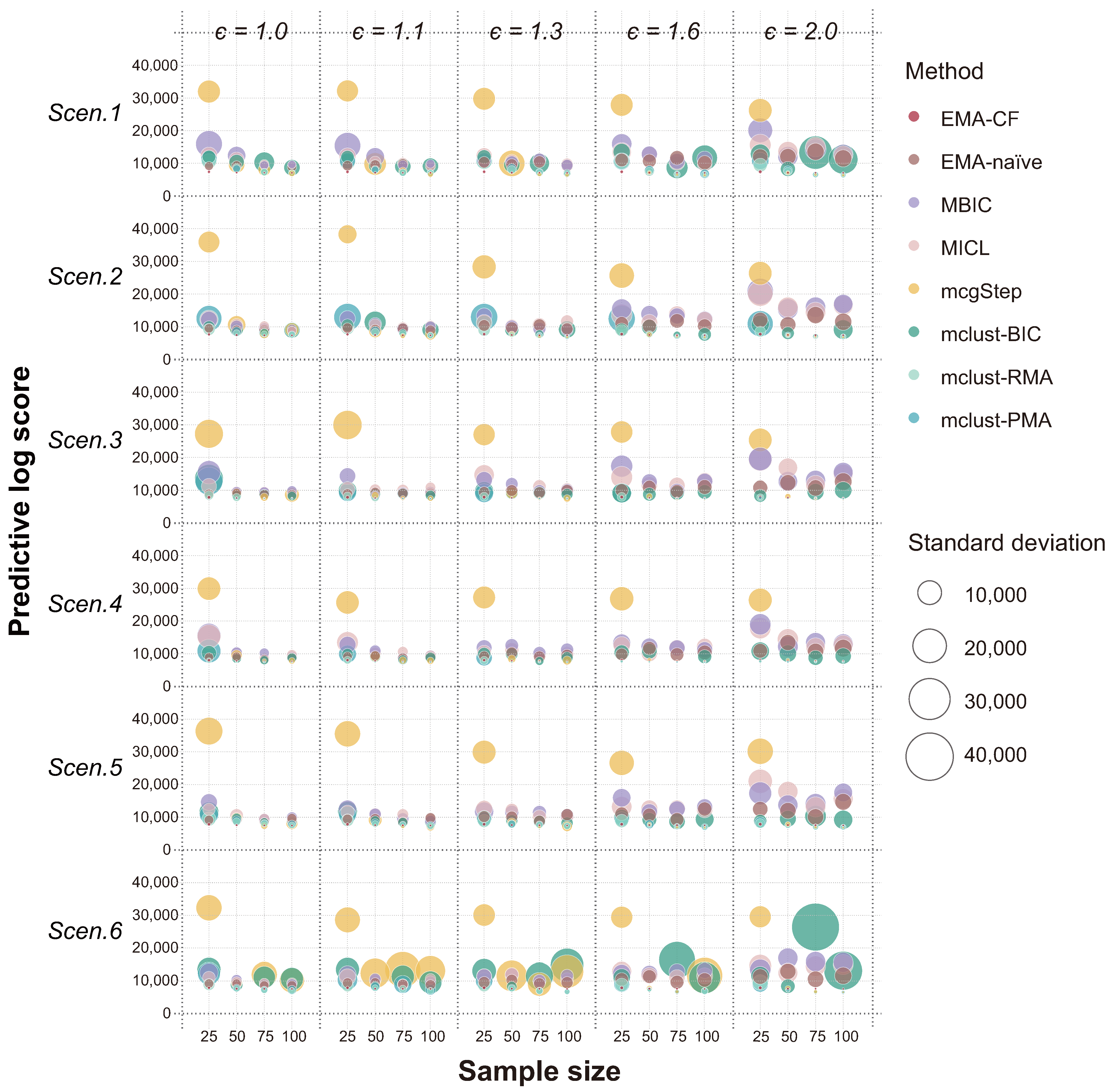
where ${\{{\mathit{z}}_{i_0},{\mathit{x}}_{i_0}\}}_{i_0=1}^{n_0}$ is the set of testing data and $p_{target}({\mathit{z}}_{i_0},{\mathit{x}}_{i_0})$ denotes the predictive probability on datum $({\mathit{z}}_{i_0},{\mathit{x}}_{i_0})$ given in the target method. Following the logarithmic scoring rule of Good [23], a better modeling strategy should consistently assign higher probabilities to the events that actually occur. Therefore, the smaller the PLS, the more reliable the method. The results of PLS obtained using the eight methods in the six scenarios are compared in the bubble plot shown in Figure 3. The radius of each circle indicates the variation of the PLS values over the twenty replicates. The EMA-CF method shows remarkably high predicting performance across different covariance structure configurations. And, the results are robust across various simulation settings. Particularly, using EMA-CF reduces the PLS of EMA-naïve in each case, which suggests the significance of modeling the within-component correlations.

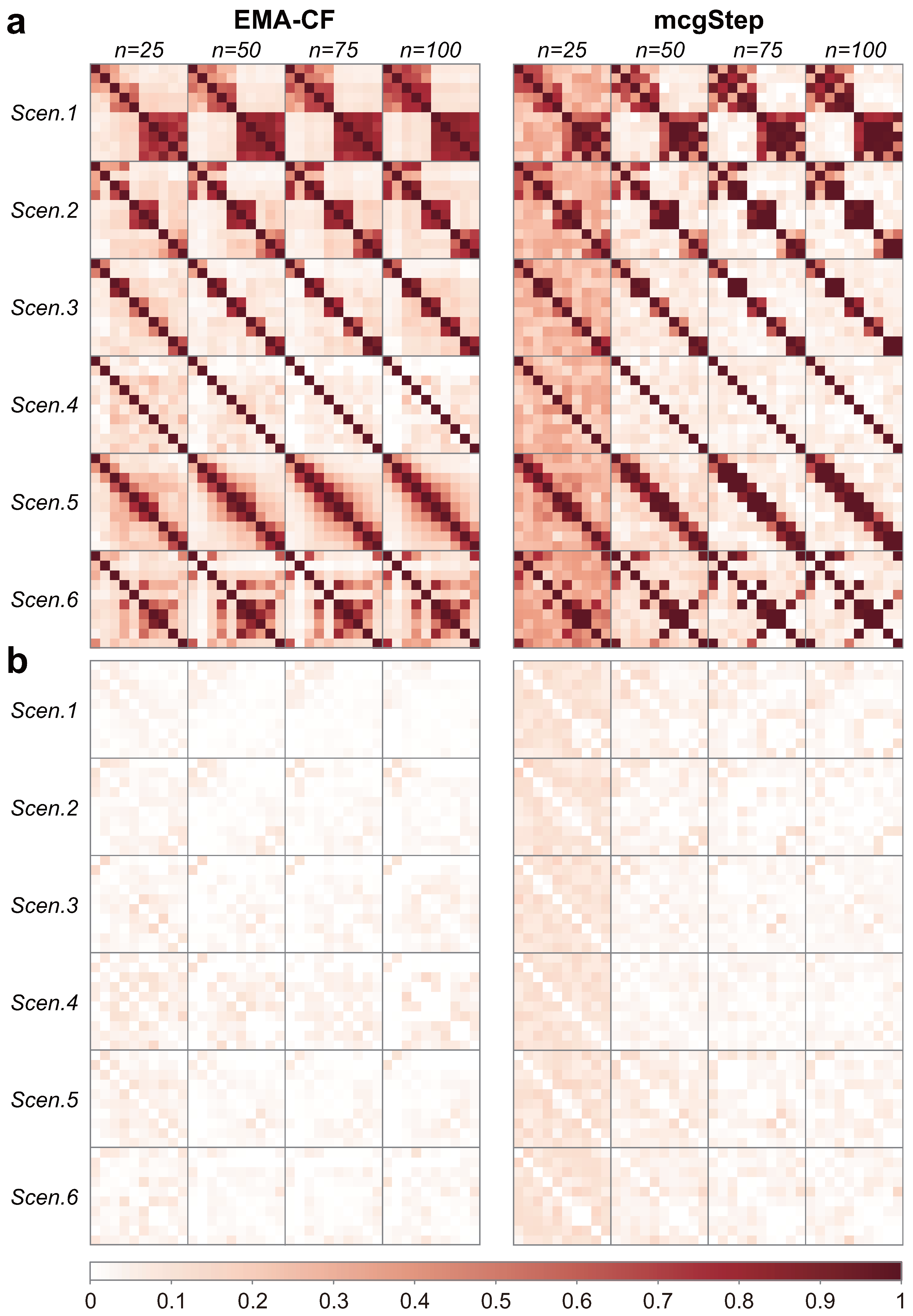
The covariance structure detection ability was compared between EMA-CF, mcgStep, and mclust-BIC, and the ability to identify the feature importance pattern was compared between EMA-CF, EMA-naïve, MBIC, and MICL. Figure 4 shows the covariance structures detected using the EMA-CF and mcgStep methods. As the results are not sensitive to the class overlap, only the cases with $ϵ=1.3$ are illustrated here. The remaining results are present in the Supplementary Materials. While the mcgStep method gives an estimation of the covariance structure as the covariance graph, EMA-CF provides an estimation as the Gaussian graphical model. Both methods show good performance in detecting the underlying graph configurations. The EMA-CF method exhibits more robustness, especially when the sample size is small. The covariance structures detected most frequently over the twenty replicates by the mclust-BIC method are shown in

Table 3. Covariance structure detection by mclust-BIC in the six scenarios with the class overlap setting $ϵ=1.3$.

Scenario	$\mathit{n}=25$	$\mathit{n}=50$	$\mathit{n}=75$	$\mathit{n}=100$
Scen.1	EEE 1 (6)	EEE (13)	EEE (12)	EEE (13)
Scen.2	EII 2 (7)	EII (9)	EEE (14)	EEE (17)
Scen.3	EII (14)	EII (17)	EII (17)	EII (19)
Scen.4	EII (17)	EII (18)	EII (18)	EII (20)
Scen.5	EII (14)	EEE (7)	EEE (13)	EEE (15)
Scen.6	EII (13)	EII (11)	EEE (14)	EEE (15)

¹ This is a model from the GPCM family with equal volume, shape, and orientation parameters across the components. ² This is a model from the GPCM family with equal volume and shape parameters across the components but no orientation parameters.

. The detection frequency is present within the parentheses. The EII structure indicates that the component covariance matrices are diagonal and homogeneous. EEE indicates a homogeneous full covariance structure for the components.

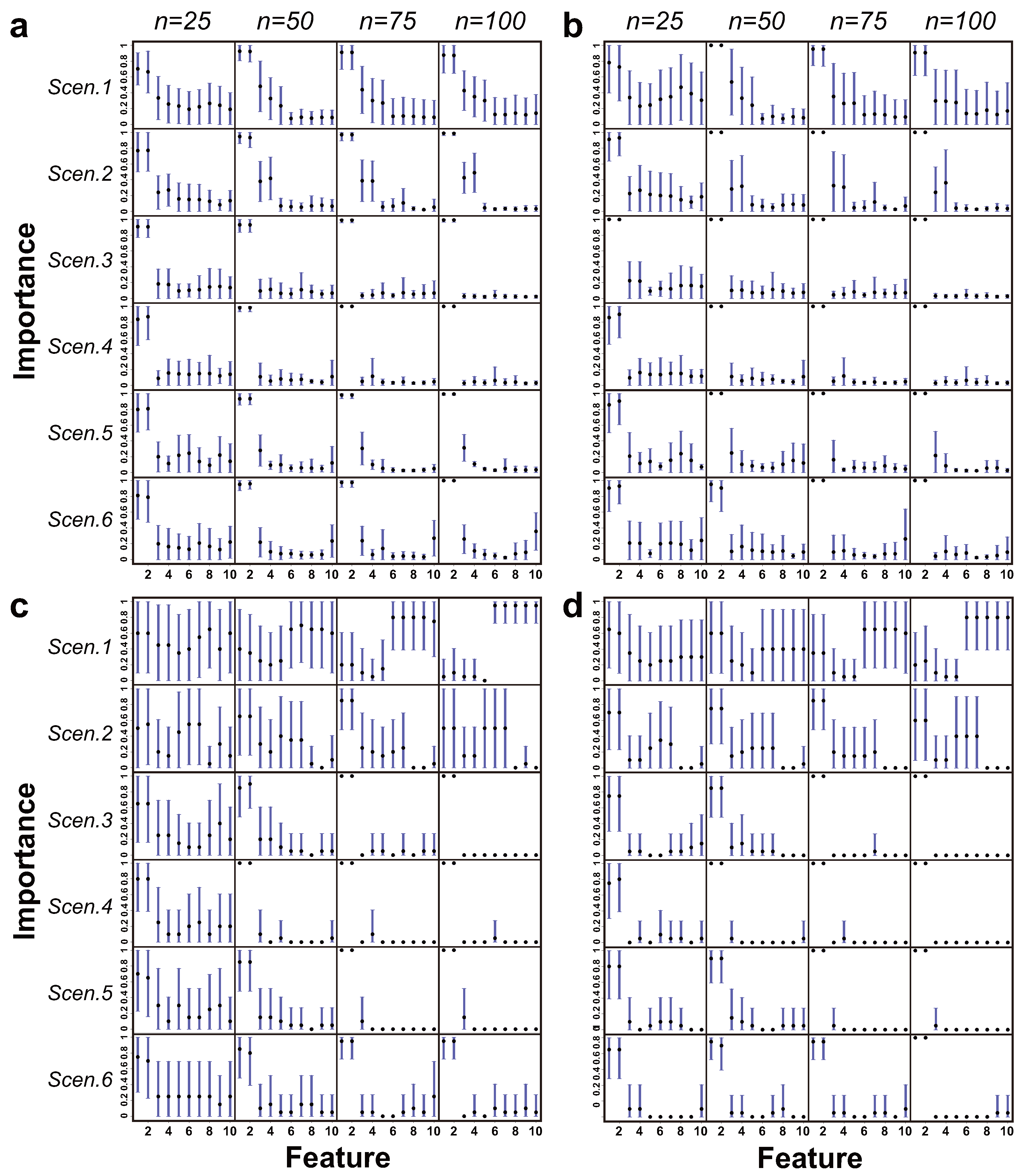
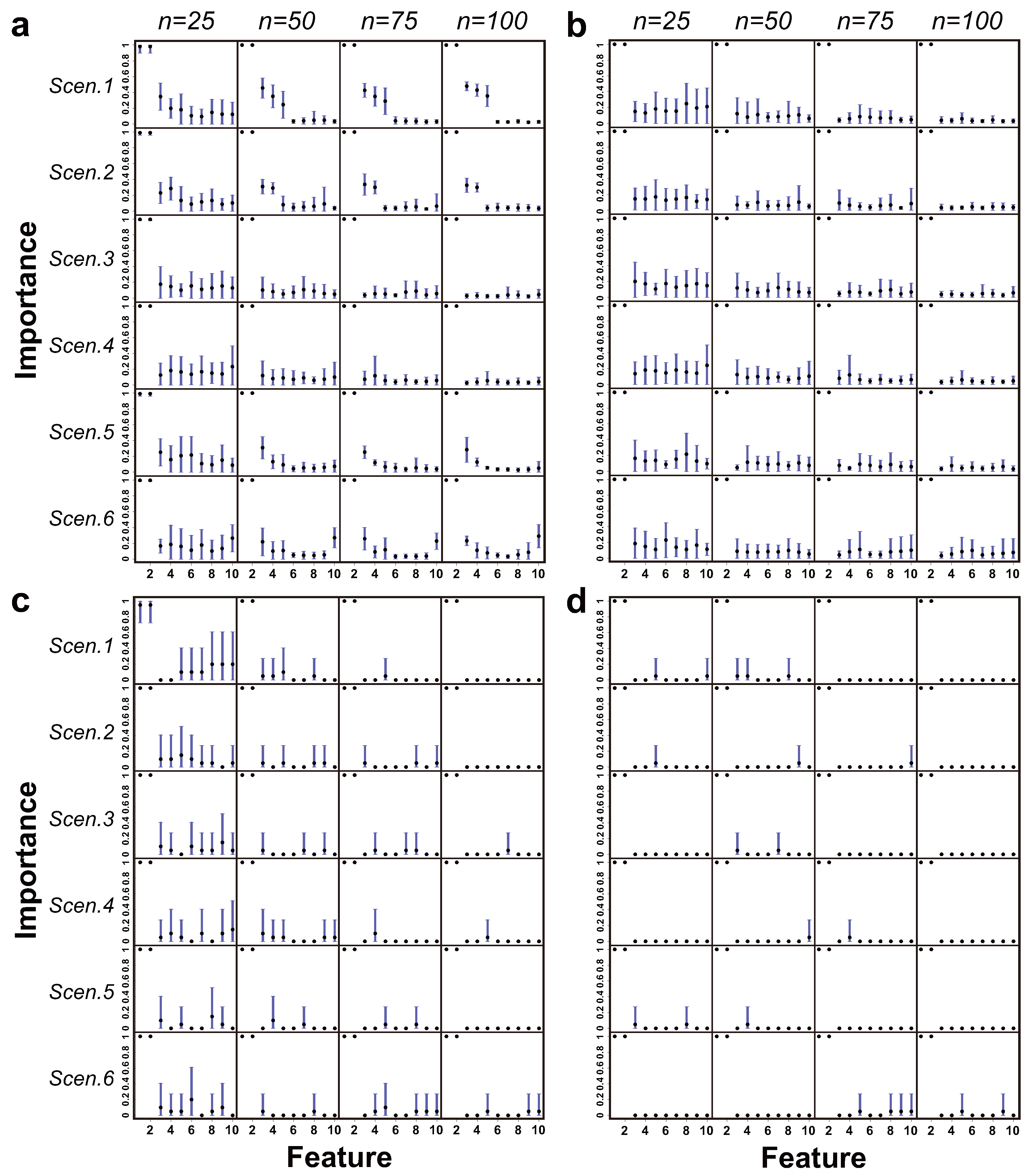
Figure 5, Figure 6 and Figure 7 show the patterns of feature importance estimated by the EMA-CF, EMA-naïve, MBIC, and MICL methods under class overlap settings of $ϵ\in \{1.0,1.3,2.0\}$, respectively. The cases for $ϵ\in \{1.1,1.6\}$ are present in the Supplementary Materials. Overall, the results of EMA-CF show great robustness, responsive to the corresponding association structures between features. It is noticeable that the estimated patterns of feature importance for Scenarios 1 and 2 by EMA-CF are distinguished from those estimated by EMA-naïve, MBIC, and MICL. The difference becomes evident as the class overlap decreases and the sample size increases. Indeed, the associations of the last eight features with the first two induce their indirect contributions to the classification. The MBIC and MICL methods perform erratically in Scenarios 1 and 2 when the class overlap is high. In Scenarios 3 and 4, where there is no conditional association between the first two and the remaining eight features, the four methods give similar identification results. In Scenarios 5 and 6, where the structures assumed are not from the LAN family, EMA-CF detects some latent patterns of the feature’s significance induced by the simulated association structures. Overall, EMA-CF and EMA-naïve, which are based on the BMA, show consistency behaviors as the sample size increases. Such behaviors are conformable to the principle of BMA, where the probability mass function of model structures (model weights) peaks gradually at the MAP structure as the size of the dataset increases [31].

6.2. Experiments on Real-World Datasets

In this section, we illustrate the proposed method by applying it to some benchmark datasets: Iris, Olive, Wine, and Digit. The Iris dataset was obtained from the R package “datasets”. Olive is the Italian olive oil dataset and Wine the Italian wine dataset. They were both obtained from the R package “pgmm”. The Digit dataset was obtained from the UCI machine learning repository (https://doi.org/10.24432/C50P49; accessed on 26 August 2025). The complete data of Digit contain more than 5000 images for the handwritten digits 0–9. They are gray-scale with a size of $8\times 8$ pixels. We focused on separation of the 4 and 9 digits and randomly reserved 100 images for each digit. As the variability of some pixels for a digit was exactly zero, singularity problems could occur in the model-based clustering algorithms. Therefore, we put a noise mask on the data matrix (of size $200\times 64$). Each element of the noise mask was generated from $\mathcal{N}(0,0.1)$.

Table 4. Basic information for the four benchmark datasets.

Dataset	Iris	Olive	Wine	Digit
K	3	3	3	2
d	4	8	27	64
n	150	572	178	200

presents the basic information for the four datasets.

To implement the EMA-CF method, as we had little information about the covariance structure of the data, we varied the setting of ${\kappa }_1^{*}$ that controls the tree growth in the CF architecture between $d^{{\displaystyle \frac{1}{4}}}$, $d^{{\displaystyle \frac{1}{2}}}$ and $d^{{\displaystyle \frac{3}{4}}}$ (rounded to the nearest integer) to match with different levels of sparsity. We denote the corresponding EMA-CF algorithms as EMA-CF-1, EMA-CF-2, and EMA-CF-3, respectively. The number of cluster instances was fixed at $T=100$, and let ${\kappa }_0^{*}=5$. We kept the settings of the other algorithms the same as those in the simulation study.

The clustering quality was evaluated by comparing it with the original grouping of the data.

Table 5. Classification error rates obtained using the clustering methods under comparison for the four benchmark datasets.

Method	Iris	Olive	Wine	Digit
EMA-CF-1	0.040	0.245	0.045	0.060
EMA-CF-2	0.033	0.245	0.045	0.060
EMA-CF-3	0.033	0.066	0.045	0.060
EMA-naïve	0.100	0.245	0.045	0.060
MBIC	0.393	0.453	0.056	0.090
MICL	0.393	0.453	0.056	0.100
mcgStep	0.087	0.180	0.236	0.140
mclust-BIC	0.033	0.390	0.056	0.495
mclust-RMA	0.033	0.339	0.056	0.495
mclust-PMA	0.033	0.339	0.056	0.495

shows the classification errors obtained by the eight competing methods. In general, the EMA-CF method gives the lowest classification errors for all the four datasets. For the Wine and Digit datasets, the best results can be achieved when ${\kappa }_1^{*}$ is small, and the EMA-naïve method that does not model the covariance structure performs equally well. Larger ${\kappa }_1^{*}$ values improve data separation for the Iris and Olive datasets. The MBIC and MICL methods based on the conditional independence assumption provide the worst results for Iris and Olive, but they show sound performance for Wine and Digit. The mcgStep method provides relatively good classification for Iris and Olive but is undesirable for Wine and Digit.

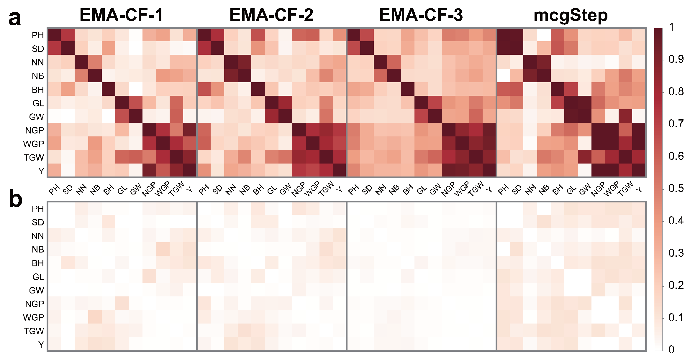
Figure 8 shows the covariance structures detected by EMA-CF and mcgStep. The two methods both advocate strong within-class correlations in Iris and Olive. Even with a small ${\kappa }_1^{*}$ value, the overall color of the normalized occurrence matrix given by EMA-CF is remarkably deep. In contrast, the associations in Wine and Digit are much sparser. The covariance structures given by the mclust-BIC method are VEV, EVV, EVI, and EEE for Iris, Olive, Wine, and Digit, respectively. While EVI indicates diagonal component covariance matrices, VEV, EVV, and EEE produce full covariance matrices. The combined results with the classification performance indicate that the EMA-CF method can accommodate various kinds of covariance structures and give more reliable clustering results.

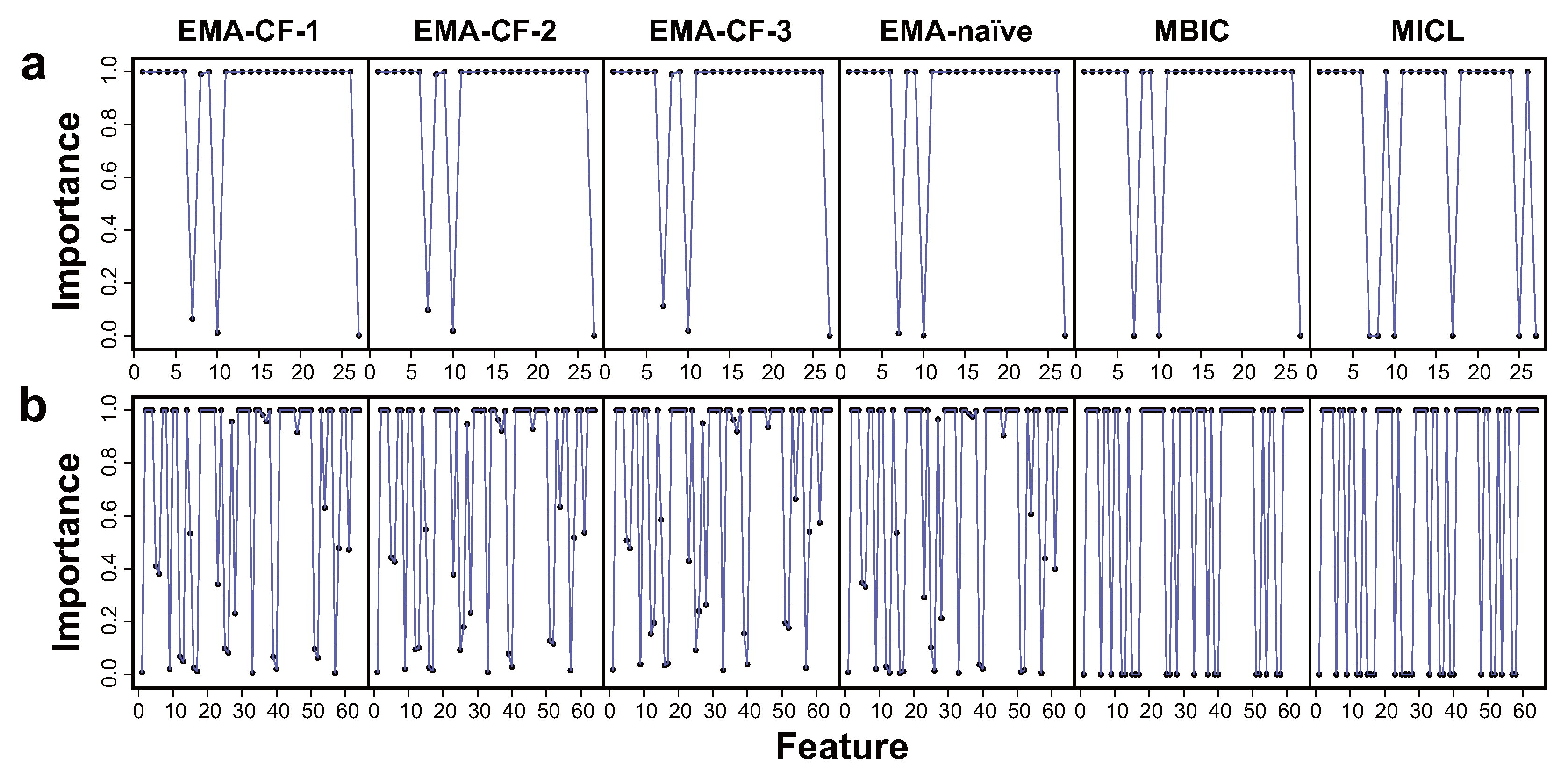
Implementation of EMA-CF, EMA-naïve, MBIC, and MICL gives the estimated patterns of feature importance. For Iris and Olive, the four methods have the same identification, where all the features are significant at the highest level (see Figure S11 in the Supplementary Materials). The results for Wine and Digit are compared in Figure 9. While the MBIC and MICL methods separate the features as discriminating and undiscriminating, EMA-CF and EMA-naïve give relatively conservative estimations of feature importance by taking into account model uncertainty with BMA. There are no apparent differences between the results of EMA-CF andEMA-naïve, which agrees with the sparse patterns of feature association in the two datasets, as detected in Figure 8.

6.3. Application on Tartary Buckwheat Data

In this section, we present an application of the developed method in a real agriculture problem. The data reflect a traditional edible and medicinal crop, Tartary buckwheat. The experimental data contain a total of 200 Tartary buckwheat landraces growing in two different locations with distinct climate conditions [53], denoted as E1 and E2, respectively. Eleven phenotypic traits of the Tartary buckwheat plant were investigated:

• plant morphological traits
  plant height (PH), stem diameter (SD), number of nodes (NN), number of branches (NB), and branch height (BH)
• grain-related traits
  grain length (GL) and grain width (GW)
• yield-related traits
  number of grains per plant (NGP), weight of grains per plant (WGP), 1000-grain weight (TGW), and yield per hectare (Y)

It is commonly acknowledged that changing environment has non-negligible impacts on the growth and development of crops. Our study is concerned with the influence of environmental changes on the Tartary buckwheat landraces. We mixed the phenotypic data of 100 randomly selected landraces from environments E1 and E2. The experiment was repeated twenty times. Again, in using the EMA-CF method, we set ${\kappa }_1^{*}$ as $d^{{\displaystyle \frac{1}{4}}}$, $d^{{\displaystyle \frac{1}{2}}}$, and $d^{{\displaystyle \frac{3}{4}}}$. In each of the eight competing methods, a bi-component clustering model was constructed. Therefore, major impacts of the environmental changes could be confirmed by separation of the data according to their original environments.

Table 6. Classification error rates and predictive log scores (PLS) obtained using the clustering methods under comparison.

Method	Error	PLS
EMA-CF-1	0.108 (0.035)	6064 (259)
EMA-CF-2	0.102 (0.044)	5917 (315)
EMA-CF-3	0.080 (0.050)	5294 (290)
EMA-naïve	0.104 (0.034)	6660 (752)
MBIC	0.108 (0.034)	7427 (1411)
MICL	0.109 (0.034)	7956 (1425)
mcgStep	0.248 (0.150)	6755 (1203)
mclust-BIC	0.234 (0.232)	6307 (1226)
mclust-RMA	0.234 (0.232)	6453 (2391)
mclust-PMA	0.234 (0.232)	5763 (33)

shows the classification errors and the PLS values obtained using the eight methods. The class assignment given by EMA-CF with ${\kappa }_1^{*}=d^{{\displaystyle \frac{3}{4}}}$ shows the highest consistency with the original grouping of the data divided by the environments. Moreover, EMA-CF shows the highest predictive ability compared with the competitive methods.

The covariance structures detected by EMA-CF and mcgStep show strong evidence of the within-class correlations between the phenotypic traits of Tartary buckwheat. As shown in Figure 10, there are heavy associations between the yield-related traits. Moreover, the conditional correlations are evident between PH and SD, between NN and NB, and between GL and GW, as assessed by the EMA-CF method. The phenotype TGW is found to be related to GL and GW, which agrees with the findings in a previous study [54]. The covariance structures provided by mclust-BIC over the twenty replicates are EVE (10 times) and VVE (10 times), both of which indicate full component covariance matrices.

From Figure 11, we can find that all the yield-related traits are discriminant between environments E1 and E2. In addition, the phenotypes PH, SD, BH, and GL are also identified as significant. These facts suggest the sensitivity of the Tartary buckwheat landraces to the environmental changes. While the significance of GW is gradually identified by EMA-CF as ${\kappa }_1^{*}$ increases, it is regarded as unimportant by the EMA-naïve, MBIC, or MICL methods, which have ignored the associations between GW and the yield-related traits.

While most Tartary buckwheat landraces can be separated according to their growing environments (E1 and E2), there are a small group of landraces that are easy to misclassify.

Table 7. Yield and the percentile of yield of the selected landraces in environments E1 and E2.

Landrace	E1		E2
	Y (kg/ha)	Percentile (%)	Y (kg/ha)	Percentile (%)
XZ-1	470.6	61.5	177.1	1.0
GZ-1	583.2	82.0	398.0	4.5
XZ-12	73.5	7.0	370.0	3.5
SNX-15	474.4	62.5	992.0	67.0
SC-8	587.8	82.5	1038.6	73.5
GZ-32	909.3	98.0	1044.2	74.5
SNX-47	486.9	65.5	457.0	7.5

summaries those landraces that have data misclassified into the same class ten times or more across the twenty replicates by the EMA-CF-3 algorithm. Among them, SC-8 and GZ-32 exhibit high yields in both environments, which could provide potentially excellent varieties for further investigation.

7. Conclusions

In this paper, we present a comprehensive framework for model-based clustering. This framework is based on the LAN family for parsimonious modeling of the Gaussian mixtures, which allows for feature selection and covariance structure detection simultaneously. A class of diffused-conjugate priors were proposed to realize objective Bayesian inference. The EMA-CF algorithm was developed to integrate model uncertainty by BMA over the LAN family, which takes advantage of the closed-form expression of the BMA classifier under the naïve Bayes assumption and provides an efficient approximation of model averaging over feature partitions using the ensemble learning strategy of CF.

Extensive experiments on synthetic and real-world datasets showed that the proposed method is able to capture real model structures and exhibits better clustering performance than those relying on the naïve Bayes assumption or solely modeling the association structures. The application of the developed method on the multi-environmental Tartary buckwheat data showed its applicability and usefulness in the agricultural fields. More applications will be explored in our future work.

In the proposed method, we took the number of clusters (number of components in the mixture model) as fixed and given before inference, which however, in most of the situations is unknown a priori. A commonly applied approach is Bayesian model selection from a set of intended numbers with some model selection criterion [17,20,21,49]. In ongoing work, we would like to implement a soft model selection which takes into account model uncertainty regarding the number of mixture components by extending the proposed architecture with an additional level of BMA. Datasets generated with different numbers of mixture components will be experimented on to examine the robustness of this enhanced method for simultaneous clustering and model structure detection.

Additionally, in the synthetic and real-data experiments, we considered the clustering problems mainly of the balanced case, i.e., the clusters are of similar sizes. Like the EM algorithm, a potential problem for EMA in the unbalanced case is the empty components. These could disrupt the execution of the algorithm. A direct and simple remedy is to add a noise mask to the response matrix when the summation of a column in the matrix becomes smaller than a threshold value. Further enhancement could be achieved by utilizing the simulated annealing strategy [55]. More detailed investigation of unbalanced clustering will be present in our subsequent work.

In Section 5, we briefly analyzed the real-time complexity of the EMA-CF algorithm. The additional level of model averaging over the feature partitions would worsen the time complexity but allow for an investigation into the within-component correlations. Indeed, the EMA-CF, mcgStep, and mclust algorithms took relatively longer times to complete the computation during the experiments than the EMA-naïve, MBIC, and MICL algorithms, which only consider the feature selection. Given that the execution time of an algorithm is heavily influenced by the choice of programming language, the performance of the EMA-CF algorithm, which has been initially written in the R language, could be notably enhanced through implementation in C++. As part of our subsequent work, we will rewrite this algorithm in C++ with the goal of significantly improving its efficiency and distributing it systematically as an R package.

References

1. Jiang, Z.; Zheng, Y.; Tan, H.; Tang, B.; Zhou, H. Variational deep embedding: An unsupervised and generative approach to clustering. In Proceedings of the 26th International Joint Conference on Artificial Intelligence, Melbourne, Australia, 19–25 August 2017; pp. 1965–1972. [Google Scholar]
2. Yang, L.; Cheung, N.M.; Li, J.; Fang, J. Deep clustering by Gaussian mixture variational autoencoders with graph embedding. In Proceedings of the 2019 IEEE/CVF International Conference on Computer Vision (ICCV), Seoul, Republic of Korea, 27 October–2 November 2019; pp. 6440–6449. [Google Scholar]
3. Sun, J.; Zhou, A.; Keates, S.; Liao, S. Simultaneous Bayesian clustering and feature selection through student’s t mixtures model. IEEE Trans. Neural Netw. Learn. Syst. 2018, 29, 1187–1199. [Google Scholar] [CrossRef] [PubMed]
4. Bouveyron, C.; Brunet-Saumard, C. Model-based clustering of high-dimensional data: A review. Comput. Stat. Data Anal. 2014, 71, 52–78. [Google Scholar] [CrossRef]
5. Ormoneit, D.; Tresp, V. Averaging, maximum penalized likelihood and Bayesian estimation for improving Gaussian mixture probability density estimates. IEEE Trans. Neural Netw. 1998, 9, 639–650. [Google Scholar] [CrossRef]
6. Law, M.H.C.; Figueiredo, M.A.T.; Jain, A.K. Simultaneous feature selection and clustering using mixture models. IEEE Trans. Pattern Anal. Mach. Intell. 2004, 26, 1154–1166. [Google Scholar] [CrossRef]
7. Li, Y.; Dong, M.; Hua, J. Simultaneous localized feature selection and model detection for Gaussian mixtures. IEEE Trans. Pattern Anal. Mach. Intell. 2009, 31, 953–960. [Google Scholar] [CrossRef]
8. Hong, X.; Li, H.; Miller, P.; Zhou, J.; Li, L.; Crookes, D.; Lu, Y.; Li, X.; Zhou, H. Component-based feature saliency for clustering. IEEE Trans. Knowl. Data Eng. 2021, 33, 882–896. [Google Scholar] [CrossRef]
9. Perthame, E.; Friguet, C.; Causeur, D. Stability of feature selection in classification issues for high-dimensional correlated data. Stat. Comput. 2016, 26, 783–796. [Google Scholar] [CrossRef]
10. Fan, J.; Ke, Y.; Wang, K. Factor-adjusted regularized model selection. J. Econom. 2020, 216, 71–85. [Google Scholar] [CrossRef]
11. Mai, Q.; Zou, H.; Yuan, M. A direct approach to sparse discriminant analysis in ultra-high dimensions. Biometrika 2012, 99, 29–42. [Google Scholar] [CrossRef]
12. Celeux, G.; Govaert, G. Gaussian parsimonious clustering models. Pattern Recognit. 1995, 28, 781–793. [Google Scholar] [CrossRef]
13. McLachlan, G.J.; Bean, R.W.; Jones, L.B.T. Extension of the mixture of factor analyzers model to incorporate the multivariate t-distribution. Comput. Stat. Data Anal. 2007, 51, 5327–5338. [Google Scholar] [CrossRef]
14. Andrews, J.L.; McNicholas, P.D. Extending mixtures of multivariate t-factor analyzers. Stat. Comput. 2011, 21, 361–373. [Google Scholar] [CrossRef]
15. Fop, M.; Murphy, T.B.; Scrucca, L. Model-based clustering with sparse covariance matrices. Stat. Comput. 2019, 29, 791–819. [Google Scholar] [CrossRef]
16. Ruan, L.; Yuan, M.; Zou, H. Regularized parameter estimation in high-dimensional Gaussian mixture models. Neural Comput. 2011, 23, 1605–1622. [Google Scholar] [CrossRef] [PubMed]
17. Galimberti, G.; Soffritti, G. Using conditional independence for parsimonious model-based Gaussian clustering. Stat. Comput. 2013, 23, 625–638. [Google Scholar] [CrossRef]
18. Witten, D.M.; Friedman, J.H.; Simon, N. New insights and faster computations for the graphical lasso. J. Comput. Graphical Stat. 2011, 20, 892–900. [Google Scholar] [CrossRef]
19. Dash, D.; Cooper, G.F. Exact model averaging with naive Bayesian classifiers. In Proceedings of the 19th International Conference on Machine Learning, San Francisco, CA, USA, 8–12 July 2002; pp. 91–98. [Google Scholar]
20. Bhattacharya, S.; McNicholas, P.D. A LASSO-penalized BIC for mixture model selection. Adv. Data Anal. Classif. 2014, 8, 45–61. [Google Scholar] [CrossRef]
21. Marbac, M.; Sedki, M. Variable selection for model-based clustering using the integrated complete-data likelihood. Stat. Comput. 2017, 27, 1049–1063. [Google Scholar] [CrossRef]
22. Crook, O.M.; Gatto, L.; Kirk, P.D.W. Fast approximate inference for variable selection in Dirichlet process mixtures, with an application to pan-cancer proteomics. Stat. Appl. Genet. Mol. Biol. 2019, 18, 20180065. [Google Scholar] [CrossRef]
23. Madigan, D.; Raftery, A.E. Model selection and accounting for model uncertainty in graphical models using Occam’s window. J. Am. Stat. Assoc. 1994, 89, 1535–1546. [Google Scholar] [CrossRef]
24. Raftery, A.E.; Madigan, D.; Hoeting, J.A. Bayesian model averaging for linear regression models. J. Am. Stat. Assoc. 1997, 92, 179–191. [Google Scholar] [CrossRef]
25. Hoeting, J.A.; Madigan, D.; Raftery, A.E.; Volinsky, C.T. Bayesian model averaging: A tutorial. Stat. Sci. 1999, 14, 382–401. [Google Scholar] [CrossRef]
26. Santafé, G.; Lozano, J.A.; Larrañaga, P. Inference of population structure using genetic markers and a Bayesian model averaging approach for clustering. J. Comput. Biol. 2008, 15, 207–220. [Google Scholar] [CrossRef] [PubMed]
27. Wei, Y.; McNicholas, P.D. Mixture model averaging for clustering. Adv. Data Anal. Classif. 2015, 9, 197–217. [Google Scholar] [CrossRef]
28. Chen, C.C.M.; Keith, J.M.; Mengersen, K.L. Accurate phenotyping: Reconciling approaches through Bayesian model averaging. PLoS ONE 2017, 12, e0176136. [Google Scholar] [CrossRef]
29. Fragoso, T.M.; Bertoli, W.; Louzada, F. Bayesian model averaging: A systematic review and conceptual classification. Int. Stat. Rev. 2018, 86, 1–28. [Google Scholar] [CrossRef]
30. Hinne, M.; Gronau, Q.F.; van den Bergh, D.; Wagenmakers, E.J. A conceptual introduction to Bayesian model averaging. Adv. Methods Pract. Psychol. Sci. 2020, 3, 200–215. [Google Scholar] [CrossRef]
31. Santafé, G.; Lozano, J.A.; Larrañaga, P. Bayesian model averaging of naive Bayes for clustering. IEEE Trans. Syst. Man Cybern. B 2006, 36, 1149–1161. [Google Scholar] [CrossRef]
32. Dempster, A.P.; Laird, N.M.; Rubin, D.B. Maximum likelihood from incomplete data via the EM algorithm. J. R. Stat. Soc. B 1977, 39, 1–22. [Google Scholar] [CrossRef]
33. Yu, W.; Ormerod, J.T.; Stewart, M. Variational discriminant analysis with variable selection. Stat. Comput. 2020, 30, 933–951. [Google Scholar] [CrossRef]
34. Ormerod, J.T.; Stewart, M.; Yu, W.; Romanes, S.E. Bayesian hypothesis tests with diffuse priors: Can we have our cake and eat it too? Aust. N. Z. J. Stat. 2024, 66, 204–227. [Google Scholar] [CrossRef]
35. Andrade, D.; Takeda, A.; Fukumizu, K. Robust Bayesian model selection for variable clustering with the Gaussian graphical model. Stat. Comput. 2020, 30, 351–376. [Google Scholar] [CrossRef]
36. Yan, D.; Chen, A.; Jordan, M.I. Cluster forests. Comput. Stat. Data Anal. 2013, 66, 178–192. [Google Scholar] [CrossRef]
37. Teh, Y.W.; Newman, D.; Welling, M. A collapsed variational Bayesian inference algorithm for latent Dirichlet allocation. In Proceedings of the Advances in Neural Information Processing Systems 19; MIT Press: Cambridge, MA, USA, 2007; pp. 1353–1360. [Google Scholar]
38. Tuyl, F. A note on priors for the multinomial model. Am. Stat. 2017, 71, 298–301. [Google Scholar] [CrossRef]
39. Liang, F.; Paulo, R.; Molina, G.; Clyde, M.A.; Berger, J.O. Mixtures of g priors for Bayesian variable selection. J. Am. Stat. Assoc. 2008, 103, 410–423. [Google Scholar] [CrossRef]
40. Svensson, L.; Lundberg, M. On posterior distributions for signals in Gaussian noise with unknown covariance matrix. IEEE Trans. Signal Process. 2005, 53, 3554–3571. [Google Scholar] [CrossRef]
41. Jeffreys, H. Theory of Probability, 3rd ed.; Clarendon Press: Oxford, UK, 1961. [Google Scholar]
42. Fernández, C.; Ley, E.; Steel, M.F. Benchmark priors for Bayesian model averaging. J. Econom. 2001, 100, 381–427. [Google Scholar] [CrossRef]
43. Herman, R. A First Course in Differential Equations for Scientists and Engineers; LibreTexts: Davis, CA, USA, 2025. [Google Scholar]
44. Sharma, S.; Chaudhury, S.; Jayadeva, J.; Bhagat, S. Sparse signal recovery for multiple measurement vectors with temporally correlated entries: A Bayesian perspective. In Proceedings of the 11th Indian Conference on Computer Vision, Graphics and Image Processing, Hyderabad, India, 18–22 December 2018; pp. 1–8. [Google Scholar] [CrossRef]
45. Alharthi, M.F. Computational methods for estimating the evidence and Bayes factor in SEIR stochastic infectious diseases models featuring asymmetrical dynamics of transmission. Symmetry 2023, 15, 1239. [Google Scholar] [CrossRef]
46. Wang, L.; Dunson, D.B. Fast Bayesian inference in Dirichlet process mixture models. J. Comput. Graph. Stat. 2011, 20, 196–216. [Google Scholar] [CrossRef]
47. Rodríguez, C.E.; Walker, S.G. Label switching in Bayesian mixture models: Deterministic relabeling strategies. J. Comput. Graphical Stat. 2014, 23, 25–45. [Google Scholar] [CrossRef]
48. Russell, N.; Murphy, T.B.; Raftery, A.E. Bayesian model averaging in model-based clustering and density estimation. arXiv 2015, arXiv:1506.09035. [Google Scholar] [CrossRef]
49. Marbac, M.; Sedki, M.; Patin, T. Variable selection for mixed data clustering: Application in human population genomics. J. Classif. 2020, 37, 124–142. [Google Scholar] [CrossRef]
50. Scrucca, L.; Fop, M.; Murphy, T.B.; Raftery, A.E. mclust 5: Clustering, classification and density estimation using Gaussian finite mixture models. R J. 2016, 8, 289–317. [Google Scholar] [CrossRef] [PubMed]
51. Constantinopoulos, C.; Titsias, M.K.; Likas, A. Bayesian feature and model selection for Gaussian mixture models. IEEE Trans. Pattern Anal. Mach. Intell. 2006, 28, 1013–1018. [Google Scholar] [CrossRef]
52. Scrucca, L.; Raftery, A.E. Improved initialisation of model-based clustering using Gaussian hierarchical partitions. Adv. Data Anal. Classif. 2015, 9, 447–460. [Google Scholar] [CrossRef]
53. Li, J.; Feng, S.; Qu, Y.; Gong, X.; Luo, Y.; Yang, Q.; Zhang, Y.; Dang, K.; Gao, X.; Feng, B. Identifying the primary meteorological factors affecting the growth and development of Tartary buckwheat and a comprehensive landrace evaluation using a multi-environment phenotypic investigation. J. Sci. Food Agric. 2021, 101, 6104–6116. [Google Scholar] [CrossRef]
54. Zuo, J.; Li, J. Molecular genetic dissection of quantitative trait loci regulating rice grain size. Annu. Rev. Genet. 2014, 48, 99–118. [Google Scholar] [CrossRef]
55. Javidrad, F.; Nazari, M. A new hybrid particle swarm and simulated annealing stochastic optimization method. Appl. Soft Comput. 2017, 60, 634–654. [Google Scholar] [CrossRef]
56. Zhang, A.Y.; Zhou, H.H. Theoretical and computational guarantees of mean field variational inference for community detection. Ann. Stat. 2020, 48, 2575–2598. [Google Scholar] [CrossRef]
Figure 1. Working flow for model-based clustering based on the EMA-CF algorithm.
Symmetry 17 01879 g001
Figure 2. Covariance structure configurations for the six scenarios shown as the covariance graph in (subplot a) and the Gaussian graphical model in (subplot b). Within each large lattice, a colored cell denotes the presence of an edge between a pair of features. The darker the color, the higher the weight of an edge.
Symmetry 17 01879 g002
Figure 3. Predictive log scores obtained by the clustering algorithms under comparison in the six scenarios with different sample sizes and class overlaps.
Symmetry 17 01879 g003
Figure 4. Covariance structure detection by EMA-CF and mcgStep in the six scenarios with the class overlap setting ϵ = 1.3 . In (subplot a), EMA-CF provides an estimation of covariance structure as the Gaussian graphical model, and mcgStep provides an estimation as the covariance graph. The corresponding standard errors over the twenty replicates are present in (subplot b).
Symmetry 17 01879 g004
Figure 5. Estimated patterns of feature importance in the six scenarios with the class overlap setting ϵ = 1.0 using the EMA-CF (subplot a), EMA-naïve (subplot b), MBIC (subplot c), and MICL (subplot d) methods.
Symmetry 17 01879 g005
Figure 6. Estimated patterns of feature importance in the six scenarios with the class overlap setting ϵ = 1.3 using the EMA-CF (subplot a), EMA-naïve (subplot b), MBIC (subplot c), and MICL (subplot d) methods.
Symmetry 17 01879 g006
Figure 7. Estimated patterns of feature importance in the six scenarios with the class overlap setting ϵ = 2.0 using the EMA-CF (subplot a), EMA-naïve (subplot b), MBIC (subplot c) and MICL (subplot d) methods.
Symmetry 17 01879 g007
Figure 8. Covariance structure detection using the EMA-CF method with different settings of κ 1 * and the mcgStep method for the Iris (subplot a), Olive (subplot b), Wine (subplot c), and Digit (subplot d) datasets. EMA-CF provides an estimation of covariance structure as the Gaussian graphical model, and mcgStep provides an estimation as the covariance graph.
Symmetry 17 01879 g008
Figure 9. Estimated patterns of feature importance using the EMA-CF, EMA-naïve, MBIC, and MICL methods for the Wine (subplot a) and Digit (subplot b) datasets.
Symmetry 17 01879 g009
Figure 10. Covariance structure detection by the EMA-CF method with different settings of κ 1 * and the mcgStep method. In (subplot a), EMA-CF provides an estimation of covariance structure as the Gaussian graphical model, and mcgStep provides an estimation as the covariance graph. The corresponding standard errors over the twenty replicates are present in (subplot b).
Symmetry 17 01879 g010
Figure 11. Patterns of feature importance estimated by the EMA-CF, EMA, MBIC, and MICL methods.
Symmetry 17 01879 g011