STB-PHD: A Trajectory Prediction Method for Symmetric Center-of-Gravity Deviation in Grasping Flexible Meat Cuts

Abstract

In automated sorting and grasping of livestock meat cuts, the ideal assumption of symmetric mass distribution is often violated due to irregular morphology and soft tissue deformation. Under the combined effects of gripping forces and gravity, the originally balanced configuration evolves into an asymmetric state, resulting in dynamic shifts of the center of gravity (CoG) that undermine the stability and accuracy of robotic grasping. To address this challenge, this study proposes a CoG trajectory prediction method tailored for meat-cut grasping tasks. First, a dynamic model is established to characterize CoG displacement during grasping, quantitatively linking gripping force to CoG shift. Then, the prediction task is reformulated as a nonlinear state estimation problem, and a Small-Target Bayesian–Probability Hypothesis Density (STB-PHD) algorithm is developed. By incorporating historical error feedback and adaptive covariance adjustment, the proposed method compensates for asymmetric perturbations in real time. Extensive experiments validated the effectiveness of the proposed method: the Optimal Sub-Pattern Allocation (OSPA) metric reached 4.82%, reducing the error by 4.35 percentage points compared to the best baseline MGSTM (9.17%). The task completion time (TC Time) was 6.15 s, demonstrating superior performance in grasping duration. Furthermore, the Average Track Center Distance (ATCD) reached 8.33%, outperforming the TPMBM algorithm (8.86%). These results demonstrate that the proposed method can accurately capture CoG trajectories under deformation, providing reliable control references for robotic grasping systems. The findings confirm that this approach enhances both stability and precision in automated grasping of deformable objects, offering valuable technological support for advancing intelligence in meat processing industries.

1. Introduction

As one of the world’s primary sources of animal protein, the large-scale and standardized processing of pork is a critical link in ensuring food supply and safety [1]. Fully automated meat processing has become an inevitable trend for improving industrial efficiency, guaranteeing hygienic safety, and addressing labor shortages [2]. Within this context, robotics plays a central role in automated grasping, handling, and sorting due to its high positioning accuracy and continuous operational capability. However, meat cuts possess irregular geometries and soft biological tissue characteristics [3], causing significant deformation under the combined effects of gravity and gripping forces during robotic manipulation.

Such deformation alters the real-time mass distribution of the object, inducing unpredictable shifts in its center of gravity (CoG)—a primary cause of grasping instability and even task failure [4]. Consequently, directly applying existing robotic grasping techniques to deformable and unstructured objects such as meat cuts remains highly challenging [5]. Current research in robotic grasping largely focuses on grasp detection algorithms, which improve success rates for rigid objects through optimized pose estimation and contact point selection. However, these methods overlook the dynamic post-grasp deformation process, and as such cannot provide adaptive strategies to mitigate moment imbalance caused by CoG shifts [6]. Within a complete meat processing assembly line, the dynamic equilibrium of objects during the specific stage where robots perform initial grasping and handling is the primary prerequisite for stability. The torque generated by the continuously shifting center-of-mass position caused by asymmetric deformation is the most direct and dominant factor leading to grasping failures such as rotational slippage. Therefore, this study focuses on addressing the instability in grasping caused by the core challenge of dynamic center-of-mass displacement.

Most existing methods rely on geometric or physical models to determine optimal grasping positions through target pose estimation and contact optimization. These approaches typically assume object rigidity, attempting to ensure stability through a one-time detection result. This assumption severely limits their applicability to deformable object contexts where dynamic properties change throughout the grasp. For example, Yan et al. [7] proposed a grasp interaction learning method based on 3D geometric constraints. Cao et al. [8] developed an efficient grasp detection network that extracts semantic information through feature optimization. Yang et al. [9] introduced the SOGD neural network, which predicts optimal grasp configurations from RGB-D images. Yassine et al. [10] presented a grasp detection system using a two-fingered gripper and RGB-D sensing trained with a modified YOLO algorithm. While these studies significantly improved grasping performance for rigid objects, they show clear limitations for deformable ones. Zhang et al. [11] highlighted that grasping deformable objects requires precise control and adaptive mechanisms, suggesting that stable grasping can be achieved by establishing accurate force–deformation models. While these works provide valuable insights, specialized grasping strategies are still required for highly deformable targets such as meat cuts.

To overcome this bottleneck, this paper argues that achieving stable grasping requires a paradigm shift from passive planning to active adaptation. By accurately predicting the CoG trajectory of meat cuts throughout the entire manipulation process, the robotic control system can be provided with a feedforward dynamic compensation reference, enabling real-time adjustment of gripper pose and force to maintain moment balance. Based on this idea, this study proposes a CoG trajectory prediction method for meat-cut grasping, aiming to transform the inherently uncertain process of grasping deformable objects into an active, controllable, and stable operation.

The essence of stable grasping lies in maintaining dynamic equilibrium between gripping forces and gravity, with CoG control being critical. The Random Finite Set (RFS) framework [12] is supported by solid theoretical foundations and has been widely used in object tracking. In particular, the Labeled Random Finite Set (LRFS) framework [13] enables precise estimation of object states and trajectories when integrated with state-space models (SSMs). For example, Kropfreiter et al. [14] proposed a multi-object tracking algorithm based on Labeled Multi-Bernoulli (LMB) and Poisson RFS, which reduces computational complexity while ensuring trajectory continuity.

Despite these advances, existing methods still fall short in terms of accuracy and real-time performance when applied to the idealized target of CoG prediction, limiting their application to high-precision grasping control. To address these challenges, this paper proposes a CoG trajectory prediction framework specifically designed for the stable grasping of deformable objects. This framework resolves two core problems: (i) the unknown quantitative relationship between gripping forces and CoG shifts, addressed through the establishment of a grasping dynamics model; and (ii) the limited prediction accuracy of traditional methods in highly dynamic and nonlinear systems, which is improved through the design of an adaptive filtering algorithm. The main contributions of this study are as follows:

• A model of meat-cut grasping dynamics based on finite element discretization is developed. This model systematically reveals the intrinsic physical relationship between changes in internal mass distribution and CoG shifts of deformable meat under the coupled effects of gripping force and gravity.
• An adaptive Small-Target Bayesian–Probability Hypothesis Density (STB-PHD) filtering algorithm is proposed. By incorporating model predictions as physically constrained reference baselines, the proposed algorithm evaluates the filtering error in real time using the relative entropy and adaptively adjusts the covariance matrix to provide compensation.
• Application experiments were conducted on a real-world robotic platform using meat cuts of various specifications. The results confirm the effectiveness and robustness of the proposed method in practical grasping scenarios.

2. Related Work

Accurately predicting the CoG shift trajectory during grasping is essentially a nonlinear and highly dynamic problem of state estimation and tracking. Bayesian filtering theory provides the fundamental framework for optimal state estimation in uncertain environments. In recent years, Random Finite Set (RFS) theory has emerged as an extension to traditional Bayesian filtering, offering powerful mathematical tools for addressing complex tracking scenarios involving variations in target number and uncertainties in measurement sources.

Labeled Random Finite Sets (LRFS) have proven effective for multi-object tracking by improving estimation accuracy through the incorporation of target interactions. Ishtiaq et al. [15] pioneered this direction by integrating interaction terms into the prediction step of an LRFS-based multi-object tracker, leading to the development of the Labeled Multi-Bernoulli (LMB) filter. Yang et al. [16] further extended this framework by proposing L-RFS SLAM, which jointly estimates sensor and target states while maintaining label continuity, thereby resolving the data association problem.

Although the Gaussian Mixture–Probability Hypothesis Density (GM-PHD) filter is widely applied in multi-object tracking [17], it suffers from trajectory discontinuities and computational inefficiency. To address these issues, Zhao et al. [18] proposed a sequential joint estimation and track extraction algorithm based on LRFS, incorporating an iterative label processing mechanism to remove outliers, eliminate invalid tracks, and preserve trajectory continuity. LeGrand et al. [19] introduced geometric information into Gaussian mixture Bernoulli filtering, enhancing its robustness under complex conditions. Van et al. [20] developed an online Bayesian recursive multi-object tracker capable of handling missing observations, demonstrating strong performance under partial data loss.

To reduce filter dependence on prior information, Liu et al. [21] proposed an adaptive marginal multi-target Bayes filter that dynamically adjusts parameters to improve adaptability. Bai et al. [22] introduced a Lidar-based GNN-PMB filter that leverages global nearest-neighbor data association for improved target tracking in cluttered scenes. With the advancement of deep learning, Zhang et al. [23] proposed the MTIT-DLSTM algorithm, which learns motion features via a deep long short-term memory network, significantly enhancing robustness in both linear and nonlinear scenarios.

Multi-sensor tracking represents another frontier of research. Trezza et al. [24] proposed an adaptive track initiation technique, establishing truncation criteria and providing closed-form solutions for linear Gaussian likelihoods while using Monte Carlo sampling for nonlinear cases. Yang et al. [25] extended RFS applications by introducing a Generalized Covariance Intersection (GCI) fusion method, which effectively integrates distributed sensor data for robust tracking of unknown targets. Similarly, Li et al. [26] developed the PHD-AA fusion method based on PHD consistency, ensuring reliable detection and localization across multi-sensor systems.

In recent years, data-driven deep learning methods, particularly Physics-Informed Neural Networks (PINNs), have demonstrated powerful capabilities in modeling and parameter identification for complex dynamical systems [27]. By incorporating prior knowledge in the form of Partial Differential Equations (PDEs) or physical conservation laws, PINNs reduce the dependency on labeled data and are well suited for describing the mechanical behavior of continuous media. In industrial deployment, two challenges arise; first, ensuring generalization requires extensive multi-condition and high-precision labeled data; second, training and inference latency impacts closed-loop performance in scenarios involving real-time control and online estimation [28]. Therefore, this study adopts a solution combining finite element-based discrete physical dynamics models with a real-time probabilistic filter (STB-PHD) to ensure both physical interpretability and real-time capability.

In summary, existing studies within the LRFS framework and multi-sensor fusion domain have achieved notable progress in improving the accuracy and robustness of multi-object tracking. However, these methods share a fundamental assumption that the targets are rigid or quasi-rigid entities, e.g., vehicles or pedestrians, with motion that can be modeled with predictable dynamics. As such, their focus lies primarily on solving the data association problem through combinatorial optimization.

In contrast, the problem addressed in this paper does not involve multiple independent objects but rather a single highly-deformable target, namely, meat cuts. Here, CoG shifts arise not from external maneuvering but from internal mass redistribution caused by unevenly applied forces during grasping. The motion models of traditional tracking algorithms cannot capture such deformation-driven dynamics. Bridging this gap by integrating the mature RFS theory from multi-object tracking with physics-based dynamics models of deformable objects to predict CoG trajectories remains an open research challenge. The present study aims to address this gap.

3. Materials and Methods

3.1. Dynamics Modeling of the Meat Cut’s Center of Gravity

This paper systematically investigates the dynamic evolution of the center of gravity (CoG) of meat cuts during the grasping process. A dynamics model is developed to characterize the spatiotemporal behavior of the CoG, accurately capturing the relationship between its position and the grasping time. In this way, a theoretical basis is provided for the subsequent design of control strategies. In establishing the dynamic model, this paper disregards the friction effects between the gripper and the meat surface. This assumption is based on the characteristics of the gripping process and the experimental apparatus structure: the gripper employs a wrap-around design with flexible silicone pads, ensuring uniform contact and minimal slippage. Consequently, friction between the gripper and the meat surface is neglected. Under a typical friction coefficient $\mu \approx$ 0.05–0.1, the resulting friction torque accounts for less than 5% of the gravitational torque, rendering its impact on the overall center-of-gravity motion negligible.

To begin, the geometry of the meat cuts is discretized into a Finite Element Method (FEM) mesh. To enable efficient dynamic modeling of the deformable meat cuts, the continuous body is approximated through a finite-volume discretization scheme. The object domain $V_{\mathrm{unit}}$ is partitioned into a finite set of small elements, each occupying a subvolume V. For each element i, the lumped mass is computed as follows:

$$m_i={\int }_V\rho \left(\mathbf{x}\right)d{V}_{\mathrm{unit}},$$

(1)

where $\rho \left(\mathbf{x}\right)$ represents the local density distribution within the meat tissue. The motion of each discrete element follows the local force balance equation:

$$m_i{\ddot{\mathbf{b}}}_i={\mathbf{f}}_i^{\mathrm{ext}}+{\mathbf{f}}_i^{\mathrm{int}},$$

(2)

where ${\ddot{\mathbf{b}}}_i$ denotes the position vector of element i, ${\mathbf{f}}_i^{\mathrm{ext}}$ is the external force (including gravity and gripping contact), and ${\mathbf{f}}_i^{\mathrm{int}}$ is the internal elastic restoring force contributed by neighboring elements. In practice, ${\mathbf{f}}_i^{\mathrm{int}}$ can be approximated by a linearized elastic coupling model:

$${\mathbf{f}}_i^{\mathrm{int}}\approx \sum _{j\in \mathcal{N}\left(i\right)}{\mathbf{k}}_{ij}({\mathbf{b}}_j-{\mathbf{b}}_i),$$

(3)

where $\mathcal{N}\left(i\right)$ represents the neighbor index set of element i and $k_{ij}$ is the effective stiffness coefficient describing local inter-element elasticity.

This discretization transforms the continuous soft body into a finite-dimensional dynamical system that retains the essential characteristics of mass redistribution and deformation while ensuring computational tractability for real-time CoG trajectory prediction. The displacement field of each discrete element is represented in three-dimensional space as

$$u(\mathbf{x},\tau )=(u_x(\mathbf{x},\tau ),u_y(\mathbf{x},\tau ),u_z(\mathbf{x},\tau )),$$

(4)

where $\mathbf{x}=(x,y,z)$ denotes the position coordinate of a discrete element in three-dimensional space and $\mathbf{u}(\mathbf{x},\tau )$ represents the displacement of that element at discrete time $\tau$, consisting of displacement components $u_x$, $u_y$, and $u_z$. The position vector of the center of gravity $r_c$ is defined as the mass-weighted average of the positions of all discrete elements of the meat cuts. Assuming that the density $\rho$ of the meat cuts is uniformly distributed within the volume V, the center of gravity can be expressed as

$$r_c={\displaystyle \frac{1}{M}}{\int }_V\mathbf{x}\rho \mathrm{d}{V}_{\mathrm{unit}},$$

(5)

where M is the total mass of the object within the volume domain V and $V_{\mathrm{unit}}$ denotes the unit volume of a discrete element.

Considering that the density may vary among the discrete elements of the meat cuts, assuming a perfectly uniform density would introduce errors into the CoG shift model. To mitigate such errors, this paper defines the density of a discrete element as follows:

$$\rho \left(\mathbf{x}\right)={\rho }_0+\delta \rho \left(\mathbf{x}\right),$$

(6)

where ${\rho }_0=M/V$ represents the average density of the meat cuts and $\delta \rho \left(\mathbf{x}\right)$ is the perturbation term for the density of a discrete element, used to correct the uniform-density assumption. Collectively, ${\rho }_0+\delta \rho \left(\mathbf{x}\right)$ reflects the non-uniformity of the density distribution. To prevent the perturbation term from introducing new errors, $\delta \rho \left(\mathbf{x}\right)$ is constrained such that its total contribution within the volume domain V is zero, ensuring that the total mass of the meat cuts remains unchanged, that is,

$${\int }_V\delta \rho \left(\mathbf{x}\right)\mathrm{d}{V}_{\mathrm{unit}}=0.$$

(7)

During the grasping and manipulation process of the meat cut, deformation alters its mass distribution, leading to a change in the relative position of the center of gravity. If the displacement field of the meat cut at a discrete time $\tau$ is provided by $\mathbf{u}(\mathbf{x},\tau )$, then, within the object’s volume domain $\Omega$, the resulting shift in the center of gravity is expressed as follows:

$$\Delta {\mathbf{r}}_c\left(\tau \right)={\displaystyle \frac{1}{M}}{\int }_{\Omega }\mathbf{u}(\mathbf{x},\tau )\rho \left(\mathbf{x}\right)d{V}_{\mathrm{unit}}.$$

(8)

The kinetic energy generated by the movement and deformation of the meat cuts can be expressed as

$${\psi }_k={\displaystyle \frac{1}{2}}{\int }_{\Omega }\rho \left(\mathbf{x}\right){\parallel {\dot{\mathbf{r}}}_c\parallel }^2\mathrm{d}V,$$

(9)

where ${\dot{\mathbf{r}}}_c={\displaystyle \frac{\mathrm{d}{\mathbf{r}}_c}{\mathrm{d}t}}$ denotes the rate of change of the CoG position ${\mathbf{r}}_c$ with respect to time, i.e., the velocity of the center of gravity. The degree of deformation of an object is typically characterized by the strain tensor. To describe the relationship between the external forces acting on the meat cuts and their deformation, this study introduces the strain tensor $\epsilon$, defined as follows:

$$\epsilon =\left[\begin{array}{ccc}{\epsilon }_{xx}& {\epsilon }_{xy}& {\epsilon }_{xz}\\ {\epsilon }_{xy}& {\epsilon }_{yy}& {\epsilon }_{yz}\\ {\epsilon }_{xz}& {\epsilon }_{yz}& {\epsilon }_{zz}\end{array}\right],$$

(10)

$${\epsilon }_{xx}={\displaystyle \frac{\partial u_x}{\partial x}},{\epsilon }_{yy}={\displaystyle \frac{\partial u_y}{\partial y}},{\epsilon }_{zz}={\displaystyle \frac{\partial u_z}{\partial z}},$$

(11)

$${\epsilon }_{xy}={\displaystyle \frac{1}{2}}\left({\displaystyle \frac{\partial u_x}{\partial y}}+{\displaystyle \frac{\partial u_y}{\partial x}}\right),{\epsilon }_{xz}={\displaystyle \frac{1}{2}}\left({\displaystyle \frac{\partial u_x}{\partial z}}+{\displaystyle \frac{\partial u_z}{\partial x}}\right),{\epsilon }_{yz}={\displaystyle \frac{1}{2}}\left({\displaystyle \frac{\partial u_y}{\partial z}}+{\displaystyle \frac{\partial u_z}{\partial y}}\right).$$

(12)

According to Hooke’s law, the stress tensor can be derived as follows:

$$\sigma =\left[\begin{array}{ccc}{\sigma }_{xx}& {\sigma }_{xy}& {\sigma }_{xz}\\ {\sigma }_{xy}& {\sigma }_{yy}& {\sigma }_{yz}\\ {\sigma }_{xz}& {\sigma }_{yz}& {\sigma }_{zz}\end{array}\right]=\left[\begin{array}{ccc}{\displaystyle \frac{E}{1-{\nu }^2}}& {\displaystyle \frac{\nu E}{1-{\nu }^2}}& 0\\ {\displaystyle \frac{\nu E}{1-{\nu }^2}}& {\displaystyle \frac{E}{1-{\nu }^2}}& 0\\ 0& 0& \mu \end{array}\right]\left[\begin{array}{c}{\epsilon }_{xx}\\ {\epsilon }_{xy}\\ {\epsilon }_{xz}\end{array}\right],$$

(13)

where the stress tensor $\sigma$ describes the internal force distribution within the object, E is Young’s modulus, and $\nu$ is Poisson’s ratio. The elastic potential energy of the meat cuts can be expressed as the integral of the stress–strain relationship:

$${\psi }_f={\displaystyle \frac{1}{2}}{\int }_{\Omega }\sigma :\epsilon \mathrm{d}V,$$

(14)

where: denotes the bilinear tensor product. After including the gravitational potential energy ${\psi }_{mg}=-Mg·|\Delta {\mathbf{r}}_c|$, the total potential energy ${\psi }_p$ of the meat cuts can be expressed as

$${\psi }_p={\psi }_f+{\psi }_{mg}={\displaystyle \frac{1}{2}}{\int }_{\Omega }\sigma :\epsilon \mathrm{d}V-M\mathbf{g}·|\Delta {\mathbf{r}}_c|.$$

(15)

The Lagrangian of the system is then provided by

$$L={\psi }_k-{\psi }_p,$$

(16)

where L represents the difference between the kinetic and potential energies of the system. Considering the CoG variation during the force-induced motion of the meat cuts, the Lagrange equation of motion is expressed as

$${\displaystyle \frac{\mathrm{d}}{\mathrm{d}t}}\left({\displaystyle \frac{\partial L}{\partial {\dot{\mathbf{r}}}_c}}\right)-{\displaystyle \frac{\partial L}{\partial {\mathbf{r}}_c}}=Q_c,$$

(17)

where $Q_c$ represents the contribution of the resultant external force to the CoG displacement.

The external forces acting on the CoG include both the grasping force and gravity, which can be formulated as

$$Q_c=F_{\mathrm{grasp}}+{\int }_{\Omega }\rho \mathbf{g}\mathrm{d}V,$$

(18)

where $F_{\mathrm{grasp}}$ denotes the resultant grasping force exerted by n gripper fingers. The resultant force on the discrete elements along the contact boundary ${\Gamma }_{\mathrm{grasp}}$ can be expressed as

$$F_{\mathrm{grasp}}=\sum _{e=1}^n{\int }_{{\Gamma }_{\mathrm{grasp},e}}\tau \mathrm{d}V,$$

(19)

with ${\Gamma }_{\mathrm{grasp},e}$ representing the e-th discrete element on the boundary. Substituting the momentum L and $Q_c$ into the Lagrangian equations yields

$$\begin{array}{cc}\hfill {\displaystyle \frac{\mathrm{d}}{\mathrm{d}t}}\left(M{\dot{\mathbf{r}}}_c\right)& =\sum _{e=1}^n{\int }_{{\Gamma }_{\mathrm{grasp},e}}\tau \mathrm{d}V+{\int }_{\Omega }\rho \mathbf{g}\mathrm{d}V,\hfill \end{array}$$

(20)

$$\begin{array}{cc}\hfill M{\ddot{\mathbf{r}}}_c& =F_{\mathrm{grasp}}+M\mathbf{g}.\hfill \end{array}$$

(21)

By introducing the discrete time $\tau$ into the above equation, the discretized results of the CoG position ${\mathbf{r}}_c^{t+1}$, velocity ${\dot{\mathbf{r}}}_c^{t+1}$, and acceleration ${\ddot{\mathbf{r}}}_c^t$ are obtained as follows:

$$\begin{array}{cc}\hfill {\ddot{\mathbf{r}}}_c^t& ={\displaystyle \frac{1}{M}}(F_{\mathrm{grasp}}^t+M\mathbf{g}),\hfill \end{array}$$

(22)

$${\dot{\mathbf{r}}}_c^{t+1}={\dot{\mathbf{r}}}_c^t+\Delta \tau {\ddot{\mathbf{r}}}_c^t,$$

(23)

$$\begin{array}{cc}\hfill {\mathbf{r}}_c^{t+1}& ={\mathbf{r}}_c^t+\Delta \tau {\dot{\mathbf{r}}}_c^t+{\displaystyle \frac{\Delta {\tau }^2}{2}}{\ddot{\mathbf{r}}}_c^t\hfill \\ \hfill & ={\mathbf{r}}_c^t+\Delta \tau {\dot{\mathbf{r}}}_c^t+{\displaystyle \frac{\Delta {\tau }^2}{2M}}(F_{\mathrm{grasp}}^t+M\mathbf{g}).\hfill \end{array}$$

(24)

Consequently, the finite set describing centroidal positional distributions during grasping is defined as $R_{\tau }=\{{\mathbf{r}}_c^1,{\mathbf{r}}_c^2,\dots ,{\mathbf{r}}_c^t\}$.

3.2. STB-PHD

When the meat cuts are subjected to forces from the gripper, their original state of motion is altered, leading to random offsets in the coordinates of the center of gravity (CoG) within the established world coordinate system. To address this issue, this study establishes a CoG prediction model based on the theory of Random Finite Sets (RFS).

The grasping and manipulation process of the meat cuts is modeled as a stochastic nonlinear hybrid system. The target variable is the CoG coordinates $G_c(x,y,z)$, while the six-dimensional force data from the gripper, $\mathbf{F}t(f_x,f_y,f_z)$, is treated as the control input. At time t, the state space $\mathcal{X}\subseteq {\mathbb{R}}^{n_x}$ contains $N_t$ target states from time 0 to t, denoted as $x_1,x_2,\dots ,x{N}_t$. The measurement space $\mathcal{Z}\subseteq {\mathbb{R}}^{n_z}$ contains $M_t$ measurements, $z_1,z_2,\dots ,z_{M_t}$. In this system, both the target states and measurements as well as $N_t$ and $M_t$ are treated as random variables, and their order carries no specific physical meaning. At time t, the target RFS and measurement RFS are respectively defined as

$$\begin{array}{cc}\hfill X_t& =\{x_1,x_2,\dots ,x_{N_t}\}\subset \mathcal{F}\left(\chi \right),\hfill \end{array}$$

(25)

$$\begin{array}{cc}\hfill Z_t& =\{z_1,z_2,\dots ,z_{M_t}\}\subset \mathcal{F}\left(Z\right),\hfill \end{array}$$

(26)

where the finite set $X_t$ represents the target states within the state space $\mathcal{F}\left(\mathcal{X}\right)$ and $Z_t$ represents the measurement states in the observation space $\mathcal{F}\left(\mathcal{Z}\right)$.

Based on the principles of set calculus, the Bayesian filter within the RFS framework enables prediction of the target state at time t. Assuming that the updated probability density of the target at time $t-1$ is ${\pi }_{t-1}\left(X_{t-1}\right|Z_{1:t-1})$, the predicted probability density at time t can be expressed via the Chapman–Kolmogorov equation:

$${\pi }_{t|t-1}(X_t\mid Z_{1:t-1})=\int f_{t|t-1}(x_t\mid x_{t-1}){\pi }_{t-1}(X_{t-1}\mid Z_{1:t-1})\mathrm{d}{x}_{t-1},$$

(27)

where $Z_{1:t-1}=\{z_1,z_2,\dots ,z_{t-1}\}$ denotes the accumulated measurement RFS from time 0 to $t-1$. The function $f_{t|t-1}\left(X_t\right|X_{t-1})$ is the state transition function of the target RFS, which describes the temporal evolution of the target states. Specifically, it provides the probability of the target state set $X_{t-1}$ at time $t-1$ evolving into the target state set $X_t$ at time t, expressed as

$$f_{t|t-1}(X_t\mid X_{t-1})=\prod _{x_t\in X_{t-1}}\left[P(X_t\mid X_{t-1})\right].$$

(28)

If the measurement RFS at time $t-1$ is $z_{t-1}$, then the updated probability density at time t can be obtained via the Bayesian recursive formula:

$${\pi }_t(X_t\mid Z_{1:t-1})={\displaystyle \frac{g_t(z_{t-1}\mid x_t){\pi }_{t|t-1}(X_t\mid Z_{1:t-1})}{\int g_t(z_{t-1}\mid x_t){\pi }_{t|t-1}(X_t\mid Z_{1:t-1})\mathrm{d}{X}_t}},$$

(29)

where the updated probability density ${\pi }_{t|t-1}\left(X_t\right|Z_{1:t-1})$ incorporates all historical constraints from the measurement sequence $Z_{1:t-1}$. The likelihood function $g_t\left(z_{t-1}\right|x_t)$, which quantifies the match between state and measurement, is expressed as

$$g_t(z_{t-1}\mid x_t)=\mathcal{N}(z_{t-1};h\left(x_t\right),R),$$

(30)

where R is the measurement noise covariance matrix and $h\left(X_t\right)$ is the predicted measurement corresponding to the target state $X_t$. As such, the updated probability density ${\pi }_t\left(X_t\right|Z_{1:t})$ represents the posterior distribution of the target state set $X_t$. The individual elements $x_t$ within $X_t$ represent the predicted CoG coordinates of the meat cuts at the current time.

Based on the CoG shift model established in Section 3.1, the analytical solution of the dynamics equation at time $t-1$ provides the reference CoG position $\mathbf{r}{c}^t$ at time t. This study quantitatively evaluates the consistency between the predicted state $x_t$ and the reference $\mathbf{r}{c}^t$ using a discrepancy measure. Let $G_{\mathrm{pre}}$ and $G_{\mathrm{ref}}$ denote the predicted and reference distributions, respectively. The Gaussian density of the reference value is defined as follows:

$$G_{\mathrm{ref}}=\mathcal{N}(X_t;G_{\mathrm{ref}},R).$$

(31)

The consistency between $G_{\mathrm{pre}}$ and $G_{\mathrm{ref}}$ is quantified using the Kullback–Leibler Divergence (KLD):

$$D_{\mathrm{KL}}(G_{\mathrm{pre}}\parallel G_{\mathrm{ref}})=\int G_{\mathrm{pre}}\left(X_t\right)log\left({\displaystyle \frac{G_{\mathrm{pre}}\left(X_t\right)}{G_{\mathrm{ref}}}}\right)\mathrm{d}{X}_t,$$

(32)

where $D_{KL}=0$ indicates perfect consistency between prediction and reference. If $D_{KL}$ falls within a predefined threshold, the prediction is considered accurate; otherwise, error compensation is required. To address this, an improved Bayesian filtering method is employed, dynamically adjusting filter weights based on historical errors. The linear relationship between $G_{\mathrm{pre}}$ and $G_{\mathrm{ref}}$ is expressed through their covariance:

$$\mathrm{Cov}(G_{\mathrm{pre}},G_{\mathrm{ref}})=\mathrm{E}\left[(G_{\mathrm{pre}}-\mathrm{E}\left(G_{\mathrm{pre}}\right))(G_{\mathrm{ref}}-\mathrm{E}\left(G_{\mathrm{ref}}\right))\right],$$

(33)

where $E\left[G_{\mathrm{pre}}\right]$ and $E\left[G_{\mathrm{ref}}\right]$ denote the mean values of the predicted and reference distributions, respectively. The covariance between the elements in the sets $R_t$ and $X_t$ can be expressed as follows:

$$\mathrm{Cov}(G_{\mathrm{pre}},G_{\mathrm{ref}})={\displaystyle \frac{1}{n-1}}\sum _{t=1}^n(G_{\mathrm{pre}}^t-\mathrm{E}\left(G_{\mathrm{pre}}^t\right))(G_{\mathrm{ref}}^t-\mathrm{E}\left(G_{\mathrm{ref}}^t\right)).$$

(34)

The error compensation covariance matrix is then defined as

$$R_t^{\prime }=\gamma R_t+(1-\gamma )\mathrm{Cov}(G_{\mathrm{pre}},G_{\mathrm{ref}}).$$

(35)

By adjusting the weight $\gamma$, the probability in high-error regions is reduced, thereby enhancing the robustness of the prediction results.

3.3. Algorithm Framework

This paper proposes a trajectory prediction framework based on the STB-PHD (Small-Target Bayesian–Probability Hypothesis Density) algorithm, the core idea of which is to integrate a physical dynamic model with an adaptive Bayesian filtering framework to address the dynamic center of gravity (CoG) shifts caused by asymmetric deformation during the grasping of flexible meat cuts. The specific steps are shown in Algorithm 1.

The algorithm begins by establishing a dynamic model through finite element discretization, which provides a physically constrained reference trajectory for the CoG motion. Subsequently, the trajectory prediction is formulated as a nonlinear state estimation problem within the Random Finite Set (RFS) framework and solved using Bayesian filtering for probabilistic inference. A key innovation is the introduction of a relative entropy-based adaptive error compensation mechanism. This mechanism quantitatively evaluates the model-prediction mismatch in real-time by computing the Kullback–Leibler Divergence (KLD) between the predicted and reference distributions, and dynamically adjusts the filter’s covariance matrix to suppress asymmetric perturbations and correct the trajectory. This optimization strategy significantly enhances the algorithm’s robustness under non-ideal conditions such as data loss and model uncertainty.

Experimental results demonstrate significant performance: the algorithm maintains stable predictions even with a data loss rate as high as 15%, achieving optimal OSPA and ATCD metrics of 4.82% and 8.33%, respectively. Consequently, it accomplishes high-precision and highly stable CoG trajectory prediction while ensuring physical interpretability, thereby providing a reliable feedback reference for adaptive robotic grasping control. The detailed steps of the algorithm are outlined in Algorithm 1 below.

Algorithm 1 CoG Trajectory Prediction Framework based on STB-PHD

Require:   Real-time gripper force (control input): ${\mathbf{F}}_{\mathrm{grasp}}^t$;   1: Dynamics model parameters: Mass M, Gravity $\mathbf{g}$;   2: Posterior density from the previous time step: ${\pi }_{t-1}$ (full form ${\pi }_{t-1}\left(X_{t-1}\right|Z_{1:t-1})$);   3: Error compensation weight: $\gamma$; KLD threshold: ${\delta }_{th}$. Ensure:  Predicted CoG trajectory set: $R_T=\{{\widehat{\mathbf{r}}}_c^1,\dots ,{\widehat{\mathbf{r}}}_c^T\}$.   4: Initialize: Set initial CoG state ${\widehat{\mathbf{r}}}_c^0$; Initialize trajectory set $R_T\leftarrow \left\{\right\}$.   5: for each time step $t=1,2,\dots ,T$ do   6:     Receive current grasping force ${\mathbf{F}}_{\mathrm{grasp}}^t$.   7:     Compute Reference via Dynamics: Calculate ${\mathbf{r}}_{c,\mathrm{ref}}^t$ using the discretized dynamics model.   8:     Prediction Step: Predict prior density ${\pi }_{t|t-1}$ from ${\pi }_{t-1}$ using the state transition function.   9:     if measurement $z_t$ is available then 10:           Update Step: Update the posterior density ${\pi }_t$ using $z_t$ and Bayes’ rule. 11:       else 12:           Handle Missing Data: Inflate the covariance of ${\pi }_{t|t-1}$ to reflect increased uncertainty. 13:           Set ${\pi }_t\leftarrow$ adjusted ${\pi }_{t|t-1}$. 14:       end if 15:       Extract State: Extract the current CoG distribution $G_{\mathrm{pre}}$ from the posterior ${\pi }_t$. 16:       Evaluate Consistency: Calculate the divergence $D_{KL}(G_{\mathrm{pre}}\parallel \mathcal{N}({\mathbf{r}}_{c,\mathrm{ref}}^t,R))$. 17:       if $D_{KL}>{\delta }_{th}$ then 18:            Compute the error compensation covariance matrix $R_t^{\prime }$ using. 19:            Correct the posterior density ${\pi }_t$ by integrating $R_t^{\prime }$. 20:       end if 21:       Extract the final CoG state estimate ${\widehat{\mathbf{r}}}_c^t$ from the (corrected) ${\pi }_t$. 22:       Append ${\widehat{\mathbf{r}}}_c^t$ to the trajectory set $R_T$. 23:       Set ${\pi }_{t-1}\leftarrow {\pi }_t$ for the next time step. 24:   end for 25:   return The complete predicted trajectory set $R_T$.

4. Results

4.1. Simulation Setup and Parameters

To systematically evaluate the performance of the proposed STB-PHD algorithm, a high-fidelity simulation platform was developed in the MATLAB R2016b environment, running on a desktop computer equipped with an Intel Core i5-12400F processor and an NVIDIA GeForce RTX 3060 graphics card. This platform was designed to accurately replicate the complex dynamic characteristics of meat cuts during industrial grasping processes, particularly the trajectory of center of gravity (CoG) shifts induced by deformation. Key parameters of the simulation environment—including the physical properties of the meat cuts, the kinematic settings of the robotic arm, and environmental disturbances—were configured in strict accordance with actual industrial scenarios. The specific parameters are presented in

Table 1. Motion model parameters for meat cuts in the simulation environment.

Parameter	Symbol	Parameter Values
Volume	V	0.03 m3
Number of discrete units	U	29,791
Average density	${\rho }_0$	975 kg/m3
Gravitational acceleration	g	9.81 N/kg
Initial speed	v	2 cm/s
Young’s modulus	E	3 × 106 Pa
Poisson’s ratio	$\mu$	$0.45$
Number of Claws	n	6

.

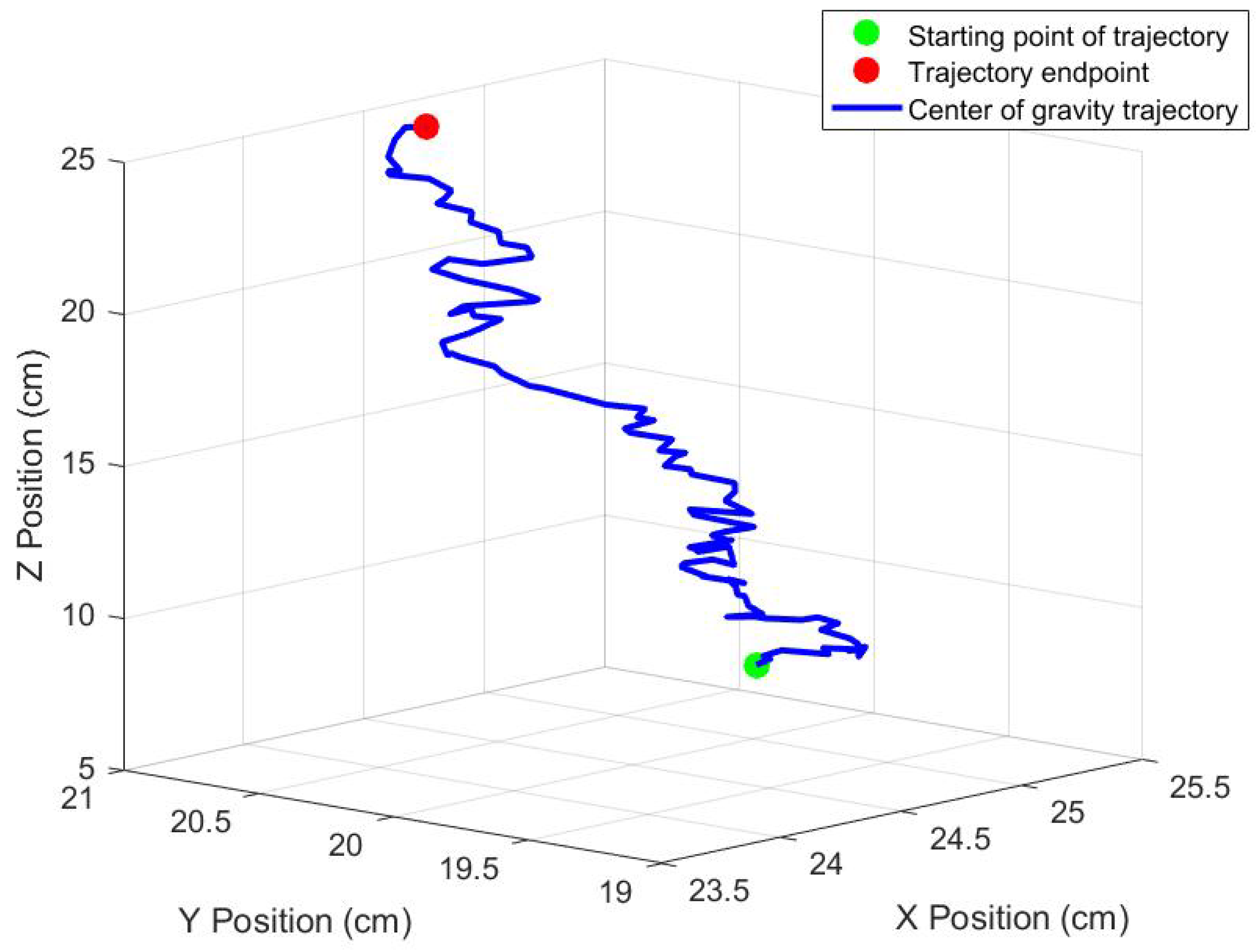
As shown in Table 1, the number of discrete elements in the simulation system is adaptively determined by the volume of the meat cuts to achieve an optimal balance between model fidelity and computational efficiency. Figure 1 illustrates the simulated trajectory of the CoG generated using the motion model parameters specified in Table 1. This trajectory faithfully reflects the dynamic deformation characteristics of the meat cuts during the grasping process and serves as a reliable ground truth for subsequent algorithm validation.

An improved Bayesian filtering algorithm is employed, augmented with a relative entropy evaluation—specifically, the Kullback–Leibler Divergence (KLD)—between the predicted values and the reference values. By dynamically adjusting the covariance matrix parameters within the likelihood function based on the real-time KLD calculation, the algorithm achieves enhanced adaptivity and predictive robustness. The key parameter settings of the algorithm, including the process noise covariance, measurement noise covariance, and adaptive adjustment coefficient, are provided in

Table 2. Algorithm parameter settings.

Parameter	Symbol	Parameter Values
Tracking duration	T	5 s
Sampling period	$\tau$	0.05 s
Target number	$\vartheta$	1
Target survival time	g	1
Initial speed	$\phi$	$T+1$
Covariance matrix	R	[3,3,1]
Error compensation weight	$\gamma$	$0.7$

. These parameters are systematically optimized to ensure algorithmic stability across diverse operating conditions.

4.2. Performance Index

4.2.1. Optimal Sub-Pattern Assignment (OSPA) Distance

The Optimal Sub-Pattern Assignment (OSPA) distance is adopted to quantify the discrepancies between target sets, particularly considering uncertainties in target positions, cardinalities, and associations. It evaluates the quality of multi-target tracking by optimally matching elements of the target sets and computing the corresponding distances. The definition of OSPA is given as follows:

$$\mathrm{OSPA}(G_{\mathrm{pre}},G_{\mathrm{ref}})={\left[{\displaystyle \frac{1}{|G_{\mathrm{pre}}|}}\sum _{i=1}^{|G_{\mathrm{pre}}|}d{(x_i,G_{\mathrm{ref}})}^p+{\displaystyle \frac{1}{|G_{\mathrm{ref}}|}}\sum _{i=1}^{|G_{\mathrm{ref}}|}d{(z_i,G_{\mathrm{pre}})}^p\right]}^{1/p}\times 100\%.$$

(36)

In the above formula, $G_{pre}$ and $G_{ref}$ represent the predicted set and the true set, respectively, while $d(x_i,G_{ref})$ and $d(z_i,G_{pre})$ represent the target position error and target cardinality error calculated using the Euclidean distance. The parameter p is used to control the sensitivity to errors, and is set here to $p=2$; $|G_{pre}|$ and $|G_{ref}|$ represent the sizes of the predicted set and the true set, respectively.

4.2.2. Average Tracking Consistency Deviation (ATCD)

The ATCD metric is employed to evaluate the accuracy and consistency of the algorithm in predicting target states across multiple time steps. It can be expressed as

$$\mathrm{ATCD}={\displaystyle \frac{1}{\vartheta }}\sum _{i=1}^1{\displaystyle \frac{1}{\Delta \tau }}\sum _{t=1}^{\Delta \tau }d(x_t,{\widehat{x}}_t)\times 100\%,$$

(37)

where $\vartheta$ represents the number of predicted targets, $\Delta \tau$ denotes the specified time step interval, and $d(x_t,{\widehat{x}}_t)$ is the deviation between the true position $x_t$ and the predicted position ${\widehat{x}}_t$ at time t. A low ATCD value indicates better consistency and stability of the target tracking, where the algorithm maintains accurate predictions with minimal trajectory deviation. In contrast, a high ATCD value reflects significant fluctuations, suggesting poor consistency and possible target drift.

4.3. Simulation Experiments

4.3.1. Simulation Experiments for the Meat Cut Dynamics Model

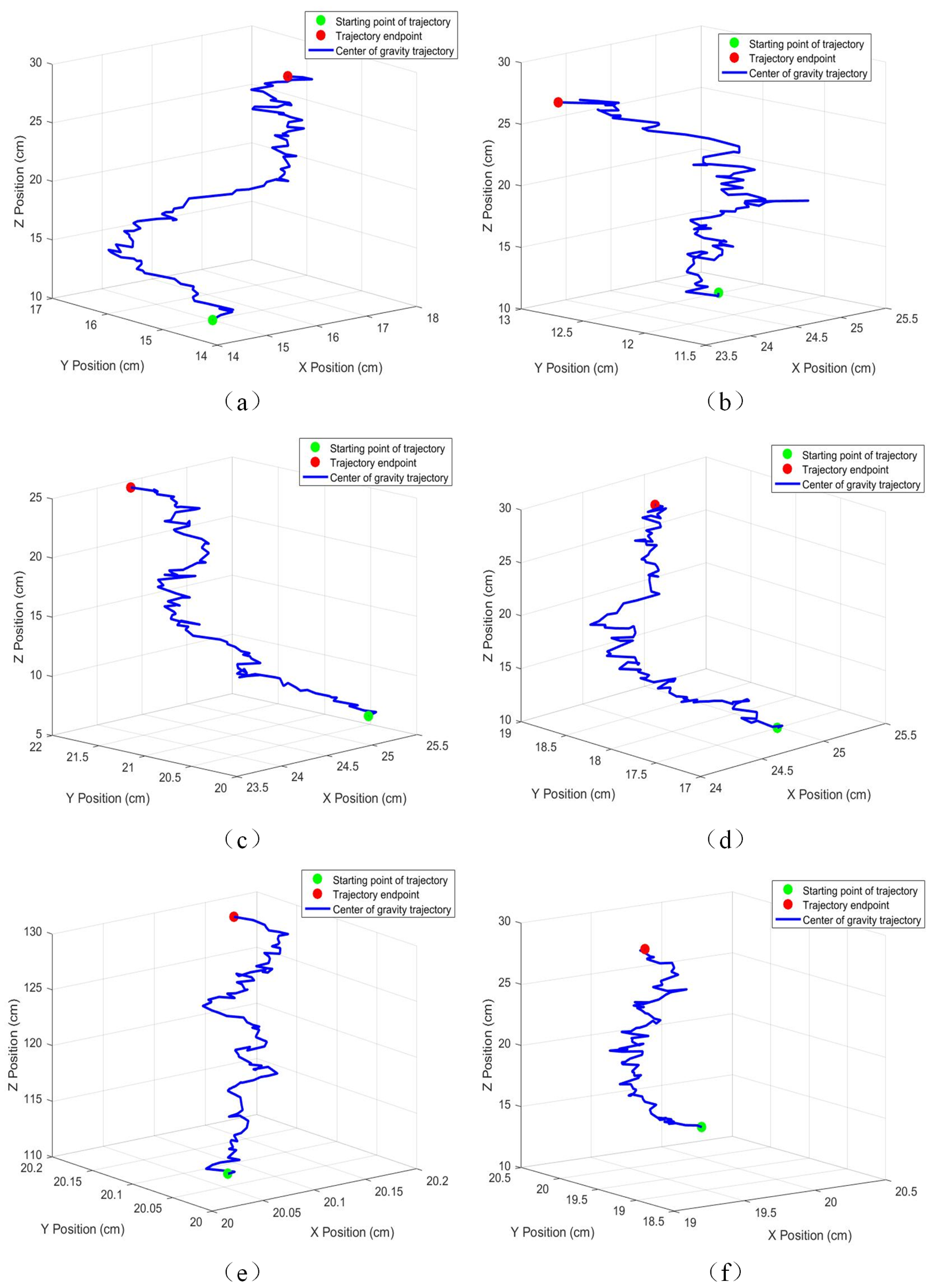
To validate the stability of the model, 50 simulation tests were conducted. By varying the volume parameter of the meat cuts ($V=0.02{\mathrm{m}}^3\mathrm{to}0.045{\mathrm{m}}^3$), the model’s performance under diverse operating conditions was systematically evaluated. Figure 2 shows the simulation results under representative conditions, with the corresponding parameter configurations detailed in

Table 3. Algorithm parameter settings.

Trajectory	Volume (m3)	Density Perturbations	Initial (cm)	Endpoint (cm)
Track (1)	0.02	1.27 $\times {10}^{-10}$	[15.01,14.99,9.98]	[17.65,16.03,27.23]
Track (2)	0.025	8.30 $\times {10}^{-10}$	[25.02,12.51,9.93]	[23.55,12.73,27.24]
Track (3)	0.03	2.11 $\times {10}^{-10}$	[24.97,20.01,7.49]	[24.28,21.91,24.74]
Track (4)	0.035	1.66 $\times {10}^{-10}$	[24.99,17.50,10.01]	[25.02,18.91,27.25]
Track (5)	0.04	3.74 $\times {10}^{-10}$	[20.71,21.32,11.23]	[20.15,20.16,28.98]
Track (6)	0.045	1.10 $\times {10}^{-10}$	[20.03,19.95,12.49]	[19.20,19.25,29.74]

.

The density disturbance parameter in Table 3 represents the effect of introducing a density perturbation term $\delta {\rho }_x$ to the discrete elements of the meat cuts. Results indicate that this term enhances the realism of the model without introducing additional interference. Across all 50 simulation tests, the motion model effectively captured the center-of-gravity (CoG) trajectory during the grasping process, with no trajectory drift observed. Furthermore, the model demonstrated strong generalization ability across meat cuts of different volumes.

The density disturbance parameter in Table 3 represents the impact of adding a density disturbance term $\delta \rho \left(\mathbf{x}\right)$ to the discrete units of segmented meat on the initial parameters. The results show that the introduction of the density disturbance term enhances the model’s realism without introducing new interference. The simulation results demonstrate that the developed motion model effectively captures the center-of-gravity trajectory of segmented livestock meat during the grasping process, with no trajectory drift observed in the fifty simulation tests. Additionally, the model developed in this study exhibits strong generalization capabilities for segmented meat of varying volumes.

4.3.2. Trajectory Prediction Experiments

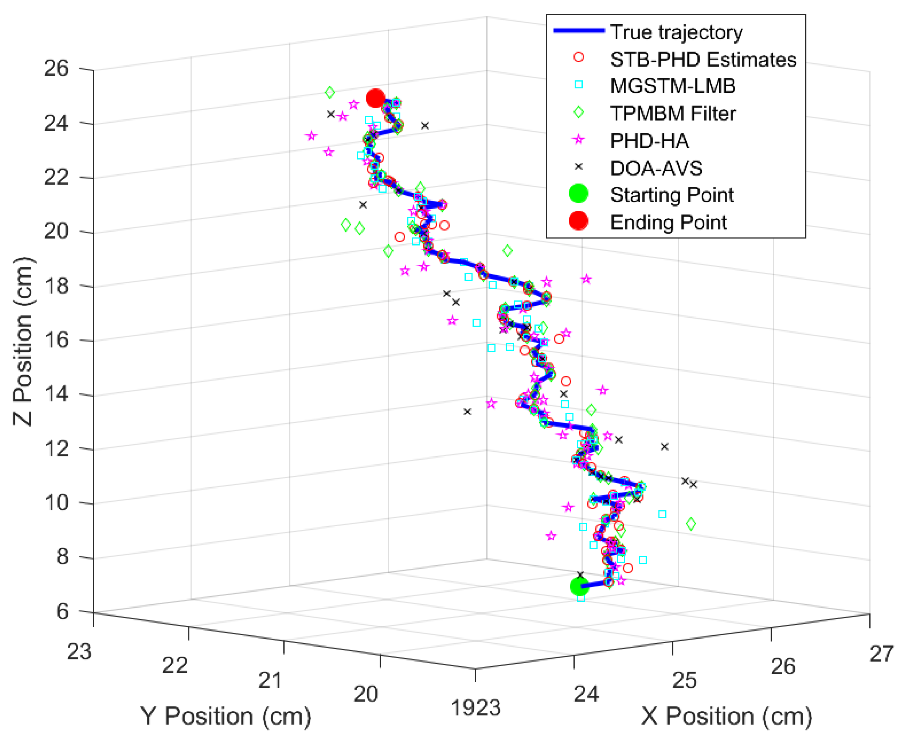
To further evaluate the effectiveness and superiority of the proposed STB-PHD algorithm, comparative experiments were conducted against four mainstream multi-object tracking algorithms: MGSTM-LMB [29], the TPMBM Filter [30], PHD-HA [31], and DOA-AVS [32]. Figure 3 presents the tracking results of the five algorithms on the same ground-truth CoG trajectory. As shown in Figure 3, the estimates from the proposed STB-PHD algorithm (red circles) align closely with the ground-truth trajectory (blue solid line), exhibiting excellent fidelity. STB-PHD maintained robust tracking performance, particularly in regions with sharp turns, whereas the other algorithms suffered from issues such as scattered estimates, drift, and even track loss.

As shown in Figure 4, analysis of comparative experimental results reveals significant differences in trajectory prediction performance among algorithms for flexible meat grasping. The STB-PHD algorithm (orange curve) demonstrated optimal performance, maintaining positional deviations consistently within 0.5 cm, validating the effectiveness of its adaptive error compensation mechanism. The newly introduced Starting Point method (black curve) achieved intermediate performance, significantly outperforming traditional multi-object tracking algorithms but slightly underperforming STB-PHD. MGSTM-LMB (purple) and TPMBM Filter (green) exhibited substantial fluctuations during the mid-to-late grasping phases, with positional deviations exceeding 1.2 cm, while PHD-HA (light blue) performed the worst. Experimental results demonstrate that the STB-PHD framework, which integrates physical dynamics models with probabilistic filtering, effectively addresses challenges posed by flexible body deformation, providing a reliable solution for stable robotic grasping.

In

Table 4. Average performance metrics comparison of algorithms (Optimal: Bold).

Methods	OSPA (%)	ATCD (%)	$\overline{\mathit{d}}$ (cm)	Comp. Time (s)	TC Time (s)
MGSTM-LMB	9.17	11.73	0.46	3.2512	6.54
TPMBM Filter	13.25	8.86	0.57	2.8273	7.25
PHD-HA	15.07	19.51	0.81	1.9688	7.62
DOA-AVS	21.33	17.46	1.11	2.5271	7.71
STB-PHD	4.82	8.33	0.19	2.1185	6.15

, Comp.Time denotes the algorithm computation time, while TC Time represents the task completion time, i.e., the total duration from the initial grasping point to the successful object grasp. The STB-PHD algorithm significantly outperforms other comparison algorithms in trajectory prediction accuracy, achieving optimal results across all three metrics: OSPA (4.82%), ATCD (8.33%), and TC time (6.15 s). Specifically, while the algorithm from MGSTM demonstrated satisfactory track maintenance performance (OSPA = 9.17%), it exhibited considerable trajectory drift (ATCD = 11.73%). The algorithm from TPMBM performed adequately in controlling trajectory drift (ATCD = 8.86%) but suffered from a high track loss rate (OSPA = 13.25%). In contrast, the algorithms from PHD-HA (OSPA = 15.07%, ATCD = 19.51%) and DOA-AVS (OSPA = 21.33%, ATCD = 17.46%) showed suboptimal performance across both critical metrics. Furthermore, the average estimation error of the STB-PHD algorithm was only 0.19 cm, substantially lower than other methods, demonstrating its superior capability in accurately reconstructing the target’s true motion trajectory. Regarding computational efficiency, the execution time for STB-PHD was 2.1185 s, which outperformed MGSTM, TPMBM, and DOA-AVS, though marginally slower than PHD-HA. This slight increase in computational overhead is acceptable given the substantial improvement in accuracy. Therefore, these results conclusively demonstrate that STB-PHD significantly enhances trajectory estimation accuracy while maintaining computational efficiency, establishing its notable advantages in both prediction precision and stability.

The quantitative results in Table 4 further substantiate these observations. It is essential to emphasize that the fundamental reason for the significant performance improvement observed in the experiments stems from the fact that the selected comparative algorithms were all designed for general-purpose multi-object tracking scenarios. Their underlying models fail to account for the intrinsic dynamics induced by the physical deformation of deformable objects. When these generic algorithms are directly applied to the highly nonlinear and non-rigid problem investigated in this study, their performance degradation is anticipated. This outcome underscores the necessity of developing specialized physics-informed prediction algorithms for such specific industrial applications, and consequently validates the effectiveness of the proposed methodology.

4.3.3. Ablation Experiments

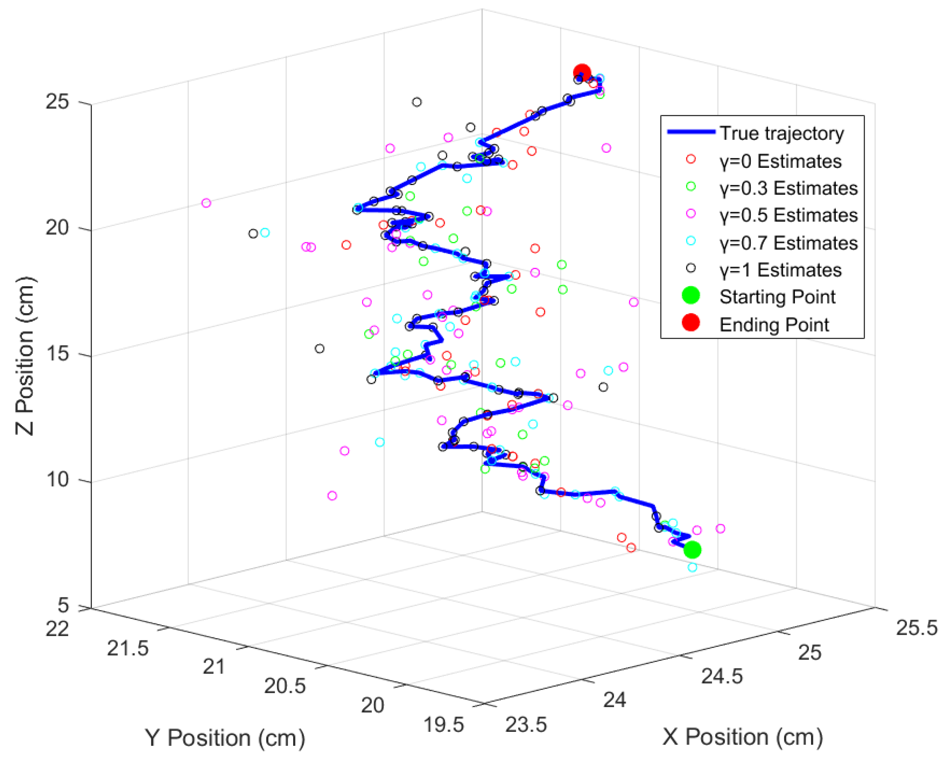
To validate the effectiveness of the core innovation in this paper—the adaptive error compensation mechanism—an ablation study was conducted. We systematically evaluated the impact of this mechanism on the algorithm’s performance by adjusting the error compensation weight $\gamma$, which controls the degree of its intervention (where $\gamma =0$ corresponds to completely disabling the mechanism). The results of this experiment are presented in Figure 5 and Table 4.

The quantitative data in

Table 5. Average performance metrics comparison of algorithms.

$\mathit{\gamma }$	OSPA (%)	ATCD (%)	$\overline{\mathit{d}}$ (cm)	Comp. Time (s)
0	14.46	19.41	0.35	1.8337
0.3	11.37	14.66	0.28	1.9131
0.5	7.22	13.18	0.22	1.9167
0.7	6.49	9.15	0.16	2.0128
1	12.16	6.84	0.12	2.1160

clearly reveal the critical role of the error compensation weight $\gamma$. When the compensation mechanism was disabled ($\gamma =0$), the algorithm exhibited its poorest performance (OSPA = 14.46%). As the value of $\gamma$ increased, the algorithm began to fuse the reference information from the dynamics model, resulting in significant improvements in both trajectory prediction accuracy (OSPA) and stability (ATCD). However, when $\gamma =1$, which signifies complete reliance on the dynamics model for strong correction, trajectory integrity (OSPA) deteriorated, although trajectory stability (ATCD) reached its optimum. This suggests that an over-reliance on the model can render the filter insensitive to actual random perturbations, leading it to erroneously “correct” away valid trajectory points.

An optimal balance between prediction accuracy, drift suppression, and computational efficiency was achieved when $\gamma =0.7$. Thus, it was selected as the optimal parameter configuration in this paper. This experiment strongly demonstrates that the proposed adaptive error compensation mechanism is a core element for enhancing the algorithm’s performance.

4.4. Application Testing

To validate the effectiveness and robustness of the proposed STB-PHD algorithm in a real-world physical environment, a series of application tests were conducted on the industrial-grade meat processing robotic platform shown in Figure 6. These tests aimed to examine the feasibility of transitioning the algorithm from simulation to practical implementation. The entire experimental platform (Figure 6) primarily consists of a conveyor belt, a robotic system (with its control cabinet shown), a weighing module, and a vision acquisition system. The vision acquisition system, positioned above the conveyor belt, comprises an RGB camera and a depth camera. These are utilized to acquire the color texture and 3D point cloud information of the meat cuts, respectively, providing initial target state data for the grasping task. The robot’s end-effector is equipped with a self-developed compliant gripper, as illustrated in Figure 6. This gripper is specifically designed for the enveloping grasp of irregular deformable objects. It incorporates a six-axis force/torque sensor internally, which provides real-time feedback of force and torque data from contact with the meat cuts during the grasping process. These data serve as the key input for the STB-PHD prediction model proposed in this study.

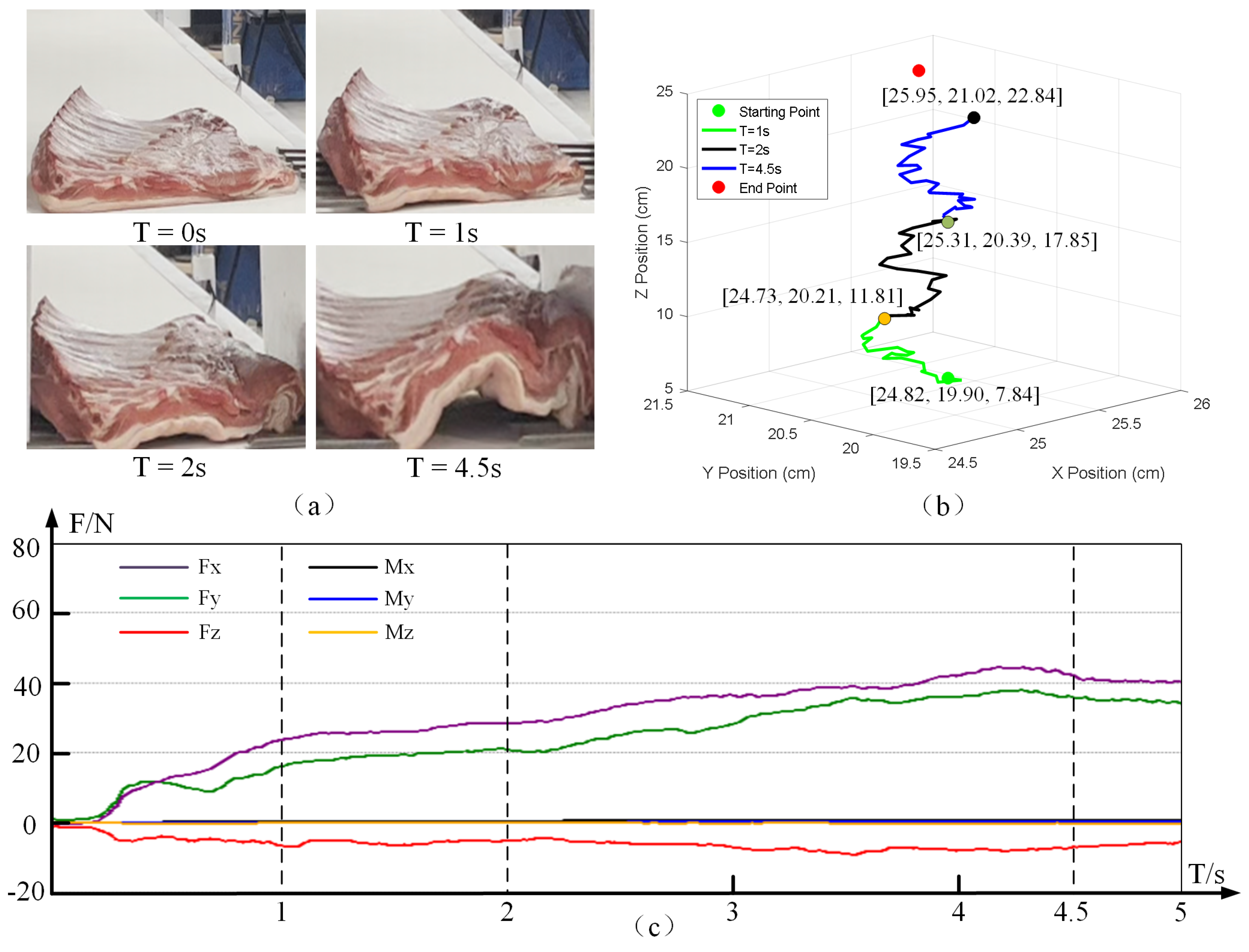
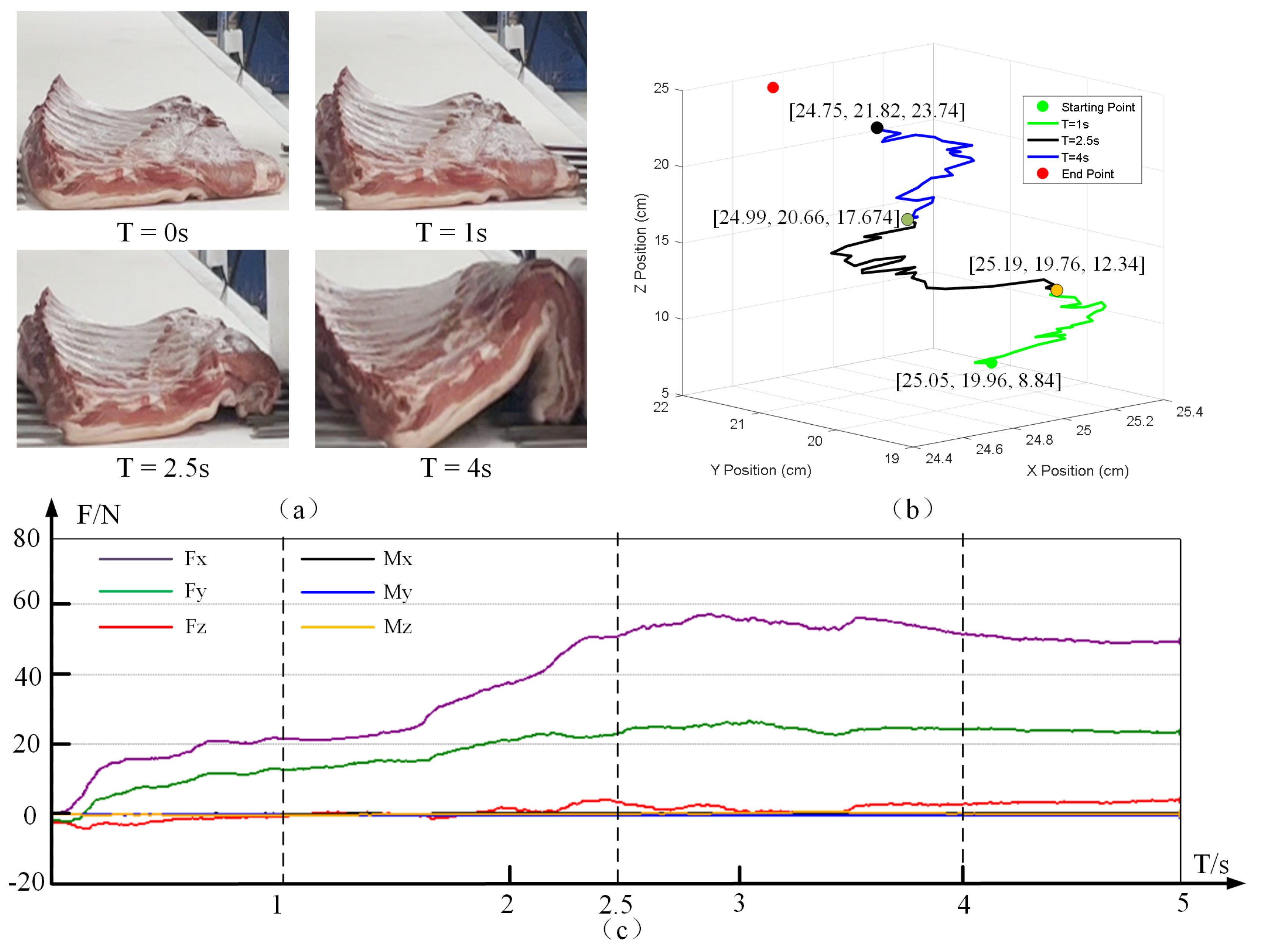
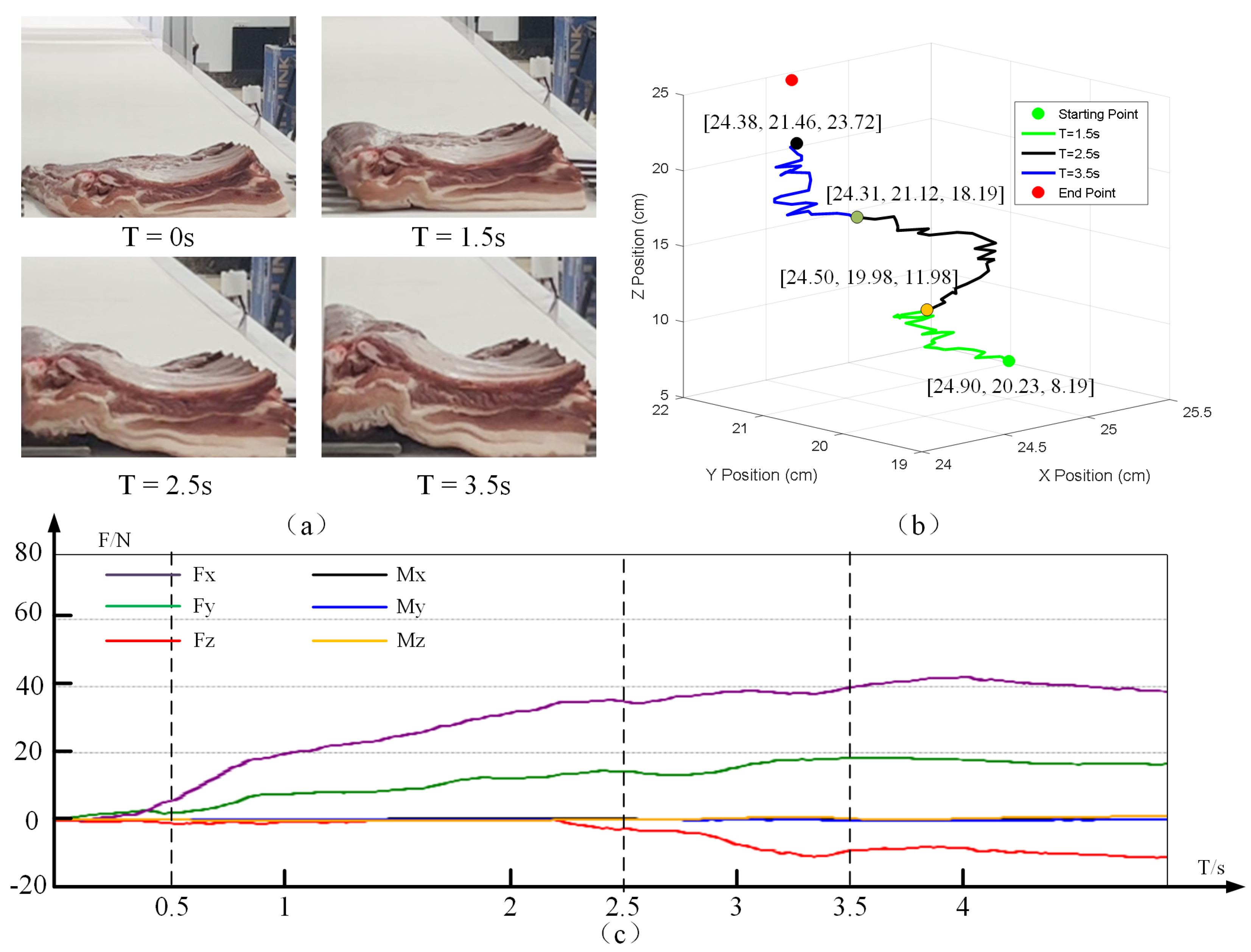
The experimental setup was as follows. First, meat cuts from carcasses were selected as test samples, varying in both specifications and and mass. The real-time force feedback data from the gripper served as the model input. To validate the model’s stability in response to unexpected situations, scenarios with force feedback data loss were simulated during the experiments. Subsequently, multiple trials were conducted under different experimental conditions to calculate the average error. Some of the test results are shown in Figure 7, Figure 8 and Figure 9, and the experimental conditions are detailed in

Table 6. Experimental conditions for application testing.

Experimental	Quality (kg)	Data Loss Rate (%)
Group 1	5.25	5
Group 1	5.42	10
Group 1	5.74	15

.

Taking Figure 7 as an example, we analyze the different states of the meat chunk at four randomly selected moments during the grasping process. Figure 7a illustrates the degree of deformation occurring in the gripper during the grasping process at different moments. Figure 7b presents the trajectory prediction results of the STB-PHD algorithm at these four moments, with the center of gravity coordinates at the current moment annotated. Figure 7c shows the points marked by dashed lines on the force feedback data curve corresponding to these moments.

The experiments demonstrate that the STB-PHD algorithm can handle test samples of varying specifications and mass and that it maintains stable predictions even in the face of partial data loss. To evaluate the influence of the meat cuts’ mass and the data loss rate on the algorithm’s performance, this study conducted further experiments using the control-of-variables method. The experimental variable settings and their corresponding performance metrics are detailed in

Table 7. Average performance metrics comparison of algorithms.

	Quality (kg)	Data Loss Rate (%)	OSPA (%)	ATCD (%)	Mean Error (cm)	Comp. Time (s)	TC Time (s)
Group 1	5.25	5	5.42	7.23	0.15	1.9157	6.15
		10	7.15	6.48	0.17	1.9453
		15	8.32	6.55	0.14	1.8819
Group 2	5.42	5	6.46	8.49	0.21	2.0849	6.17
		10	7.54	7.43	0.22	2.1127
		15	11.48	8.64	0.17	2.2582
Group 3	5.74	5	4.19	7.46	0.24	2.5094	6.16
		10	9.73	9.11	0.21	2.4451
		15	11.61	6.26	0.19	2.5218

.

Analysis of the data in Table 7 indicates that the data loss rate significantly impacts the OSPA metric and the mean error, while its effects on the ATCD metric, computation time, and TC Time are less pronounced. As the rate of force feedback data loss increases, the STB-PHD algorithm loses a necessary condition for its CoG prediction. Although the algorithm can compensate for the loss of predicted track points by leveraging historical information, higher data loss rates exceed its compensation capacity. Regarding the average error, an increase in the data loss rate within a certain range leads to a higher average error. This can be interpreted as the compensation process based on historical data, introducing larger discrepancies between the predicted results and the actual CoG coordinates. However, when the data loss rate surpasses a certain threshold, it exceeds the algorithm’s ability to compensate, resulting in an excessive loss of predicted track points. As a result, this paradoxically reduces the calculated average error of the trajectory.

An increase in the mass of the meat cuts has a relatively minor impact on the OSPA and ATCD metrics but a more significant effect on the average error and computation time. Specifically, the degree of drift and the incidence of track loss in the predicted CoG trajectory show little correlation with the mass of the meat cuts. Considering that the CoG coordinates are calculated as a weighted average of the mass and position of the object’s minimal elements, the number of discrete elements increases with the mass. Therefore, the change in computation time can be described as having a linear relationship with the change in the meat cuts’ mass. Concurrently, the increase in discrete elements introduces greater uncertainty into the CoG calculation, ultimately leading to a higher average error.

To further validate the practical effectiveness of the proposed framework, additional experiments were conducted to assess the gripper’s real-time posture adjustment and the trajectory correction of the center of gravity (CoG) during grasping.

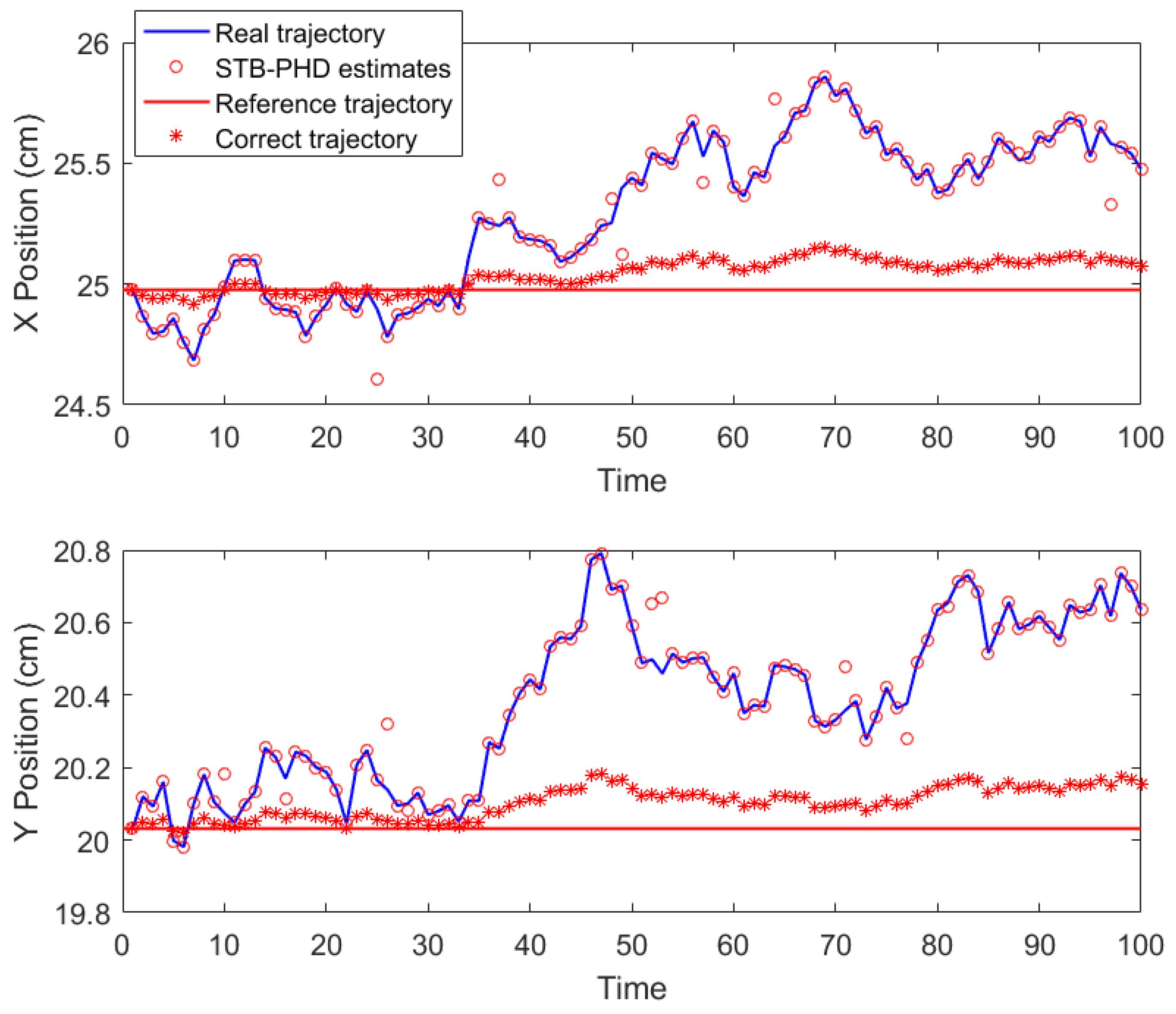
Figure 10 presents the corresponding CoG trajectory results. The blue solid line represents the measured CoG motion, the red circles denote the CoG trajectory predicted by the proposed STB-PHD algorithm, the red dashed line indicates the theoretical reference trajectory, and the red stars mark the corrected CoG positions after compensation. Quantitative analysis shows that the proposed real-time posture adjustment strategy effectively corrects asymmetric CoG drift. These results confirm that integrating CoG prediction with adaptive posture control can significantly enhance the stability and precision of robotic grasping for deformable objects.

5. Conclusions

This study addresses the dynamic instability arising from asymmetric mass distribution during the automated grasping of deformable objects such as meat cuts. A comprehensive CoG trajectory prediction framework was developed by integrating physics-based dynamic modeling with an adaptive STB-PHD filter. The proposed algorithm incorporates a historical error feedback mechanism and dynamically adjusts the filter weight $\gamma$, while an error-compensated covariance matrix further corrects prediction results. This dual-optimization strategy effectively mitigates errors caused by asymmetric perturbations and enhances robustness. Extensive experiments on both simulations and industrial robotic platforms confirm that the proposed method substantially improves prediction accuracy, stability, and consistency compared with conventional algorithms.

Challenges remain when directly applying the research findings to large-scale flexible materials such as pork cuts, including mesh distortion and parameter uncertainty under large deformations. In addition, the current framework assumes prior knowledge of the average density and volume of the meat cuts, which limits the adaptability of the method to unknown or highly variable deformable objects. Future work will focus on improving the model’s generalization capability and computational efficiency by introducing online estimation of physical parameters, hybrid modeling combining physics-based and data-driven approaches, and mesh-free dynamic representations. In addition to its practical contribution to intelligent meat processing, this study highlights the significance of explicitly modeling symmetry-breaking and asymmetric CoG deviations in robotic manipulation, offering new insights and a generalizable pathway for handling complex deformable objects.

References

1. Dey, S.; Ajay, A.; Kumar, Y.; Bhardwaj, S.; Lacerda, L.G.; Tarafdar, A. Pork processing, its quality, and safety. In Commercial Pig Farming; Academic Press: Cambridge, MA, USA, 2025; pp. 361–381. [Google Scholar]
2. Wang, M.; Li, X. Application of artificial intelligence techniques in meat processing: A review. J. Food Process Eng. 2024, 47, e14590. [Google Scholar] [CrossRef]
3. Du, G.; Wang, K.; Lian, S.; Zhao, K. Vision-based robotic grasping from object localization, object pose estimation to grasp estimation for parallel grippers: A review. Artif. Intell. Rev. 2021, 54, 1677–1734. [Google Scholar] [CrossRef]
4. Tian, H.; Song, K.; Li, S.; Ma, S.; Xu, J.; Yan, Y. Data-driven robotic visual grasping detection for unknown objects: A problem-oriented review. Expert Syst. Appl. 2023, 211, 118624. [Google Scholar] [CrossRef]
5. Zhang, J.; Li, M.; Feng, Y.; Yang, C. Robotic grasp detection based on image processing and random forest. Expert Syst. Appl. 2020, 79, 2427–2446. [Google Scholar] [CrossRef]
6. Liu, S.; Wang, F.; Liu, Z. A two-finger soft-robotic gripper with enveloping and pinching grasping modes. IEEE-ASME Trans. Mechatron. 2020, 26, 146–155. [Google Scholar] [CrossRef]
7. Yan, X.; Hsu, J.; Khansari, M.; Bai, Y.; Pathak, A.; Gupta, A. Learning 6-dof grasping interaction via deep geometry-aware 3d representations. IEEE 2018, 3766–3773. [Google Scholar] [CrossRef]
8. Cao, H.; Chen, G.; Li, Z. Efficient grasp detection network with Gaussian-based grasp representation for robotic manipulation. IEEE-ASME Trans. Mechatron. 2022, 28, 1384–1394. [Google Scholar] [CrossRef]
9. Zhang, Y.; Xie, L.; Li, Y.; Li, Y. A neural learning approach for simultaneous object detection and grasp detection in cluttered scenes. Front. Comput. Neurosci. 2023, 17, 1110889. [Google Scholar] [CrossRef]
10. Yazid, Y.; Guerrero-González, A.; El Oualkadi, A.; Arioua, M. Deep Learning-Empowered Robot Vision for Efficient Robotic Grasp Detection and Defect Elimination in Industry 4.0. Eng. Proc. 2023, 58, 63. [Google Scholar]
11. Zhang, Z.; Zhou, J.; Yi, B.; Zhang, B.; Wang, K. A flexible swallowing gripper for harvesting apples and its grasping force sensing model. Comput. Electron. Agric. 2023, 204, 107489. [Google Scholar] [CrossRef]
12. Vo, B.T.; Vo, B.N. Labeled random finite sets and multi-object conjugate priors. IEEE Trans. Signal Process. 2013, 61, 3460–3475. [Google Scholar] [CrossRef]
13. Vo, B.N.; Vo, B.T.; Nguyen, T.T.D.; Shim, C. An overview of multi-object estimation via labeled random finite set. IEEE Trans. Signal Process. 2024, 72, 4888–4917. [Google Scholar] [CrossRef]
14. Kropfreiter, T.; Meyer, F.; Hlawatsch, F. An efficient labeled/unlabeled random finite set algorithm for multiobject tracking. IEEE Trans. Aerosp. Electron. Syst. 2022, 58, 5256–5275. [Google Scholar] [CrossRef]
15. Ishtiaq, N.; Gostar, A.K.; Bab-Hadiashar, A.; Hoseinnezhad, R. Interaction-aware labeled multi-bernoulli filter. IEEE Trans. Intell. Transp. Syst. 2023, 24, 11668–11681. [Google Scholar] [CrossRef]
16. Yang, J.; Liu, W. A Two-Stage Feature Point Detection and Marking Approach Based on the Labeled Multi-Bernoulli Filter. Sensors 2022, 22, 5083. [Google Scholar] [CrossRef]
17. Wang, K.; Zhang, Q.; Hu, X. Label GM-PHD Filter Based on Threshold Separation Clustering. Sensors 2021, 22, 70. [Google Scholar] [CrossRef]
18. Zhao, J.; Zhan, R.; Liu, S.; Bo, L.; Zhuang, Z.; Li, K. Sequential joint state estimation and track extraction algorithm based on improved backward smoothing. Remote Sens. 2023, 15, 5369. [Google Scholar] [CrossRef]
19. LeGrand, K.A.; Ferrari, S. Split happens! Imprecise and negative information in Gaussian mixture random finite set filtering. arXiv 2022, arXiv:2207.11356. [Google Scholar]
20. Van Ma, L.; Nguyen, T.T.D.; Shim, C.; Kim, D.Y.; Ha, N.; Jeon, M. Visual multi-object tracking with re-identification and occlusion handling using labeled random finite sets. Pattern Recognit. 2024, 156, 110785. [Google Scholar] [CrossRef]
21. Liu, Z.; Zhou, C.; Luo, J. Adaptive marginal multi-target Bayes filter without need for clutter density for object detection and tracking. Appl. Sci. 2023, 13, 11053. [Google Scholar] [CrossRef]
22. Liu, J.; Bai, L.; Xia, Y.; Huang, T.; Zhu, B.; Han, Q. GNN-PMB: A simple but effective online 3D multi-object tracker without bells and whistles. IEEE Trans. Intell. Veh. 2022, 8, 1176–1189. [Google Scholar] [CrossRef]
23. Zhang, Y.; Shi, Z.; Ji, H.; Su, Z. Online multi-target intelligent tracking using a deep long-short term memory network. Chin. J. Aeronaut. 2023, 36, 313–329. [Google Scholar] [CrossRef]
24. Trezza, A.; Bucci, D.J.; Varshney, P.K. Multi-sensor joint adaptive birth sampler for labeled random finite set tracking. IEEE Trans. Signal Process. 2022, 70, 1010–1025. [Google Scholar] [CrossRef]
25. Yang, J.; Xu, M.; Liu, J.; Li, F. Multiple extended target tracking based on distributed multi-sensor fusion and shape estimation. IET Radar Sonar Navig. 2023, 17, 733–747. [Google Scholar] [CrossRef]
26. Li, T. Arithmetic average density fusion—Part II: Unified derivation for unlabeled and labeled RFS fusion. IEEE Trans. Aerosp. Electron. Syst. 2024, 60, 3255–3268. [Google Scholar] [CrossRef]
27. Raissi, M.; Perdikaris, P.; Karniadakis, G.E. Physics-informed neural networks: A deep learning framework for solving forward and inverse problems involving nonlinear partial differential equations. J. Comput. Phys. 2019, 378, 686–707. [Google Scholar] [CrossRef]
28. Luo, K.; Zhao, J.; Wang, Y.; Li, J.; Wen, J.; Liang, J.; Henry, S.; Liao, S. Physics-informed neural networks for PDE problems: A comprehensive review. IEEE Trans. Aerosp. Electron. Syst. 2025, 58, 323. [Google Scholar] [CrossRef]
29. Wu, Q.; Sun, J.; Yang, B.; Shan, T.; Wang, Y. Tracking Multiple Resolvable Group Targets with Coordinated Motion via Labeled Random Finite Sets. IEEE Trans. Signal Process. 2025, 73, 1018–1033. [Google Scholar] [CrossRef]
30. Xue, X.; Wei, D.; Huang, S. A novel TPMBM filter for partly resolvable multitarget tracking. IEEE Sens. J. 2024, 24, 16629–16646. [Google Scholar] [CrossRef]
31. Xiao, S.; Tao, H.; Shen, X.; Zhang, L.; Hu, M. Joint phd filter and hungarian assignment algorithm for multitarget tracking in low signal-to-noise ratio. Radioengineering 2023, 32, 287–297. [Google Scholar] [CrossRef]
32. Zhang, J.; Bao, M.; Yang, J.; Chen, Z.; Hou, H. DOA tracking algorithm based on AVS pseudo-smoothing for coherent acoustic targets. IEEE Trans. Aerosp. Electron. Syst. 2023, 59, 8175–8193. [Google Scholar] [CrossRef]
Figure 1. Simulated trajectory of the meat cut’s center of gravity.
Symmetry 17 01857 g001
Figure 2. Simulation trajectory diagram for stability testing; Figures (af) correspond to simulation trajectories for volume parameters of 0.02 m3, 0.025 m3, 0.03 m3, 0.035 m3, 0.04 m3, and 0.045 m3, respectively.
Symmetry 17 01857 g002
Figure 3. Comparison chart of prediction effect.
Symmetry 17 01857 g003
Figure 4. Trajectory experiment error.
Symmetry 17 01857 g004
Figure 5. Visualization of trajectory prediction results from the ablation study.
Symmetry 17 01857 g005
Figure 6. The meat cut grasping experimental platform and end-effector gripper.
Symmetry 17 01857 g006
Figure 7. Grasping process for a 5.25 kg pork cut with 5% force feedback data loss; (a) shows the degree of deformation at different time points, (b) presents trajectory prediction results for four time points, and (c) displays force feedback data.
Symmetry 17 01857 g007
Figure 8. Grasping process for a 5.42 kg pork cut with 10% force feedback data loss. (a) shows the degree of deformation at different time points, (b) presents trajectory prediction results for four time points, and (c) displays force feedback data.
Symmetry 17 01857 g008
Figure 9. Grasping process for a 5.74 kg pork cut with 15% force feedback data loss. (a) shows the degree of deformation at different time points, (b) presents trajectory prediction results for four time points, and (c) displays force feedback data.
Symmetry 17 01857 g009
Figure 10. Trajectory correction visualization.
Symmetry 17 01857 g010