Abstract
(1) Background: Ultra-short-term photovoltaic (PV) power prediction is crucial for optimizing grid scheduling and enhancing energy utilization efficiency. Existing prediction methods face challenges of missing data, noise interference, and insufficient accuracy. (2) Methods: This study proposes a single-step hybrid neural network model integrating Temporal Convolutional Network (TCN), Temporal Shift Transformer (TST), and Bidirectional Gated Recurrent Unit (BiGRU) to achieve high-precision 15-minute-ahead PV power prediction, with a design aligned with symmetry principles. Data preprocessing uses Variational Mode Decomposition (VMD) and random forest interpolation to suppress noise and repair missing values. A symmetric parallel dual-branch feature extraction module is built: TCN-TST extracts local dynamics and long-term dependencies, while BiGRU captures global features. This symmetric structure matches the intra-day periodic symmetry of PV power (e.g., symmetric irradiance patterns around noon) and avoids bias from single-branch models. Tensor concatenation and an adaptive attention mechanism realize feature fusion and dynamic weighted output. (3) Results: Experiments on real data from a Xinjiang PV power station, with hyperparameter optimization (BiGRU units, activation function, TCN kernels, TST parameters), show that the model outperforms comparative models in MAE and R2—e.g., the MAE is 26.53% and 18.41% lower than that of TCN and Transforme. (4) Conclusions: The proposed method achieves a balance between accuracy and computational efficiency. It provides references for PV station operation, system scheduling, and grid stability.
1. Introduction
Against the backdrop of accelerating transformation of the global energy structure, photovoltaic (PV) power generation has become a core driver in achieving the “dual carbon” goals. According to the International Renewable Energy Agency (IRENA), global PV installed capacity is expected to exceed 1.5 TW by 2025, and the inherent volatility of PV generation poses severe challenges to the secure operation of power grids. To address this, PV power prediction is classified into a four-level system based on time scale: ultra-short-term, short-term, medium-term, and long-term. Ultra-short-term prediction refers to forecasting within one hour, supporting real-time grid operation adjustment; short-term prediction covers the range from one hour to one day, serving daily management; medium-term prediction spans from one day to several weeks, providing guidance for maintenance and operation; long-term prediction focuses on trends over several months to years, offering data support for strategic market planning [1,2].
PV power prediction is a key technology for improving grid absorption capacity. Existing prediction methods can be broadly divided into three categories: physics-based, statistical, and hybrid approaches. Physics-based methods construct physical models of PV cells combined with meteorological and geographic data to simulate the generation process. These methods are mechanistically transparent but constrained by difficulties in parameter acquisition and data resolution, making it challenging to capture subtle fluctuations [3,4]. Statistical methods rely on historical data to establish input–output mapping relationships, including traditional time series models and machine learning algorithms. However, these methods are highly sensitive to noise, prone to overfitting due to the stochastic nature of PV generation, and often lack cross-site generalization capability. Hybrid methods [5,6] integrate the strengths of both approaches: physical models provide theoretical mechanisms, while statistical models compensate for data uncertainties, thereby significantly improving prediction accuracy and robustness.
In recent years, deep learning has shown great potential in PV power prediction. For temporal modeling, recurrent neural networks (RNNs) capture sequence dependencies through recurrent structures but suffer from gradient vanishing, limiting their ability to model long-term dependencies. Long Short-Term Memory (LSTM) networks effectively mitigate this issue via gating mechanisms, achieving superior performance in complex nonlinear mapping tasks [7]. Bidirectional LSTM (BiLSTM) further enhances feature extraction by modeling both forward and backward temporal dependencies. However, single models often have inherent limitations, leading to unsatisfactory performance. Models such as Generative Adversarial Networks (GANs) and feedforward neural networks have been explored, but their effectiveness remains constrained. To overcome this, ensemble prediction methods have become a research hotspot, leveraging multiple models’ advantages to improve forecasting accuracy [8,9,10].
Wang et al. proposed a model combining Gaussian Mixture Models and Variational Mode Decomposition (VMD) to effectively address the strong randomness and volatility of PV power generation, achieving robust performance against weather variability in prediction accuracy [11]. Nevertheless, VMD has limitations in handling missing and abnormal PV data, especially when continuous segments of data are missing. To this end, this study introduces a random forest-based imputation method on top of VMD to leverage feature correlations with missing data for more accurate completion. Du Plessis A.A. et al. proposed a joint model of feedforward neural networks and LSTM, demonstrating lightweight advantages by optimizing the workload of multiple low-level predictors [12]. Although these approaches achieve strong results across diverse data scenarios, their flexibility and ability to handle complex nonlinear relationships remain insufficient. Therefore, this paper proposes a joint modeling approach based on TCN and BiGRU to enhance adaptability to data complexity. Huang et al. developed a model combining LSTM with attention mechanisms [13], achieving notable improvements in spatiotemporal feature extraction and optimization, and reporting lower prediction errors on multiple datasets. Despite these advantages in prediction accuracy, challenges in real-time forecasting and computational efficiency persist. To address this, we introduce a Temporal Shift Transformer (TST) module into the network structure to reduce redundant computation and improve efficiency, ensuring high-precision forecasting under efficient operation.
At present, PV power prediction models generally focus on the spatiotemporal characteristics of weather and PV output, and while deep learning methods have achieved remarkable progress, issues related to prediction accuracy, computational efficiency, and generalization still leave room for improvement [14,15]. Building on the above research, this paper proposes an innovative parallel hybrid model named TCN-TST-BiGRU. The core advantage of this model lies in its symmetric parallel architecture, which synergistically leverages the strengths of different models. Specifically, one branch utilizes TCN to capture local dynamic features of time series, while combining TST to efficiently model long-term dependencies. The introduction of TST is one of the key innovations in this paper. Its temporal shift module achieves information exchange between adjacent time steps at minimal computational cost through feature movement in the temporal dimension, effectively capturing the rapid fluctuations of photovoltaic power. Meanwhile, its built-in multi-head self-attention mechanism establishes relationships between any two time points in the sequence, perfectly capturing long-term patterns such as the daily periodicity of photovoltaic power. The other branch employs bidirectional gated recurrent units (BiGRU) to capture forward and backward contextual information from a global perspective. This dual-branch symmetric design ensures the model does not favor any single type of feature, but comprehensively understands photovoltaic power sequences from multiple dimensions including local–global and short-term–long-term perspectives, thereby significantly improving prediction accuracy and robustness.
2. Materials and Methods
2.1. Variable Mode Decomposition
PV power time-series data are influenced by factors such as solar irradiance cycles and sudden weather changes, exhibiting both seasonal trends and minute-level fluctuations. Traditional single-scale modeling methods struggle to simultaneously capture global patterns and local details. To more effectively extract multi-scale features, this study adopts Variational Mode Decomposition (VMD) to decompose the original data into several modal components with distinct frequency characteristics, where each mode corresponds to variations in the data at a specific time scale. In this way, the dynamic characteristics of time-series data across different scales can be more clearly revealed. These modal components are then used as input features for the prediction model, enabling it to fully exploit multi-scale information during training, thereby improving adaptability to PV power fluctuations and enhancing prediction accuracy [16,17].
VMD decomposes the original PV time series into K Intrinsic Mode Functions (IMFs). An IMF is defined as a function of the input signal , as shown in Equation (1):
In Equation (1), represents the amplitude with ≥ 0, while denotes the phase. The modal function is . To obtain the instantaneous frequency, Equation (2) differentiates .
Based on the Gaussian smoothness of the demodulated signal, the bandwidth is estimated, and the constraint variational problem as Formulas (3) and (4) is constructed.
In Equation (3), represents the set of K modal function components ; denotes the set of center frequencies corresponding to each mode, and ; represents the squared norm of the demodulated signal gradient; in Equation (4), is the sequence.
By introducing a quadratic penalty term and Lagrange multiplier , the problem is transformed into an unconstrained variational problem, as shown in Equation (5):
Here, denotes the generalized Lagrangian function, which ensures the completeness of signal reconstruction, while represents the second penalty term, guarantees the strictness of the constraint conditions.
In traditional VMD, the feature extraction process of time series is still prone to significant accuracy loss due to the influence of high-frequency noise. Therefore, in this study, correlation analysis is integrated with conventional VMD. To avoid over-decomposition or under-decomposition, the correlation between each component and the original sequence is calculated, and weakly correlated or uncorrelated IMFs are removed. The remaining components are then reconstructed into a denoised sequence.
To further reduce the impact of noise on feature extraction, this method eliminates irrelevant and weakly relevant components based on the correlation coefficients between each mode and the original sequence. The process for calculating the correlation coefficient is defined as follows in Equation (6):
where denotes the correlation coefficient; represents the original time series; and refers to the decomposed components. The values of can be used to assess the correlation between patterns and the original function. Typically, strongly correlated components are reconstructed while weakly correlated ones should be removed. Table 1 illustrates the correspondence between correlation coefficients and their corresponding correlations [18,19].

Table 1.
Correlation coefficients and correlations correspond to each other.
To ensure effective decomposition and accurate subsequent analysis, we carefully optimized and selected key parameters for VMD. The bandwidth constraint parameter (alpha) was set to 2000, aiming to moderately compress the bandwidth of each mode, thereby clearly distinguishing different frequency components while preventing loss of important fluctuation details due to excessive smoothing. The number of modes (K) is the most critical parameter in VMD. Through exploratory experiments, we found that when K < 7, the decomposition is insufficient, while K > 7 begins to exhibit noticeable “mode aliasing” phenomena. Therefore, we ultimately determined K = 7 as the optimal value to achieve the best balance between effective signal separation and avoiding mode aliasing. Additionally, we set the convergence tolerance (tol) to 1 × 10⁻⁷ to ensure the algorithm converges to sufficiently precise results.
After determining the decomposition parameters, we filtered out noise by calculating the correlation coefficients between each IMF component and the original sequence. To identify the optimal correlation threshold, we conducted a sensitivity analysis. Using the TCN-TST-BiGRU model architecture detailed in Section 2.2, we preprocessed the data with different thresholds and evaluated the model’s predictive performance on the validation set. The experimental results are presented in Table 2.
Table 2.
Relevance threshold sensitivity analysis.
As shown in Table 2, the model achieved the lowest average absolute error on the validation set when the threshold was set to 0.2. This indicates that the threshold strikes the optimal balance between effectively filtering high-frequency noise modes and preserving essential signal details. Therefore, this study adopts 0.2 as the correlation threshold for IMF filtering. Ultimately, the filtered effective mode components are reconstructed into denoised sequences for subsequent model training. The reconstruction equation, shown in Formula (7), is as follows:
Among them, represents the reconstructed sequence after denoising; i represents the number of satisfactory sequences; represents the correlation coefficient between the pattern and the original sequence.
Figure 1 clearly illustrates the complete workflow: from raw data input through VMD, IMF screening based on correlation coefficients, to missing value imputation using random forest.
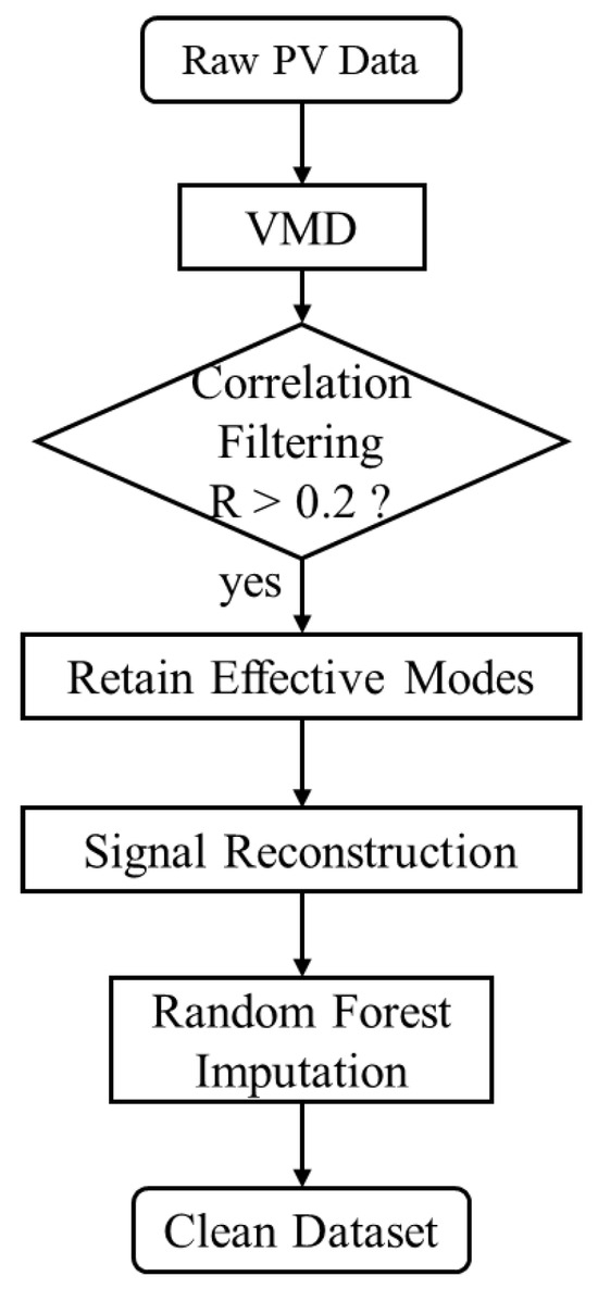
Figure 1.
Data preprocessing flowchart.
2.2. Ultra-Short-Term Photovoltaic Power Prediction Model
Unlike traditional stacked hybrid models, this paper proposes a parallel dual-channel architecture TCN-TST-BiGRU hybrid model for ultra-short-term photovoltaic power forecasting. As shown in Figure 2, the model innovatively integrates three core components: Temporal Convolutional Network (TCN), Temporal Shift Transformer (TST), and Bidirectional Gated Recurrent Unit (BiGRU). The model adopts a symmetrical parallel design to achieve balanced and comprehensive feature extraction:
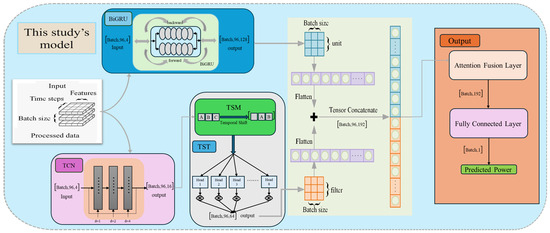
Figure 2.
Parallel dual-channel architecture TCN-TST-BiGRU hybrid model (The diagram illustrates the tensor dimensions (Tensor Dimensions) of data flow through the dual channels and the final fusion path).
Channel One (Local and Long-Term Feature Channel): In this channel, the TCN first efficiently captures local dynamic features in sequences through expansion causal convolution. The output is then fed into the TST module, which utilizes its built-in multi-head self-attention mechanism to accurately model long-term dependencies in the data, such as the daily cyclical patterns of photovoltaic power.
Channel 2 (Global Context Channel): In a parallel channel, BiGRU captures bidirectional temporal context information across the entire sequence from a global perspective through its forward and backward recurrent structures.
Both channels receive identical raw input data, with their extracted features concatenated at the model’s terminal. The resulting high-dimensional features are then fed into an attention fusion layer, which dynamically assigns weights to different features to highlight the most critical information for final predictions. This design enables the model to holistically and unbiasedly analyze time series across multiple dimensions, significantly improving prediction accuracy and robustness.
This symmetrical parallel architecture prevents the model from favoring any single type of feature extractor. The TCN-TST branch excels at capturing local details and long-term periodic patterns (such as diurnal variations), while the BiGRU branch captures global contextual dependencies. The final Attention Fusion Layer acts as a dynamic balancer, adaptively adjusting the contribution weights of the two branches based on input data characteristics. This symmetrical complementarity between local and global features is key to achieving high precision in the model.
Key architectural parameters of the model: To ensure reproducibility of this study, we detail the critical hyperparameters of each model component in Table 3 below. These parameters were determined through extensive grid search experiments on the validation set (see Section 3.2.1).
Table 3.
Table of Key Hyperparameter Settings for the Model.
2.2.1. Temporal Convolutional Network (TCN)
The TCN neural network, constructed with Dilated Causal Convolution, employs exponentially increasing dilation factors to significantly expand the receptive field while reducing network depth [20]. This design enables efficient capture of long-term temporal trends in the input data. Unlike traditional Convolutional Neural Networks (CNNs), where the receptive field grows linearly with network depth and kernel size, the dilated convolution structure of TCN allows the receptive field to expand exponentially with layer depth. Consequently, TCN can cover extremely long historical sequences with only a few layers while avoiding the vanishing gradient problem.
When the initial dilation factor is set to and the initial convolution kernel size is set to , the receptive field r of the output layer can be calculated using Equation (8):
Here, denotes the number of expanded causal convolution layers. By adjusting the values of and , the receptive field can be significantly expanded to extract long-term temporal features from input data while maintaining a relatively shallow network architecture. Given a one-dimensional input sequence X, = {,,···,}, and an dimensional convolutional filter = {, ,···, }, the expanded causal convolution result at time step t can be expressed by Equation (9) [21,22,23]:
As illustrated in Figure 3, by combining dilated causal convolution with residual stacking, the TCN is able to cover extremely long historical contexts, with its receptive field expanding exponentially. This design avoids the gradient vanishing/explosion problems that typically occur in RNNs as the number of recurrent steps increases. The residual layer not only expands the receptive field but also reduces parameter redundancy. Moreover, the identity mapping in the residual design prevents performance degradation in deep networks while saving computational resources.
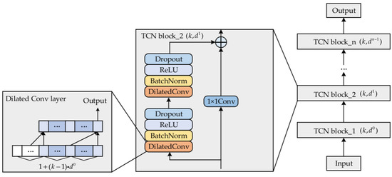
Figure 3.
TCN neural network structure.
2.2.2. Temporal Shift Transformer (TST)
To enhance the joint modeling capability of long-term dependencies and local abrupt variations, this study introduces the Temporal Shift Transformer (TST) module on top of TCN. The module integrates the Temporal Shift Module (TSM) with a multi-head self-attention mechanism, thereby significantly improving the representation of temporal dynamic features.
Specifically, the TST employs TSM to introduce cross-time-step feature interactions within the input sequence, which substantially strengthens the representation of local temporal features. For an input feature sequence X ∈ RT × d (where T denotes the number of time steps and d is the feature dimension), the TSM defines a shift offset n according to the PV data interval ∆t = 15 min:
The time-shifted sequence is fed into the multi-head self-attention mechanism. First, the input undergoes three learnable linear projection matrices , , and , which compute the query (Q), key (K), and value (V) for the i-th attention head among the h heads [24].
Next, h attention heads compute their respective output in parallel. The computational Formula (11) is as follows:
Here, is the key vector dimension of each head.
Finally, the outputs from all heads are concatenated and fused through a final linear projection matrix W^O to produce the multi-head self-attention output Z as shown in Formula (12):
The output of the STST module is a feature tensor that deeply integrates both local and global temporal dependencies. This output is then combined with features extracted from parallel BiGRU channels for final fusion.
In the TST module, we implemented eight attention heads. This configuration was determined by two key considerations: First, the eight-head setup represents a well-established and validated approach in Transformer architecture, enabling parallel learning of temporal dependencies across multiple representation subspaces to form a robust “expert committee”. Second, this configuration perfectly aligns with our 64-dimensional embedding space (64D/8 heads = 8D/head), ensuring each head can effectively learn features within sufficient dimensional subspaces. Our preliminary experiments confirmed that this setup enables the model to achieve both robustness and superior performance.
2.2.3. BiGRU Neural Network
Bidirectional Gated Recurrent Unit (BiGRU) employs reset gates and update gates to realize a gating mechanism that dynamically regulates the flow of temporal information. The reset gate controls the degree of association between the current input and the historical state, while the update gate determines whether the previous memory should be retained. This gating design significantly enhances the efficiency of modeling complex temporal dependencies [25,26,27]. The BiGRU architecture consists of an input layer, a forward GRU layer, a backward GRU layer, and an output layer. At each time step, the input layer simultaneously passes data to both the forward and backward GRU layers, allowing information to flow in two opposite directions. The output sequence is jointly determined by the two GRU networks, enabling the model to capture both past and future dependencies. The overall network structure of BiGRU is illustrated in Figure 4.
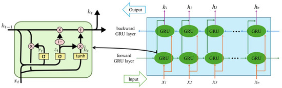
Figure 4.
BiGRU neural network structure.
2.2.4. Self-Attention Mechanism
Photovoltaic (PV) power generation is influenced by multiple coupled factors such as solar irradiance, geographical environment, and equipment conditions, exhibiting strong nonlinearity, volatility, and randomness.
Traditional time-series models (e.g., TCN, BiLSTM) face two major limitations in feature extraction, namely the reliance on sequential order and static weight allocation. To address this issue, the proposed model incorporates a self-attention mechanism in the output layer. By computing global similarity among features, self-attention enables dynamic weighting, thereby eliminating the dependence on fixed sequential order, strengthening the representation of critical features, and capturing deeper correlations. This ultimately enhances the accuracy of power prediction. The principle of the self-attention mechanism is illustrated in Figure 5.
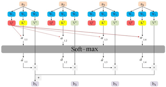
Figure 5.
Self-attention mechanism structure.
The attention calculation formula is shown in (13):
Here, a is the input vector, b is the output vector, W is the weight, Q is the query matrix, K is the key matrix, V is the value matrix, and is the dimension of the key vector.
2.3. Evaluation Indicators
For a comprehensive evaluation of the model’s performance, multiple regression metrics are employed, including MSE (Mean Squared Error), RMSE (Root Mean Squared Error), MAE (Mean Absolute Error), and R2 (coefficient of determination). Smaller values of MSE, RMSE, and MAE indicate better predictive performance, whereas a larger R2 implies superior prediction accuracy [28,29]. These metrics are computed according to Equations (14)–(17). To ensure all metrics are evaluated in their original physical units (e.g., MW), the model’s predictions must first undergo inverse normalization using parameters from the training set before calculating these metrics.
2.4. Data
This study utilizes operational monitoring data from a photovoltaic power plant in Xinjiang, covering the entire year of 2019 (sampling time: 9:00–19:00 daily, with a 15 min interval). The plant is located in a temperate continental climate zone (annual average solar radiation >1600 kWh/m2), characterized by high irradiance intensity and significant daytime fluctuations, making it a representative case for photovoltaic power prediction research. At each time point, eight feature variables are recorded, with their units and physical significance summarized in Table 4.
Table 4.
Variable table.
To ensure the rigor of the experiment and reliability of the results, we rigorously divided the entire dataset into three parts: 70% as the training set, 15% as the validation set, and 15% as the test set. The model was trained on the training set, with all hyperparameter selections (as listed in Table 3) optimized based on performance on the validation set. When constructing the model inputs, we used historical data from the past 96 time steps (representing 24 h of historical data) to predict power output for the next 15 min. The model’s generalization ability was ultimately evaluated on the test set, which the model had never encountered. This strict partitioning method effectively prevented data leakage. Before inputting data into the model, all feature variables underwent Min-Max Scaling. Importantly, the maximum and minimum values used to calculate scaling parameters were entirely derived from the training set, and the same parameters were applied to normalize both the validation and test sets.
3. Results
This study focuses on the ultra-short-term photovoltaic power prediction task in the next 15 min. The selection of model input features has a significant impact on the prediction accuracy. The correlation between each feature variable and photovoltaic power is shown in Figure 6.
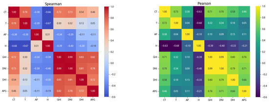
Figure 6.
Spearman correlation coefficient and Pearson correlation coefficient Figure.
In Figure 6, the Spearman correlation coefficients show that module temperature, global horizontal irradiance, direct normal irradiance, and diffuse horizontal irradiance exhibit moderate to strong correlations, with values of 0.46, 0.82, 0.78, and 0.72, respectively. Similarly, in the Pearson correlation coefficient plot, module temperature, global horizontal irradiance, direct normal irradiance, and diffuse horizontal irradiance also display moderate to strong correlations, with coefficients of 0.46, 0.76, 0.71, and 0.66, respectively. Considering the physical mechanisms of solar radiation and meteorological variables, and based on the dual analysis of both Pearson and Spearman correlation coefficients [30], module temperature (CT), global horizontal irradiance (GHI), direct normal irradiance (DNI), and diffuse horizontal irradiance (DHI) are selected as the model inputs.
3.1. VMD Combined with Random Forest to Process the Data
In this study, the Random Forest algorithm, which has demonstrated excellent performance in regression tasks, is employed to make full use of feature factors related to missing data and achieve more accurate imputation, thereby improving the overall predictive performance of the model [31]. Among the four selected variables, three are used as input features to predict the remaining one. The predicted results are compared with the true values to obtain evaluation metrics, after which the predicted values are used to fill in the deleted abnormal values and zero values. For data without anomalies, the original values are retained. A total of four experiments are conducted to impute the missing values of GHI, DNI, DHI, and APG. The evaluation metrics of these four experiments are presented in Table 5.
Table 5.
Random forest multi-feature prediction results.
Using VMD, the original sequence was decomposed into seven modes, as illustrated in Figure 7. However, the use of traditional VMD in sequence feature extraction often results in considerable accuracy loss. Therefore, after decomposing the original data into multiple IMF components, the correlation between each mode and the original sequence is calculated, and weakly correlated or uncorrelated IMFs are removed.
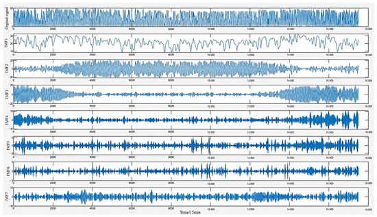
Figure 7.
Figure VMD mode components.
The remaining modes were reconstructed to form the denoised sequence, with the correlation between each mode and the original sequence shown in Figure 8. Ultimately, IMF2, IMF3, and IMF4, which exhibited correlation coefficients greater than 0.2, were retained for reconstruction. Negative values arising from the mode reconstruction were first clipped to zero and then imputed using a multi-feature Random Forest regression to ensure data consistency. The data before and after processing are shown in Table 6 and Table 7.
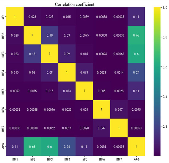
Figure 8.
Correlation thermal diagram.
Table 6.
PV data before processing.
Table 7.
Processed PV data.
3.2. Experimental Results and Analysis
3.2.1. Hyperparameter Experiments
Table 8 presents the results of hyperparameter optimization experiments for the TCN convolution kernel size and the number of GRU units, under the conditions where the TCN activation function was ReLU, the convolution kernel size was 3, the GRU activation function was Tanh, the optimizer was Adam, the batch size was 32, and the TST time shift was 1. The experimental results indicate that the proposed model achieves the best performance when the TCN convolution kernel is set to 16 and the number of GRU units is 64.
Table 8.
Experimental results of combination of TCN filter number and GRU unit number.
In a combined model, selecting the optimal parameters for each layer has a critical impact on the experimental results. Building upon the optimal parameters obtained in the previous step, when the number of TCN convolution kernels was set to 16, the influence of different kernel sizes on the experimental outcomes was further investigated. As shown in Table 9, the best performance was achieved when the kernel size was set to 3, in combination with the GRU and the attention mechanism.
Table 9.
Results of different TNC kernel sizes.
After determining the optimal parameters for the TCN layer, we proceeded to configure the GRU layer’s parameters. Table 10 presents the results under different batch sizes, GRU activation functions, and optimization methods. The best GRU activation function is SELU, the best number of samples is 32 and the best optimizer is RMSprop.
Table 10.
The effect of different sample sizes, GRU activation functions and optimizers on the results.
After determining all optimal parameters, we conducted parameter optimization for the TST layer. In the experiment, time offsets n = 0, 1, 2, and 3 (corresponding to no offset, 15 min, 30 min, and 45 min, respectively) were selected for comparison. Table 11 presents the results under different time offsets, with optimal performance achieved when the TST time offset was set to 2.
Table 11.
The effect of different time offsets on the results.
In all the hyperparameter experiments mentioned above, the training cycle (epoch) was uniformly set to 200, and L2 regularization and the early stopping strategy were adopted to prevent overfitting, ensuring the efficiency and stability of model training.
To determine the optimal model configuration, we conducted a thorough grid search on the validation set, with the best hyperparameter combinations and other experimental settings summarized in Table 3. All subsequent training and evaluation processes uniformly adopted 200 epochs, an L2 regularization coefficient of 1 × 10⁻³, and a patience of 15 for early stopping to prevent overfitting while ensuring training efficiency and stability. Throughout the training process, we closely monitored the validation set loss. We observed that L2 regularization and early stopping strategy effectively prevented model overfitting, with no significant divergence in training set or validation set losses.
3.2.2. Model Performance Evaluation Experiment
To comprehensively evaluate the model’s performance, all experiments employed K-fold cross-validation, where the dataset was divided into K mutually exclusive subsets. In each of the K iterations, K − 1 subsets were combined as the training set, and the remaining subset was used as the test set [32]. The results of each validation were reported using evaluation metrics such as MAE, R2, and MSE.
Experimental setup: All experiments were conducted on a workstation equipped with an NVIDIA RTX 3080 GPU (NVIDIA Corporation, Santa Clara, CA, USA), Intel Core i9-10900K CPU (Intel Corporation, Santa Clara, CA, USA), and 64 GB memory. The run time in Table 10 indicates the total time required for the model to complete a full inference on the entire test set when the batch size is uniformly set to 32.
To investigate the effectiveness of the proposed model, a residual distribution histogram was plotted for deeper analysis, as shown in Figure 9. It can be observed from Figure 9 that most residuals are concentrated around zero, with a relatively uniform distribution and no significant bias. This indicates that the model’s prediction errors are relatively balanced within the positive and negative ranges, and the overall predictions are unbiased. Furthermore, the residuals exhibit an approximately normal distribution, suggesting that the model effectively captures the random fluctuations in the data without apparent systematic bias, thereby providing strong evidence for its high prediction accuracy.
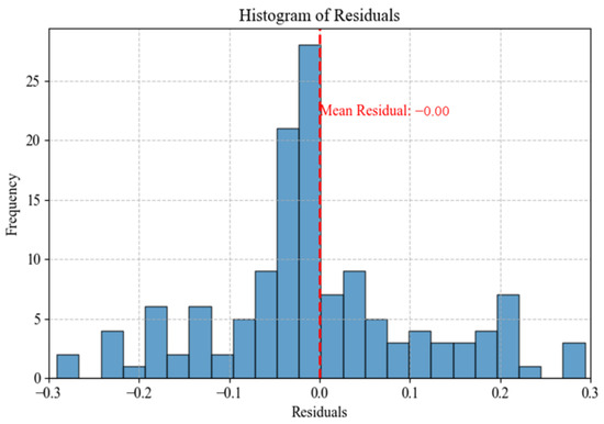
Figure 9.
Residual distribution diagram.
To validate the performance of the proposed model, 10 baseline models were selected for comparison, including single deep learning models (LSTM, GRU, BiLSTM, BiGRU), TCN-based hybrid architectures (TCN-BiLSTM, TCN-GRU, TCN-BiGRU), and TST attention-based variants (TST-LSTM, TST-GRU, TST-BiGRU). To enhance the stability and reliability of the experimental results, all models were evaluated on the same dataset using ten-fold cross-validation, and the average error metrics from the 10 experiments were reported as the final performance indicators for quantitative analysis. To ensure fairness and reliability, all single models adopted a three-layer network structure, while the hybrid models were configured with the same hyperparameter settings as the proposed model. Figure 10 presents the prediction results of each model along with a comparison of local curves. As shown in the zoomed-in plots, the prediction curve of the proposed TCN-TST-BiGRU model exhibits the closest alignment with the ground truth, demonstrating the best predictive performance.
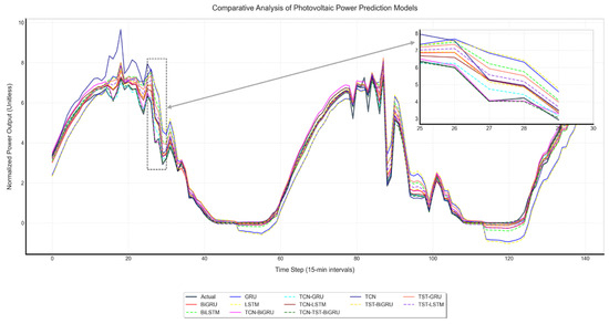
Figure 10.
Comparison of prediction results and local curves of each model.
Furthermore, to further validate the effectiveness of the proposed preprocessing method and the superiority of the TCN-TST-BiGRU model, this study conducted a series of ablation and comparison experiments. The ablation experiments included no preprocessing, random forest preprocessing alone, VMD preprocessing alone, and a TCN-BiGRU model with the TST module removed. The comparison experiments contrasted this model with traditional time series models such as ARIMA and Prophet, as well as advanced models like Transformer [33,34,35,36,37]. To ensure fairness, all comparison models were trained and tested on fully preprocessed datasets, while ablation experiments were conducted on their respective (or unprocessed) datasets. The final performance evaluation results of all models were obtained through 10-fold cross-validation, as detailed in Table 12.
Table 12.
Prediction results of 10-fold cross-validation model.
The evaluation metrics in Table 12 are cross-validation results from 10-fold splits, with MAE and RMSE expressed as mean ± standard deviation. The standard deviation (±) reflects the model’s variance and stability, while performance.N/A indicates that the parameter quantity cannot be calculated.
The comprehensive results in Table 12 clearly demonstrate the superiority of the proposed method. The model achieves an average absolute error (MAE) of 0.5674 MW and a root mean square error (RMSE) of 0.8475 MW, with both values being close to each other. This demonstrates the model’s high overall prediction accuracy and robustness against extreme outliers. Additionally, the R2 value of 0.9966 further confirms its exceptional data fitting capability.
This leading performance is further validated by ablative experiments, which clearly demonstrate the critical contributions of the advanced preprocessing workflow and the indispensable TST module. Notably, the model achieves the highest accuracy while maintaining a highly competitive inference time of 45.1679 s.
It is crucial to analyze this efficiency in context: while purely parallel architectures like TCN (35.8200 s) are inherently fast at inference, our model outperforms other complex models with deep sequential components, such as the 3-layer stacked BiLSTM (60.1556) and the TCN-BiLSTM hybrid model (62.58119 s).
In conclusion, we believe that the success of the model is not due to a single technological breakthrough, but the result of a systematic design (efficient preprocessing scheme and complementary parallel architecture), which achieves an advanced balance between prediction accuracy, stability, and computational efficiency.
To validate the statistical significance of the model, a paired-sample t-test was conducted between the proposed TCN-TST-BiGRU and the stronger-performing models listed in Table 13, based on the test results of each fold under ten-fold cross-validation (see Table 11). As shown in Table 12, the negative t-values and significant p-values (<0.05) indicate that the proposed model significantly outperforms the comparative models.
Table 13.
Results of t-test on paired samples of different evaluation indexes in the comparison model.
The proposed TCN-TST-BiGRU model demonstrates superior performance in photovoltaic power forecasting, yet practical implementation may encounter challenges [38]. Photovoltaic systems are subject to multiple physical factors such as extreme weather conditions and equipment aging, which can significantly increase data volatility. Moreover, the current model primarily relies on historical data for predictions without adequately addressing physical factors like photovoltaic panel degradation effects and shadow shading—critical elements that directly impact power generation efficiency.
3.2.3. Multi-Scenario Experiments
- 1.
- Photovoltaic Panel Efficiency Degradation Simulation
To evaluate the model’s robustness against photovoltaic panel efficiency degradation, this study divided existing data into three degradation gradients: G0 (baseline), G1 (moderate degradation), and G2 (extreme degradation). The specific methodology involved proportionally scaling the total solar irradiance (GHI), direct radiation (DNI), and scattered radiation (DHI) in the test set to 70% and 40% of their original values (corresponding to G2 and G3 levels), respectively, while maintaining other parameters constant. Subsequently, random noise fluctuations of 3% and 5% were added to the baseline power values to simulate output instability from aging modules. Comparative experiments were conducted on photovoltaic panel efficiency degradation simulations using TST-TCN-BiGRU, TST-BiGRU, TCN-BiGRU, and TCN-GRU models, as shown in Table 14.
Table 14.
Photovoltaic panel efficiency attenuation simulation experiment comparison.
As shown in Table 14, TST-TCN-BiGRU demonstrated strong robustness against irradiance variations. Specifically, when irradiance decreased from the baseline value (G0) to 70% (G1), its MAPE rose from 26.7245% to 31.5662%, outperforming all other models. When further reduced to 40% (G2), its MAPE remained the lowest at 42.2578%. In contrast, other models showed more pronounced error increases. For instance, TST-BiGRU’s MAPE rose from 37.2684% at G0 to 47.5771% at G1 (approximately 10.31% increase), TCN-BiGRU’s MAPE increased from 41.8753% at G0 to 44.2579% at G1 (approximately 2.38% increase), and TCN-GRU’s MAPE jumped from 43.0849% at G0 to 48.1524% at G1 (approximately 5.07% increase). Although TCN-BiGRU’s increase was relatively smaller at G1, its MAPE reached 68.6735% at G2—the highest among all models. Both TCN-GRU and TST-BiGRU achieved MAPE values of 66.8458% and 63.7854% at G2, respectively, significantly higher than TST-TCN-BiGRU.
- 2.
- Analysis of sudden power grid demand change
To evaluate the adaptability of models to sudden grid demand fluctuations, this study identified peak load fluctuation periods (14:00–16:00) from test data. We calculated Mean Absolute Error (MAE) ranges, standard deviations, and peak errors for different models during these periods, comparing their error volatility as shown in Table 15. As indicated in Table 15, TCN-TST-BiGRU exhibited an MAE fluctuation range of ±1.0–1.2% during peak hours, demonstrating smaller fluctuations compared to TST-BiGRU (±1.5–1.8%), TCN-BiGRU (±1.8–2.0%), and TCN-GRU (±2.0–2.5%). This suggests its superior stability during grid load surges. Additionally, TCN-TST-BiGRU showed favorable standard deviations and peak errors among all models, further validating its effective adaptability to grid load fluctuations.
Table 15.
Comparison of error fluctuations of different models during peak hours.
4. Discussion
This study focuses on improving the accuracy of ultra-short-term photovoltaic power forecasting, optimizing data quality, and enhancing model practicality. The core contributions of the proposed TCN-TST-BiGRU model and supporting methods can be summarized as follows:
- (1)
- Preprocessing Solution: A preprocessing scheme combining VMD and Random Forest interpolation is proposed. VMD decomposes the raw power data into seven modal components, and weakly correlated noise components are removed based on a correlation coefficient threshold (0.2), retaining the effective features. Random Forest is then employed to accurately fill missing data using strongly correlated features such as component temperature and solar radiation, providing stable input data for subsequent model training.
- (2)
- TCN-TST-BiGRU Hybrid Model: A parallel hybrid model of TCN-TST-BiGRU is proposed, incorporating a dual-channel + attention fusion architecture to fully exploit the temporal features of photovoltaic power. Experiments show that on the real-world data from a photovoltaic station in Xinjiang, this model achieves an MSE of 0.7426 MW and an R2 of 0.9966, outperforming the comparison models. Moreover, the computational time is controlled at 45.1679 s, balancing both accuracy and computational efficiency.
- (3)
- Model Robustness Verification: The model’s robustness in complex scenarios is verified through multiple situational experiments. In the photovoltaic panel efficiency degradation scenario (irradiance reduced to 40% + 5% noise), the model’s Mean Absolute Percentage Error (MAPE) is 42.2578%, significantly lower than that of TCN-BiGRU (68.6735%) and TST-BiGRU (63.7854%). In the case of grid demand fluctuations, the MAE fluctuation range is limited to ±1.0–1.2%, with a standard deviation of 0.5–0.6%, lower than the error fluctuation levels of comparison models. This shows the potential to provide reliable power forecasting support for grid scheduling, particularly in handling complex situations such as equipment aging and load fluctuations.
While this model demonstrates high efficiency and accuracy in inference (prediction) stages, its complex parallel architecture imposes significant computational costs during development and training phases—a trade-off that requires careful consideration. Additionally, the study only utilized data from a single site, leaving the model’s cross-regional generalization capability unverified. Future research will focus on two key areas: conducting rigorous cross-regional validation using multi-site data, and exploring advanced data-driven and optimization frameworks. For instance, adopting multi-objective optimization paradigms, such as the structured paradigm for balancing competing design criteria presented in [39], could systematically balance prediction accuracy with computational efficiency. Furthermore, integrating physical mechanism fusion methods, such as Physics-Informed Neural Networks (PINNs), which aligns with the concept of physics-aware, data-driven learning illustrated in [40], remains a crucial direction for enhancing the model’s generalization ability and interpretability.
Author Contributions
Conceptualization, T.W., Y.M. and F.W.; Formal analysis, Y.L. and J.L.; Methodology, T.W. and F.W.; Project administration, F.W.; Resources, Y.M.; Software, T.W. and Z.G.; Supervision, F.W.; Validation, Z.W.; Writing—original draft, T.W.; Writing—review & editing, Y.M. All authors have read and agreed to the published version of the manuscript.
Funding
This work was supported by the Key Program of National Social Science Foundation of China (NSSFC, 23AGL039).
Data Availability Statement
The data supporting the findings of this study are derived from one year of monitoring data collected from a photovoltaic power station in Xinjiang. Due to privacy and confidentiality restrictions related to the operation of the photovoltaic power station, the raw data cannot be publicly archived or shared. However, data requests can be directed to the author, and the data will be provided upon reasonable request and with the permission of the data owner.
Acknowledgments
The authors would like to extend their sincere gratitude to the corresponding authors, Yahong Ma and Feng Wang, for their invaluable guidance and support throughout this research.
Conflicts of Interest
The authors declare no conflicts of interest. The funders had no role in the design of the study; in the collection, analyses, or interpretation of data; in the writing of the manuscript; or in the decision to publish the results.
References
- Liu, W.; Mao, Z. Short-term photovoltaic power forecasting with feature extraction and attention mechanisms. Renew. Energy 2024, 226, 120437. [Google Scholar] [CrossRef]
- Jahan, I.S.; Snasel, V.; Misak, S. Intelligent systems for power load forecasting: A study review. Energies 2020, 13, 6105. [Google Scholar] [CrossRef]
- Wang, F.; Xuan, Z.; Zhen, Z.; Li, K.; Wang, T.; Shi, M. A day-ahead PV power forecasting method based on LSTM-RNN model and time correlation modification under partial daily pattern prediction framework. Energy Convers. Manag. 2020, 212, 112766. [Google Scholar] [CrossRef]
- Caro, E.; Juan, J.; Cara, J. Periodically correlated models for short-term electricity load forecasting. Appl. Math. Comput. 2020, 364, 124642. [Google Scholar] [CrossRef]
- Wen, J.; Wang, Z. Short-Term Power Load Forecasting with Hybrid TPA-BiLSTM Prediction Model Based on CSSA. Comput. Model. Eng. Sci. 2023, 136, 749–765. [Google Scholar] [CrossRef]
- Fan, G.-F.; Han, Y.-Y.; Li, J.-W.; Peng, L.-L.; Yeh, Y.-H.; Hong, W.-C. A hybrid model for deep learning short-term power load forecasting based on feature extraction statistics techniques. Expert Syst. Appl. 2024, 238, 122012. [Google Scholar] [CrossRef]
- Kong, Z.; Zhang, C.; Lv, H.; Xiong, F.; Fu, Z. Multimodal feature extraction and fusion deep neural networks for short-term load forecasting. IEEE Access 2020, 8, 185373–185383. [Google Scholar] [CrossRef]
- Li, H.; Liu, C.; Li, W.; Liu, C.; Li, B. Research on Distributed Photovoltaic Power Generation Prediction Based on Grey Model for Energy Internet of City. IOP Conf. Ser. Earth Environ. Sci. 2020, 440, 032011. [Google Scholar] [CrossRef]
- Ji, J.; Tian, J.; Yu, M.; Wu, Y.; Tang, Y. A novel ultra-short-term wind speed prediction method based on dynamic adaptive continued fraction. Chaos Solitons Fractals 2024, 180, 114532. [Google Scholar]
- Sulandari, W.; Lee, M.H.; Rodrigues, P.C. Indonesian electricity load forecasting using singular spectrum analysis, fuzzy systems and neural networks. Energy 2020, 190, 116408. [Google Scholar] [CrossRef]
- Wang, L.; Liu, Y.; Li, T.; Xie, X.; Chang, C. Short-Term PV Power Prediction Based on Optimized VMD and LSTM. IEEE Access 2020, 8, 165849–165859. [Google Scholar] [CrossRef]
- Du Plessis, A.A.; Strauss, J.M.; Rix, A.J. Short-term solar power forecasting: Investigating the ability of deep learning models to capture low-level utility-scale photovoltaic system behaviour. Appl. Energy 2021, 285, 382–390. [Google Scholar] [CrossRef]
- Huang, S.; Zhou, Q.; Shen, J.; Zhou, H.; Yong, B. Multistage station-temporal attention network based on NODE for short-term PV power forecasting. Energy 2024, 290, 78–91. [Google Scholar] [CrossRef]
- Li, L.L.; Wen, S.Y.; Tseng, M.L.; Wang, C.-S. Renewable energy prediction: A novel short-term prediction model of photovoltaic output power. J. Clean. Prod. 2019, 228, 359–375. [Google Scholar] [CrossRef]
- Chen, B.; Xie, D.; Huang, R.; Zhang, Y.; Chi, J.; Guo, X.; Li, Q. Research on IGBT aging prediction method based on adaptive VMD decomposition and GRU-AT model. Energy Rep. 2023, 9, 1432–1446. [Google Scholar] [CrossRef]
- Zhou, J.; Liu, H.; Xu, Y. A hybrid framework for short term multi-step wind speed forecasting based on variational model decomposition and convolutional neural network. Energies 2018, 11, 2292. [Google Scholar] [CrossRef]
- Sun, Z.; Zhao, M. Short-Term Wind Power Forecasting Based on VMD Decomposition, ConvLSTM Networks and Error Analysis. IEEE Access 2020, 8, 134422–134434. [Google Scholar] [CrossRef]
- Mounir, N.; Ouadi, H.; Jrhilifa, I. Short-term electric load forecasting using an EMD-BI-LSTM approach for smart grid energy management system. Energy Build. 2023, 288, 113022. [Google Scholar] [CrossRef]
- Hernández-Mayoral, E.; Madrigal-Martínez, M.; Mina-Antonio, J.D.; Iracheta-Cortez, R.; Enríquez-Santiago, J.A.; Rodríguez-Rivera, O.; Martínez-Reyes, G.; Mendoza-Santos, E. A comprehensive review on power-quality issues, optimization techniques, and control strategies of microgrid based on renewable energy sources. Sustainability 2023, 15, 9847. [Google Scholar] [CrossRef]
- Hu, C.; Zhao, Y.; Jiang, H.; Jiang, M.; You, F.; Liu, Q. Prediction of ultra-short-term wind power based on CEEMDAN-LSTM-TCN. Energy Rep. 2022, 8, 483. [Google Scholar] [CrossRef]
- Wang, J.; Yu, Y.; Zeng, B.; Lu, H. Hybrid ultra-short-term PV power forecasting system for deterministic forecasting and uncertainty analysis. Energy 2024, 288, 129898. [Google Scholar] [CrossRef]
- Shirzadi, N.; Nasiri, F.; El-Bayeh, C.; Eicker, U. Optimal dispatching of renewable energy-based urban microgrids using a deep learning approach for electrical load and wind power forecasting. Int. J. Energy Res. 2021, 46, 19354–19373. [Google Scholar] [CrossRef]
- Zhang, J.; Ye, L.; Lai, Y. Stock Price Prediction Using CNN-BiLSTM-Attention Model. Mathematics 2023, 11, 1985. [Google Scholar] [CrossRef]
- Ma, S.; Zhang, T.; Zhao, Y.-B.; Kang, Y.; Bai, P. TCLN: A Transformer-based Conv-LSTM network for multivariate time series forecasting. Appl. Intell. 2023, 53, 28401–28417. [Google Scholar] [CrossRef]
- Baul, A.; Sarker, G.C.; Sadhu, P.K.; Yanambaka, V.P.; Abdelgawad, A. XTM: A Novel Transformer and LSTM-Based Model for Detection and Localization of Formally Verified FDI Attack in Smart Grid. Electronics 2023, 12, 797. [Google Scholar] [CrossRef]
- Islam, B.U.; Ahmed, S.F. Short-Term Electrical Load Demand Forecasting Based on LSTM and RNN Deep Neural Networks. Math. Probl. Eng. 2022, 2022, 2316474. [Google Scholar] [CrossRef]
- Habbak, H.; Mahmoud, M.; Metwally, K.; Fouda, M.M.; Ibrahem, M.I. Load Forecasting Techniques and Their Applications in Smart Grids. Energies 2023, 16, 1480. [Google Scholar] [CrossRef]
- Li, K.; Huang, W.; Hu, G.; Li, J. Ultra-Short Term Power Load Forecasting Based on CEEMDAN-SE and LSTM Neural Network. Energy Build. 2023, 279, 112666. [Google Scholar] [CrossRef]
- Bentsen, L.Ø.; Warakagoda, N.D.; Stenbro, R.; Engelstad, P. Spatio-Temporal Wind Speed Forecasting Using Graph Networks and Novel Transformer Architectures. Appl. Energy 2023, 333, 120565. [Google Scholar] [CrossRef]
- Zheng, Q.H.; Wang, R.Y.; Tian, X.Y.; Yu, Z.G.; Wang, H.J.; Elhanashi, A.; Saponara, S. A real-time transformer discharge pattern recognition method based on CNN-LSTM driven by few-shot learning. Electr. Power Syst. Res. 2023, 219, 109241. [Google Scholar] [CrossRef]
- GhoshThakur, R.; Basu, A.; Haque, Z.; Bhattacharya, B.; GonChaudhuri, S.; Balachandran, S. Performance Prediction of the Micro Solar Dome in Different Climatic Regions of India from Pilot-Scale by Random Forest Algorithm. Sustain. Energy Technol. Assess. 2022, 52, 102163. [Google Scholar] [CrossRef]
- Chen, X.; Chen, W.; Dinavahi, V.; Liu, Y.; Feng, J. Short-Term Load Forecasting and Associated Weather Variables Prediction Using ResNet-LSTM Based Deep Learning. IEEE Access 2023, 11, 5393–5405. [Google Scholar] [CrossRef]
- Tang, S.; Li, C.; Zhang, P.; Tang, R. SwinLSTM: Improving Spatiotemporal Prediction Accuracy Using Swin Transformer and LSTM. In Proceedings of the IEEE/CVF International Conference on Computer Vision (ICCV), Paris, France, 1–6 October 2023. [Google Scholar]
- Liu, S.; Xu, T.; Du, X.; Zhang, Y.; Wu, J. A Hybrid Deep Learning Model Based on Parallel Architecture TCN-LSTM with Savitzky-Golay Filter for Wind Power Prediction. Energy Convers. Manag. 2024, 302, 118122. [Google Scholar] [CrossRef]
- Lai, W.; Zhen, Z.; Wang, F.; Fu, W.; Wang, J.; Zhang, X.; Ren, H. Sub-Region Division Based Short-Term Regional Distributed PV Power Forecasting Method Considering Spatio-Temporal Correlations. Energy 2024, 288, 129716. [Google Scholar] [CrossRef]
- Zhang, M.; Han, Y.; Zalhaf, A.S.; Wang, C.; Yang, P.; Wang, C.; Zhou, S.; Xiong, T. Accurate Ultra-Short-Term Load Forecasting Based on Load Characteristic Decomposition and Convolutional Neural Network with Bidirectional Long Short-Term Memory Model. Sustain. Energy Grids Netw. 2023, 35, 101129. [Google Scholar] [CrossRef]
- Wang, J.; Hu, W.; Xuan, L.; He, F.; Zhong, C.; Guo, G. TransPVP: A Transformer-Based Method for Ultra-Short-Term Photovoltaic Power Forecasting. Energies 2024, 17, 4426. [Google Scholar] [CrossRef]
- Kang, Z.; Xue, J.; Lai, C.S.; Wang, Y.; Yuan, H.; Xu, F. Vision Transformer-Based Photovoltaic Prediction Model. Energies 2023, 16, 4737. [Google Scholar] [CrossRef]
- Liao, R.; Zhang, Y.; Wang, H.; Zhao, T.; Wang, X. Multi-objective optimisation of surveillance camera placement for bridge–ship collision early-warning using an improved non-dominated sorting genetic algorithm. Adv. Eng. Inform. 2025, 69, 103918. [Google Scholar] [CrossRef]
- Zhang, Y.; Li, H.; Wang, H. Data-driven wind-induced response prediction for slender civil infrastructure: Progress, challenges and opportunities. Structures 2025, 74, 108650. [Google Scholar] [CrossRef]
Disclaimer/Publisher’s Note: The statements, opinions and data contained in all publications are solely those of the individual author(s) and contributor(s) and not of MDPI and/or the editor(s). MDPI and/or the editor(s) disclaim responsibility for any injury to people or property resulting from any ideas, methods, instructions or products referred to in the content. |
© 2025 by the authors. Licensee MDPI, Basel, Switzerland. This article is an open access article distributed under the terms and conditions of the Creative Commons Attribution (CC BY) license (https://creativecommons.org/licenses/by/4.0/).