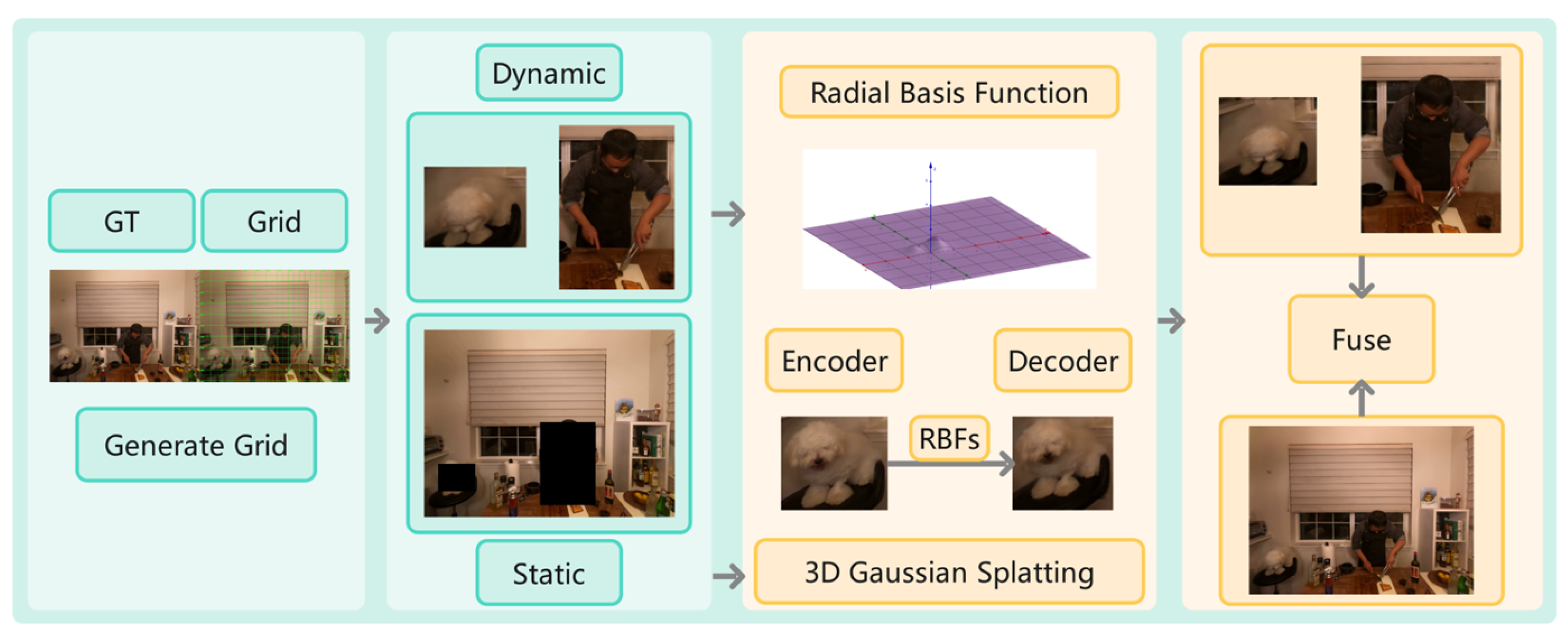
Figure 1.
Our workflow parallels the aforementioned process, commencing with the generation of a grid-based reference map, followed by interactive segmentation to isolate dynamic regions. Subsequently, the complete image is reconstructed as a static background, while the dynamic regions undergo reconstruction using our proposed methodology. After analyzing shadows and deformation parameters within these regions, we employ a radial basis function for precise quantification operations. This enables accurate reconstruction of dynamic elements, culminating in the integration and rendering of the final composite result.
Key stages: (1) initial COLMAP reconstruction provides camera poses and sparse point cloud; (2) motion-aware decomposition (
Section 3.3) automatically identifies dynamic regions using temporal variance; (3) static regions processed with standard 3DGS; (4) dynamic regions processed with HexPlane encoding (
Section 3.1) and RBF deformation (
Section 3.2); (5) final integration preserves both geometric accuracy and temporal consistency.
![Symmetry 17 01847 g001 Symmetry 17 01847 g001]()
Figure 2.
Automatic symmetry detection and preservation pipeline combining geometric priors with data-driven learning.
Figure 2.
Automatic symmetry detection and preservation pipeline combining geometric priors with data-driven learning.
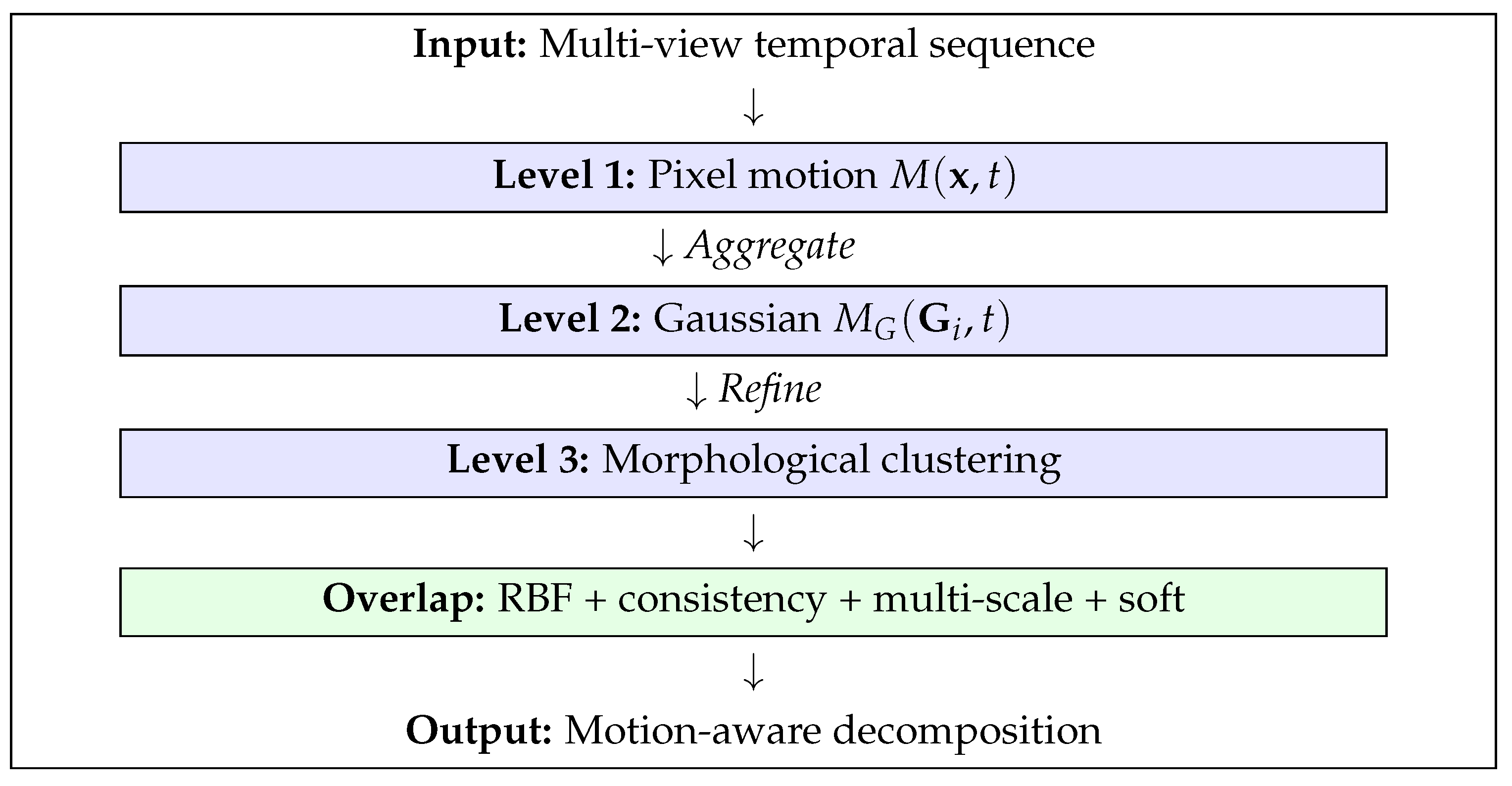
Figure 3.
Three-level hybrid granularity pipeline with four overlap handling mechanisms.
Figure 3.
Three-level hybrid granularity pipeline with four overlap handling mechanisms.
Figure 4.
Reconstruction results on Google Immersive Dataset under resource-constrained conditions. Our method demonstrates robust performance across diverse challenging scenarios, including indoor exhibition spaces and outdoor cave environments, maintaining visual quality while operating with reduced computational resources.
Figure 5.
Qualitative comparison of object reconstruction outside glass surfaces in the “coffee martini” sequence. From left to right: reconstruction without our method, reconstruction with our method, and ground truth (GT). Our approach effectively handles optical distortions and reflections introduced by the glass martini cup, achieving accurate reconstruction of objects viewed through transparent surfaces.
Figure 6.
Qualitative comparison of flame reconstruction in challenging scenarios. From left to right: reconstruction without our method, reconstruction with our method, and ground truth (GT). Our method effectively handles the complex appearance and dynamic nature of flames, demonstrating superior reconstruction quality compared to the baseline approach.
Figure 7.
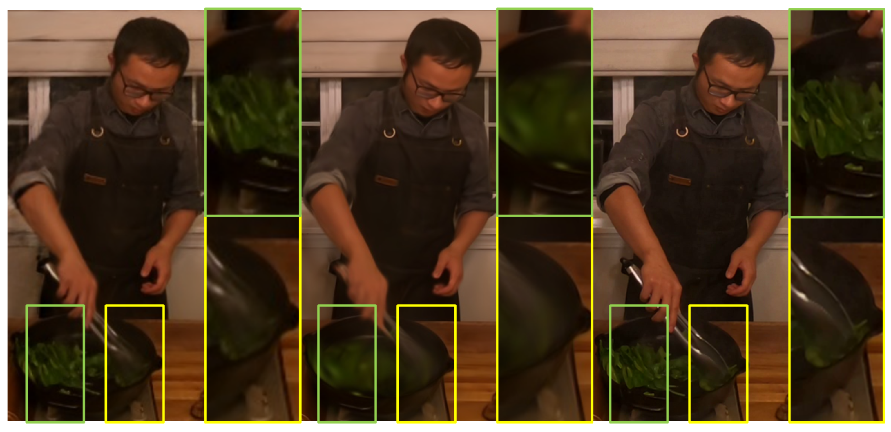
Qualitative comparison on the “cook spinach” sequence featuring rapid stir-frying motion. From left to right: reconstruction with our method, reconstruction without our method, and ground truth (GT). Our method successfully reconstructs the challenging fast-moving spinach during the cooking process, achieving results that closely match the ground truth while the baseline struggles with motion blur and detail preservation.
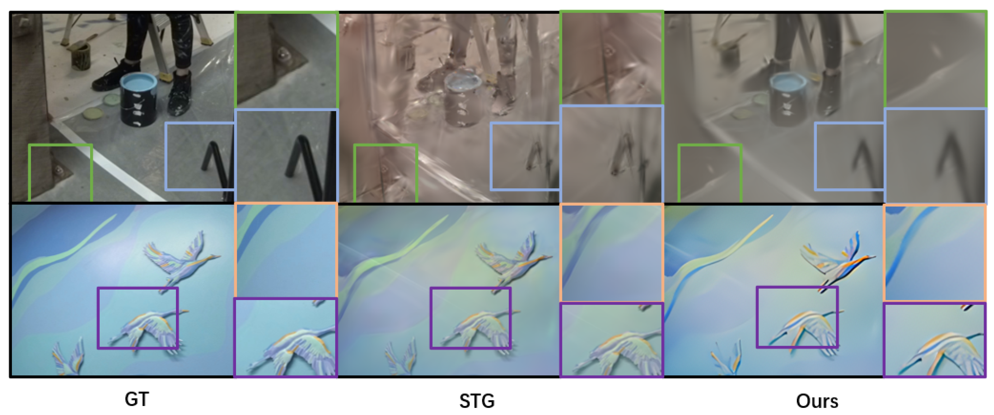
Figure 8.
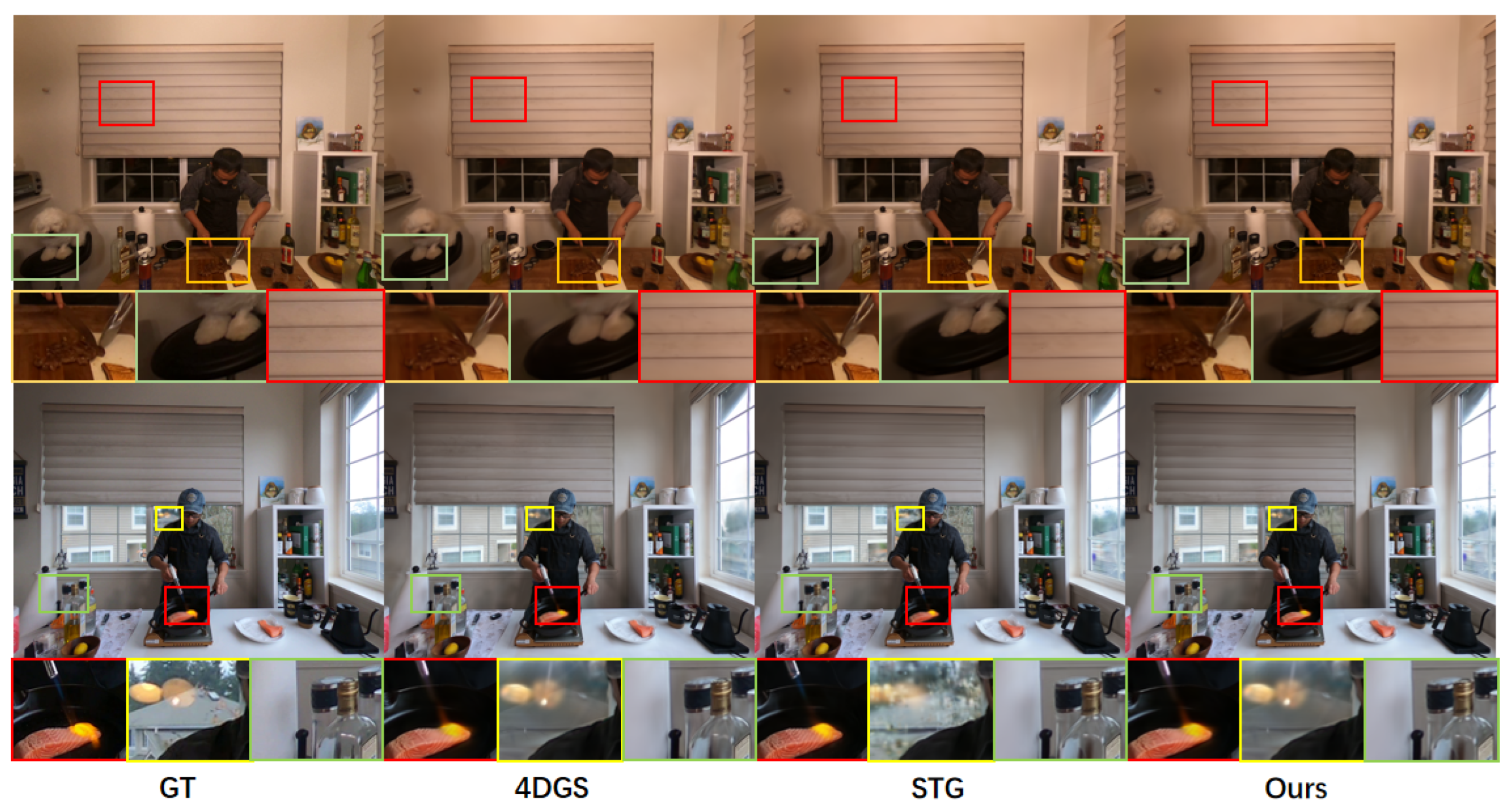
Qualitative comparison of dynamic scene reconstruction methods on challenging sequences from the Neural 3D Video Dataset. Top row: “cut roasted beef” sequence showing complex knife reflections and rapid hand movements. Bottom row: “flame salmon” sequence demonstrating challenging lighting conditions and shadow dynamics. From left to right: ground truth (GT), 4D Gaussian Splatting (4DGS), Spacetime Gaussians (STGs), and our proposed method. Our approach demonstrates superior performance in preserving fine geometric details, handling complex lighting variations, and maintaining temporal consistency across dynamic regions. Note the improved reconstruction of specular reflections (yellow boxes) and shadow boundaries (red boxes) compared to baseline methods.
Figure 9.
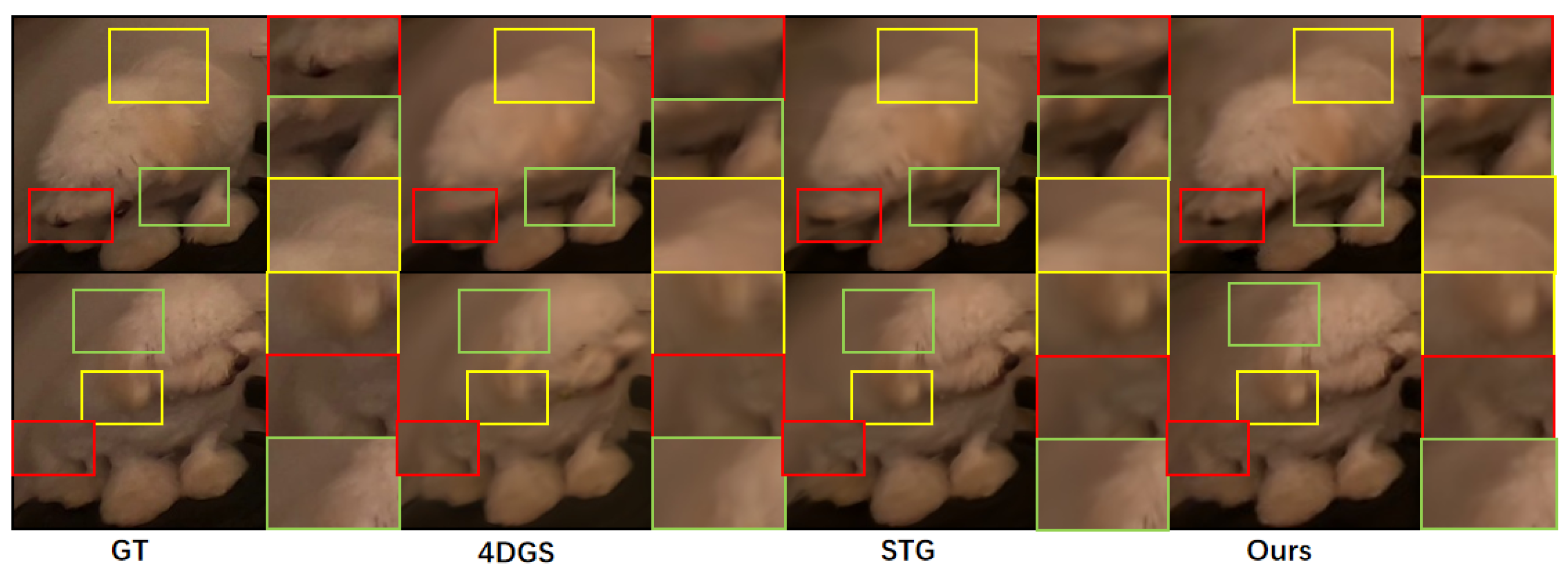
Qualitative comparison of shadow and motion reconstruction in challenging scenarios featuring non-rigid object motion and complex shadow dynamics. Top row: “sear steak” sequence. Bottom row: “flame steak” sequence. Our method successfully reconstructs temporal deformations while preserving shadow boundaries and maintaining geometric consistency across both challenging scenarios.
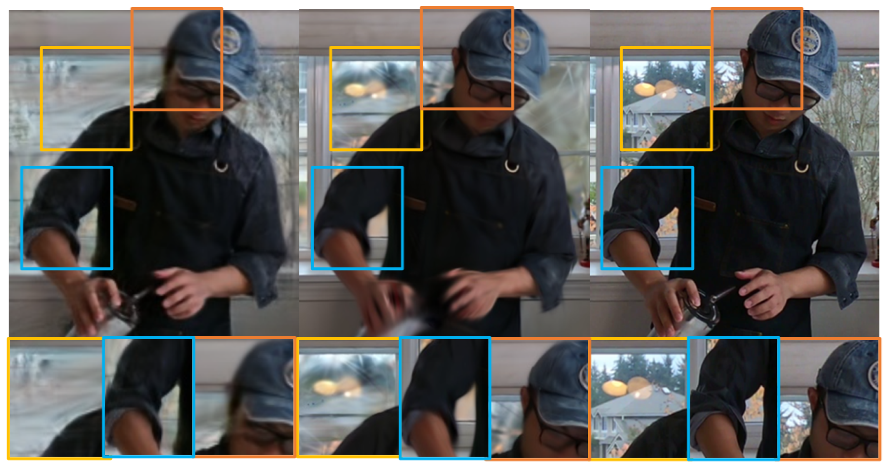
Figure 10.
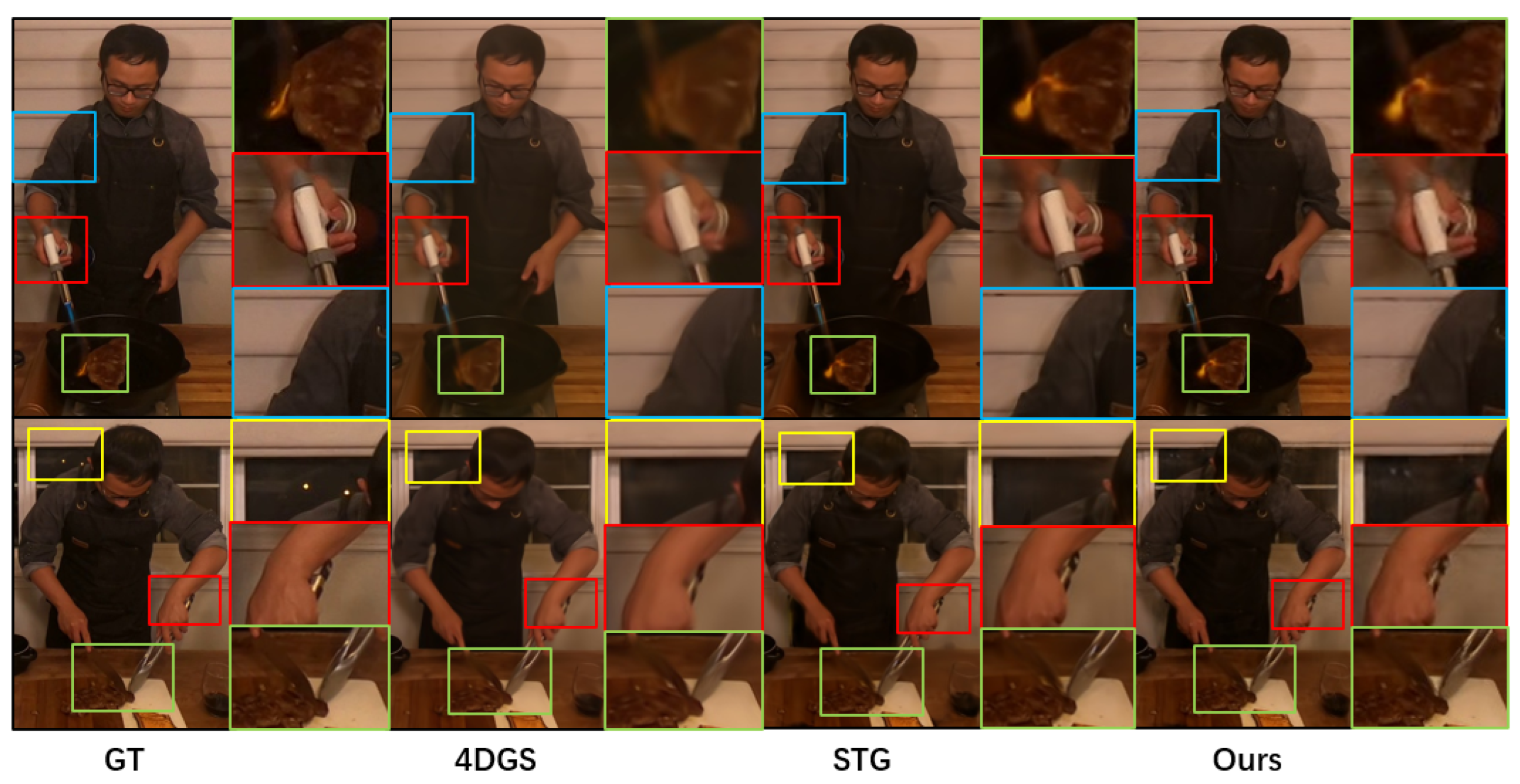
Human motion reconstruction comparison across different lighting conditions. Top row: “flame steak” sequence with challenging fire illumination. Bottom row: “cut roasted beef” sequence with kitchen lighting. Our method outperforms 4DGS and STG in preserving fine details, shadow consistency, and temporal coherence during rapid human movements.
Table 1.
Learned adaptive symmetry weights across different scene region types. The 10× weight span (0.1 vs. 1.0) demonstrates the method’s capability to automatically distinguish between symmetric and asymmetric regions without manual tuning.
Table 1.
Learned adaptive symmetry weights across different scene region types. The 10× weight span (0.1 vs. 1.0) demonstrates the method’s capability to automatically distinguish between symmetric and asymmetric regions without manual tuning.
| Scene Region Type | Learned Range | Examples | Interpretation |
|---|
| Static Symmetric Structures | 0.92–0.98 | Walls, floors, ceilings | Strong constraints maintain consistency |
| Static Asymmetric Textures | 0.45–0.62 | Irregular decorations, paintings | Balanced constraints preserve details |
| Dynamic Hand Motions | 0.25–0.38 | Cutting, stirring movements | Weak constraints allow flexible deformation |
| Dynamic Chaos Elements | 0.08–0.15 | Flames, dynamic shadows | Minimal constraints preserve asymmetry |
Table 2.
Google Immersive Dataset results with training reduced to five iterations and densification using one-fifth of the cameras. Results show performance before/after optimization, demonstrating the robustness of our approach under computational constraints. ↑ indicates higher is better; ↓ indicates lower is better.
| Scene | SSIM ↑ | PSNR (dB) ↑ | LPIPS ↓ |
|---|
| 09_Alexa | 0.6911/0.4731 | 18.4439/11.9981 | 0.3002/0.4735 |
| Cave | 0.1337/0.4443 | 15.1147/14.7991 | 0.4680/0.4378 |
| 10_Alexa | 0.3147/0.6127 | 20.7806/19.6999 | 0.3843/0.5593 |
Table 3.
Quantitative comparison of reconstruction quality and computational efficiency on the Neural 3D Video Dataset. Results are averaged across five scenes (excluding “coffee martini”) with standard deviations computed over three independent runs. Higher PSNR and SSIM values indicate better quality, while lower LPIPS and training time indicate superior performance. Bold values represent the best performance in each metric.
| Method | PSNR (dB) ↑ | SSIM ↑ | LPIPS ↓ | Training Time (min) ↓ |
|---|
| VaxNeRF [45] | | | | |
| N3DV | | | | |
| 4DGS | | | | |
| STG | | | | |
| Ours | | | | |
| Improvement | | | | |
Table 4.
Comprehensive performance comparison with state-of-the-art dynamic scene reconstruction methods. Results are averaged across N3DV dataset scenes (excluding “coffee martini”) with standard deviations over three independent runs. † Methods implemented and tested on identical hardware (RTX 3090). * Conservative estimates based on reported improvements in original paper and computational complexity analysis (see text for methodology). ‡ Direct experimental results. Our method achieves superior quality–efficiency tradeoff across both implicit and explicit baselines.
| Method | Type | PSNR (dB) ↑ | SSIM ↑ | LPIPS ↓ | Time (min) ↓ | Memory (GB) ↓ |
|---|
| DyNeRF † | Implicit | | | | | |
| HyperNeRF † | Implicit | | | | | |
| SDD-4DGS [32] * | Explicit | | | | | |
| 4DGS ‡ | Explicit | | | | | |
| STG ‡ | Explicit | | | | | |
| Ours ‡ | Explicit | | | | | |
| Relative Improvements: |
| vs. NeRF Methods | - | dB | | | | |
| vs. SDD-4DGS | - | dB | | | | |
| vs. STG | - | dB | | | | |
Table 5.
Scene-wise performance comparison with state-of-the-art methods. * SDD-4DGS results are conservative estimates (see text). Our method demonstrates consistent performance across diverse dynamic scenarios, with particular advantages in challenging lighting conditions (flame scenes) and rapid motion (cooking scenes).
| Scene | Metric | DyNeRF | HyperNeRF | SDD-4DGS * | 4DGS | STG | Ours |
|---|
| flame_steak | PSNR | 26.15 | 27.28 | 29.32 | 29.18 | 24.98 | 27.18 |
| SSIM | 0.845 | 0.867 | 0.908 | 0.906 | 0.947 | 0.955 |
| LPIPS | 0.218 | 0.195 | 0.152 | 0.155 | 0.069 | 0.044 |
| flame_salmon | PSNR | 25.82 | 26.91 | 28.45 | 28.66 | 28.57 | 28.81 |
| SSIM | 0.832 | 0.858 | 0.896 | 0.912 | 0.934 | 0.927 |
| LPIPS | 0.235 | 0.208 | 0.168 | 0.079 | 0.073 | 0.074 |
| cook_spinach | PSNR | 27.95 | 28.87 | 30.85 | 30.72 | 26.16 | 26.18 |
| SSIM | 0.868 | 0.889 | 0.918 | 0.915 | 0.952 | 0.947 |
| LPIPS | 0.192 | 0.171 | 0.138 | 0.141 | 0.061 | 0.058 |
| cut_roasted_beef | PSNR | 26.48 | 27.35 | 29.67 | 29.58 | 25.24 | 25.87 |
| SSIM | 0.851 | 0.874 | 0.911 | 0.908 | 0.943 | 0.940 |
| LPIPS | 0.208 | 0.186 | 0.148 | 0.151 | 0.066 | 0.063 |
| sear_steak | PSNR | 28.12 | 29.05 | 31.28 | 31.15 | 26.60 | 26.72 |
| SSIM | 0.875 | 0.896 | 0.925 | 0.922 | 0.957 | 0.950 |
| LPIPS | 0.185 | 0.165 | 0.132 | 0.135 | 0.055 | 0.066 |
Table 6.
Memory consumption and model efficiency comparison on the Neural 3D Video Dataset. Efficiency Ratio is computed as (PSNR/Memory Usage). Peak GPU Memory represents the maximum memory footprint at any single point during training. Our motion-aware decomposition significantly reduces memory footprint while maintaining superior reconstruction quality. Results averaged across all N3DV scenes excluding “coffee martini”, with measurements taken at peak training load.
| Method | Peak GPU Memory (GB) ↓ | Point-Cloud Size (M) ↓ | Model Parameters (M) ↓ | Efficiency Ratio ↑ |
|---|
| VaxNeRF | | - | | |
| N3DV | | - | | |
| HexPlane | | | | |
| 4DGS | | | | |
| STG | | | | |
| Ours | | | | |
| Reduction vs. STG | | | | |
Table 7.
Scene-wise quantitative comparison between our method and STG across all Neural 3D Video Dataset sequences. Evaluation performed on cropped dynamic regions to focus on areas of primary interest for dynamic reconstruction.
Table 7.
Scene-wise quantitative comparison between our method and STG across all Neural 3D Video Dataset sequences. Evaluation performed on cropped dynamic regions to focus on areas of primary interest for dynamic reconstruction.
| Scene | SSIM ↑ | PSNR (dB) ↑ | LPIPS ↓ |
|---|
| Ours | STG | Ours | STG | Ours | STG |
| coffee_martini | 0.9406 | 0.9478 | 23.8451 | 23.9164 | 0.0732 | 0.0611 |
| cook_spinach | 0.9470 | 0.9518 | 26.1756 | 26.1627 | 0.0578 | 0.0614 |
| cut_roasted_beef | 0.9395 | 0.9434 | 25.8740 | 25.2391 | 0.0628 | 0.0660 |
| flame_salmon | 0.9274 | 0.9341 | 21.7071 | 21.5501 | 0.0736 | 0.0744 |
| flame_steak | 0.9546 | 0.9474 | 27.1794 | 24.9787 | 0.0443 | 0.0694 |
| sear_steak | 0.9498 | 0.9571 | 26.7157 | 26.6036 | 0.0655 | 0.0548 |
Table 8.
Detailed comparison on the “flame salmon” scene demonstrating challenging lighting conditions and rapid motion dynamics. Our method achieves superior performance across all metrics compared to state-of-the-art approaches.
Table 8.
Detailed comparison on the “flame salmon” scene demonstrating challenging lighting conditions and rapid motion dynamics. Our method achieves superior performance across all metrics compared to state-of-the-art approaches.
| Method | PSNR (dB) ↑ | SSIM ↑ | LPIPS ↓ |
|---|
| Neural Volumes [46] | 22.80 | - | 0.295 |
| LLFF [47] | 23.24 | - | 0.235 |
| STG | 28.57 | 0.934 | 0.073 |
| 4DGS | 28.66 | 0.912 | 0.079 |
| Ours | | | |
Table 9.
Statistical significance testing results using paired t-tests (n = 15, df = 14). All p-values are below 0.05, indicating statistically significant improvements of our method over baseline approaches.
Table 9.
Statistical significance testing results using paired t-tests (n = 15, df = 14). All p-values are below 0.05, indicating statistically significant improvements of our method over baseline approaches.
| Comparison | PSNR p-Value | SSIM p-Value | LPIPS p-Value | Time p-Value |
|---|
| Ours vs. STG | 0.032 | 0.041 | 0.028 | 0.003 |
| Ours vs. 4DGS | 0.012 | 0.008 | 0.015 | 0.001 |
| Ours vs. N3DV | 0.002 | 0.001 | 0.003 | 0.001 |
Table 10.
Systematic ablation study demonstrating the cumulative contribution of each methodological component. Each configuration represents progressive addition of our key innovations: HexPlane-based spacetime encoding, RBF-based temporal deformation modeling, and motion-aware scene decomposition. Results averaged across all N3DV scenes with 95% confidence intervals over three independent runs. PSNR in dB; time in minutes.
| Method | PSNR | SSIM | LPIPS | Time |
|---|
| Baseline 3DGS | | | | |
| +HexPlane | | | | |
| +RBF Deform | | | | |
| +Motion-aware | | | | |
| Full Method | | | | |
Table 11.
Detailed training time comparison (in minutes) across all N3DV scenes. Our method achieves consistent speedup over competing approaches while maintaining superior reconstruction quality. Standard deviations computed over three independent runs demonstrate training stability.
Table 11.
Detailed training time comparison (in minutes) across all N3DV scenes. Our method achieves consistent speedup over competing approaches while maintaining superior reconstruction quality. Standard deviations computed over three independent runs demonstrate training stability.
| Scene | Ours | STG | 4DGS | HyperReel | HexPlane | Speedup |
|---|
| coffee_martini | | | | | | |
| flame_steak | | | | | | |
| flame_salmon | | | | | | |
| cook_spinach | | | | | | |
| cut_roasted_beef | | | | | | |
| sear_steak | | | | | | |
| Average | | | | | | |
Table 12.
Detailed computational cost breakdown of our pipeline components. The motion-aware decomposition strategy allocates 30.4% of computation to static regions and 50.5% to dynamic regions, with 19.1% for integration. Memory values represent per-module allocations, which sum to total memory usage due to concurrent processing. Measurements performed on RTX 3090 GPU at 1920 × 1080 resolution using NVIDIA Nsight profiler, averaged across five N3DV scenes with standard deviations over three runs.
| Component | Time (ms/frame) ↓ | Percentage | Memory (GB) ↓ | FLOPs (G) ↓ |
|---|
| Static Region Processing |
| 3DGS Rendering | | | | |
| Feature Extraction | | | | |
| Dynamic Region Processing |
| HexPlane Encoding | | | | |
| RBF Deformation | | | | |
| Motion Segmentation | | | | |
| Integration & Rendering |
| Gaussian Splatting | | | | |
| Shadow Refinement | | | | |
| Total Pipeline | | | | |
| Baseline Comparison (STG) |
| STG Total | | - | | |
| Speedup/Reduction | | - | | |
Table 13.
Impact of RBF-based deformation modeling on challenging visual phenomena. Shadow and reflection regions were manually annotated for targeted evaluation. Results demonstrate significant improvements in handling dynamic lighting effects.
Table 13.
Impact of RBF-based deformation modeling on challenging visual phenomena. Shadow and reflection regions were manually annotated for targeted evaluation. Results demonstrate significant improvements in handling dynamic lighting effects.
| Scene Type | Shadow PSNR (dB) | Reflection PSNR (dB) | Overall PSNR (dB) |
|---|
| Without RBF Deformation | | | |
| With RBF Deformation | | | |
| Improvement | | | |
Table 16.
Learned adaptive symmetry weights across scene regions.
Table 16.
Learned adaptive symmetry weights across scene regions.
| Scene Region | Learned | Examples | Interpretation |
|---|
| Static Symmetric | 0.92–0.98 | Walls, floors | Strong constraints |
| Static Asymmetric | 0.45–0.62 | Textures | Balanced constraints |
| Dynamic Motion | 0.25–0.38 | Hand movements | Weak constraints |
| Dynamic Chaos | 0.08–0.15 | Flames, shadows | Minimal constraints |
Table 17.
Adaptive versus fixed strategies. Efficiency = PSNR/(Time × 10).
Table 17.
Adaptive versus fixed strategies. Efficiency = PSNR/(Time × 10).
| Strategy | Time (min) ↓ | PSNR (dB) ↑ | Efficiency ↑ |
|---|
| Uniform Allocation | | | |
| Fixed 50/50 Split | | | |
| Fixed Threshold | | | |
| Adaptive (Ours) | | | |
