Abstract
This study applies reinforcement learning to search parameter regimes that yield chaotic dynamics across six systems: the Logistic map, the Hénon map, the Lorenz system, Chua’s circuit, the Lorenz–Haken model, and a custom 5D hyperchaotic design. The largest Lyapunov exponent (LLE) is used as a scalar reward to guide exploration toward regions with high sensitivity to initial conditions. Under matched evaluation budgets, the approach reduces redundant simulations relative to grid scans and accelerates discovery of parameter sets with large positive LLE. Experiments report learning curves, parameter heatmaps, and representative phase portraits that are consistent with Lyapunov-based assessments. Q-learning typically reaches high-reward regions earlier, whereas SARSA shows smoother improvements over iterations. Several evaluated systems possess equation-level symmetry—most notably sign-reversal invariance in the Lorenz system and Chua’s circuit models and a coordinate-wise sign pattern in the Lorenz–Haken equations—which manifests as mirror attractors and paired high-reward regions; one representative is reported for each symmetric pair. Overall, Lyapunov-guided reinforcement learning serves as a practical complement to grid and random search for chaos identification in both discrete maps and continuous flows, and transfers with minimal changes to higher-dimensional settings. The framework provides an efficient method for identifying high-complexity parameters for applications in chaos-based cryptography and for assessing stability boundaries in engineering design.
1. Introduction
Chaotic systems exhibit strong sensitivity to initial conditions and parameter variations, resulting in highly complex and unpredictable dynamical behavior. Owing to their inherent nonlinearity and structural richness, such systems have been extensively investigated in physics, engineering [1], and cryptography [2]. The nonlinear and high-dimensional nature of these systems further complicates comprehensive exploration using classical analytical approaches.
The identification of parameter regimes that induce chaos is not merely an academic exercise; it is a critical component for several practical applications. In chaos-based cryptography, the security and robustness of encryption algorithms, particularly for tasks like image encryption [3], depend directly on the complexity and unpredictability of the underlying chaotic system [4]. Discovering parameters that generating high-quality pseudo-random sequences and ensuring resilience against attacks [5]. Similarly, in physics and engineering, the ability to efficiently map chaotic regions is vital for both system design and complexity analysis. This capability is necessary for tasks such as inducing chaos to enhance mixing in fluid dynamics [6], or conversely, avoiding chaotic regimes to ensure the stability of mechanical structures or electrical systems. The primary challenge in these applied tasks is to meet realistic performance demands. This often requires locating sparse, narrow, or intricately structured chaotic regions within vast, high-dimensional parameter spaces [7]. For such tasks, traditional discovery methods, such as comprehensive grid-based parameter sweeps or plotting multi-parameter bifurcation diagrams, suffer from the curse of dimensionality. These brute-force approaches scale poorly, quickly becoming computationally prohibitive and inefficient as the number of system parameters increases, rendering the exhaustive exploration of the complete parameter space infeasible [8].
Several of the studied models exhibit equation-level symmetry that organizes both the attractor geometry and the reward landscape. In the Lorenz equations, sign-reversal invariance produces mirror attractors with identical Lyapunov estimates. Chua’s circuit, with an odd piecewise-linear nonlinearity, shows the same property around the origin. The Lorenz–Haken model preserves a coordinate-wise sign pattern, leading to paired structures in phase-space projections.
To address these limitations, reinforcement learning (RL) has emerged as a promising alternative for navigating parameter spaces in dynamical systems [9]. By formulating the search for chaotic regimes as a sequential decision-making task, reinforcement learning agents can adaptively select parameter combinations that maximize a formal measure of chaos. The largest Lyapunov exponent (LLE), a widely accepted indicator of chaotic divergence, is utilized as a continuous scalar reward signal [10]. Compared to brute-force methods, reinforcement learning offers adaptive sampling and enhanced convergence toward chaos-inducing parameter sets, thereby improving both efficiency and scalability [11].
This comparison reveals a clear research gap: while reinforcement learning has been successfully applied to control chaotic systems, its use as an efficient, autonomous discovery tool for mapping vast, high-dimensional parameter spaces remains underexplored. This gap motivates the following research question (RQ): Can an RL agent that uses the largest Lyapunov exponent (LLE) as its reward efficiently and autonomously discover sparse chaotic regimes in high-dimensional nonlinear dynamical systems, and does it offer a quantifiable advantage over traditional brute-force methods? An LLE-based RL framework is adopted because it aligns the agent’s learning objective (reward maximization) with a fundamental indicator of chaos, thereby enabling adaptive, sample-efficient exploration of parameter landscapes.
Model-free reinforcement learning algorithms [12], such as Q-learning and SARSA (state–action–reward–state–action) [13], are employed to autonomously discover chaotic behavior in a broad spectrum of classical and hyperchaotic systems. Q-learning, an off-policy method, estimates the optimal action value function independently of the current policy, promoting the fast exploration of high-reward regions [14]. In contrast, SARSA updates estimates based on the agent’s actual behavior, favoring more stable and conservative learning. Comparatively integrating these two strategies allows for a systematic evaluation of the exploration–stability trade-off in chaotic parameter identification. The framework identifies parameter settings that yield chaotic behavior, supported by numerical simulations and attractor plots.
The principal contributions of this study are summarized as follows:
- (i)
- A unified reinforcement learning-based framework for discovering chaotic parameters in multiple nonlinear dynamical systems;
- (ii)
- The integration of Lyapunov exponents as continuous reward signals for training reinforcement learning agents;
- (iii)
- An empirical comparison between Q-learning and SARSA in terms of convergence, reward profiles, and attractor richness across various systems.
This paper is organized as follows: Section 2 presents the reinforcement learning framework, including the SARSA and Q-learning algorithms. Section 3 describes the proposed methodology and experimental setup. Section 4 provides the results and discussion. Section 5 discusses these results in the context of prior work and practical applications. Section 6 concludes the paper and suggests future research directions.
2. Reinforcement Learning for Chaotic Parameter Exploration
This section presents the RL framework designed to identify chaos-inducing parameter regions in nonlinear dynamical systems. System parameters are encoded within the state–action space, and the LLE is employed as a scalar reward signal [15]. Two representative RL algorithms, Q-learning and SARSA, are introduced, followed by the formulation of the reward function. A comparison with traditional numerical techniques highlights the advantages of the proposed learning-based strategy.
2.1. Formal Problem Definition
The parameter search as a discrete-time Markov Decision Process (MDP). The agent’s goal is to find an optimal policy that maximizes the expected discounted sum of future rewards (the return), , defined as
where is the reward at time t, and is the discount factor.
The action-value function is the expected return for taking action a in state s and thereafter following policy . The optimal action-value function must satisfy the Bellman optimality equation [16]:
This equation forms the theoretical basis for the Q-learning algorithm. As the problem is defined by discrete, episodic parameter evaluations (one LLE calculation per action), this discrete-time Bellman equation is the appropriate foundation, rather than the continuous-time Hamilton–Jacobi–Bellman (HJB) equation [17].
2.2. Previous RL Applications in Chaotic Systems
An adaptive RL approach has been proposed for chaotic systems governed by nonlinear differential equations [18]. The method assumed bounded but unknown nonlinearities, with the bounds estimated online. Neural networks were used to approximate the reinforcement signal, and control synthesis was achieved through Lyapunov stability theory and Young’s inequality. The primary objective was controller stabilization rather than an exploratory parameter search.
Reinforcement learning has also been applied to chaos control. For example, Q-learning has been employed to construct both control and anti-control strategies for systems such as the Lorenz attractor and Hénon map [19]. The LLE served as a reward to tune system parameters and modulate chaoticity [20]. Although this study demonstrated reinforcement learning viability in chaotic environments, the focus remained on regulating system trajectories.
More recently, research has explored reinforcement learning in partially observable chaotic systems, applying the framework to the Kuramoto–Sivashinsky equation [21]. Recurrent and transformer-based policy networks were compared for memory encoding, with attention mechanisms outperforming in highly chaotic regimes.
Beyond control and stabilization, recent work has explored RL for parameter estimation and adaptive prediction in chaotic environments. For instance, some studies combine machine learning techniques with synchronization methods to estimate unknown parameters from chaotic time series data [22], a crucial step for subsequent control or analysis. Other research leverages RL for adaptive time-stepping in chaotic simulations, where the agent learns to dynamically adjust integration parameters to balance accuracy and computational cost [23].
In contrast, the present study focuses on autonomous parameter space exploration for chaos discovery rather than stabilization or control [24]. The LLE is used as a direct reward measure of chaotic behavior under full state observability [25].
These distinctions establish the proposed framework as a general-purpose methodology for chaos identification, with applications in system discovery, complexity analysis, and secure system design [26].
2.3. SARSA Algorithm
SARSA is an on-policy temporal difference method that updates the action value function based on actions executed under the current policy [27]. At each time step, the agent transitions from state to by executing action and selects the subsequent action using the same policy [28].
The update rule is defined as
where denotes the learning rate and is the discount factor. Policy-consistent updates contribute to stable convergence, making SARSA suitable in scenarios where real-time policy adherence is desirable [29]. The convergence of tabular SARSA to the optimal policy is guaranteed as long as all state-action pairs continue to be visited, a condition satisfied by an -greedy policy [30].
SARSA is included in this study primarily as an on-policy baseline. We evaluate it to determine if its more conservative, policy-dependent updates offer greater stability when navigating the potentially sharp and narrow reward landscapes found in chaotic parameter spaces.
2.4. Q-Learning Algorithm
Q-learning is an off-policy temporal difference method that estimates the optimal action value function independently of the policy used during training [31]. The update rule is as follows [32]:
This greedy update mechanism promotes faster convergence to high-reward regions, particularly in sparse or high-dimensional spaces [33]. Tabular Q-learning is proven to converge to the optimal action-value function with probability 1, provided all state-action pairs are visited infinitely and a proper learning rate schedule is used [34].
Q-learning is the primary algorithm of interest for this discovery task. Its off-policy nature is a significant advantage, as it allows the agent to learn the optimal value function independently of the exploration policy. This is ideal for a parameter search, where we desire efficient, and at times aggressive, exploration (e.g., -greedy) without corrupting the learned value of the optimal “chaos-inducing” policy.
2.5. Reward Function Design
The reward function provides the primary learning signal for reinforcement learning agents [35]. In this study, the LLE is used to quantify the degree of chaos, serving as a scalar reward. Positive values of reflect the exponential divergence of nearby trajectories [36], which is a fundamental property of chaotic systems.
To enhance reward signal resolution and ensure numerical stability, the exponentiated form of the Lyapunov exponent is used in higher-dimensional systems:
where denotes the selected parameter set. This transformation ensures all rewards remain positive and amplifies small differences in near the chaotic threshold, facilitating more efficient exploration in large parameter spaces.
Using the LLE as the reward signal is the core methodological choice that connects the RL agent’s objective to the physical definition of chaos. The transformation in Equation (5) is a critical design feature to handle reward sparsity, ensuring that the agent can differentiate between weakly chaotic (small ) and strongly chaotic (large ) regimes, rather than treating all chaos as a simple binary reward.
For lower-dimensional systems, where chaotic regimes are well-defined and more easily separable, the untransformed Lyapunov exponent is sufficient:
This adaptive reward function promotes the discovery of parameter configurations that exhibit sustained chaos while implicitly penalizing periodic or fixed-point dynamics. Regularization terms such as could be introduced near the edge of chaos to avoid vanishing gradients and improve learning stability.
2.6. Advantages over Traditional Numerical Analysis
Conventional approaches to chaotic parameter discovery, such as grid-based parameter sweeps, bifurcation diagrams, and Lyapunov surface visualizations, often require expert intervention and extensive computational cost.
In contrast, the reinforcement learning-based framework provides several key advantages, which are experimentally quantified in Section 4.1. The primary advantages are as follows:
- An adaptive exploration of parameter regions with higher chaotic potential based on experience.
- The reuse of evaluated configurations to inform future decisions and reduce redundancy.
- Scalability to high-dimensional systems.
- Autonomous operation without reliance on heuristic or manual tuning strategies.
By combining Lyapunov-guided rewards with sample-efficient policy updates, the framework enables self-directed learning in complex dynamical environments, offering a scalable and generalizable solution for chaos identification. A summary contrasting the algorithms regarding their relevance to parameter discovery is provided in Table 1.

Table 1.
Condensed comparison of methods for chaotic parameter discovery under matched evaluation budgets.
3. Methodology
This section outlines the chaotic systems investigated, the Lyapunov-based reward function, and the implementation details of the reinforcement learning process. A unified framework is applied to all systems to ensure consistency and scalability.
3.1. Chaotic System Models
The six following dynamical systems are included, chosen to represent a range of dimension and behaviors from classic 1D maps to hyperchaotic system flows:
- Logistic Map (1D) [37]: A discrete-time model that serves as a canonical example of how complex, chaotic behavior can arise from a simple nonlinear iterative equation. It is defined bywhere and r is the bifurcation parameter.
- Hénon Map (2D) [38]: A classic 2D discrete-time dynamical system that is well-known for exhibiting a strange attractor. Its equation is given bywith control parameters a and b.
- Lorenz System (3D) [39]: A simplified mathematical model for atmospheric convection, notable for its “butterfly” strange attractor, which was one of the first systems to demonstrate deterministic chaos. It is defined bywhere , , and are adjustable parameters.
- Chua’s Circuit (3D) [40]: A simple electronic circuit that exhibits a wide range of nonlinear dynamics, including bifurcations and chaos, making it a standard benchmark. Its dynamics are governed bywith a piecewise linear function modeling the nonlinear resistor.
- Lorenz–Haken System (4D) [41]: A model that describes the dynamics of a single-mode laser, often used to study instabilities and chaos in optical systems. Its equations are given bywhere , , r, and b are system parameters.
- Custom 5D Hyperchaotic System: A high-dimensional system designed for this study to test scalability and performance in a hyperchaotic regime. It is defined bywhich is constructed by embedding a Lorenz-like core into a 5D structure with nonlinear interactions and auxiliary feedback states. This model yields multiple positive Lyapunov exponents and high-dimensional attractors.
3.2. Numerical Integration
All continuous systems are integrated using the fourth-order Runge–Kutta (RK4) method with a fixed time step of [42]. The RK4 algorithm is defined as
This method was chosen because RK4 offers a standard balance between accuracy and predictable computational cost for simulating chaotic systems [43]. Its higher order accuracy (global error vs. Euler’s ) is crucial for chaos, where errors amplify quickly. Furthermore, the fixed step size ensures a consistent cost per LLE evaluation, which is better suited for the tabular RL framework than adaptive step-size methods.
3.3. Search Space and Training Settings
Parameter ranges for each chaotic system are discretized, as shown in Table 2. Each episode selects a parameter vector from the discrete set, runs a short simulation, and estimates the LLE as the scalar reward. Q-values over the discrete candidates are updated using either SARSA or Q-learning under -greedy behavior. Protocol details and hyperparameters are summarized in Table 3.
Table 2.
Parameter space discretization used in the experiments.
Table 3.
Training protocol and hyperparameters.
All experiments reported in this study were conducted as software simulations. The computing hardware used was an Intel Core i9-13900K processor with 64 GB of RAM, running Windows 11 Pro. The primary focus of the analysis remains on the sample efficiency (number of evaluations) rather than specific execution times or detailed resource utilization, as these can vary significantly based on implementation details.
4. Experimental Results and Analysis
This section reports an evaluation of the proposed reinforcement learning framework on a collection of six chaotic systems. The analysis covers learning performance, attractor reconstruction, and algorithm comparison. The results are organized into subsections detailing the evaluated systems, the observed training performance, and the final attractor reconstructions.
4.1. Quantitative Baseline Comparison
A primary claim of this study is that RL-based exploration reduces redundant simulations compared to a brute-force grid scan. To quantitatively verify this, define computational cost as the number of LLE evaluations required. For a grid search, this is the total number of points in the discretized space (from Table 1). For the RL agents, this is the number of episodes (evaluations) required to consistently find parameter regions with a high positive LLE (estimated from Figure 1, Figure 2, Figure 3, Figure 4, Figure 5 and Figure 6).
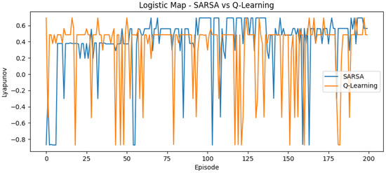
Figure 1.
Reward curve for logistic map using SARSA and Q-learning.
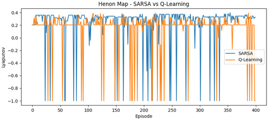
Figure 2.
Reward curve for Hénon map using SARSA and Q-learning.
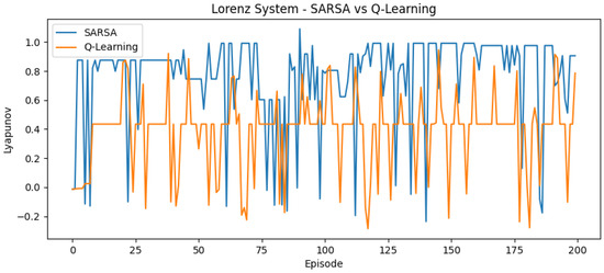
Figure 3.
Reward curve for Lorenz system using SARSA and Q-learning.
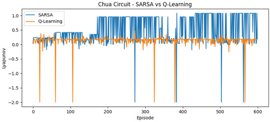
Figure 4.
Reward curve for Chua circuit using SARSA and Q-learning.
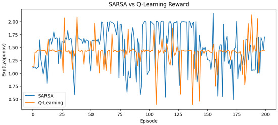
Figure 5.
Reward curve for Lorenz–Haken system using SARSA and Q-learning.
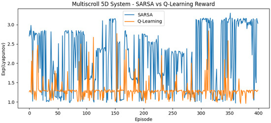
Figure 6.
Reward curve for 5D hyperchaotic system using SARSA and Q-learning.
Table 4 provides a direct experimental comparison. As shown in the table, the 1D Logistic map, with only 100 candidate points, serves as a low-dimensional benchmark where the search space is too small to offer a significant advantage for RL over a grid scan; the experimental run (200 episodes) simply explored this small space thoroughly, resulting in no cost reduction.
Table 4.
Comparison of computational cost (number of LLE evaluations).
However, for all systems 2D and higher, the efficiency gain is substantial. For instance, in the 5D hyperchaotic system, the agents found high-LLE parameters within approximately 100–150 episodes, a >98% reduction in cost compared to the 10,000-point baseline. This demonstrates that the agent’s adaptive exploration policy effectively avoids redundant evaluations of non-chaotic regions and scales efficiently to high-dimensional systems.
4.2. Overview of Evaluated Systems
The experimental systems span a wide spectrum of nonlinear behaviors and dimensionalities, providing a broad benchmark for parameter search in chaotic dynamics. The two discrete-time maps—the logistic map and the Hénon map—serve as classical low-dimensional cases defined by iterative equations and are assessed via Jacobian-based LLE estimates.
The continuous-time set includes the Lorenz system, Chua’s circuit, the Lorenz–Haken laser model, and a designed 5D hyperchaotic system. These systems are simulated using the fourth-order Runge–Kutta method, with chaos identified through positive LLE estimates and corroborating attractor reconstructions.
All systems are trained independently under tabular Q-learning and SARSA using a unified pipeline, a common parameter discretization strategy, and the same reward definition. This design supports comparability across models and consistency in algorithm behavior. System-specific settings, including parameter ranges and integration details, are provided in the methodology section.
4.3. Training Performance and Reward Convergence
Figure 1, Figure 2, Figure 3, Figure 4, Figure 5 and Figure 6 show combined reward curves for each system under Q-learning and SARSA. The reward is a monotone transform of the largest Lyapunov exponent (LLE) used to reflect how often the methods reach parameter regions associated with chaotic behavior.
In the logistic and Hénon maps, both methods converge within ≈200 episodes. SARSA exhibits slightly higher variance, while Q-learning stabilizes earlier. Fast convergence is expected in these low-dimensional, discrete-time settings.
For the Lorenz system, Chua’s circuit system, and Lorenz–Haken system, both methods gradually reach regions linked to a positive LLE. SARSA is more responsive to early signals and can overshoot transiently; Q-learning shows steadier increases. In Chua’s circuit, SARSA displays early peaks that are not consistently sustained, while Q-learning tends to remain near boundary regions, consistent with the difficulty posed by narrow chaotic windows.
For the 5D multi-scroll hyperchaotic model, the parameter space is larger and reward fluctuations persist longer. Both methods eventually reach high-reward regions, with SARSA benefiting from on-policy updates and Q-learning improving more slowly under the fixed budget.
4.4. Attractor Reconstruction and Chaotic Behavior
To verify the emergence of chaotic dynamics under the learned parameters, phase space trajectories were visualized for each system. These attractor plots serve as a qualitative confirmation of chaos, complementing the Lyapunov-based reward signal. For discrete-time systems, iteration results are directly plotted. For continuous systems, the final trajectories after integration using the fourth-order Runge–Kutta method are displayed.
In the logistic map (Figure 7), both Q-learning and SARSA produced state sequences that densely occupied the available phase space.
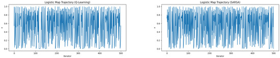
Figure 7.
Attractors generated by learned parameters in the logistic map.
In the Hénon map (Figure 8), attractors resemble the canonical horseshoe structure, demonstrating sensitivity to initial conditions and non-periodicity.
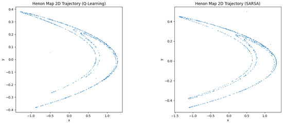
Figure 8.
Attractors generated by learned parameters in the Henon map.
For Chua’s circuit in Figure 9, the reconstructed 3D trajectoriesunder SARSA spiraled toward a fixed point rather than forming a multi-scroll attractor. However, Q-learning successfully located parameters that generate the canonical double-scroll attractor. Although reward signals were obtained during training, the dynamics indicate convergence to parameters near the edge of chaos, likely in periodic or marginally stable regimes. In contrast, the trajectory under SARSA converged the results in a stable fixed point.
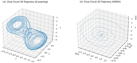
Figure 9.
Attractors generated by learned parameters in the Chua’s circuit system.
The Lorenz system, as shown in Figure 10, yielded the classical double-scroll attractor under both algorithms.
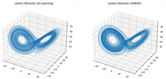
Figure 10.
Attractors generated by learned parameters in the Lorenz system.
Figure 11 and Figure 12 show pairwise projections of trajectories under learned parameters for the Lorenz–Haken system. Q-learning (Figure 11) covers broader regions with visible folding and stretching, whereas SARSA (Figure 12) forms tighter loops with smoother occupancy around the main sheets. These patterns are consistent with positive largest Lyapunov exponent estimates and non-repeating local geometry. Figure 13 presents three-dimensional projections exhibiting layered sheets and lobe-like structures characteristic of chaotic motion in this model.
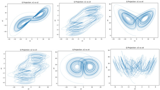
Figure 11.
Attractors generated by learned parameters from Q-learning in the Lorenz–Haken system for 2D projection.
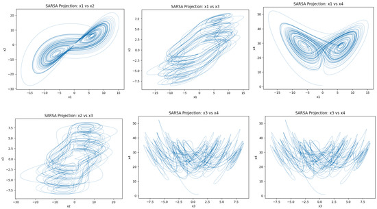
Figure 12.
Attractors generated by learned parameters from SARSA learning in the Lorenz–Haken system for 2D projection.
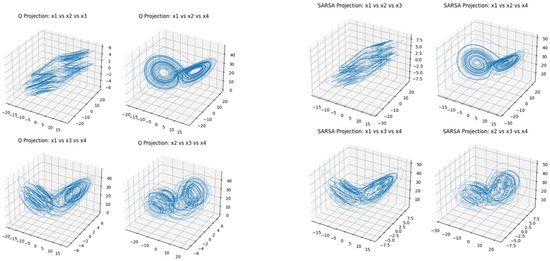
Figure 13.
Attractors generated by learned parameters in the Lorenz–Haken system for 3D projection.
The 5D hyperchaotic system, constructed with sinusoidal nonlinearities, demonstrates intricate chaotic attractors under both SARSA and Q-learning. As shown in Figure 14 and Figure 15, the 2D phase projections reveal continuously folding trajectories with irregular returns, characteristic of chaotic motion. The corresponding 3D attractors in Figure 16 display volumetric expansion and intertwined spirals, indicative of multi-scroll dynamics and inter-variable feedback.
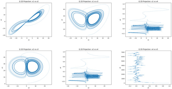
Figure 14.
Attractors generated by learned parameters from Q-learning in the 5D system for 2D projection.
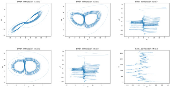
Figure 15.
Attractors generated by learned parameters from SARSA in the 5D system for 2D projection.
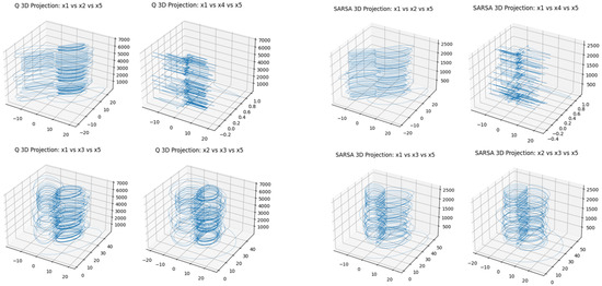
Figure 16.
Attractors generated by learned parameters in the 5D system for 3D projection.
5. Discussion
This section analyzes the experimental findings from Section 4, compares them to related work, and discusses their practical implications and inherent limitations.
5.1. Summary of Experimental Findings
This subsection consolidates the main experimental outcomes observed across the six benchmark systems. Table 5 provides a comparative overview, summarizing the number of episodes required for the RL agents to consistently identify high-LLE regions, the qualitative assessment of the resulting attractor’s structure and the key performance differences noted between the Q-learning and SARSA algorithms.
Table 5.
Consolidated summary of experimental findings.
The approximate training times are provided in Table 6, illustrating the practical duration for each simulation run.
Table 6.
Approximate RL training times.
5.2. Comparison with Related Work and Practical Implications
The framework applies RL to the problem of parameter discovery, which distinguishes it from prior studies that focused on RL for chaos stabilization or trajectory control. Because these studies did not aim to comprehensively map chaotic parameter regimes, a direct comparison of search results is less relevant than comparing the findings to the traditional numerical methods the framework seeks to complement: grid-based parameter sweeps and bifurcation analysis [44].
This study’s results demonstrate a clear efficiency gain over such brute-force methods. A traditional grid scan must evaluate every single candidate point, resulting in massive computational cost that suffers from the curse of dimensionality [45]. This is particularly true for multi-parameter bifurcation analysis, which becomes computationally prohibitive and exceedingly difficult as the number of system parameters increases. For instance, the discretized Lorenz parameter space contained (8000) candidate, while the Lorenz-Haken and 5D systems each had (10,000) candidates. In contrast, the RL agents located high-LLE regions for the Lorenz system within approximately 200 episodes and for the Hénon map within 300 episodes. This represents a small fraction of the total search space, confirming that the Lyapunov-guided RL approach successfully reduces redundant simulations through adaptive exploration. This superior sample efficiency [46] is precisely what enables scalability to the 4D and 5D systems, for which an exhaustive 10,000-point grid scan would be computationally infeasible under the same evaluation. While finding high-LLE regions can be framed as an optimization task potentially addressable by metaheuristics, the contribution of RL lies in learning an adaptive sequential sampling policy from experience, offering a different paradigm compared to many population-based optimizers and demonstrating significant efficiency gains over brute-force methods as shown here.
5.3. Analysis of the Chua’s Circuit Case: Algorithmic Limitations and Landscape Topology
A divergent performance was observed in the Chua’s circuit experiment. The Q-learning agent identified parameters that generated a double-scroll chaotic attractor, as shown in Figure 9a. In contrast, the SARSA agent, operating under the same evaluation budget and parameter grid, converged to parameters that resulted in a stable fixed point as shown in Figure 9b.
This failure of SARSA highlights a limitation of tabular methods for this system’s reward landscape, which is believed to contain narrow chaotic windows. This landscape topology interacts critically with our discretization grid and the specific update rules. Q-learning’s optimistic update rule updates its value based on the maximum expected future reward (). This allows it to identify and propagate the value of a high-reward (chaotic) state, even if the -greedy exploration policy often steps out of that narrow window.
Conversely, SARSA’s policy-dependent update uses the value of the next action chosen by its exploration policy (). When exploring a narrow reward peak, an exploratory for the next action will frequently land in an adjacent low-reward (stable) region, which ’averages down’ the value estimate for the chaotic state. This comparison suggests SARSA’s more conservative update rule struggled to stabilize on the narrow reward peak, converging instead to the broader, suboptimal fixed-point region. Q-learning’s optimistic update proved more effective for this discovery task.
This case identifies a clear limit of the tabular approach, especially when grid resolution is coarse. A neural network for employing deep reinforcement learning approaches, such as Deep Q-Networks (DQN), it could learn a value function over the continuous parameter space. This would remove the dependency on a prior discretization and thus potentially resolve these narrow chaotic regimes more efficiently.
6. Conclusions
This study introduced and validated a reinforcement learning framework for autonomous chaotic parameter discovery. The primary contributions of this work were experimentally validated across six dynamical systems. The experimental results confirmed the framework’s effectiveness: it successfully identified complex chaotic attractors while providing a quantitative computational cost reduction of over 97% compared to traditional grid scans in high-dimensional spaces as shown in Table 4. By leveraging the LLE as a reward signal, both Q-learning and SARSA demonstrated the ability to adaptively locate desirable parameter configurations, validating this approach as a practical and efficient alternative to brute-force exploration.
Under matched sampling budgets, the approach reconstructed representative attractors across the Logistic and Hénon maps, the Lorenz and Chua systems, the Lorenz–Haken (4D) model, and a 5D hyperchaotic design. Comparative observations indicate that Q-learning tended to cover the parameter space more widely, whereas SARSA yielded steadier updates in several settings with narrow chaotic bands. For Chua’s circuit, SARSA did not locate a parameter set that sustained chaotic behavior within the reported budget; trajectories settled into a fixed point or a low-period limit cycle.
While scalability up to five dimensions was demonstrated, the tabular methods required parameter space discretization and showed sensitivity to hyperparameters, particularly when dealing with sharp transitions or narrow chaotic windows. These limitations highlight clear avenues for future research. Employing deep reinforcement learning approaches, such as Deep Q-Networks, could remove the need for discretization and scale the framework to significantly higher-dimensional parameter spaces. Further improvements to efficiency and robustness could be achieved by exploring hybrid methods that merge RL’s global search with local optimization techniques, or by implementing advanced exploration strategies beyond epsilon-greedy. Overall, Lyapunov-guided reinforcement learning serves as a practical complement to traditional search methods, offering clear paths for advancement.
Funding
This research received no external funding.
Data Availability Statement
The original contributions presented in this study are included in the article. Further inquiries can be directed to the corresponding author.
Conflicts of Interest
The authors declare no conflicts of interest.
References
- Kapitaniak, T. Chaos for Engineers: Theory, Applications, and Control; Springer Science & Business Media: Berlin/Heidelberg, Germany, 2000; Volume 3. [Google Scholar]
- Zhang, B.; Liu, L. Chaos-based image encryption: Review, application, and challenges. Mathematics 2023, 11, 2585. [Google Scholar] [CrossRef]
- Shi, L.; Li, X.; Jin, B.; Li, Y. A chaos-based encryption algorithm to protect the security of digital artwork images. Mathematics 2024, 12, 3162. [Google Scholar] [CrossRef]
- El-Latif, A.A.A.; Ramadoss, J.; Abd-El-Atty, B.; Khalifa, H.S.; Nazarimehr, F. A novel chaos-based cryptography algorithm and its performance analysis. Mathematics 2022, 10, 2434. [Google Scholar] [CrossRef]
- Al-Daraiseh, A.; Sanjalawe, Y.; Al-E’mari, S.; Fraihat, S.; Bany Taha, M.; Al-Muhammed, M. Cryptographic grade chaotic random number generator based on tent-map. J. Sens. Actuator Netw. 2023, 12, 73. [Google Scholar] [CrossRef]
- Chen, T.; Guo, H.; Li, G.; Ji, H.; Xie, L.; Yang, Y. Chaotic Mixing Analyzing in Continuous Mixer with Tracing the Morphology Development of a Polymeric Drop. Processes 2020, 8, 1308. [Google Scholar] [CrossRef]
- Azimi, S.; Ashtari, O.; Schneider, T.M. Constructing periodic orbits of high-dimensional chaotic systems by an adjoint-based variational method. Phys. Rev. E 2022, 105, 014217. [Google Scholar] [CrossRef]
- Bergstra, J.; Bengio, Y. Random search for hyper-parameter optimization. J. Mach. Learn. Res. (JMLR) 2012, 13, 281–305. [Google Scholar]
- Wu, Q.; Pugh, A. Reinforcement learning control of unknown dynamic systems. In IEE Proceedings D (Control Theory and Applications); IET: Stevenage, UK, 1993; Volume 140, pp. 313–322. [Google Scholar]
- Sahoo, S.; Roy, B.K. Design of multi-wing chaotic systems with higher largest Lyapunov exponent. Chaos Solitons Fractals 2022, 157, 111926. [Google Scholar] [CrossRef]
- Oh, S.H.; Yoon, Y.T.; Kim, S.W. Online reconfiguration scheme of self-sufficient distribution network based on a reinforcement learning approach. Appl. Energy 2020, 280, 115900. [Google Scholar] [CrossRef]
- El Wafi, M.; Youssefi, M.A.; Dakir, R.; Bakir, M. Intelligent Robot in Unknown Environments: Walk Path Using Q-Learning and Deep Q-Learning. Automation 2025, 6, 12. [Google Scholar] [CrossRef]
- Wang, Z.; Zhou, Q.; Song, Y.; Zhang, J.; Wang, J. Research on the Choice of Strategy for Connecting Online Ride-Hailing to Rail Transit Based on GQL Algorithm. Electronics 2025, 14, 3199. [Google Scholar] [CrossRef]
- Jin, Z.; Ma, M.; Zhang, S.; Hu, Y.; Zhang, Y.; Sun, C. Secure state estimation of cyber-physical system under cyber attacks: Q-learning vs. SARSA. Electronics 2022, 11, 3161. [Google Scholar] [CrossRef]
- Mehdizadeh, S. The largest Lyapunov exponent of gait in young and elderly individuals: A systematic review. Gait Posture 2018, 60, 241–250. [Google Scholar] [CrossRef]
- Meyn, S. The projected Bellman equation in reinforcement learning. IEEE Trans. Autom. Control 2024, 69, 8323–8337. [Google Scholar] [CrossRef]
- Peng, S. Stochastic hamilton–jacobi–bellman equations. SIAM J. Control Optim. 1992, 30, 284–304. [Google Scholar] [CrossRef]
- Li, D.J.; Tang, L.; Liu, Y.J. Adaptive intelligence learning for nonlinear chaotic systems. Nonlinear Dyn. 2013, 73, 2103–2109. [Google Scholar] [CrossRef]
- Han, Y.; Ding, J.; Du, L.; Lei, Y. Control and anti-control of chaos based on the moving largest Lyapunov exponent using reinforcement learning. Phys. D Nonlinear Phenom. 2021, 428, 133068. [Google Scholar] [CrossRef]
- Adeyemi, V.A.; Tlelo-Cuautle, E.; Perez-Pinal, F.J.; Nuñez-Perez, J.C. Optimizing the maximum Lyapunov exponent of fractional order chaotic spherical system by evolutionary algorithms. Fractal Fract. 2022, 6, 448. [Google Scholar] [CrossRef]
- Weissenbacher, M.; Borovykh, A.; Rigas, G. Reinforcement Learning of Chaotic Systems Control in Partially Observable Environments. Flow Turbul. Combust. 2025, 115, 1357–1378. [Google Scholar] [CrossRef]
- Prosperino, D.; Ma, H.; Räth, C. A generalized method for estimating parameters of chaotic systems using synchronization with modern optimizers. J. Phys. Complex. 2025, 6, 015012. [Google Scholar] [CrossRef]
- Ulibarrena, V.S.; Zwart, S.P. Reinforcement learning for adaptive time-stepping in the chaotic gravitational three-body problem. Commun. Nonlinear Sci. Numer. Simul. 2025, 145, 108723. [Google Scholar] [CrossRef]
- Islam, M.A.; Hassan, I.R.; Ahmed, P. Dynamic complexity of fifth-dimensional Henon map with Lyapunov exponent, permutation entropy, bifurcation patterns and chaos. J. Comput. Appl. Math. 2025, 466, 116547. [Google Scholar] [CrossRef]
- Ali, F.; Jhangeer, A.; Muddassar, M. Comprehensive classification of multistability and Lyapunov exponent with multiple dynamics of nonlinear Schrödinger equation. Nonlinear Dyn. 2025, 113, 10335–10364. [Google Scholar] [CrossRef]
- Kocarev, L. Chaos-based cryptography: A brief overview. IEEE Circuits Syst. Mag. 2001, 1, 6–21. [Google Scholar] [CrossRef]
- Ibrahim, M.; Elhafiz, R. Security Assessment of Industrial Control System Applying Reinforcement Learning. Processes 2024, 12, 801. [Google Scholar] [CrossRef]
- Cao, S.; Wang, X.; Cheng, Y. Robust Offline Actor-Critic with On-Policy Regularized Policy Evaluation. IEEE/CAA J. Autom. Sin. 2024, 11, 2497–2511. [Google Scholar] [CrossRef]
- Van Seijen, H.; Van Hasselt, H.; Whiteson, S.; Wiering, M. A theoretical and empirical analysis of expected sarsa. In Proceedings of the 2009 IEEE Symposium on Adaptive Dynamic Programming and Reinforcement Learning, Nashville, TN, USA, 31 March–1 April 2009; IEEE: New York, NY, USA, 2009; pp. 177–184. [Google Scholar]
- Sutton, R.S.; Barto, A.G. Reinforcement Learning: An Introduction; MIT Press: Cambridge, UK, 1998; Volume 1. [Google Scholar]
- Nguyen, H.; Dang, H.B.; Dao, P.N. On-policy and off-policy Q-learning strategies for spacecraft systems: An approach for time-varying discrete-time without controllability assumption of augmented system. Aerosp. Sci. Technol. 2024, 146, 108972. [Google Scholar] [CrossRef]
- Nguyen, B.Q.A.; Dang, N.T.; Le, T.T.; Dao, P.N. On-policy and Off-policy Q-learning algorithms with policy iteration for two-wheeled inverted pendulum systems. Robot. Auton. Syst. 2025, 193, 105111. [Google Scholar] [CrossRef]
- Lu, C.; Schroecker, Y.; Gu, A.; Parisotto, E.; Foerster, J.; Singh, S.; Behbahani, F. Structured state space models for in-context reinforcement learning. Adv. Neural Inf. Process. Syst. 2023, 36, 47016–47031. [Google Scholar]
- Watkins, C.J.; Dayan, P. Q-learning. Mach. Learn. 1992, 8, 279–292. [Google Scholar] [CrossRef]
- Sun, S.; Liu, R.; Lyu, J.; Yang, J.W.; Zhang, L.; Li, X. A large language model-driven reward design framework via dynamic feedback for reinforcement learning. Knowl.-Based Syst. 2025, 326, 114065. [Google Scholar] [CrossRef]
- Yu, F.; Gracia, Y.M.; Guo, R.; Ying, Z.; Xu, J.; Yao, W.; Jin, J.; Lin, H. Dynamic analysis and application of 6d multistable memristive chaotic system with wide range of hyperchaotic states. Axioms 2025, 14, 638. [Google Scholar] [CrossRef]
- Phatak, S.C.; Rao, S.S. Logistic map: A possible random-number generator. Phys. Rev. E 1995, 51, 3670. [Google Scholar] [CrossRef]
- Benedicks, M.; Carleson, L. The dynamics of the Hénon map. Ann. Math. 1991, 133, 73–169. [Google Scholar] [CrossRef]
- Yang, S.K.; Chen, C.L.; Yau, H.T. Control of chaos in Lorenz system. Chaos Solitons Fractals 2002, 13, 767–780. [Google Scholar] [CrossRef]
- Chua, L.O. Chua’s circuit: An overview ten years later. J. Circuits Syst. Comput. 1994, 4, 117–159. [Google Scholar] [CrossRef]
- Natiq, H.; Said, M.R.M.; Al-Saidi, N.M.; Kilicman, A. Dynamics and complexity of a new 4d chaotic laser system. Entropy 2019, 21, 34. [Google Scholar] [CrossRef]
- Masri, G.E.; Ali, A.; Abuwatfa, W.H.; Mortula, M.; Husseini, G.A. A Comparative Analysis of Numerical Methods for Solving the Leaky Integrate and Fire Neuron Model. Mathematics 2023, 11, 714. [Google Scholar] [CrossRef]
- Press, W.H. Numerical Recipes 3rd Edition: The Art of Scientific Computing; Cambridge University Press: Cambridge, UK, 2007. [Google Scholar]
- Li, S.; Yang, Y. Data-driven modeling of bifurcation systems by learning the bifurcation parameter generalization. Nonlinear Dyn. 2025, 113, 1163–1174. [Google Scholar] [CrossRef]
- Shahab, M.L.; Suheri, F.A.; Kusdiantara, R.; Susanto, H. Physics-informed neural networks for high-dimensional solutions and snaking bifurcations in nonlinear lattices. Phys. D Nonlinear Phenom. 2025, 481, 134836. [Google Scholar] [CrossRef]
- Kern, S.; McGuinn, M.E.; Smith, K.M.; Pinardi, N.; Niemeyer, K.E.; Lovenduski, N.S.; Hamlington, P.E. Computationally efficient parameter estimation for high-dimensional ocean biogeochemical models. Geosci. Model Dev. 2024, 17, 621–649. [Google Scholar] [CrossRef]
Disclaimer/Publisher’s Note: The statements, opinions and data contained in all publications are solely those of the individual author(s) and contributor(s) and not of MDPI and/or the editor(s). MDPI and/or the editor(s) disclaim responsibility for any injury to people or property resulting from any ideas, methods, instructions or products referred to in the content. |
© 2025 by the author. Licensee MDPI, Basel, Switzerland. This article is an open access article distributed under the terms and conditions of the Creative Commons Attribution (CC BY) license (https://creativecommons.org/licenses/by/4.0/).