Trapezium Cloud Decision-Making Method with Probabilistic Multi-Granularity Symmetric Linguistic Information and Its Application in Standing Timber Evaluation

Abstract

It is crucial to evaluate the quality of standing timber for the rational and effective management of forest land. In practice, it is often difficult to obtain accurate data on various indicators of standing timber due to constraints such as measurement conditions, accuracy, and cost. Therefore, this study developed a multi-attribute decision-making method based on trapezium clouds and applied it to evaluate the standing timber quality of forest land. Firstly, a trapezium cloud transformation method was designed to handle multi-granularity symmetric linguistic information problems caused by different knowledge backgrounds of decision-makers, and the symmetric structure inherent in trapezium clouds helped to ensure the balanced processing of information from various asymmetric cognitive perspectives. Secondly, a trapezium cloud generalized weighted Heronian mean was proposed for the information aggregation process of trapezium clouds. Then, the concept of trapezium cloud interval similarity was defined, and an optimization model was constructed to determine the normalized interval weights of attributes. Based on the symmetric numerical feature, the calculation formula for the approximate centroid coordinates of trapezium clouds was derived, and based on this, the ranking method of trapezium clouds was obtained. Finally, taking the evaluation of standing timber quality in forest land as a numerical example, the applicability of the constructed multi-attribute decision-making method was demonstrated. In addition, the corresponding comparison analysis verified the superiority and effectiveness of the proposed method.

1. Introduction

1.1. Motivation and Problem Statement

Forest resources occupy a central position in the global ecosystem, with importance for both humanity and nature. They conserve water sources and regulate runoff. They also stabilize soil to prevent erosion and regulate the climate by fixing carbon and releasing oxygen through photosynthesis. These functions converge to maintain biodiversity, the very foundation of ecological balance and human survival. Their importance has attracted numerous domestic and foreign scholars to conduct research on their value evaluation. The research on forest resource value accounting first began in foreign countries. Since the 18th century or earlier, scholars have been paying attention to the value measurement of forest resources and have drawn many useful conclusions. In the early days, domestic scholars mainly focused on the value of wood in forest value, and in recent years, a basic framework for evaluating the value of forest resources has gradually been formed. Based on extensive research, the value of forest resources is divided into environmental resource value, social benefit value, and physical resource value. Among them, there is a relatively consistent view on the indicators of physical resource value, including the value of forest land, trees, forest products, and other forest animals and plants [1].

Trees are a very important physical resource of forests, playing a crucial role in both economic development and environmental protection [2]. The assessment of standing timber quality is crucial for the sustainable use of forest resources and the implementation of conservation activities [3], and high-quality trees are clearly more valuable than low-quality trees. Therefore, evaluating the standing quality of timber has practical significance. The characteristics of Chinese fir include high economic value, fast growth, wide cultivation, and strong regenerative capacity [4], and pine is widely used in furniture products and structural building materials [5]. Therefore, evaluating the quality of standing timber in Chinese fir and pine forests is not only representative but also helps relevant departments make better decisions.

When the indicator data is unclear, it is extremely challenging to evaluate the standing timber quality of Chinese fir and pine forests in multiple regions and to rank and grade the standing value of these regions accordingly. In addition, using various instruments to measure the required indicators may cause damage to the trees, and these instruments are expensive and difficult when conducting large-scale surveys [6]. Thus, there is an urgent need for a non-instrument-dependent evaluation method. This method not only needs to have the ability to evaluate the quality of Chinese fir and pine forests in multiple regions but must also be able to further achieve the accounting and scientific rating of standing timber value. However, this method inevitably has fuzziness and uncertainty.

1.2. Literature Review

Multi-attribute decision-making is an important part of decision science and is widespread in daily life. Symmetric linguistic assessment information setting is a very important category of multi-attribute decision-making. People use language to evaluate things more often than quantitative numbers. For example, when evaluating the comfort of a car, it is more common to use symmetric language such as “poor” or “good” than numerical values. However, with the increasing complexity of decision-making environments and the limitations of people’s perceptions, traditional linguistic values are hardly enough to meet the needs of decision-makers. Thus, numerous scholars have expanded traditional linguistic term sets, as follows. (1) Probabilistic linguistic term set: Pang et al. [7] proposed the probabilistic linguistic term set by attaching a corresponding probability to each linguistic term in a linguistic term set in order to satisfy the decision-maker’s needs. Numerous scholars have studied probabilistic linguistic term sets, such as Luo et al. [8], who combined a probabilistic linguistic term set with the VIKOR method and applied it to scenic area assessment and recommendation. Wang et al. [9] further studied the operations and aggregation operators of probabilistic linguistic term sets. (2) Probabilistic uncertain linguistic term set: Decision-makers often prefer to use linguistic evaluation ranges to express evaluation opinions than to use individual linguistic evaluation values, and neither the common symmetric linguistic term set nor the probabilistic linguistic term set can satisfy the needs of decision-makers. As a result, the probabilistic uncertain linguistic term set was birthed. Lin et al. [10] proposed the concept of a probabilistic uncertain linguistic term set and consequently proposed the operation rules of the probabilistic uncertain linguistic term set and comparison methods. In recent years, the probabilistic uncertain linguistic term set has also been a hotspot for many scholars to study, and the research on this has mainly focused on the following aspects. (1) Expanding probabilistic uncertain linguistic term sets: Naz et al. [11] combined probabilistic uncertain linguistic term sets with q-rung orthogonal pairs fuzzy sets, and Chai et al. [12] combined probabilistic uncertain linguistic term sets with the Z-number to propose Z-uncertain probabilistic linguistic variables. (2) Integration of probabilistic uncertain linguistic term sets with other theories and methods: Sun et al. [13] integrated probabilistic uncertain linguistic term sets with ORESTE and regret theory, and Wu [14] combined probabilistic uncertain linguistic term sets with the VIKOR method. Despite the advancements in probabilistic linguistic term sets and probabilistic uncertain linguistic term sets, a critical limitation remains. Existing studies fail to account for multi-granularity characteristics of linguistic evaluation. In standing timber evaluation, decision-makers with different backgrounds often prefer linguistic term sets of varying granularities. Probabilistic linguistic term sets and probabilistic uncertain linguistic term sets, restricted by their fixed granularity structure, cannot flexibly adapt to such individualized needs, leading to potential information loss when integrating evaluations from multi-disciplinary experts. Furthermore, the aggregation operators for probabilistic linguistic term sets and probabilistic uncertain linguistic term sets assume independence among attributes, which contradicts the practical scenario of standing timber evaluation. Indicators such as diameter at breast height and length are inherently correlated. Ignoring these correlations may distort aggregated information and reduce the reliability of evaluation results.

The cloud model proposed by Li et al. [15] is a powerful model for transforming symmetric linguistic information in multi-attribute linguistic information decision-making. In recent years, transforming various linguistic information into cloud models and processing the cloud models in order to minimize the distortion and loss of the original linguistic information has been a hot area of research for many scholars. The primary conversion methods are as follows. (1) Golden section method: In the early days, scholars usually used the golden section method to transform linguistic terms into cloud models, e.g., Wang and Feng [16]. However, one great limitation of this transformation method is that only five clouds can be generated, which means that only five-granularity linguistic term sets can be transformed, which is extremely unreasonable in a real-world environment. (2) Linguistic scale functions method: Fortunately, the emergence of linguistic scale functions breaks removes this limitation on the development of cloud models. Wang et al. [17] proposed three linguistic scale functions, and Wang et al. [18] applied them in the transformation method of cloud models. Since then, it has become possible to transform various symmetric linguistic evaluation information into cloud models. Current research on transforming linguistic terms into cloud models can be broadly categorized into three types. (1) Transform intuitionistic fuzzy linguistic information: Peng and Wang [19] transformed linguistic intuitionistic information into a linguistic intuitionistic cloud. (2) Transform probabilistic linguistic information: Peng et al. [20] transformed probabilistic linguistic information into a probabilistic linguistic integrated cloud. Weng et al. [21] transformed multi-granularity probabilistic linguistic information into a multi-granularity probabilistic linguistic cloud. (3) Transform uncertain linguistic information: Yan et al. [22] transformed 2D uncertain linguistic variables into a 2D cloud. Although cloud models can characterize symmetric linguistic information such as intuitionistic fuzzy linguistic information and probabilistic linguistic information very well, a symmetric probabilistic uncertain linguistic variable is essentially an uncertain linguistic variable, and the three numerical features of cloud models cannot characterize this interval form caused by uncertainty and randomness. At this point, it is more natural and reasonable to use a trapezium cloud model with interval-valued expectation to characterize uncertain linguistic variables. Due to its distinctive symmetrical structure, the trapezium cloud model has attracted considerable attention. Currently, the research on the trapezium cloud model focuses on the theoretical part and the application part. Firstly, the theoretical part of the research can be further divided into four categories. (1) Transformation methods: Chen et al. [23] transformed the probabilistic uncertain linguistic term set into trapezium clouds. Josh and Kumar [24] transformed interval-valued intuitionistic hesitant fuzzy numbers into trapezium clouds. Jia et al. [25] transformed Atanassov’s intuitionistic fuzzy set, Atanassov’s interval-valued intuitionistic fuzzy set, and an interval-intuitionistic uncertain linguistic set into trapezium clouds. (2) Operation rules and aggregation operators. Wang et al. [26] proposed addition, subtraction, and number multiplication operation rules among trapezium clouds, and based on this, they proposed various trapezium cloud information aggregation operators including the trapezium cloud ordered weighted arithmetic averaging operator. Zhou et al. [27] added multiplication operation and power operation to trapezium clouds. Chen et al. [23] proposed the probabilistic uncertain trapezium cloud weighted Bonferroni averaging operator. (3) Comparison method: Wang et al. [26] proposed the possibility degree formula for comparing two trapezium clouds. (4) Distance or similarity measurement: Chen et al. [23] proposed the method to measure the similarity between trapezium clouds. Jia et al. [25] proposed the formula to measure the distance between trapezium clouds. Josh and Kumar [24] proposed a number of novel weighted distance measurements between trapezium clouds. Secondly, in the application research section, Wang and Wang [28] applied a trapezium cloud in anomaly detection for large datasets. Jiang et al. [29] applied a trapezium cloud in data mining. Wang [30] applied a trapezium cloud in association rule mining. In addition, some research on combining trapezium clouds with other clouds or paradigms to obtain new cloud models has also achieved some results, such as Zhou et al. [27], Jia et al. [31], and so on. While trapezium cloud models have shown potential in handling interval uncertainty, their application in standing timber evaluation is hindered by three key gaps, as follows. (1) Transformation gap: Existing transformation methods only convert single-granularity linguistic information into trapezium clouds, unable to process multi-granularity terms commonly used in standing timber evaluation. (2) Aggregation gap: Most aggregation operators ignore attribute correlations. For instance, the correlation between diameter at breast height and length is not considered, leading to inaccurate integration of standing timber quality indicators. (3) Ranking gap: Ranking methods either fail to handle degenerate trapezium clouds (when interval expectations degenerate to a single point) or rely on random cloud droplet sampling, resulting in unstable ranking results for standing timber quality.

Table 1. Shortcomings of some existing literature.

References	Shortcomings
Refs. [7,8,9]	It cannot represent multi-granularity information and cannot capture decision-makers’ uncertainty regarding evaluation information.
Refs. [10,11,12,13,14]	It cannot represent multi-granularity information.
Ref. [16]	Can only approximately convert a five-granularity linguistic term set.
Refs. [15,16,18,19,20,21,22]	The fuzziness of uncertain information cannot be accurately captured by interval expectation features.
Ref. [23]	Unable to capture the interrelationships between attributes, and the ranking results lack stability.
Ref. [26]	Cannot handle degenerative situations.

summarizes the limitations present in some existing literature as follows. Additionally, the decision-making model under the linguistic environment proposed by this study will be compared with AHP, TOPSIS, and VIKOR to help readers better understand it. (1) Comparison with the Analytic Hierarchy Process (AHP) [32,33]: The AHP employs a subjective methodology, whereas this study presents an objective decision-making model. (2) Comparison with the Technique for Order Preference by Similarity to Ideal Solution (TOPSIS) [34,35]: The TOPSIS method involves ranking vectors without the aggregate information, whereas the decision-making model proposed in this study incorporates an aggregation process and can evaluate the quality of each component within the aggregated vectors. (3) Comparison with the VlseKriterijumska Optimizacija I Kompromisno Resenje (VIKOR) [36,37]: The VIKOR method cannot determine the superiority or inferiority of each component in the vector obtained by aggregation, whereas the decision model proposed in this study can.

In summary, the current use of trapezium cloud models to solve the decision-making problem in the symmetric linguistic setting has achieved certain results, but at the same time, there are some shortcomings. Firstly, due to the differences in the knowledge background, risk appetite, and decision-making habits of decision-makers, the granularity selection of linguistic term sets by different decision-makers tends to show diverse characteristics. The probabilistic uncertain linguistic term set is limited by its inherent structure and expression form, which makes it difficult to flexibly adapt to the decision-maker’s individualized needs for granularity and thus has certain limitations in practical decision-making applications. Therefore, there is an urgent need for a linguistic term set that can meet such needs. Secondly, most of the existing studies in the process of trapezium cloud information aggregation ignore that there may be certain correlations between attributes, which is prone to distortion and misrepresentation of the information in the aggregation process. Therefore, this study should fully consider the correlation between attributes when aggregating trapezium cloud information. Finally, the traditional similarity measure and real weights to portray the similarity between trapezium clouds and the attribute weights in the trapezium cloud decision matrix do not sufficiently consider the characteristics of the trapezium cloud’s own interval-valued expectation. Additionally, it is difficult for the traditional similarity measure and real weights to characterize this uncertainty caused by the interval form. Therefore, similarity measures that can reflect this uncertainty characteristic as well as weight determination methods should be explored.

1.3. Contributions

This study is devoted to overcoming the influence of data that are not easily accessible and have both fuzziness and uncertainty on the evaluation of standing timber quality and accounting of standing timber value in forest land. This study constructs a trapezium cloud multi-attribute decision-making model in a probabilistic multi-granularity uncertain linguistic information setting, and the results of the model can provide decision-making suggestions for the relevant departments. The main contributions and innovations of this study are as follows:

(1) The concept of a probabilistic multi-granularity uncertain linguistic term set is proposed, and the multi-attribute decision-making model with probabilistic multi-granularity uncertain linguistic information is established.

(2) A transformation method for converting probabilistic multi-granularity uncertain linguistic term sets into trapezium clouds is developed. Considering the interrelationships among attributes, combined with the trapezium cloud operation rules, the trapezium cloud generalized weighted Heronian mean is proposed.

(3) In order to reflect the fuzziness, randomness, and uncertainty of the data more reasonably and naturally, the concept of trapezium cloud interval similarity is defined, and based on this, an optimization model for determining the normalized interval weights of attributes is constructed.

(4) Based on the symmetric numerical characteristic, a formula for calculating the approximate centroid of trapezium clouds is derived, and as a result, a novel method for ranking multiple trapezium clouds is proposed.

1.4. Structure

The rest of the paper is structured as follows: Section 2 introduces the relevant basic definitions and operation rules. Section 3 introduces how multi-granularity uncertain linguistic terms can be transformed into trapezium clouds by the transformation method proposed in this study. Section 4 first defines the concept of probabilistic multi-granularity uncertain linguistic term sets, followed by introducing how to transform a probabilistic multi-granularity uncertain linguistic term set into a trapezium cloud. Then, the improved trapezium cloud multiplication operation is combined with the trapezium cloud operation rules proposed by previous scholars to obtain the trapezium cloud generalized weighted Heronian mean (TCGWHM), which realizes the aggregation of multiple trapezium clouds into one trapezium cloud. The calculation formula for approximate centroid coordinates of trapezium clouds is derived in Section 5, and the sorting method of trapezium clouds is obtained from it. Section 6 defines the concept of trapezium cloud interval similarity, establishes an optimization model based on the interval similarity, and obtains the normalized interval weights of the attributes by solving the optimization model. Section 7 validates the effectiveness and rationality of the trapezium cloud multi-attribute decision-making model proposed in this study through a numerical example. Section 8 compares the proposed method with existing multi-attribute decision-making methods and illustrates the superiority of the trapezium cloud ranking method proposed in this study through three cases. Finally, Section 9 briefly summarizes the contributions and the outlook for the future.

2. Preliminaries

2.1. Interval Numbers

Definition 1.

([38]). Let $\tilde{a}=[a^{-},a^{+}]=\left\{x\right|a^{-}\le x\le a^{+}\}$ be an interval number. If$0\le a^{-}\le a^{+}$, then $\tilde{a}$ is called a positive interval number. Specifically, if $a^{-}=a^{+}$, then$\tilde{a}$ degenerates into a real number.

Let $\tilde{a}=[a^{-},a^{+}]$ and $\tilde{b}=[b^{-},b^{+}]$ be two positive interval numbers and$\lambda \ge 0$and $k\ge 0$. Some operation rules between $\tilde{a}$and$\tilde{b}$are defined as follows [38]:

(1). $\tilde{a}+\tilde{b}=[a^{-}+b^{-},a^{+}+b^{+}]$; (2). $\lambda \tilde{a}=[\lambda a^{-},\lambda a^{+}]$;

(3). ${\tilde{a}}^k=[{(a^{-})}^k,{(a^{+})}^k]$; (4). $\tilde{a}\tilde{b}=[a^{-}{b}^{-},a^{+}{b}^{+}]$.

For instance,$\tilde{a}=[2,4]$and $\tilde{b}=[3,7]$ are two positive interval numbers, and$\lambda =2$and $k=1$. Then, based on operation rules, have$\tilde{a}+\tilde{b}=[5,11]$, $\lambda \tilde{a}=[4,8]$, ${\tilde{a}}^k=[2,4]$, and $\tilde{a}\tilde{b}=[6,28]$.

Definition 2.

([39]). Let $({\tilde{\omega }}_1,{\tilde{\omega }}_2,\dots ,{\tilde{\omega }}_n)$ be an interval weight vector.${\omega }_j^{-}$ and ${\omega }_j^{+}$ are the lower bound and the upper bound of the interval weight${\tilde{\omega }}_j=[{\omega }_j^{-},{\omega }_j^{+}]$, respectively. If and only if${\displaystyle \sum _{i=1}^n{\omega }_i^{+}}-\underset{j}{\max }({\omega }_j^{+}-{\omega }_j^{-})\ge 1$ and ${\displaystyle \sum _{i=1}^n{\omega }_i^{-}}+\underset{j}{\max }({\omega }_j^{+}-{\omega }_j^{-})\le 1$, then $({\tilde{\omega }}_1,{\tilde{\omega }}_2,\dots ,{\tilde{\omega }}_n)$ is called a normalized interval weight vector.

2.2. Probabilistic Uncertain Linguistic Term Set

Definition 3.

([40]). Let $S=\left\{s_i\right|i=-t,\dots t,t\in N\}$ be a discrete term set that is finite, symmetric, completely ordered, and has an odd number of elements, where $t$ is a non-negative integer, and each $s_i$ denotes a potential value for a linguistic variable. For example, let $S=\{s_{-2}=\mathrm{poor},s_{-1}=\mathrm{slightly} \mathrm{poor},s_0=\mathrm{medium},s_1=\mathrm{slightly} \mathrm{good},s_2=\mathrm{good}\}$ be a symmetric linguistic term set which has five linguistic variables. Xu [41] extended the discrete set $S=\left\{s_i\right|i=-t,\dots t,t\in N\}$ to the continuous set $\overline{S}=\left\{s_i\right|i\in [-q,q]\}$, where $q\ge t$ is a sufficiently large positive number. If $s_i\in S$, then $s_i$ is called an original linguistic term; otherwise, $s_i$ is called a virtual linguistic term.

Definition 4.

([10]). A probabilistic uncertain linguistic term set can be defined as follows:

$$S(p)=\{〈[L_k,U_k],p_k〉|p_k\ge 0,k=1,2,\dots ,\#S(p),{\displaystyle \sum _{k=1}^{\#S(p)}{p}_k\le 1}\}$$

where $\#S(p)$ is the cardinality of$S(p)$, $L_k$ and $U_k$ are the linguistic terms which are in the symmetric linguistic term set, and$〈[L_k,U_k],p_k〉$ represents the uncertain linguistic term$[L_k,U_k]$ associated with its probability $p_k$.

For example, let $S=\{s_{-2}, s_{-1}, s_0, s_1, s_2\}$ be a symmetric linguistic term set. Then, $S(p)=\{〈[s_{-1},s_0],0.6〉,〈[s_0,s_2],0.4〉$ is a probabilistic uncertain linguistic term set.

It is worth noting that in the uncertain linguistic terms $[L_k,U_k]$, $L_k$ and $U_k$ are linguistic variables differing from the interval numbers $\tilde{a}=[a^{-},a^{+}]$ in Definition 1. In the interval numbers $\tilde{a}=[a^{-},a^{+}]$, $a^{-}$ and $a^{+}$ are typically represented by real numbers. Therefore, different notations are used to distinguish them.

Linguistic granularity can divide linguistic term sets more finely. It can provide decision-makers with more choice space. It can also convey the decision information that decision-makers want to express more accurately. However, the probabilistic uncertain linguistic term set does not take into account the granularity of the uncertain linguistic terms.

2.3. Cloud Model

Definition 5.

([42]). Let $T$ be a qualitative concept in $U$, where $U$ is the universe of discourse. If $x\in U$ is a random instantiation of concept $T$, which satisfies $x\sim N(Ex,E{n^{\prime }}^2)$ and $E{n}^{\prime }\sim N(En,H{e}^2)$, and the certainty degree of  $x$ belonging to concept $T$ satisfies $y=e^{{\displaystyle \frac{{\left(x-Ex\right)}^2}{-2{\left(E{n}^{\prime }\right)}^2}}}$, accordingly, the distribution of $x$ in $U$ is defined as a normal cloud (abbreviated as a cloud)$\underset{⌣}{C}=\left(Ex,En,He\right)$. The cloud droplet can be denoted as$\left(x,u\left(x\right)\right)$. $u\left(x\right)$ is valued in $[0,1]$, and the cloud is a mapping from$U$ to $[0,1]$. The overall quantitative properties of a concept can be effectively characterized by three numerical parameters in the cloud model: expectation ($Ex$), entropy ($En$), and hyper entropy ($He$). These parameters represent the central tendency of the qualitative concept domain, the inherent ambiguity of qualitative concepts, the degree of dispersion of cloud droplets, and the stochastic variations in membership values. The cloud model systematically captures both the fuzziness and randomness inherent in qualitative linguistic expressions, thereby ensuring a high degree of objectivity in representing uncertain knowledge.

Definition 6.

([31]). The trapezium cloud model (abbreviated as a trapezium cloud) $\widehat{C}$ can be denoted as$\widehat{C}=([\underset{¯}{Ex},\overline{Ex}],En,He)$, where $\underset{¯}{Ex}$ and $\overline{Ex}$ denote the lower and upper bound of the interval expectation value, respectively, and$En$ and $He$ are the entropy and the hyper entropy of the trapezium cloud, respectively.

The trapezium cloud model derives its name from its graphical resemblance to a trapezoid. Its visual distinction from a normal cloud model is evident in Figure 1. The primary difference between the trapezium cloud and normal cloud lies in its expectation value, which is no longer a single real number but an interval. This interval representation is central to the “trapezium” concept, serving as a key mechanism for capturing uncertainty. It is worth noting that the numerical characteristic of a trapezium cloud $([\underset{¯}{Ex},\overline{Ex}],En,He)$ can also be expressed in a symmetric form $(\underset{¯}{Ex},\overline{Ex},\underset{¯}{En},\overline{En},\underset{¯}{He},\overline{He})$, where $\underset{¯}{En}=\overline{En}$ and $\underset{¯}{He}=\overline{He}$.

Let ${\widehat{C}}_1=([{\underset{¯}{Ex}}_{a_1},{\overline{Ex}}_{b_1}],E{n}_{[a_1,b_1]},H{e}_{[a_1,b_1]})$ and ${\widehat{C}}_2=([{\underset{¯}{Ex}}_{a_2},{\overline{Ex}}_{b_2}],E{n}_{[a_2,b_2]},H{e}_{[a_2,b_2]})$ be two trapezium clouds. Some operations between trapezium clouds ${\widehat{C}}_1$ and ${\widehat{C}}_2$ can be defined as follows [26,27]:

(1). $\lambda \widehat{C}=([\lambda {\underset{¯}{Ex}}_a,\lambda {\overline{Ex}}_b],\sqrt{\lambda }E{n}_{[a,b]},\sqrt{\lambda }H{e}_{[a,b]}),\lambda \ge 0$;

(2). ${\widehat{C}}_1+{\widehat{C}}_2=([{\underset{¯}{Ex}}_{a_1}+{\underset{¯}{Ex}}_{a_2},{\overline{Ex}}_{b_1}+{\overline{Ex}}_{b_2}],\sqrt{E{n}_{[a_1,b_1]}^2+E{n}_{[a_2,b_2]}^2},\sqrt{H{e}_{[a_1,b_1]}^2+H{e}_{[a_2,b_2]}^2})$;

(3). ${\widehat{C}}^{\lambda }=([{\underset{¯}{Ex}}_a^{\lambda },{\overline{Ex}}_b^{\lambda }],{\displaystyle \frac{1}{2}}\sqrt{\lambda }({\underset{¯}{Ex}}_a^{\lambda -1}+{\overline{Ex}}_b^{\lambda -1})E{n}_{[a,b]},{\displaystyle \frac{1}{2}}\sqrt{\lambda }({\underset{¯}{Ex}}_a^{\lambda -1}+{\overline{Ex}}_b^{\lambda -1})H{e}_{[a,b]}),\lambda \ge 0$;

(4). $\begin{array}{l}{\widehat{C}}_1\times {\widehat{C}}_2=([{\underset{¯}{Ex}}_{a_1}{\underset{¯}{Ex}}_{a_2},{\overline{Ex}}_{b_1}{\overline{Ex}}_{b_2}],\sqrt{E{n}_{[a_1,b_1]}^2({\underset{¯}{Ex}}_{a_2}^2+{\overline{Ex}}_{b_2}^2)/2+E{n}_{[a_2,b_2]}^2({\underset{¯}{Ex}}_{a_1}^2+{\overline{Ex}}_{b_1}^2)/2},\\ \sqrt{H{e}_{[a_1,b_1]}^2({\underset{¯}{Ex}}_{a_2}^2+{\overline{Ex}}_{b_2}^2)/2+H{e}_{[a_2,b_2]}^2({\underset{¯}{Ex}}_{a_1}^2+{\overline{Ex}}_{b_1}^2)/2})\end{array}$

3. A Novel Transformation Method for Converting Uncertain Linguistic Variables into Trapezium Clouds

This section introduces how to transform an uncertain linguistic variable $[s_a^{2t+1},s_b^{2t+1}]$ in a symmetric linguistic term set with a granularity of $2t+1$ (a linguistic term set has $2t+1$ linguistic variables) into a trapezium cloud ${\widehat{C}}_{[a,b]}^{2t+1}=([{\underset{¯}{Ex}}_a,{\overline{Ex}}_b],E{n}_{[a,b]},H{e}_{[a,b]})$ that possess symmetric feature.

Step 1. Calculate $Z\left(s_i^{2t+1}\right)$ (to quantify multi-granularity linguistic variables into computable numerical values).

The linguistic scale function integrates psychological theories and can better portray the decision-maker’s decision preferences in the real decision setting. Compared with the previous methods of quantifying linguistic variables, the linguistic scale function can maximize the preservation of the information contained in the original linguistic variables and avoid the distortion of the information in the process of quantification. Wang [17] proposed linguistic scale functions for three scenarios, where the scale spacing follows a consistent trend across the mapped intervals, with the absolute deviation between linguistic subscripts increasing, decreasing, and staying the same as the linguistic values move closer from the midpoint to the endpoint. In practical decision-making scenarios, there may also exist situations where decision-makers have low fuzziness for linguistic evaluation information at medium and extreme levels but high fuzziness for linguistic evaluation information between them. Therefore, this study proposes a new linguistic transformation function $Z\left(s_i^{2t+1}\right)$ to transform linguistic evaluation information into some real number in the interval $[0,1]$. In this transformation function, the spacing is smaller near the medium linguistic evaluation information and near the extreme linguistic evaluation information but larger in the rest.

The linguistic transformation function $Z\left(s_i^{2t+1}\right)$ is constructed based on a normal distribution with mean 0 and standard deviation ${\displaystyle \frac{t}{3}}$. The probability density function of this normal distribution is $g(i)=e^{{\displaystyle \frac{-9i^2}{2t^2}}}$, and according to the “3$\sigma$” principle of normal distribution, its probability density function in the i-axis takes the range of $[-t,t]$. $g(i)$ is mapped to a linguistic transformation function $Z\left(s_i^{2t+1}\right)$ on the interval $[0,1]$:

$$Z\left(s_i^{2t+1}\right)=\left\{\begin{array}{l}{\displaystyle \frac{e^{-\frac{9}{2}}-e^{\frac{-9i^2}{2t^2}}}{2e^{-\frac{9}{2}}-2}}, -t\le i\le 0\\ {\displaystyle \frac{e^{-\frac{9}{2}}+e^{\frac{-9i^2}{2t^2}}-2}{2e^{-\frac{9}{2}}-2}},0<i\le t\end{array}\right.$$

(1)

where $i$ is the subscript of the linguistic term, and $2t+1$ is the granularity of the symmetric linguistic term set from which the linguistic term comes. When $i=-t, 0, t$, $Z\left(s_i^{2t+1}\right)=0, 0.5, 1$. When the subscript of a linguistic term exceeds the upper granularity limit of the linguistic term set, let $Z\left(s_i^{2t+1}\right)=1$, and when it exceeds the lower limit, let $Z\left(s_i^{2t+1}\right)=0$, which only appears in operations and has no practical meaning [41]. Namely, when $i\ge t$, $Z\left(s_i^{2t+1}\right)=1$ and when $i\le -t$, $Z\left(s_i^{2t+1}\right)=0$.

Remark 1.

Since the granularity of linguistic term sets generally does not exceed 13 [43], the maximum value of the granularity$2t+1$of the linguistic term set in this study is 13, i.e., the value of $t$ does not exceed 6.

When $t=1, 2, 3, 4, 5, 6$, namely, when the linguistic term set is of 3, 5, 7, 9, 11, 13 granularity, the figure of $Z\left(s_i^{2t+1}\right)$ varying with linguistic term subscript $i$ is shown in Figure 2.

To validate the robustness of the linguistic transformation function proposed in this study, it was compared with the linguistic scale function presented in [17], as follows: Let $S^5=\{s_{-2}^5, s_{-1}^5, s_0^5, s_1^5, s_2^5\}$ be a linguistic term set. Then, these five linguistic variables can be transformed into crisp numbers 0, 0.156, 0.5, 0.844, 1 and 0, 0.25, 0.5, 0.75, 1 in [17].

Step 2. Calculate $[{\underset{¯}{Ex}}_a,{\overline{Ex}}_b]$ (to determine the interval expectation value of the trapezium cloud).

$$[{\underset{¯}{Ex}}_a,{\overline{Ex}}_b]=X_{\min }+(X_{\max }-X_{\min })[Z(s_a^{2t+1}),Z(s_b^{2t+1})]$$

(2)

Step 3. Calculate $E{n}_{[a,b]}$ (to determine the entropy value of the trapezium cloud).

Denote a cloud drop in a discourse domain $U$ as $\left(x,y\right)$, $y\sim N(Ex,E{n^{\prime }}^2)$. According to the “3$\sigma$” principle of normal distribution, have $3E{n^{\prime }}_{[a,b]}={\displaystyle \frac{{\overline{Ex}}_{b+1}-{\underset{¯}{Ex}}_{a-1}}{3}}$; thus, have:

$$E{n^{\prime }}_{[a,b]}={\displaystyle \frac{{\overline{Ex}}_{b+1}-{\underset{¯}{Ex}}_{a-1}}{9}}={\displaystyle \frac{(Z(s_{b+1}^{2t+1})-Z(s_{a-1}^{2t+1}))(X_{\max }-X_{\min })}{9}}$$

(3)

Since $E{n}_{[a,b]}$ is the mean of $E{n^{\prime }}_{[a,b]}$, it follows that:

$$\begin{array}{ll}E{n}_{[a,b]}=\hfill & {\displaystyle \frac{E{n^{\prime }}_{[a-1,b-1]}+E{n^{\prime }}_{[a,b]}+E{n^{\prime }}_{[a+1,b+1]}}{3}}\hfill \\ & ={\displaystyle \frac{(Z(s_b^{2t+1})-Z(s_{a-2}^{2t+1})+Z(s_{b+1}^{2t+1})-Z(s_{a-1}^{2t+1})+Z(s_{b+2}^{2t+1})-Z(s_a^{2t+1}))(X_{\max }-X_{\min })}{27}}\hfill \end{array}$$

(4)

where $a,b\in \{-t,\dots ,0,\dots t\}$.

Step 4. Calculate $H{e}_{[a,b]}$ (to determine the hyper entropy value of the trapezium cloud).

Since $E{n}^{\prime }\sim N(En,H{e}^2)$, there are $H{e}_{[-t,0]}={\displaystyle \frac{E{n^{\prime }}_{[-t,t]}-E{n}_{[-t,0]}}{3t}}$ and $H{e}_{[0,t]}={\displaystyle \frac{E{n^{\prime }}_{[-t,t]}-E{n}_{[0,t]}}{3t}}$. Denote

$$H{e}_0={\displaystyle \frac{1}{2}}(H{e}_{[-t,0]}+H{e}_{[0,t]})={\displaystyle \frac{E{n^{\prime }}_{[-t,t]}-E{n}_{[0,t]}}{3t}}$$

inspired by the golden section method, synthesize a variety of factors, and propose a new formula for calculating hyper entropy as follows:

$$H{e}_{[a,b]}=\frac{E{n^{\prime }}_{[-t,t]}-E{n}_{[0,t]}}{3t}{\displaystyle {(1-e^{-1})}^{-(Z(s_b^{2t+1})-Z(s_{a-2}^{2t+1})+Z(s_{b+1}^{2t+1})-Z(s_{a-1}^{2t+1})+Z(s_{b+2}^{2t+1})-Z(s_a^{2t+1}))}}$$

(5)

where $a,b\in \{-t,\dots ,0,\dots t\}$.

Remark 2.

When$a=b$, namely when$s_a^{2t+1}=s_b^{2t+1}$, a trapezium cloud${\widehat{C}}_{[a,b]}^{2t+1}=([{\underset{¯}{Ex}}_a,{\overline{Ex}}_b],E{n}_{[a,b]},H{e}_{[a,b]})$degenerates into a cloud${\underset{⌣}{C}}_{[a,a]}^{2t+1}=(E{x}_a,E{n}_{[a,a]},H{e}_{[a,a]})$, where,

$$\begin{gathered} \begin{array}{c}E{x}_a=X_{\min }+Z(s_a^{2t+1})(X_{\max }-X_{\min }),\hfill \\ E{n}_{[a,a]}={\displaystyle \frac{(-Z(s_{a-2}^{2t+1})+Z(s_{a+1}^{2t+1})-Z(s_{a-1}^{2t+1})+Z(s_{a+2}^{2t+1}))(X_{\max }-X_{\min })}{27}}, \\ He={\displaystyle \frac{E{n^{\prime }}_{[-t,t]}-E{n}_{[0,t]}}{3t}}{(1-e^{-1})}^{-(Z(s_{a+1}^{2t+1})-Z(s_{a-2}^{2t+1})-Z(s_{a-1}^{2t+1})+Z(s_{a+2}^{2t+1}))}.\hfill \end{array} \end{gathered}$$

In summary, the transformation method converts a multi-granularity uncertain linguistic assessment value from a symmetric linguistic term set into a trapezium cloud. It is represented by the function $\gamma$ as:

$$\gamma ([s_a^{2t+1},s_b^{2t+1}])=([{\underset{¯}{Ex}}_a,{\overline{Ex}}_b],E{n}_{[a,b]},H{e}_{[a,b]})$$

(6)

It can be easily proven that the transformation method has the following desirable properties:

Property 1.

$[{\underset{¯}{Ex}}_{a-{\epsilon }_1},{\overline{Ex}}_{b+{\epsilon }_2}]>[{\underset{¯}{Ex}}_a,{\overline{Ex}}_b]$, where ${\epsilon }_1>0$, ${\epsilon }_2>0$.

Proof. 

When $-t\le i\le 0$, ${\displaystyle \frac{dZ(s_i^{2t+1})}{di}}={\displaystyle \frac{9i{e}^{\frac{-9i^2}{2t^2}}}{2t^2(e^{-\frac{9}{2}}-1)}}\ge 0$; when $0<i\le t$, ${\displaystyle \frac{dZ(s_i^{2t+1})}{di}}={\displaystyle \frac{-9i{e}^{\frac{-9i^2}{2t^2}}}{2t^2(e^{-\frac{9}{2}}-1)}}>0$; so for $[-t,t]$, ${\displaystyle \frac{dZ(s_i^{2t+1})}{di}}\ge 0$. When $Z^{\prime }(s_i^{2t+1})=0$ is a discrete point, then $Z(s_i^{2t+1})$ is monotonically increasing in $[-t,t]$, so $Z(s_{a-{\epsilon }_1}^{2t+1})<Z(s_a^{2t+1})$, $Z(s_{b+{\epsilon }_2}^{2t+1})>Z(s_b^{2t+1})$, i.e., $[{\underset{¯}{Ex}}_{a-{\epsilon }_1},{\overline{Ex}}_{b+{\epsilon }_2}]>[{\underset{¯}{Ex}}_a,{\overline{Ex}}_b]$. □

Property 2.

$\forall s_i^{2t+1}\in S^{2t+1}=\left\{s_i^{2t+1}\right|i=-t,\dots t\},t\in \{1,2,\dots ,6\}$, $Z(s_i^{2t+1})\in [0,1]$.

Proof. 

By Property 1, $Z(s_i^{2t+1})$ is monotonically increasing in $[-t,t]$. When ${\displaystyle \frac{dZ(s_i^{2t+1})}{di}}=0$, $Z(s_i^{2t+1})=0.5$, and $Z(s_{-t}^{2t+1})=0$, $Z(s_t^{2t+1})=1$. Thus, the maximum value of $Z(s_i^{2t+1})$ is $Z(s_t^{2t+1})=1$, and the minimum value is $Z(s_{-t}^{2t+1})=0$. Therefore, $\forall s_i^{2t+1}\in S^{2t+1}=\left\{s_i^{2t+1}\right|i=-t,\dots t\},t\in \{1,2,\dots ,6\}$, $Z(s_i^{2t+1})\in [0,1]$. □

Property 3.

$E{n}_{[a,b]}>0$, $H{e}_{[a,b]}>0$.

Proof. 

Since $s_b^{2t+1}\ge s_a^{2t+1}$ and $Z(s_i^{2t+1})$ monotonically increasing, then $Z(s_b^{2t+1})-Z(s_a^{2t+1})\ge 0$. Apparently, $Z(s_{b+1}^{2t+1})-Z(s_{a-1}^{2t+1})>0$ and $Z(s_{b+2}^{2t+1})-Z(s_{a-2}^{2t+1})>0$, so $Z(s_b^{2t+1})-Z(s_{a-2}^{2t+1})+Z(s_{b+1}^{2t+1})-Z(s_{a-1}^{2t+1})+Z(s_{b+2}^{2t+1})-Z(s_a^{2t+1})>0$. Because $X_{\max }>X_{\min }$, then $X_{\max }-X_{\min }>0$. Thus,

$$E{n}_{[a,b]} ={\displaystyle \frac{(Z(s_b^{2t+1})-Z(s_{a-2}^{2t+1})+Z(s_{b+1}^{2t+1})-Z(s_{a-1}^{2t+1})+Z(s_{b+2}^{2t+1})-Z(s_a^{2t+1}))(X_{\max }-X_{\min })}{27}}>0$$

Clearly, ${(1-e^{-1})}^{-(Z(s_b^{2t+1})-Z(s_{a-2}^{2t+1})+Z(s_{b+1}^{2t+1})-Z(s_{a-1}^{2t+1})+Z(s_{b+2}^{2t+1})-Z(s_a^{2t+1}))}>0$. And since $E{n^{\prime }}_{[-t,t]}={\displaystyle \frac{X_{\max }-X_{\min }}{9}}={\displaystyle \frac{3(X_{\max }-X_{\min })}{27}}$, $E{n}_{[0,t]}={\displaystyle \frac{(2.5-Z(s_{-1}^{2t+1})-Z(s_{-2}^{2t+1}))(X_{\max }-X_{\min })}{27}}$, and $Z(s_i^{2t+1})\ge 0$, then ${\displaystyle \frac{3}{27}}>{\displaystyle \frac{2.5-Z(s_{-1}^{2t+1})-Z(s_{-2}^{2t+1})}{27}}$ and $E{n^{\prime }}_{[-t,t]}-E{n}_{[0,t]}>0$. Moreover, it is clear that $t>0$, so $H{e}_{[a,b]}={\displaystyle \frac{E{n^{\prime }}_{[-t,t]}-E{n}_{[0,t]}}{3t}}{(1-e^{-1})}^{-(Z(s_b^{2t+1})-Z(s_{a-2}^{2t+1})+Z(s_{b+1}^{2t+1})-Z(s_{a-1}^{2t+1})+Z(s_{b+2}^{2t+1})-Z(s_a^{2t+1}))}>0$. □

Example 1 illustrate the validity of the proposed transformation method.

Example 1.

Suppose there is a standing timber quality assessment problem where decision-makers are required to consider crown fullness when evaluating a particular forest stand. Let $U=[0,100]$ be an universe of discourse, and$S^3=\{s_{-1}^3=\mathrm{poor},s_0^3=\mathrm{medium},s_1^3=\mathrm{good}\}$, $S^5=\{s_{-2}^5=\mathrm{poor},s_{-1}^5=\mathrm{slightly} \mathrm{poor},s_0^5=\mathrm{medium},s_1^5=\mathrm{slightly} \mathrm{good},s_2^5=\mathrm{good}\}$, $S^7=\{s_{-3}^7=\mathrm{very} \mathrm{poor},s_{-2}^7=\mathrm{poor},s_{-1}^7=\mathrm{slightly} \mathrm{poor},s_0^7=\mathrm{medium},s_1^7=\mathrm{slightly} \mathrm{good}, s_2^7=\mathrm{good},$ $s_3^7=\mathrm{very} \mathrm{good}\}$ be three symmetric linguistic term sets.$[s_0^3,s_1^3]$, $[s_0^5,s_1^5]$, and $[s_0^7,s_1^7]$ are three uncertain linguistic variables from the above symmetric linguistic term sets that are obtained by decision-makers. Based on the proposed transformation method described above, these uncertain linguistic variables can be converted into trapezium clouds as follows:

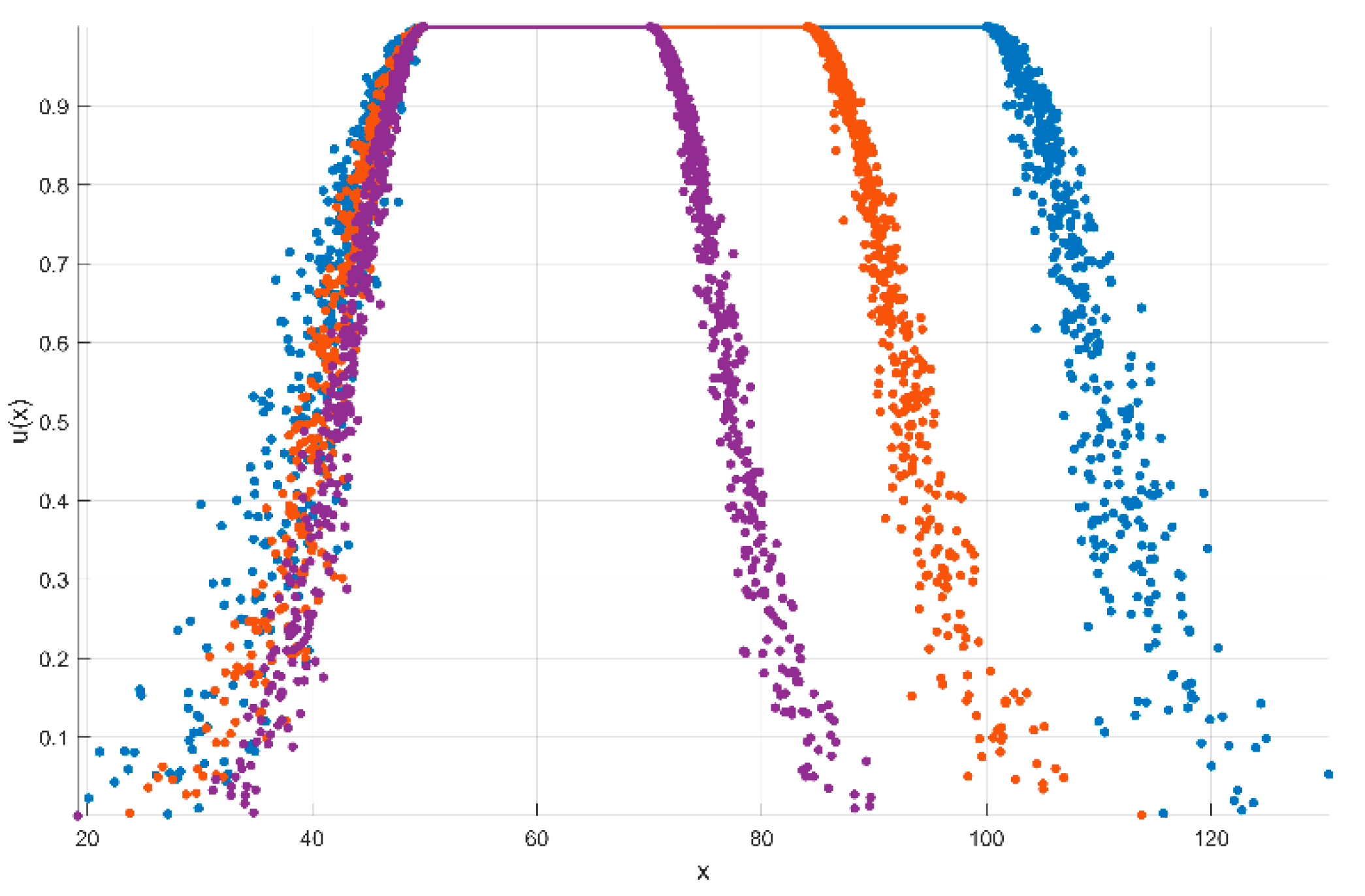
$${\widehat{C}}_{[0,1]}^3=([50,100],9.26,1.97), {\widehat{C}}_{[0,1]}^5=([50,84],8.07,1.12), {\widehat{C}}_{[0,1]}^7=([50,70],6.57,0.81)$$

To present the results more intuitively, the three trapezium clouds in the above example are shown in Figure 3, where the purple trapezium cloud represents ${\widehat{C}}_{[0,1]}^7=([50,70],6.57,0.81)$, the yellow trapezium cloud represents ${\widehat{C}}_{[0,1]}^5=([50,84],8.07,1.12)$, and the blue trapezium cloud represents ${\widehat{C}}_{[0,1]}^3=([50,100],9.26,1.97)$.

4. An Aggregation Method Based on Trapezium Cloud Generalized Weighted Heronian Mean

In this section, the probabilistic uncertain linguistic term set will be extended by introducing the concept of the probabilistic multi-granularity uncertain linguistic term set where linguistic terms are distributed symmetrically. In addition, a method for transforming a probabilistic multi-granularity uncertain linguistic term set into a trapezium cloud that possesses symmetric features will be presented, as well as a method for aggregating multiple trapezium clouds into a single trapezium cloud. When decision-makers have different mental expectations about the given linguistic evaluation information, the traditional linguistic term sets cannot meet such decision-making needs. For this reason, probabilistic linguistic term sets have been proposed. Decision-makers often prefer to provide linguistic evaluation ranges as opposed to individual linguistic evaluation values. As a result, probabilistic uncertain linguistic term sets have been birthed. However, when different decision-makers have different preferences for the granularity of the selected linguistic term set, the probabilistic uncertain linguistic term set cannot provide linguistic term sets with multiple granularities for decision-makers to choose from. Therefore, to address this real-world need, this section extends the probabilistic uncertain linguistic term set by defining probabilistic multi-granularity uncertain linguistic term sets (PMGULTSs) so that linguistic terms are distributed symmetrically.

Definition 7.

A probability multi-granularity uncertain linguistic term set (PMGULTS) can be defined as follows:

$$\tilde{S}(P)=\{<[s_{a_k}^{2t_k+1},s_{b_k}^{2t_k+1}],p_k>|p_k\ge 0,t_k\in \{1,2,\dots ,6\},k=1,2,\dots ,\#\tilde{S}(p),{\displaystyle \sum _{k=1}^{\#\tilde{S}(p)}{p}_k\le 1}\}$$

where$<[s_{a_k}^{2t_k+1},s_{b_k}^{2t_k+1}],p_k>$represents the probabilistic uncertain linguistic term$[s_{a_k}^{2t_k+1},s_{b_k}^{2t_k+1}]$and its probability$p_k$. $s_{a_k}^{2t_k+1 }$and$s_{b_k}^{2t_k+1}$are linguistic terms that from symmetric linguistic term set, where$2t_k+1$is the granularity of the linguistic term,$t_k\in \{1,2,\dots ,6\}$,$s_{a_k}^{2t_k+1}\le s_{b_k}^{2t_k+1}$, and$\#\tilde{S}(p)$is the granularity of$\tilde{S}(p)$.

The formula for transforming a probabilistic multi-granularity uncertain linguistic term set $\tilde{S}(P)$ into a trapezium cloud $\widehat{C}=([\underset{¯}{Ex},\overline{Ex}],En,He)$ is obtained based on the addition and number multiplication operations among trapezium clouds in Definition 6 as follows:

$$\tilde{\gamma }(\tilde{S}(p))=\widehat{C}=([\underset{¯}{Ex},\overline{Ex}],En,He)$$

(7)

where $\underset{¯}{Ex}={\displaystyle \sum _{k=1}^{\#\tilde{S}(p)}{p}_k\underset{¯}{E{x}_{a_k}}}$, $\overline{Ex}={\displaystyle \sum _{k=1}^{\#\tilde{S}(p)}{p}_k\overline{E{x}_{b_k}}}$, $En=\sqrt{{\displaystyle \sum _{k=1}^{\#\tilde{S}(p)}{p}_{k}E{n}_{[a_k,b_k]}^2}}$, $He=\sqrt{{\displaystyle \sum _{k=1}^{\#\tilde{S}(p)}{p}_{k}H{e}_{[a_k,b_k]}^2}}$.

According to Equation (7), the probabilistic uncertain linguistic terms from multiple granularities are transformed into trapezium clouds within the same granularity, i.e., the same universe of discourse.

The Heronian mean is a widely used aggregating method that has been favored by many scholars because of its ability to capture the interrelationships between attributes [44]. Additionally, it is uniquely suited for trapezium cloud aggregation, and the core reason lies in its natural alignment with two key characteristics of standing timber evaluation and trapezium cloud information. (1) Captures attribute correlations: Unlike independent aggregation operators (e.g., weighted arithmetic mean), the Heronian mean inherently considers interactions between attributes. For standing timber evaluation, this means it can reflect real-world correlations, such as diameter at breast height affecting length, avoiding information distortion caused by ignoring attribute links. (2) Adapts to interval uncertainty of trapezium clouds: Trapezium clouds are characterized by interval-valued expectation, and the Heronian mean’s calculation logic can naturally integrate interval information. It avoids the interval information loss risk of other operators, ensuring the aggregated result still retains the uncertainty characteristics of trapezium clouds. Let ${\widehat{C}}_i=([{\underset{¯}{Ex}}_{(i)},{\overline{Ex}}_{(i)}],E{n}_{(i)},H{e}_{(i)}),(i=1,\dots ,n)$ be $n$ trapezium clouds. Substituting the addition and multiplication operations between the trapezium clouds in Definition 6 into the generalized weighted Heronian mean, these $n$ trapezium clouds are aggregated into a single trapezium cloud $\widehat{C}=([\underset{¯}{Ex},\overline{Ex}],En,He)$, where $En$ is calculated as follows:

$$En={\left({\displaystyle \frac{1}{{\displaystyle \sum _{i=1}^n{\displaystyle \sum _{j=i}^n{R}_i{R}_j}}}}{\displaystyle \sum _{i=1}^n{\displaystyle \sum _{j=i}^n{R}_i{R}_j\sqrt{\frac{1}{8}p{({\underset{¯}{Ex}}_{(i)}^{p-1}+{\overline{Ex}}_{(i)}^{p-1})}^{2}E{n}_{(i)}^2({\underset{¯}{Ex}}_{(j)}^{2q}+{\overline{Ex}}_{(j)}^{2q})+\frac{1}{8}q{({\underset{¯}{Ex}}_{(j)}^{q-1}+{\overline{Ex}}_{(j)}^{q-1})}^{2}E{n}_{(j)}^2({\underset{¯}{Ex}}_{(i)}^{2p}+{\overline{Ex}}_{(i)}^{2p})}}}\right)}^{{\displaystyle \frac{1}{p+q}}}$$

(8)

Next, Example 2 will be used to illustrate the lack of rationality in the trapezium cloud operation rule in Definition 6.

Example 2.

Let the entropy of six trapezium clouds be 0.64, 0.77, 0.81, 0.76, 0.77, and 0.8. For the sake of generality, assuming that these six trapezium clouds have the same degree of importance, the entropy of the trapezium clouds is aggregated using Equation (8) when$p=q=1$. The result is 2.8254, which is beyond the original entropy range and easily leads to the distortion of information in the subsequent information aggregation process, which adversely affects the decision-making results.

Therefore, a new trapezium cloud multiplication operation rule is designed to better fit the computational characteristics of the decision model proposed in this study as follows:

Definition 8.

Let ${\widehat{C}}_1=([{\underset{¯}{Ex}}_{(1)},{\overline{Ex}}_{(1)}],E{n}_{(1)},H{e}_{(1)})$ and ${\widehat{C}}_2=([{\underset{¯}{Ex}}_{(2)},{\overline{Ex}}_{(2)}],E{n}_{(2)},H{e}_{(2)})$ be two trapezium clouds. The multiplication operation between trapezium clouds${\widehat{C}}_1$and ${\widehat{C}}_2$ can be defined as:

$${\widehat{C}}_1\otimes {\widehat{C}}_2=([{\underset{¯}{Ex}}_{(1)}{\underset{¯}{Ex}}_{(2)},{\overline{Ex}}_{(1)}{\overline{Ex}}_{(2)}],E{n}_{(1)}E{n}_{(2)},H{e}_{(1)}H{e}_{(2)})$$

(9)

The new multiplication operation and the addition, number multiplication, and power operation in Definition 6 are jointly applied to the generalized weighted Heronian mean, and the calculation method of $En$ is also obtained. Additionally, in order to verify its rationality, it is applied to Example 2, and the aggregation result is $En=0.7586$, which is within the range of the original data, which guarantees the rationality of the subsequent information aggregation results and the scientificity of the decision-making results.

To underscore the novelty of the proposed trapezium cloud generalized weighted Heronian mean, we compare it with two widely used trapezium cloud aggregation operators from different perspectives. First, we compared it with the trapezium cloud weighted averaging (TCWA) operator. The TCWA operator assumes all attributes are independent and achieves aggregation through a simple weighted sum. This design completely ignores correlations between attributes. In contrast, the TCGWHM proactively captures multi-attribute correlations, effectively avoiding this flaw. Second, we compared it with the trapezium cloud weighted Bonferroni averaging (TCWBA) operator. While the TCWBA operator can capture attribute correlations via Bonferroni parameters, its capability is limited to pairwise attribute interactions. It cannot handle multi-indicator correlation scenarios in standing timber evaluation. Moreover, the TCWBA operator relies on fixed parameter settings, lacking flexibility to adapt to indicators with varying uncertainty levels. The TCGWHM addresses these limitations. It captures multi-attribute correlations and supports flexible adjustment of parameters. In summary, the TCGWHM outperforms both the TCWA and TCWBA operators in terms of the range of attribute correlations captured and flexibility in adapting to uncertainty, making it more suitable for the complex scenarios of standing timber evaluation.

Inspired by Peng et al. [20], who introduced the Heronian mean into the process of aggregating probabilistic linguistic terms clouds, the Heronian mean is extended to the process of trapezium cloud information aggregation in this study, and the trapezium cloud generalized weighted Heronian mean ($TCGWHM$) is proposed as follows:

Definition 9.

Let${\widehat{C}}_i=([{\underset{¯}{Ex}}_{(i)},{\overline{Ex}}_{(i)}],E{n}_{(i)},H{e}_{(i)}),(i=1,\dots ,n)$be the set of trapezium clouds, denoted by $\mathrm{\Omega }$. For any $p, q\ge 0$, $TCGWH{M}^{p,q}$ is a mapping $TCGWH{M}^{p,q}:{\mathrm{\Omega }}^n\to \mathrm{\Omega }$ defined as:

$$\begin{array}{l}TCGWH{M}^{p,q}({\widehat{C}}_1,{\widehat{C}}_2,\dots ,{\widehat{C}}_n)=\hfill \\ ([{({\displaystyle \frac{1}{{\displaystyle \sum _{i=1}^n{\displaystyle \sum _{j=i}^n{R}_i{R}_j}}}}{\displaystyle \sum _{i=1}^n{\displaystyle \sum _{j=i}^n{R}_i{R}_j{\underset{¯}{Ex}}_{(i)}^p}}{\underset{¯}{Ex}}_{(j)}^q)}^{{\displaystyle \frac{1}{p+q}}},{({\displaystyle \frac{1}{{\displaystyle \sum _{i=1}^n{\displaystyle \sum _{j=i}^n{R}_i{R}_j}}}}{\displaystyle \sum _{i=1}^n{\displaystyle \sum _{j=i}^n{R}_i{R}_j{\overline{Ex}}_{(i)}^p}}{\overline{Ex}}_{(j)}^q)}^{{\displaystyle \frac{1}{p+q}}}],\hfill \\ {({\displaystyle \frac{1}{{\displaystyle \sum _{i=1}^n{\displaystyle \sum _{j=i}^n{R}_i{R}_j}}}}{\displaystyle \sum _{i=1}^n{\displaystyle \sum _{j=i}^n{R}_i{R}_j}}{\displaystyle \frac{1}{4}}\sqrt{p}\sqrt{q}E{n}_{(i)}E{n}_{(j)}({\underset{¯}{Ex}}_{(i)}^{p-1}+{\overline{Ex}}_{(i)}^{p-1})({\underset{¯}{Ex}}_{(j)}^{q-1}+{\overline{Ex}}_{(j)}^{q-1}))}^{{\displaystyle \frac{1}{p+q}}},\hfill \\ {({\displaystyle \frac{1}{{\displaystyle \sum _{i=1}^n{\displaystyle \sum _{j=i}^n{R}_i{R}_j}}}}{\displaystyle \sum _{i=1}^n{\displaystyle \sum _{j=i}^n{R}_i{R}_j}}{\displaystyle \frac{1}{4}}\sqrt{p}\sqrt{q}H{e}_{(i)}H{e}_{(j)}({\underset{¯}{Ex}}_{(i)}^{p-1}+{\overline{Ex}}_{(i)}^{p-1})({\underset{¯}{Ex}}_{(j)}^{q-1}+{\overline{Ex}}_{(j)}^{q-1}))}^{{\displaystyle \frac{1}{p+q}}})\hfill \end{array}$$

(10)

where $p$ and $q$ are the parameters, $p>0$, $q>0$, $R_i={\displaystyle \frac{1}{2}}({\omega }_i^{-}+{\omega }_i^{+})$, and $[{\omega }_i^{-},{\omega }_i^{+}]$ is the i-th component of the normalized interval weight vector in Definition 2.

5. A Novel Ranking Method Based on the Approximate Centroid of Trapezium Cloud

After the aggregation process, a judgment needs to be made about the superiority or inferiority of the aggregated trapezium cloud. The centroid is the central location of an object’s mass, and in geometric figures, it is usually assumed that its mass is uniformly distributed to find the coordinates of the centroid. Ranking using the centroid has many advantages, such as clear ideas, concise steps, and being simple and easy to operate. Therefore, it is favored by scholars among many ranking methods. Jiao et al. [45] defined the cloud centroid coordinates $(x_0,y_0)$, where $x_0=Ex$, and $y_0$ is related to the indicator weights. Most of the subsequent studies on cloud centroid follow this definition, e.g., that of Wang et al. [46]. Due to the lack of research on the centroid of trapezium clouds, this section derives the calculation formula for the approximate centroid coordinates of trapezium clouds and obtains the sorting method for trapezium clouds based on it.

Compared with traditional ranking methods, the centroid-based ranking method is more suitable for standing timber evaluation. (1) Compared to distance-based method [23]: The distance-based method is highly random, easily losing critical information. In contrast, the centroid-based method comprehensively considers the horizontal and vertical coordinates of the approximate centroid, thereby more steadily and accurately reflecting the relative superiority or inferiority of different alternatives. It also requires no random cloud droplet sampling, ensuring stable results. (2) Compared to the possibility degree method [26]: The possibility degree method fails to handle the scenario when the trapezium cloud degenerates into a cloud, which is common in standing timber evaluation. This will lead to distorted results. In contrast, the centroid-based method can handle this scenario. It also avoids constructing an n × n possibility matrix, simplifying the steps significantly. In summary, the centroid-based ranking method better meets the needs of standing timber evaluation. The following analysis derives the calculation steps for the approximate centroid of the trapezium cloud.

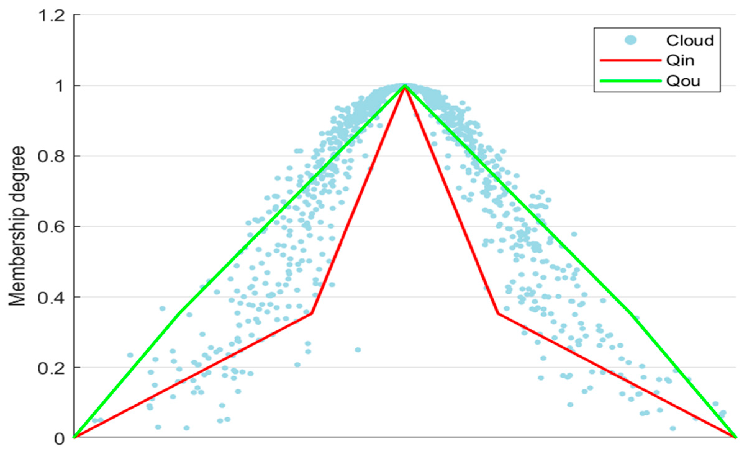
Since the hyper entropy corresponding to the point $(x_0\sqrt{\ln 8}En,{\displaystyle \frac{\sqrt{2}}{4}})$ on the cloud expectation curve reflects the degree of discretization of the cloud according to Li et al. [15], two pentagons $Q_{in}$ and $Q_{ou}$ are extracted from a cloud based on this point as shown in Figure 4.

Let ${\widehat{C}}_i=([{\underset{¯}{Ex}}_{(i)},{\overline{Ex}}_{(i)}],E{n}_{(i)},H{e}_{(i)})$ be a trapezium cloud. The steps for deriving its approximate centroid coordinates are as follows.

Step 1. Calculate the abscissa $x_{{\widehat{C}}_i}$ of the approximate centroid of ${\widehat{C}}_i$:

Since ${\displaystyle \frac{1}{2}}({\overline{Ex}}_{(i)}+{\underset{¯}{Ex}}_{(i)})$ is the most representative value in the abscissa of a trapezium cloud, the abscissa of the approximate centroid of a trapezium cloud is defined as $x_{{\widehat{C}}_i}={\displaystyle \frac{1}{2}}({\overline{Ex}}_{(i)}+{\underset{¯}{Ex}}_{(i)})$.

A trapezium cloud ${\widehat{C}}_i=([{\underset{¯}{Ex}}_{(i)},{\overline{Ex}}_{(i)}],E{n}_{(i)},H{e}_{(i)})$ is considered to have degenerated into a cloud ${\underset{⌣}{C}}_i=({\displaystyle \frac{1}{2}}({\overline{Ex}}_{(i)}+{\underset{¯}{Ex}}_{(i)}),E{n}_{(i)},H{e}_{(i)})$ when the abscissa of the approximate centroid of the trapezium cloud takes the value $x_{{\widehat{C}}_i}={\displaystyle \frac{1}{2}}({\overline{Ex}}_{(i)}+{\underset{¯}{Ex}}_{(i)})$. In this situation, the vertical coordinates of the approximate centroid of cloud ${\underset{⌣}{C}}_i=({\displaystyle \frac{1}{2}}({\overline{Ex}}_{(i)}+{\underset{¯}{Ex}}_{(i)}),E{n}_{(i)},H{e}_{(i)})$ are calculated as the vertical coordinates of the approximate centroid of trapezium cloud ${\widehat{C}}_i=([{\underset{¯}{Ex}}_{(i)},{\overline{Ex}}_{(i)}],E{n}_{(i)},H{e}_{(i)})$.

Step 2. Calculate the vertical coordinates $y_{{\widehat{C}}_i}$ of the approximate centroid of ${\widehat{C}}_i$:

The idea of calculating the vertical coordinates $y_{{\widehat{C}}_i}$ of the approximate centroid of ${\widehat{C}}_i$ is to calculate the average of the vertical coordinates of the centroid of pentagons $Q_{in}$ and $Q_{ou}$.

Step 2.1. Calculate the segmented function equations ${\mu }_{ou}(x)$ and ${\mu }_{in}(x)$ for pentagons $Q_{in}$ and $Q_{ou}$:

Join $(x_{{\widehat{C}}_i}-3E{n}_{(i)},0)$, $(x_{{\widehat{C}}_i}-\sqrt{\ln 8}E{n}_{(i)}-3H{e}_{(i)},{\displaystyle \frac{\sqrt{2}}{4}})$, $(x_{{\widehat{C}}_i},1)$, $(x_{{\widehat{C}}_i}+\sqrt{\ln 8}E{n}_{(i)}+3H{e}_{(i)})$, and $(x_{{\widehat{C}}_i}+3E{n}_{(i)},0)$ in turn to obtain the first pentagon $Q_{ou}$, whose segment function equation is:

$$u_{ou}(x)=\left\{\begin{array}{l}{\displaystyle \frac{\sqrt{2}}{4(3-\sqrt{\ln 8})E{n}_{(i)}-12H{e}_{(i)}}}x-{\displaystyle \frac{\sqrt{2}(x_{{\widehat{C}}_i}-3E{n}_{(i)})}{4(3-\sqrt{\ln 8})E{n}_{(i)}-12H{e}_{(i)}}},x_{{\widehat{C}}_i}-3E{n}_{(i)}\le x<x_{{\widehat{C}}_i}-\sqrt{\ln 8}E{n}_{(i)}-3H{e}_{(i)}\\ {\displaystyle \frac{4-\sqrt{2}}{4(\sqrt{\ln 8}E{n}_{(i)}+3H{e}_{(i)})}}x+{\displaystyle \frac{4(\sqrt{\ln 8}E{n}_{(i)}+3H{e}_{(i)})-(4-\sqrt{2})x_{{\widehat{C}}_i}}{4(\sqrt{\ln 8}E{n}_{(i)}+3H{e}_{(i)})}},x_{{\widehat{C}}_i}-\sqrt{\ln 8}E{n}_{(i)}-3H{e}_{(i)}\le x<x_{{\widehat{C}}_i}\\ {\displaystyle \frac{\sqrt{2}-4}{4(\sqrt{\ln 8}E{n}_{(i)}+3H{e}_{(i)})}}x+{\displaystyle \frac{4(\sqrt{\ln 8}E{n}_{(i)}+3H{e}_{(i)})-(\sqrt{2}-4)x_{{\widehat{C}}_i}}{4(\sqrt{\ln 8}E{n}_{(i)}+3H{e}_{(i)})}},x_{{\widehat{C}}_i}\le x<x_{{\widehat{C}}_i}+\sqrt{\ln 8}E{n}_{(i)}+3H{e}_{(i)}\\ {\displaystyle \frac{-\sqrt{2}}{4(3-\sqrt{\ln 8})E{n}_{(i)}-12H{e}_{(i)}}}x+{\displaystyle \frac{\sqrt{2}(x_{{\widehat{C}}_i}+3E{n}_{(i)})}{4(3-\sqrt{\ln 8})E{n}_{(i)}-12H{e}_{(i)}}},x_{{\widehat{C}}_i}+\sqrt{\ln 8}E{n}_{(i)}+3H{e}_{(i)}\le x<x_{{\widehat{C}}_i}+3E{n}_{(i)}\\ \\ 0,else\end{array}\right.$$

(11)

Similarly, join $(x_{{\widehat{C}}_i}-3E{n}_{(i)},0)$, $(x_{{\widehat{C}}_i}-\sqrt{\ln 8}E{n}_{(i)}+3H{e}_{(i)},{\displaystyle \frac{\sqrt{2}}{4}})$, $(x_{{\widehat{C}}_i},1)$, $(x_{{\widehat{C}}_i}+\sqrt{\ln 8}E{n}_{(i)}-3H{e}_{(i)})$, and $(x_{{\widehat{C}}_i}+3E{n}_{(i)},0)$ in turn to obtain the second pentagon $Q_{in}$, whose segment function equation is:

$$u_{in}(x)=\left\{\begin{array}{l}{\displaystyle \frac{\sqrt{2}}{4(3-\sqrt{\ln 8})E{n}_{(i)}+12H{e}_{(i)}}}x-{\displaystyle \frac{\sqrt{2}(x_{{\widehat{C}}_i}-3E{n}_{(i)})}{4(3-\sqrt{\ln 8})E{n}_{(i)}+12H{e}_{(i)}}},x_{{\widehat{C}}_i}-3E{n}_{(i)}\le x<x_{{\widehat{C}}_i}-\sqrt{\ln 8}E{n}_{(i)}+3H{e}_{(i)}\\ {\displaystyle \frac{4-\sqrt{2}}{4(\sqrt{\ln 8}E{n}_{(i)}-3H{e}_{(i)})}}x+{\displaystyle \frac{4(\sqrt{\ln 8}E{n}_{(i)}-3H{e}_{(i)})-(4-\sqrt{2})x_{{\widehat{C}}_i}}{4(\sqrt{\ln 8}E{n}_{(i)}-3H{e}_{(i)})}},x_{{\widehat{C}}_i}-\sqrt{\ln 8}E{n}_{(i)}+3H{e}_{(i)}\le x<x_{{\widehat{C}}_i}\\ {\displaystyle \frac{\sqrt{2}-4}{4(\sqrt{\ln 8}E{n}_{(i)}-3H{e}_{(i)})}}x+{\displaystyle \frac{4(\sqrt{\ln 8}E{n}_{(i)}-3H{e}_{(i)})-(\sqrt{2}-4)x_{{\widehat{C}}_i}}{4(\sqrt{\ln 8}E{n}_{(i)}-3H{e}_{(i)})}},x_{{\widehat{C}}_i}\le x<x_{{\widehat{C}}_i}+\sqrt{\ln 8}E{n}_{(i)}-3H{e}_{(i)}\\ {\displaystyle \frac{-\sqrt{2}}{4(3-\sqrt{\ln 8})E{n}_{(i)}+12H{e}_{(i)}}}x+{\displaystyle \frac{\sqrt{2}(x_{{\widehat{C}}_i}+3E{n}_{(i)})}{4(3-\sqrt{\ln 8})E{n}_{(i)}+12H{e}_{(i)}}},x_{{\widehat{C}}_i}+\sqrt{\ln 8}E{n}_{(i)}-3H{e}_{(i)}\le x<x_{{\widehat{C}}_i}+3E{n}_{(i)}\\ \\ 0,else\end{array}\right.$$

(12)

Step 2.2. Calculate the vertical coordinate $y_{in}$ of the centroid of $Q_{in}$:

(1). Calculate $g_1^{in}(y_1)$, $g_2^{in}(y_2)$, $g_3^{in}(y_3)$, and $g_4^{in}(y_4)$:

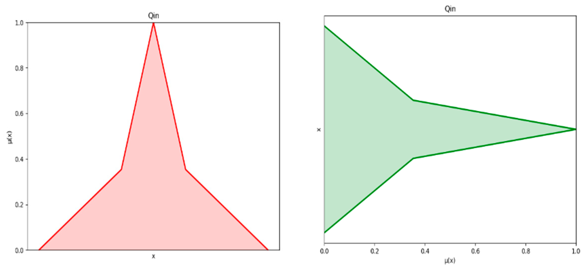
The function graph of $Q_{in}$ and its inverse function graph are shown in Figure 5.

Denoting the four-segment linear function equations in the graph of the inverse function of $Q_{in}$ in a clockwise direction as $g_1^{in}(y_1)$, $g_2^{in}(y_2)$, $g_3^{in}(y_3)$, and $g_4^{in}(y_4)$, they are $g_1^{in}(y_1)=-2\sqrt{2}((3-\sqrt{\ln 8})E{n}_{(i)}+3H{e}_{(i)})y+x_{{\widehat{C}}_i}+3E{n}_{(i)}$, $g_2^{in}(y_2)={\displaystyle \frac{4(\sqrt{\ln 8}E{n}_{(i)}-3H{e}_{(i)})}{\sqrt{2}-4}}y+x_{{\widehat{C}}_i}-{\displaystyle \frac{4(\sqrt{\ln 8}E{n}_{(i)}-3H{e}_{(i)})}{\sqrt{2}-4}}$, $g_3^{in}(y_3)={\displaystyle \frac{4(\sqrt{\ln 8}E{n}_{(i)}-3H{e}_{(i)})}{4-\sqrt{2}}}y+x_{{\widehat{C}}_i}-{\displaystyle \frac{4(\sqrt{\ln 8}E{n}_{(i)}-3H{e}_{(i)})}{4-\sqrt{2}}}$, and $g_4^{in}(y_4)=2\sqrt{2}((3-\sqrt{\ln 8})E{n}_{(i)}+3H{e}_{(i)})y+x_{{\widehat{C}}_i}-3E{n}_{(i)}$ respectively.

(2). Calculate $g_1^{in}+g_2^{in}-g_3^{in}-g_4^{in}$:

$g_1^{in}$, $g_2^{in}$, $g_3^{in}$, and $g_4^{in}$ are the integrals of $g_1^{in}(y_1)$, $g_2^{in}(y_2)$, $g_3^{in}(y_3)$, and $g_4^{in}(y_4)$ in their respective ranges, so

$$g_1^{in}+g_2^{in}-g_3^{in}-g_4^{in}=-{\displaystyle \frac{\sqrt{2}((3-\sqrt{\ln 8})E{n}_{(i)}+3H{e}_{(i)})}{4}}+{\displaystyle \frac{(4\sqrt{2}-9)(\sqrt{\ln 8}-3H{e}_{(i)})}{2(\sqrt{2}-4)}}+{\displaystyle \frac{3\sqrt{2}}{2}}E{n}_{(i)}$$

(3). Calculate $y_1{g}_1^{in}+y_2{g}_2^{in}-y_3{g}_3^{in}-y_4{g}_4^{in}$:

$y_1{g}_1^{in}$, $y_2{g}_2^{in}$, $y_3{g}_3^{in}$, and $y_4{g}_4^{in}$ are the integrals of $y_1{g}_1^{in}(y_1)$, $y_2{g}_2^{in}(y_2)$, $y_3{g}_3^{in}(y_3)$, and $y_4{g}_4^{in}(y_4)$ in their respective ranges, so

$$y_1{g}_1^{in}+y_2{g}_2^{in}-y_3{g}_3^{in}-y_4{g}_4^{in}={\displaystyle \frac{-((3-\sqrt{\ln 8})E{n}_{(i)}+3H{e}_{(i)})}{12}}+{\displaystyle \frac{(10+\sqrt{2})(\sqrt{\ln 8}E{n}_{(i)}-3H{e}_{(i)})}{12(4-\sqrt{2})}}+{\displaystyle \frac{3}{8}}E{n}_{(i)}$$

(4). Calculate the vertical coordinate $y_{in}$ of the centroid of the pentagon $Q_{in}$:

Based on the centroid formula proposed by Wang et al. [47], the formula for the vertical coordinates of the centroid of the pentagon $Q_{in}$ is derived as ${\displaystyle \frac{y_1{g}_1^{in}+y_2{g}_2^{in}-y_3{g}_3^{in}-y_4{g}_4^{in}}{g_1^{in}+g_2^{in}-g_3^{in}-g_4^{in}}}$. Therefore, the vertical coordinate $y_{in}$ of the centroid of $Q_{in}$ is obtained:

$$y_{in}={\displaystyle \frac{-(4-\sqrt{2})((3-\sqrt{\ln 8})E{n}_{(i)}+3H{e}_{(i)})+(10+\sqrt{2})(\sqrt{\ln 8}E{n}_{(i)}-3H{e}_{(i)})}{6(1-2\sqrt{2}((3-\sqrt{\ln 8})E{n}_{(i)}+3H{e}_{(i)})-(4\sqrt{2}-9)(\sqrt{\ln 8}E{n}_{(i)}-3H{e}_{(i)})-6(1-2\sqrt{2})E{n}_{(i)})}}$$

(13)

Step 2.3. Calculate the vertical coordinate $y_{ou}$ of the centroid of $Q_{ou}$:

(1). Calculate $g_1^{ou}(y_1)$, $g_2^{ou}(y_2)$, $g_3^{ou}(y_3)$, and $g_4^{ou}(y_4)$:

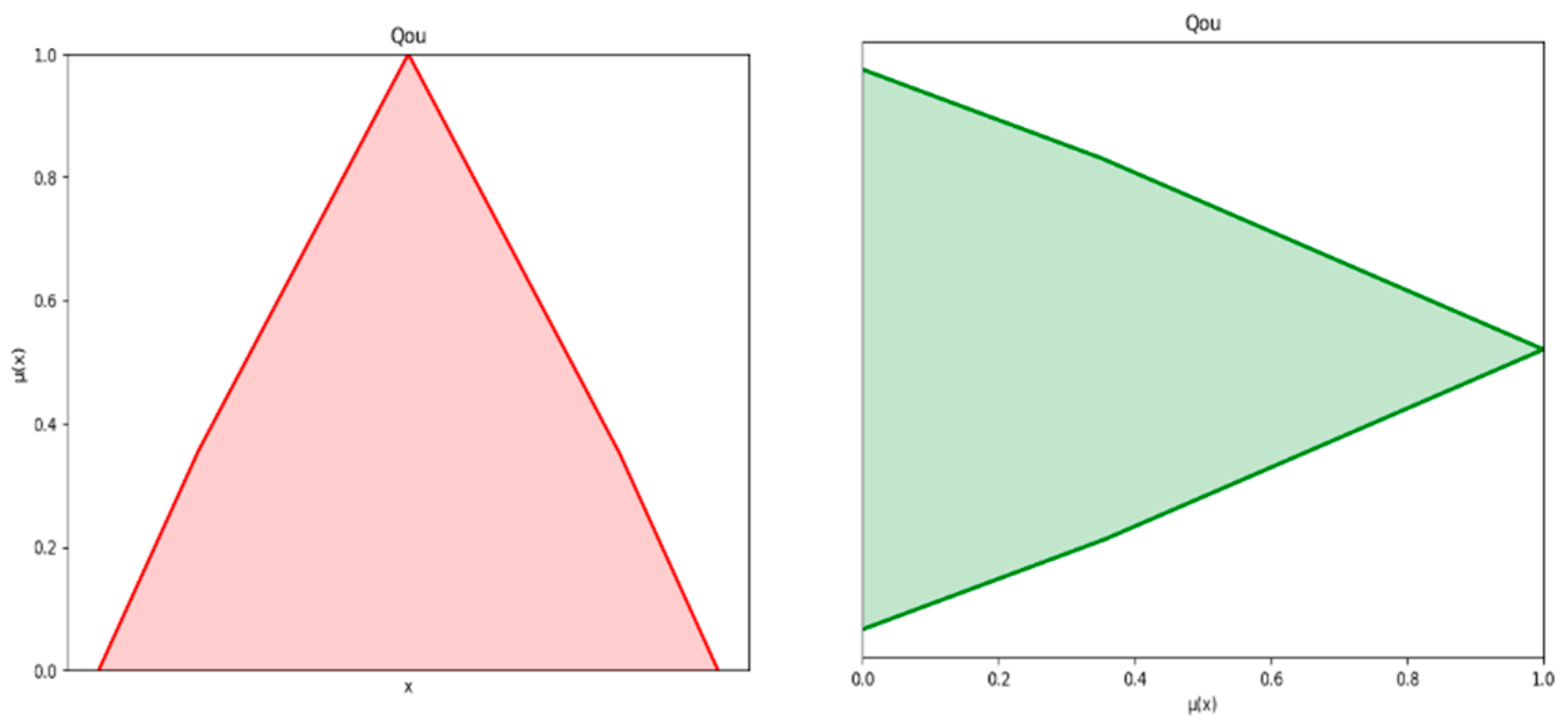
The function graph of $Q_{ou}$ and its inverse function graph are shown in Figure 6.

Denoting the four-segment linear function equations in the graph of the inverse function of $Q_{ou}$ in the clockwise direction as $g_1^{ou}(y_1)$, $g_2^{ou}(y_2)$, $g_3^{ou}(y_3)$, and $g_4^{ou}(y_4)$, they are $g_1^{ou}(y_1)=-2\sqrt{2}((3-\sqrt{\ln 8})E{n}_{(i)}-3H{e}_{(i)})y+x_{{\widehat{C}}_i}+3E{n}_{(i)}$, $g_2^{ou}(y_2)=-{\displaystyle \frac{4(\sqrt{\ln 8}E{n}_{(i)}+3H{e}_{(i)})}{4-\sqrt{2}}}y+x_{{\widehat{C}}_i}+{\displaystyle \frac{4(\sqrt{\ln 8}E{n}_{(i)}+3H{e}_{(i)})}{4-\sqrt{2}}}$, $g_3^{ou}(y_3)={\displaystyle \frac{4(\sqrt{\ln 8}E{n}_{(i)}+3H{e}_{(i)})}{4-\sqrt{2}}}y+x_{{\widehat{C}}_i}-{\displaystyle \frac{4(\sqrt{\ln 8}E{n}_{(i)}+3H{e}_{(i)})}{4-\sqrt{2}}}$, and $g_4^{ou}(y_4)=2\sqrt{2}((3-\sqrt{\ln 8})E{n}_{(i)}-3H{e}_{(i)})y+x_{{\widehat{C}}_i}-3E{n}_{(i)}$, respectively.

(2). Calculate $g_1^{ou}+g_2^{ou}-g_3^{ou}-g_4^{ou}$:

$g_1^{ou}$, $g_2^{ou}$, $g_3^{ou}$, and $g_4^{ou}$ are the integrals of $g_1^{ou}(y_1)$, $g_2^{ou}(y_2)$, $g_3^{ou}(y_3)$, and $g_4^{ou}(y_4)$ in their respective ranges, so

$$g_1^{ou}+g_2^{ou}-g_3^{ou}-g_4^{ou}=-{\displaystyle \frac{\sqrt{2}((3-\sqrt{\ln 8})E{n}_{(i)}-3H{e}_{(i)})}{4}}+{\displaystyle \frac{(9-4\sqrt{2})(\sqrt{\ln 8}E{n}_{(i)}+3H{e}_{(i)})}{2(4-\sqrt{2})}}+{\displaystyle \frac{3\sqrt{2}}{2}}E{n}_{(i)}$$

(3). Calculate $y_1{g}_1^{ou}+y_2{g}_2^{ou}-y_3{g}_3^{ou}-y_4{g}_4^{ou}$:

$y_1{g}_1^{ou}$, $y_2{g}_2^{ou}$, $y_3{g}_3^{ou}$, and $y_4{g}_4^{ou}$ are the integrals of $y_1{g}_1^{ou}(y_1)$, $y_2{g}_2^{ou}(y_2)$, $y_3{g}_3^{ou}(y_3)$, and $y_4{g}_4^{ou}(y_4)$ in their respective ranges, so

$$y_1{g}_1^{ou}+y_2{g}_2^{ou}-y_3{g}_3^{ou}-y_4{g}_4^{ou}={\displaystyle \frac{-((3-\sqrt{\ln 8})E{n}_{(i)}-3H{e}_{(i)})}{12}}+{\displaystyle \frac{(10+\sqrt{2})(\sqrt{\ln 8}E{n}_{(i)}+3H{e}_{(i)})}{12(4-\sqrt{2})}}+{\displaystyle \frac{3}{8}}E{n}_{(i)}$$

(4). Calculate the vertical coordinate $y_{ou}$ of the centroid of the pentagon $Q_{ou}$:

Similarly, based on the centroid formula proposed by Wang et al. [47], the formula for the vertical coordinates of the centroid of the pentagon $Q_{ou}$ is derived as ${\displaystyle \frac{y_1{g}_1^{ou}+y_2{g}_2^{ou}-y_3{g}_3^{ou}-y_4{g}_4^{ou}}{g_1^{ou}+g_2^{ou}-g_3^{ou}-g_4^{ou}}}$. Therefore, the vertical coordinate $y_{ou}$ of the centroid of $Q_{ou}$ is obtained:

$$y_{ou}={\displaystyle \frac{-2(4-\sqrt{2})((3-\sqrt{\ln 8})E{n}_{(i)}-3H{e}_{(i)})+2(10+\sqrt{2})(\sqrt{\ln 8}E{n}_{(i)}+3H{e}_{(i)})+9(4-\sqrt{2})E{n}_{(i)}}{-6(\sqrt{2}(4-\sqrt{2})((3-\sqrt{\ln 8})E{n}_{(i)}-3H{e}_{(i)})+2(9-4\sqrt{2})(\sqrt{\ln 8}E{n}_{(i)}+3H{e}_{(i)})+12(2\sqrt{2}-1)E{n}_{(i)})}}$$

(14)

The arithmetic mean of $y_{in}$ and $y_{ou}$ yields the vertical coordinate $y_{{\widehat{C}}_i}$ of the approximate centroid of the trapezium cloud. In summary, the approximate centroid of a trapezium cloud is defined as follows.

Definition 10.

Let${\widehat{C}}_i=([{\underset{¯}{Ex}}_{(i)},{\overline{Ex}}_{(i)}],E{n}_{(i)},H{e}_{(i)})$be a trapezium cloud. The approximate centroid coordinates of${\widehat{C}}_i$are$\eta ({\widehat{C}}_i)=(x_{{\widehat{C}}_i},y_{{\widehat{C}}_i})$,

$$x_{{\widehat{C}}_i}={\displaystyle \frac{1}{2}}({\overline{Ex}}_{(i)}+{\underset{¯}{Ex}}_{(i)})$$

(15)

$$y_{{\widehat{C}}_i}={\displaystyle \frac{k_{1}E{n}_{(i)}^2-2(1+\frac{\sqrt{2}}{4})k_{2}H{e}_{(i)}^2}{36E{n}_{(i)}^2-k_2^{2}H{e}_{(i)}^2}}$$

(16)

where$k_1=\sqrt{\ln 8}(4+\sqrt{2})\approx 11.256$, $k_2={\displaystyle \frac{(6\sqrt{2}-3+8\sqrt{\ln 8}-2\sqrt{2\ln 8})(\sqrt{2}+4)}{14}}\approx 4.308$.

Remark 3.

When${\underset{¯}{Ex}}_{(i)}={\overline{Ex}}_{(i)}$, trapezium cloud ${\widehat{C}}_i=([{\underset{¯}{Ex}}_{(i)},{\overline{Ex}}_{(i)}],E{n}_{(i)},H{e}_{(i)})$ degenerates into cloud  ${\underset{⌣}{C}}_i=(E{x}_{(i)},E{n}_{(i)},H{e}_{(i)})$. Apparently, at this point, the approximate centroid coordinates of cloud${\underset{⌣}{C}}_i=(E{x}_{(i)},E{n}_{(i)},H{e}_{(i)})$can be calculated as follows:

$$(x_{{\underset{⌣}{C}}_i},y_{{\underset{⌣}{C}}_i})=(E{x}_{(i)},{\displaystyle \frac{2k_1{k}_{3}E{n}_{(i)}^2-2k_2{k}_{4}H{e}_{(i)}^2}{k_3^{2}E{n}_{(i)}^2-k_4^{2}H{e}_{(i)}^2}})$$

(17)

Definition 11.

Let${\widehat{C}}_1=([{\underset{¯}{Ex}}_{(1)},{\overline{Ex}}_{(1)}],E{n}_{(1)},H{e}_{(1)})$and ${\widehat{C}}_2=([{\underset{¯}{Ex}}_{(2)},{\overline{Ex}}_{(2)}],E{n}_{(2)},H{e}_{(2)})$ be two arbitrary trapezium clouds in the same universe of discourse $U$. Then, the centroids of ${\widehat{C}}_1$ and ${\widehat{C}}_2$ are $\eta ({\widehat{C}}_1)$ and $\eta ({\widehat{C}}_2)$, respectively, and the ranking formula$T_i$ ($i=1, 2$) is given as:

$$T_i=x_{{\widehat{C}}_i}{y}_{{\widehat{C}}_i}={\displaystyle \frac{({\overline{Ex}}_{(i)}+{\underset{¯}{Ex}}_{(i)})(6k_{1}E{n}_{(i)}^2-(1+\frac{\sqrt{2}}{4})k_{2}H{e}_{(i)}^2)}{36E{n}_{(i)}^2-k_2^{2}H{e}_{(i)}^2}}$$

(18)

(1). If $T_1>T_2$, then trapezium cloud ${\widehat{C}}_1$ is superior to ${\widehat{C}}_2$, denoted as ${\widehat{C}}_1\succ {\widehat{C}}_2$;

(2). If $T_1<T_2$, then trapezium cloud ${\widehat{C}}_1$ is inferior to ${\widehat{C}}_2$, denoted as ${\widehat{C}}_1\prec {\widehat{C}}_2$;

(3). If $T_1=T_2$, then trapezium cloud ${\widehat{C}}_1$ and ${\widehat{C}}_2$ are neither superior nor inferior, denoted as ${\widehat{C}}_1\sim {\widehat{C}}_2$.

6. The Trapezium Cloud Model-Based Multi-Attribute Decision-Making Method

6.1. The Measure of the Interval Similarity of Trapezium Clouds

The similarity measure between cloud models is an important part of cloud theory and a hot area of research among scholars. Since the birth of cloud theory, many scholars have studied cloud similarity and achieved fruitful research results. According to the different entry points of these methods, they can be roughly categorized into three categories. (1) Based on cloud droplets: Zhang et al. [48] calculated the distance between some random cloud droplets in two clouds in order to get the formula for cloud similarity. (2) Based on three numerical features of clouds: The representative method is LICM [49], which takes the three numerical features of two clouds as vectors and obtains the cloud similarity by calculating the cosine value of the angle between the vectors. (3) Based on cloud curves: Li et al. [50] proposed ECM and MCM. In addition to the above three categories, there are also some new methods proposed based on the above methods, such as by Zhu et al. [51], Guan et al. [52], and so on.

While the research on the similarity between cloud models has yielded fruitful results, there is a paucity of studies on the similarity between trapezium clouds. Chen et al. [23] extended the interval number similarity measure to the trapezium cloud setting and obtained a formula for the similarity of trapezium clouds by using the maximum–minimum operator. Given that the expectation of a trapezium cloud is an interval number, which is inherently characterized by randomness and uncertainty, this directly contributes to the randomness and uncertainty of the trapezium cloud. Therefore, it is natural and logical to use interval similarity, in other words, the form of an interval number, to portray the similarity between two trapezium clouds. The core information form in standing timber quality evaluation is the trapezium cloud. Traditional classical similarity measures (e.g., cosine similarity, Euclidean distance similarity) have inherent limitations in this scenario, while interval similarity is more suitable, with the core reason lying in the matching of information forms. Classical similarity measures are based on single-point values for calculation. For a trapezium cloud in standing timber assessment, they need to first compress the interval expectation into a fixed value. This process directly loses the fluctuation range of interval boundaries and uncertain information, resulting in similarity results that fail to reflect the essential characteristics of the information. In contrast, interval similarity takes the entire interval as the calculation unit, which can simultaneously incorporate key information such as interval upper and lower bounds and span. It is fully consistent with the form of the trapezium cloud, ensuring that no critical information is omitted in the similarity calculation and meeting the requirement of accurately characterizing data characteristics in standing timber evaluation.

In view of this, the present study proposes a novel methodology for obtaining a new trapezium cloud similarity calculation method that is consistent with the trapezium cloud’s characteristics. This method is based on the trapezium cloud’s interval-valued expectation, and it involves projecting the trapezium cloud onto the horizontal axis.

Let ${\widehat{C}}_i=([{\underset{¯}{Ex}}_{(i)},{\overline{Ex}}_{(i)}],E{n}_{(i)},H{e}_{(i)})$ be a trapezium cloud. $[{\underset{¯}{Ex}}_{(i)},{\overline{Ex}}_{(i)}]$ is its expectation interval, where the lower limit ${\underset{¯}{Ex}}_{(i)}$ represents the lower limit of the expectation, which cannot be lower than this value, and the upper limit ${\overline{Ex}}_{(i)}$ represents the upper limit of the expectation, which cannot be higher than this value. Based on Li et al. [50], let $en=En+He$ in $y=\exp \{-{\displaystyle \frac{{(x-Ex)}^2}{2{(En+He)}^2}}\}$. Therefore, in this section, let $e{n}_{(i)}=E{n}_{(i)}+H{e}_{(i)}$. The expectation interval $[{\underset{¯}{Ex}}_{(i)},{\overline{Ex}}_{(i)}]$ is abstracted as a track in which the trapezium cloud glides. The trapezium cloud is projected onto the horizontal axis, thereby obtaining two intervals, $[{\underset{¯}{Ex}}_{(i)}-3e{n}_{(i)},{\underset{¯}{Ex}}_{(i)}+3e{n}_{(i)}]$ and $[{\overline{Ex}}_{(i)}-3e{n}_{(i)},{\overline{Ex}}_{(i)}+3e{n}_{(i)}]$.

Let ${\widehat{C}}_u=([{\underset{¯}{Ex}}_{(u)},{\overline{Ex}}_{(u)}],E{n}_{(u)},H{e}_{(u)})$ and ${\widehat{C}}_h=([{\underset{¯}{Ex}}_{(h)},{\overline{Ex}}_{(h)}],E{n}_{(h)},H{e}_{(h)})$ be two trapezium clouds. For ${\widehat{C}}_u$, the projection yields two intervals $[{\underset{¯}{Ex}}_{(u)}-3e{n}_{(u)},{\underset{¯}{Ex}}_{(u)}+3e{n}_{(u)}]$ and $[{\overline{Ex}}_{(u)}-3e{n}_{(u)},{\overline{Ex}}_{(u)}+3e{n}_{(u)}]$, denoted as $I_{{(u)}_1}$ and $I_{{(u)}_2}$, respectively. For ${\widehat{C}}_h$, similarly, the projection yields two intervals $[{\underset{¯}{Ex}}_{(h)}-3e{n}_{(h)},{\underset{¯}{Ex}}_{(h)}+3e{n}_{(h)}]$ and $[{\overline{Ex}}_{(h)}-3e{n}_{(h)},{\overline{Ex}}_{(h)}+3e{n}_{(h)}]$, denoted as $I_{{(h)}_1}$ and $I_{{(h)}_2}$. Obviously, the widths of the intervals $I_{{(u)}_1}$ and $I_{{(u)}_2}$ are the same, and the width of their intervals is denoted as ${\ddot{l}}_{(u)}$, and in fact ${\ddot{l}}_{(u)}=6e{n}_{(u)}$. Similarly, the interval widths of $I_{{(h)}_1}$ and $I_{{(h)}_2}$ are the same, and the width of their intervals is denoted as ${\ddot{l}}_{(h)}$, ${\ddot{l}}_{(h)}=6e{n}_{(h)}$. Therefore, the interval similarity between trapezium clouds is defined as follows.

Definition 12.

Let${\widehat{C}}_u=([{\underset{¯}{Ex}}_{(u)},{\overline{Ex}}_{(u)}],E{n}_{(u)},H{e}_{(u)})$ and ${\widehat{C}}_h=([{\underset{¯}{Ex}}_{(h)},{\overline{Ex}}_{(h)}],E{n}_{(h)},H{e}_{(h)})$ be two trapezium clouds. Then, the interval similarity between${\widehat{C}}_u$and${\widehat{C}}_h$can be measured as follows:

$$si{m}_{[{\widehat{C}}_u,{\widehat{C}}_h]}=[si{m}_{\min }({\widehat{C}}_u,{\widehat{C}}_h),si{m}_{\max }({\widehat{C}}_u,{\widehat{C}}_h)]$$

(19)

where$si{m}_{\min }({\widehat{C}}_u,{\widehat{C}}_h)=\sqrt{{\displaystyle \frac{\underset{g,r\in \{1,2\}}{\min }\{\stackrel{⌣}{l}(I_{{(u)}_g},I_{{(h)}_r})\}}{3(e{n}_{(u)}+e{n}_{(h)})}}}$is the lower limit of interval similarity,$si{m}_{\max }({\widehat{C}}_u,{\widehat{C}}_h)=\sqrt{{\displaystyle \frac{\underset{g,r\in \{1,2\}}{\max }\{\stackrel{⌣}{l}(I_{{(u)}_g},I_{{(h)}_r})\}}{3(e{n}_{(u)}+e{n}_{(h)})}}}$is the upper limit of interval similarity, and$\underset{g,r\in \{1,2\}}{\stackrel{⌣}{l}}(I_{{(u)}_g},I_{{(h)}_r})$is the width of the intersecting parts of the intervals.

Property 4.

$si{m}_{\min }({\widehat{C}}_u,{\widehat{C}}_h)\ge 0$, $si{m}_{\max }({\widehat{C}}_u,{\widehat{C}}_h)\le 1$, and $[0,0]\le si{m}_{[{\widehat{C}}_u,{\widehat{C}}_h]}\le [1,1]$, and for trapezium clouds${\widehat{C}}_u$and${\widehat{C}}_h$, $si{m}_{\max }({\widehat{C}}_u,{\widehat{C}}_h)\ge si{m}_{\min }({\widehat{C}}_u,{\widehat{C}}_h)$.

Proof. 

Since $si{m}_{\min }({\widehat{C}}_u,{\widehat{C}}_h)=\sqrt{{\displaystyle \frac{\underset{g,r\in \{1,2\}}{\min }\{\stackrel{⌣}{l}(I_{{(u)}_g},I_{{(h)}_r})\}}{3(e{n}_{(u)}+e{n}_{(h)})}}}$, ${\displaystyle \frac{1}{3}}>0$, $e{n}_{(u)}+e{n}_{(h)}>0$, and $\underset{g,r\in \{1,2\}}{\stackrel{⌣}{l}}(I_{{(u)}_g},I_{{(h)}_r})\ge 0$, so $si{m}_{\min }({\widehat{C}}_u,{\widehat{C}}_h)\ge 0$.

Since $si{m}_{\max }({\widehat{C}}_u,{\widehat{C}}_h)=\sqrt{{\displaystyle \frac{\underset{g,r\in \{1,2\}}{\max }\{\stackrel{⌣}{l}(I_{{(u)}_g},I_{{(h)}_r})\}}{3(e{n}_{(u)}+e{n}_{(h)})}}}$, and obviously when $\underset{g,r\in \{1,2\}}{\max }\{\stackrel{⌣}{l}(I_{{(u)}_g},I_{{(h)}_r})\}=3(e{n}_{(u)}+e{n}_{(h)})$, the maximum value is taken to be 1, then $si{m}_{\max }({\widehat{C}}_u,{\widehat{C}}_h)\le 1$. Since $si{m}_{\min }({\widehat{C}}_u,{\widehat{C}}_h)=\sqrt{{\displaystyle \frac{\underset{g,r\in \{1,2\}}{\min }\{\stackrel{⌣}{l}(I_{{(u)}_g},I_{{(h)}_r})\}}{3(e{n}_{(u)}+e{n}_{(h)})}}}$ and $si{m}_{\max }({\widehat{C}}_u,{\widehat{C}}_h)=\sqrt{{\displaystyle \frac{\underset{g,r\in \{1,2\}}{\max }\{\stackrel{⌣}{l}(I_{{(u)}_g},I_{{(h)}_r})\}}{3(e{n}_{(u)}+e{n}_{(h)})}}}$, then $si{m}_{\max }({\widehat{C}}_u,{\widehat{C}}_h)\ge si{m}_{\min }({\widehat{C}}_u,{\widehat{C}}_h)$, and when $\underset{g,r\in \{1,2\}}{\stackrel{⌣}{l}}(I_{{(u)}_g},I_{{(h)}_r})=0$, the equal sign holds. Thus, for trapezium clouds ${\widehat{C}}_u$ and ${\widehat{C}}_h$, $si{m}_{\max }({\widehat{C}}_u,{\widehat{C}}_h)\ge si{m}_{\min }({\widehat{C}}_u,{\widehat{C}}_h)$ holds. Therefore, $[0,0]\le si{m}_{[{\widehat{C}}_u,{\widehat{C}}_h]}\le [1,1]$ holds. □

Property 5.

When${\widehat{C}}_u={\widehat{C}}_h$, $si{m}_{\max }({\widehat{C}}_u,{\widehat{C}}_h)=1$; when ${\underset{¯}{Ex}}_{(u)}={\overline{Ex}}_{(u)}={\underset{¯}{Ex}}_{(h)}={\overline{Ex}}_{(h)}=Ex$ and $e{n}_{(u)}=e{n}_{(h)}$,$si{m}_{\min }({\widehat{C}}_u,{\widehat{C}}_h)=1$.

Proof. 

When ${\widehat{C}}_u={\widehat{C}}_h$, $I_{{(u)}_1}$ or $I_{{(u)}_2}$ is the same as $I_{{(h)}_1}$ or $I_{{(h)}_2}$, namely $\underset{g,r\in \{1,2\}}{\max }\{\stackrel{⌣}{l}(I_{{(u)}_g},I_{{(h)}_r})\}=3(e{n}_{(u)}+e{n}_{(h)})$, so $si{m}_{\max }({\widehat{C}}_u,{\widehat{C}}_h)=1$. In particular, since $I_{{(u)}_1}$, $I_{{(u)}_2}$, $I_{{(h)}_1}$, and $I_{{(h)}_2}$ are equal when ${\underset{¯}{Ex}}_{(u)}={\overline{Ex}}_{(u)}={\underset{¯}{Ex}}_{(h)}={\overline{Ex}}_{(h)}=Ex$ and $e{n}_{(u)}=e{n}_{(h)}$, then $\stackrel{⌣}{l}(I_{{(u)}_1},I_{{(h)}_1})=\stackrel{⌣}{l}(I_{{(u)}_1},I_{{(h)}_2})=\stackrel{⌣}{l}(I_{{(u)}_2},I_{{(h)}_1})=\stackrel{⌣}{l}(I_{{(u)}_2},I_{{(h)}_2})=3(e{n}_{(u)}+e{n}_{(h)})$. Thus, $si{m}_{\min }({\widehat{C}}_u,{\widehat{C}}_h)=1$ holds. □

Property 6.

$si{m}_{[{\widehat{C}}_u,{\widehat{C}}_h]}=si{m}_{[{\widehat{C}}_h,{\widehat{C}}_u]}$.

Proof. 

$si{m}_{[{\widehat{C}}_u,{\widehat{C}}_h]}=[si{m}_{\min }({\widehat{C}}_u,{\widehat{C}}_h),si{m}_{\max }({\widehat{C}}_u,{\widehat{C}}_h)]$, $si{m}_{\min }({\widehat{C}}_u,{\widehat{C}}_h)=\sqrt{{\displaystyle \frac{\underset{g,r\in \{1,2\}}{\min }\{\stackrel{⌣}{l}(I_{{(u)}_g},I_{{(h)}_r})\}}{3(e{n}_{(u)}+e{n}_{(h)})}}}$, $si{m}_{\max }({\widehat{C}}_u,{\widehat{C}}_h)=\sqrt{{\displaystyle \frac{\underset{g,r\in \{1,2\}}{\max }\{\stackrel{⌣}{l}(I_{{(u)}_g},I_{{(h)}_r})\}}{3(e{n}_{(u)}+e{n}_{(h)})}}}$. $si{m}_{[{\widehat{C}}_h,{\widehat{C}}_u]}=[si{m}_{\min }({\widehat{C}}_h,{\widehat{C}}_u),si{m}_{\max }({\widehat{C}}_h,{\widehat{C}}_u)]$, $si{m}_{\min }({\widehat{C}}_h,{\widehat{C}}_u)=\sqrt{{\displaystyle \frac{\underset{g,r\in \{1,2\}}{\min }\{\stackrel{⌣}{l}(I_{{(h)}_g},I_{{(u)}_r})\}}{3(e{n}_{(u)}+e{n}_{(h)})}}}$, $si{m}_{\max }({\widehat{C}}_h,{\widehat{C}}_u)=\sqrt{{\displaystyle \frac{\underset{g,r\in \{1,2\}}{\max }\{\stackrel{⌣}{l}(I_{{(h)}_g},I_{{(u)}_r})\}}{3(e{n}_{(u)}+e{n}_{(h)})}}}$. Obviously, the only difference between measure $si{m}_{[{\widehat{C}}_u,{\widehat{C}}_h]}$ and measure $si{m}_{[{\widehat{C}}_h,{\widehat{C}}_u]}$ is that for measure $si{m}_{[{\widehat{C}}_u,{\widehat{C}}_h]}$, $I_{{(u)}_1}$ and $I_{{(u)}_2}$ are derived first, and $I_{{(h)}_1}$ and $I_{{(h)}_2}$ are derived later, whereas for measure $si{m}_{[{\widehat{C}}_h,{\widehat{C}}_u]}$, $I_{{(u)}_1}$ and $I_{{(u)}_2}$ are derived later, and $I_{{(h)}_1}$ and $I_{{(h)}_2}$ are derived first, but this makes no difference computationally. Namely, $si{m}_{\min }({\widehat{C}}_u,{\widehat{C}}_h)=si{m}_{\min }({\widehat{C}}_h,{\widehat{C}}_u)$, and $si{m}_{\max }({\widehat{C}}_u,{\widehat{C}}_h)=si{m}_{\max }({\widehat{C}}_h,{\widehat{C}}_u)$. Therefore, $si{m}_{[{\widehat{C}}_u,{\widehat{C}}_h]}=si{m}_{[{\widehat{C}}_h,{\widehat{C}}_u]}$ holds. □

According to Property 5, when two trapezium clouds ${\widehat{C}}_u$ and ${\widehat{C}}_h$ have identical numerical features, namely ${\underset{¯}{Ex}}_{(u)}={\underset{¯}{Ex}}_{(h)}$, ${\overline{Ex}}_{(u)}={\overline{Ex}}_{(h)}$, $E{n}_{(u)}=E{n}_{(h)}$, and $H{e}_{(u)}=H{e}_{(h)}$, the upper limit of the interval similarity between ${\widehat{C}}_u$ and ${\widehat{C}}_h$ is taken to be 1, i.e., $si{m}_{\max }({\widehat{C}}_u,{\widehat{C}}_h)=1$, while the lower limit is not necessarily taken to be 1, i.e., $si{m}_{\min }({\widehat{C}}_u,{\widehat{C}}_h)\le 1$, i.e., $si{m}_{[{\widehat{C}}_u,{\widehat{C}}_h]}=[\le 1,1]$ rather than $si{m}_{[{\widehat{C}}_u,{\widehat{C}}_h]}=[1,1]=1$. This is reasonable, and it demonstrates that the concept of interval similarity proposed in this study takes into account the fuzziness and uncertainty in the trapezium cloud caused by the expectation interval.

6.2. Derive the Normalized Interval Weights of Attributes from the Interval Similarity

It is more natural and logical to use normalized interval weights to characterize fuzziness and uncertainty than to use real weights. Therefore, this section introduces a method for deriving attribute normalized interval weights based on the interval similarity between trapezium clouds by building an optimization model.

The core of standing timber quality evaluation lies in quantifying the importance of each indicator through attribute weights. However, the evaluation data exists in the form of trapezium clouds, which inherently possess the characteristic of uncertainty. Traditional weight calculation models (such as AHP and the entropy weight method) take single-point data as the input and need to compress attribute intervals into fixed values. This leads to the loss of uncertainty information. Furthermore, the weights obtained by traditional models are mostly deterministic values, which cannot reflect the impact of evaluation value interval fluctuations on weights. Based on this, this study constructs the attribute normalized interval weight optimization model based on interval similarity. Its core motivation is to incorporate the uncertainty into the weight calculation process, which provides more accurate weight support for standing timber evaluation. The following elaborates on the construction of the attribute normalized interval weight optimization model based on interval similarity.

Let there be $m$ alternatives $A_i$ and $n$ attributes $B_j$. The trapezium cloud obtained under attribute $B_j$ with respect to alternative $A_i$ is denoted as ${\widehat{C}}_{ij}=([{\underset{¯}{Ex}}_{(ij)},{\overline{Ex}}_{(ij)}],E{n}_{(ij)},H{e}_{(ij)})$. According to the theory in Section 6.1, $e{n}_{(ij)}=E{n}_{(ij)}+H{e}_{(ij)}$. The normalized interval weight of attribute $B_j$ is ${\tilde{\omega }}_j=[{\omega }_j^{-},{\omega }_j^{+}]$, and solving for ${\tilde{\omega }}_j$ requires firstly solving the established bi-objective optimization model and secondly solving the single-objective optimization model converted from the bi-objective optimization model. If the evaluation information obtained by each alternative under a certain attribute, i.e., a trapezium cloud, has a high interval similarity between them, it is considered that the attribute does not play a sufficient role in distinguishing the superiority or inferiority of the alternatives and is given a smaller weight. Based on this view, the optimization model is constructed as follows.

(M-1):

$$\begin{array}{l}\min Z_1={\displaystyle \sum _{j=1}^n{\displaystyle \sum _{i=1}^m{\displaystyle \sum _{k=i+1}^m{({\omega }_j^{-}\sqrt{\frac{\underset{g,r\in \{1,2\}}{\min }\{\stackrel{⌣}{l}(I_{{(ij)}_g},I_{{(kj)}_r})\}}{3(e{n}_{(ij)}+e{n}_{(kj)})}})}^2}}}\\ \min Z_2={\displaystyle \sum _{j=1}^n{\displaystyle \sum _{i=1}^m{\displaystyle \sum _{k=i+1}^m{({\omega }_j^{+}\sqrt{\frac{\underset{g,r\in \{1,2\}}{\max }\{\stackrel{⌣}{l}(I_{{(ij)}_g},I_{{(kj)}_r})\}}{3(e{n}_{(ij)}+e{n}_{(kj)})}})}^2}}}\\ s.t.\left\{\begin{array}{l}{\omega }_p^{-}+{\displaystyle \sum _{\begin{array}{l}j=1\\ j\ne p\end{array}}^n{\omega }_j^{+}\ge 1,p=1,\dots ,n}\\ {\omega }_p^{+}+{\displaystyle \sum _{\begin{array}{l}j=1\\ j\ne p\end{array}}^n{\omega }_j^{-}\le 1,p=1,\dots ,n}\\ {\omega }_j^{+}\ge {\omega }_j^{-},j=1,\dots ,n\\ {\omega }_j^{+},{\omega }_j^{-}\ge 0,j=1,\dots ,n\end{array}\right. \end{array}$$

where ${\omega }_p^{-}+{\displaystyle \sum _{\begin{array}{l}j=1\\ j\ne p\end{array}}^n{\omega }_j^{+}\ge 1}$, ${\omega }_p^{+}+{\displaystyle \sum _{\begin{array}{l}j=1\\ j\ne p\end{array}}^n{\omega }_j^{-}\le 1}$, and $p=1,\dots ,n$ is the inequality condition for solving the normalized interval weights proposed by Sugihara et al. [39].

Due to the large computational volume and high difficulty of solving the multi-objective optimization problem, it increases the computational complexity and reduces the computational efficiency of the model. Therefore, inspired by Yesmin and Alim [53], the above bi-objective optimization model is transformed into a single-objective optimization model for the solution using a new transformation method as follows.

(M-2):

$$\begin{array}{l}\min Z={\displaystyle \frac{{\displaystyle \sum _{j=1}^n{\displaystyle \sum _{i=1}^m{\displaystyle \sum _{k=i+1}^m{({\omega }_j^{-}\sqrt{\frac{\underset{g,r\in \{1,2\}}{\min }\{\stackrel{⌣}{l}(I_{{(ij)}_g},I_{{(kj)}_r})\}}{3(e{n}_{(ij)}+e{n}_{(kj)})}})}^2}}}}{e^{\max \{{\varphi }_1,\frac{1}{2}({\varphi }_1+{\varphi }_2)\}}}}+{\displaystyle \frac{{\displaystyle \sum _{j=1}^n{\displaystyle \sum _{i=1}^m{\displaystyle \sum _{k=i+1}^m{({\omega }_j^{+}\sqrt{\frac{\underset{g,r\in \{1,2\}}{\max }\{\stackrel{⌣}{l}(I_{{(ij)}_g},I_{{(kj)}_r})\}}{3(e{n}_{(ij)}+e{n}_{(kj)})}})}^2}}}}{e^{\max \{{\varphi }_2,\frac{1}{2}({\varphi }_1+{\varphi }_2)\}}}}\\ s.t.\left\{\begin{array}{l}{\omega }_p^{-}+{\displaystyle \sum _{\begin{array}{l}j=1\\ j\ne p\end{array}}^n{\omega }_j^{+}\ge 1,p=1,\dots ,n}\\ {\omega }_p^{+}+{\displaystyle \sum _{\begin{array}{l}j=1\\ j\ne p\end{array}}^n{\omega }_j^{-}\le 1,p=1,\dots ,n}\\ {\omega }_j^{+}\ge {\omega }_j^{-},j=1,\dots ,n\\ {\omega }_j^{+},{\omega }_j^{-}\ge 0,j=1,\dots ,n\end{array}\right. \end{array}$$

where $\min Z_1={\varphi }_1$, and $\min Z_2={\varphi }_2$.

6.3. The Steps of the Proposed Trapezium Cloud Multi-Attribute Decision-Making Model

Let $A=\{A_1,A_2,\dots ,A_m\}$ be a finite set of $m$ alternatives and $B=\{B_1,B_2,\dots B_n\}$ be the set of $n$ attributes whose normalized interval weight vector is $\tilde{\omega }=\left({\tilde{\omega }}_1,{\tilde{\omega }}_2,\dots ,{\tilde{\omega }}_n\right)$. The notions $A_i(i=1,2,\dots ,m)$ and $B_j(j=1,2,\dots ,n)$ respectively represent the $i$th alternative and $j$th attribute. The trapezium cloud about the alternative $A_i$ obtained under the attribute $B_j$ is denoted as ${\widehat{C}}_{ij}=([{\underset{¯}{Ex}}_{(ij)},{\overline{Ex}}_{(ij)}],E{n}_{(ij)},H{e}_{(ij)})$. A trapezium cloud multi-attribute decision-making (TCMADM) model is established based on the previous analysis and discussion. Moreover, the details of the trapezium cloud decision-making model are described in the following steps:

Step 1. Collect information to obtain the probabilistic uncertain linguistic terms of alternative $A_i(i=1,2,\dots ,m)$ under attribute $B_j(j=1,2,\dots ,n)$ from which the probabilistic multi-granularity uncertain linguistic term set $\tilde{S}{(P)}_{ij},i\in \{1,2,\dots ,m\};j\in \{1,2,\dots ,n\}$ is obtained and based on which the probabilistic multi-granularity uncertain linguistic decision matrix $\overline{\mathrm{{\rm M}}}$ is constructed.

Step 2. According to Equations (6) and (7), the probabilistic multi-granularity uncertain linguistic decision matrix $\overline{\mathrm{{\rm M}}}$ is transformed into the trapezium cloud decision matrix $\widetilde{\mathrm{{\rm M}}}$.

Step 3. The interval similarity

$$si{m}_{[{\widehat{C}}_{ij},{\widehat{C}}_{kj}]}=[si{m}_{\min }({\widehat{C}}_{ij},{\widehat{C}}_{kj}),si{m}_{\max }({\widehat{C}}_{ij},{\widehat{C}}_{kj})],i=1,\dots ,m;k=i+1,\dots ,m;j=1,\dots ,n$$

between trapezium clouds is calculated using Equation (19), based on which the normalized interval weights ${\tilde{\omega }}_j=[{\omega }_j^{-},{\omega }_j^{+}],j=1,\dots ,n$ of the attributes in the trapezium cloud decision matrix are obtained by solving (M-1) and (M-2).

Step 4. The trapezium clouds in the decision matrix are aggregated using Equation (10) to obtain the integrated trapezium cloud vector $V$.

Step 5. Calculate the approximate centroid $\eta ({\widehat{C}}_i)=(x_{{\widehat{C}}_i},y_{{\widehat{C}}_i}),i=1,\dots ,m$ of the integrated trapezium cloud represented by alternative $A_i,i=1,\dots ,m$ using Equations (15) and (16).

Step 6. Alternative $A_i, i=1,\dots ,m$ is ranked according to the value of $T_i,i=1,\dots ,m$ by Equation (18).

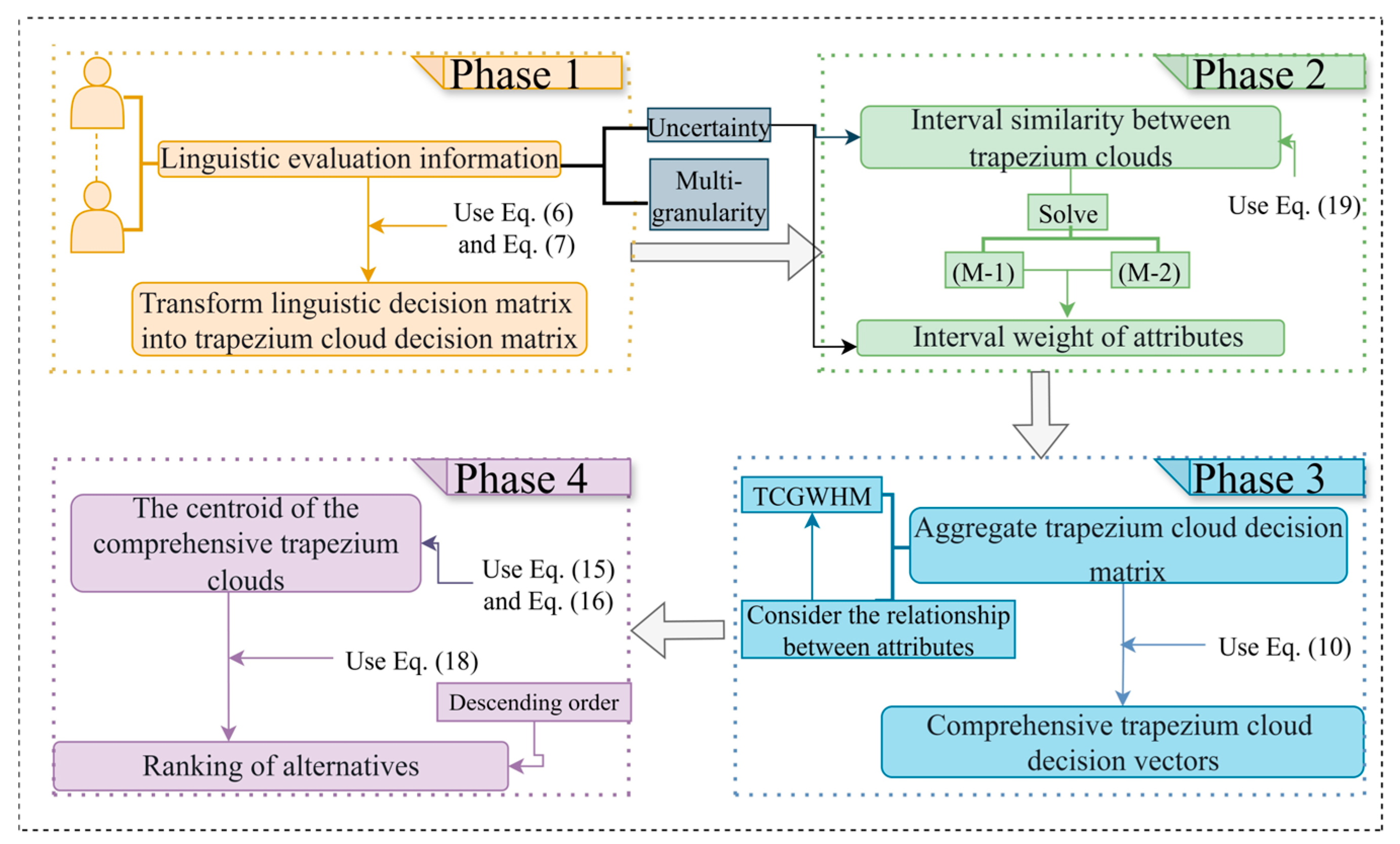
A flowchart is used to demonstrate the trapezium cloud multi-attribute decision-making model proposed in this study, as shown in Figure 7.

7. Numerical Example

In this section, the proposed trapezium cloud multi-attribute decision-making model will be applied to Chinese fir and pine forests in terms of the two dimensions of standing timber quality and standing timber value. Firstly, the standing timber quality of these two types of forest lands will be ranked internally, and then the standing timber value will be accounted for and the corresponding ratings will be completed. In reality, assessing the quality of standing timber using a variety of measuring devices is costly and prone to damage to standing timber. Given the imperfect development of non-destructive measurements, it is reasonable to choose indicators that are easy to observe visually, reflect the quality of standing timber to a greater extent, and can be evaluated directly in linguistic terms. Inspired by Nocetti and Brunetti [54], diameter at breast height, length, straightness, absence of damage, roundness, and crown fullness were chosen as evaluation indicators. Given that evaluation information is more linguistic, probabilistic, and uncertain, it is reasonable for decision-makers to give probabilistic uncertain linguistic terms as decision information. In addition, the linguistic term set provided to the decision-maker for selection is multi granular due to the different knowledge backgrounds of the decision-makers. Therefore, in this study, standing timber quality was evaluated in a probabilistic multi-granularity uncertain linguistic setting. Next, the application of the proposed method is illustrated using some Chinese fir and pine forests as examples.

Let there be 10 forest lands, denoted as $A_1$, $A_2$, $A_3$, $A_4$, $A_5$, $A_6$, $A_7$, $A_8$, $A_9$, and $A_{10}$. Of these, six forest lands of Chinese fir are denoted as $A_1$, $A_2$, $A_3$, $A_4$, $A_5$, and $A_6$, and four forest lands of pine are denoted as $A_7$, $A_8$, $A_9$, and $A_{10}$. Suppose that the decision-maker can autonomously select the preferred linguistic evaluation granularity within the linguistic term set of 3, 5, 7, 9, 11, and 13 granularities. It is assumed that decision-makers evaluate the standing timber quality of Chinese fir and pine forests on the basis of the attributes of diameter at breast height, length, straightness, absence of damage, roundness, and crown fullness, namely, $B_1$, $B_2$, $B_3$, $B_4$, $B_5$, and $B_6$, and obtain the probabilistic multi-granularity uncertain linguistic decision matrices $\overline{\mathrm{{\rm M}}}=\left(\begin{array}{l}{\overline{\mathrm{{\rm M}}}}_1\\ {\overline{\mathrm{{\rm M}}}}_2\end{array}\right)$ for the standing timber quality of Chinese fir forest lands and the standing timber quality of pine forest lands, respectively, where ${\overline{\mathrm{{\rm M}}}}_1$ and ${\overline{\mathrm{{\rm M}}}}_2$ are as follows.

$$\begin{gathered} \begin{array}{cc}{\mathrm{B}}_1 \\ {\overline{\mathrm{{\rm M}}}}_1=\begin{array}{c}{A}_1\hfill \\ A_2\hfill \\ A_3\hfill \\ A_4\hfill \\ A_5\hfill \\ A_6\hfill \end{array}\left(\begin{array}{c}{\{<[\mathrm{s}}_{0_1}^5{,\mathrm{s}}_{1_1}^5],0{.3}_1{>,<[\mathrm{s}}_{1_2}^5{,\mathrm{s}}_{2_2}^5],0{.3}_2{>,<[\mathrm{s}}_{1_3}^7{,\mathrm{s}}_{3_3}^7],0{.4}_3>\} \hfill \\ {\{<[\mathrm{s}}_{2_1}^7{,\mathrm{s}}_{3_1}^7],0{.4}_1{>,<[\mathrm{s}}_{1_2}^5{,\mathrm{s}}_{2_2}^5],0{.6}_2>\} \hfill \\ {\{<[\mathrm{s}}_{{-1}_1}^5{,\mathrm{s}}_{1_1}^5],0{.3}_1{>,<[\mathrm{s}}_{{-2}_2}^7{,\mathrm{s}}_{1_2}^7],0{.4}_2{>,<[\mathrm{s}}_{{-1}_3}^7{,\mathrm{s}}_{0_3}^7],0{.3}_3>\} \hfill \\ {\{<[\mathrm{s}}_{{-1}_1}^3{,\mathrm{s}}_{0_1}^3],0{.4}_1{>,<[\mathrm{s}}_{{-2}_2}^5{,\mathrm{s}}_{{-1}_2}^5],0{.3}_2{>,<[\mathrm{s}}_{{-3}_3}^7{,\mathrm{s}}_{{-2}_3}^7],0{.3}_3>\} \hfill \\ {\{<[\mathrm{s}}_{0_1}^5{,\mathrm{s}}_{1_1}^5],0{.4}_1{>,<[\mathrm{s}}_{0_2}^5{,\mathrm{s}}_{2_2}^5],0{.3}_2{>,<[\mathrm{s}}_{0_3}^7{,\mathrm{s}}_{1_3}^7],0{.2}_3{>,<[\mathrm{s}}_{1_4}^9{,\mathrm{s}}_{2_4}^9],0{.1}_4>\} \hfill \\ {\{<[\mathrm{s}}_{0_1}^5{,\mathrm{s}}_{1_1}^5],0{.4}_1{>,<[\mathrm{s}}_{{-1}_2}^7{,\mathrm{s}}_{1_2}^7],0{.6}_2>\} \hfill \end{array}\right.& { \mathrm{B}}_2 \\ \begin{array}{c}{ \{<[\mathrm{s}}_{0_1}^3{,\mathrm{s}}_{1_1}^3],0{.2}_1{>,<[\mathrm{s}}_{0_2}^5{,\mathrm{s}}_{1_2}^5],0{.5}_2{>,<[\mathrm{s}}_{1_3}^7{,\mathrm{s}}_{2_3}^7],0{.3}_3>\} \hfill \\ {\{<[\mathrm{s}}_{2_1}^7{,\mathrm{s}}_{3_1}^7],0{.2}_1{>,<[\mathrm{s}}_{2_2}^9{,\mathrm{s}}_{3_2}^9],0{.8}_2>\} \hfill \\ { \{<[\mathrm{s}}_{0_1}^3{,\mathrm{s}}_{1_1}^3],0{.4}_1{>,<[\mathrm{s}}_{1_2}^5{,\mathrm{s}}_{1_2}^5],0{.3}_2{>,<[\mathrm{s}}_{{-2}_3}^7{,\mathrm{s}}_{2_3}^7],0{.3}_3>\} \hfill \\ {\{<[\mathrm{s}}_{-1_1}^5{,\mathrm{s}}_{1_1}^5],0{.7}_1{>,<[\mathrm{s}}_{-2_2}^7{,\mathrm{s}}_{1_2}^7],0{.3}_2>\} \hfill \\ {\{<[\mathrm{s}}_{-2_1}^7{,\mathrm{s}}_{1_1}^7],0{.1}_1{>,<[\mathrm{s}}_{-2_2}^7{,\mathrm{s}}_{-1_2}^7],0{.5}_2{>,<[\mathrm{s}}_{{-1}_3}^9{,\mathrm{s}}_{0_3}^9],0{.4}_3>\} \hfill \\ {\{<[\mathrm{s}}_{-1_1}^3{,\mathrm{s}}_{0_1}^3],0{.3}_1{>,<[\mathrm{s}}_{0_2}^5{,\mathrm{s}}_{1_2}^5],0{.5}_2{>,<[\mathrm{s}}_{{-1}_3}^7{,\mathrm{s}}_{1_3}^7],0{.2}_3>\} \hfill \end{array}\\ {\mathrm{B}}_3 \\ \begin{array}{c}{\{<[\mathrm{s}}_{{-1}_1}^5{,\mathrm{s}}_{1_1}^5],0{.4}_1{>,<[\mathrm{s}}_{0_2}^7{,\mathrm{s}}_{1_2}^7],0{.6}_2>\} \hfill \\ {\{<[\mathrm{s}}_{1_1}^7{,\mathrm{s}}_{3_1}^5],0{.4}_1{>,<[\mathrm{s}}_{2_2}^7{,\mathrm{s}}_{3_2}^7],0{.4}_2{>,<[\mathrm{s}}_{2_3}^9{,\mathrm{s}}_{4_3}^9],0{.2}_3>\} \hfill \\ {\{<[\mathrm{s}}_{{-2}_1}^5{,\mathrm{s}}_{0_1}^5],0{.2}_1{>,<[\mathrm{s}}_{{-1}_2}^7{,\mathrm{s}}_{0_2}^7],0{.8}_2>\} \hfill \\ {\{<[\mathrm{s}}_{{-2}_1}^5{,\mathrm{s}}_{0_1}^5],0{.3}_1{>,<[\mathrm{s}}_{{-1}_2}^7{,\mathrm{s}}_{1_2}^7],0{.3}_2{>,<[\mathrm{s}}_{{-2}_3}^7{,\mathrm{s}}_{{-1}_3}^7],0{.3}_3{>,<[\mathrm{s}}_{{-2}_4}^9{,\mathrm{s}}_{{-1}_4}^9],0{.1}_4>\} \hfill \\ {\{<[\mathrm{s}}_{{-2}_1}^5{,\mathrm{s}}_{0_1}^5],0{.8}_1{>,<[\mathrm{s}}_{{-1}_2}^7{,\mathrm{s}}_{1_2}^7],0{.2}_2>\} \hfill \\ {\{<[\mathrm{s}}_{{-1}_1}^5{,\mathrm{s}}_{0_1}^5],0{.2}_1{>,<[\mathrm{s}}_{{-2}_2}^7{,\mathrm{s}}_{1_2}^7],0{.3}_2{>,<[\mathrm{s}}_{{-1}_3}^7{,\mathrm{s}}_{0_3}^7],0{.2}_3{>,<[\mathrm{s}}_{{-2}_4}^9{,\mathrm{s}}_{0_4}^9],0{.3}_4>\} \hfill \end{array}& { \mathrm{B}}_4 \\ \begin{array}{c}{\{<[\mathrm{s}}_{1_1}^5{,\mathrm{s}}_{2_1}^5],0{.2}_1{>,<[\mathrm{s}}_{{-1}_2}^7{,\mathrm{s}}_{2_2}^7],0{.2}_2{>,<[\mathrm{s}}_{0_3}^7{,\mathrm{s}}_{1_3}^7],0{.3}_3{>,<[\mathrm{s}}_{{-1}_4}^9{,\mathrm{s}}_{2_4}^9],0{.3}_4>\} \hfill \\ {\{<[\mathrm{s}}_{0_1}^3{,\mathrm{s}}_{1_1}^3],0{.6}_1{>,<[\mathrm{s}}_{{-1}_2}^5{,\mathrm{s}}_{2_2}^5],0{.2}_2{>,<[\mathrm{s}}_{1_3}^5{,\mathrm{s}}_{2_3}^5],0{.2}_3>\} \hfill \\ {\{<[\mathrm{s}}_{0_1}^3{,\mathrm{s}}_{1_1}^3],0{.4}_1{>,<[\mathrm{s}}_{{-2}_2}^5{,\mathrm{s}}_{2_2}^5],0{.4}_2{>,<[\mathrm{s}}_{-1_3}^7{,\mathrm{s}}_{0_3}^7],0{.2}_3>\} \hfill \\ {\{<[\mathrm{s}}_{0_1}^3{,\mathrm{s}}_{0_1}^3],0{.6}_1{>,<[\mathrm{s}}_{0_2}^5{,\mathrm{s}}_{0_2}^5],0{.4}_2>\} \hfill \\ {\{<[\mathrm{s}}_{-2_1}^7{,\mathrm{s}}_{1_1}^7],0{.3}_1{>,<[\mathrm{s}}_{{-1}_2}^7{,\mathrm{s}}_{2_2}^7],0{.3}_2{>,<[\mathrm{s}}_{-2_3}^9{,\mathrm{s}}_{0_3}^9],0{.2}_3{>,<[\mathrm{s}}_{{-1}_4}^9{,\mathrm{s}}_{1_4}^9],0{.2}_4>\}\hfill \\ {\{<[\mathrm{s}}_{0_1}^7{,\mathrm{s}}_{1_1}^7],0{.4}_1{>,<[\mathrm{s}}_{{-2}_2}^7{,\mathrm{s}}_{2_2}^7],0{.2}_2{>,<[\mathrm{s}}_{-1_3}^9{,\mathrm{s}}_{2_3}^9],0{.4}_3>\} \hfill \end{array}\\ {\mathrm{B}}_5 \\ \begin{array}{c}{\{<[\mathrm{s}}_{-1_1}^5{,\mathrm{s}}_{2_1}^5],0{.2}_1{>,<[\mathrm{s}}_{0_2}^5{,\mathrm{s}}_{1_2}^5],0{.4}_2{>,<[\mathrm{s}}_{1_3}^7{,\mathrm{s}}_{2_3}^7],0{.3}_3{>,<[\mathrm{s}}_{1_4}^9{,\mathrm{s}}_{3_4}^9],0{.1}_4>\}\hfill \\ {\{<[\mathrm{s}}_{2_1}^7{,\mathrm{s}}_{3_1}^7],0{.8}_1{>,<[\mathrm{s}}_{3_2}^9{,\mathrm{s}}_{4_2}^9],0{.2}_2>\} \hfill \\ {\{<[\mathrm{s}}_{-1_1}^5{,\mathrm{s}}_{0_1}^5],0{.6}_1{>,<[\mathrm{s}}_{-1_2}^7{,\mathrm{s}}_{1_2}^7],0{.4}_2>\} \hfill \\ {\{<[\mathrm{s}}_{-2_1}^5{,\mathrm{s}}_{-1_1}^5],0{.2}_1{>,<[\mathrm{s}}_{-1_2}^5{,\mathrm{s}}_{0_2}^5],0{.7}_2{>,<[\mathrm{s}}_{-2_3}^7{,\mathrm{s}}_{1_3}^7],0{.1}_3>\} \hfill \\ {\{<[\mathrm{s}}_{0_1}^5{,\mathrm{s}}_{1_1}^5],0{.4}_1{>,<[\mathrm{s}}_{0_2}^7{,\mathrm{s}}_{1_2}^7],0{.6}_2>\} \hfill \\ {\{<[\mathrm{s}}_{-1_1}^5{,\mathrm{s}}_{2_1}^5],0{.2}_1{>,<[\mathrm{s}}_{0_2}^5{,\mathrm{s}}_{1_2}^5],0{.4}_2{>,<[\mathrm{s}}_{-2_3}^7{,\mathrm{s}}_{2_3}^7],0{.3}_3>\} \hfill \end{array}& { \mathrm{B}}_6 \\ \left.\begin{array}{c}{\{<[\mathrm{s}}_{0_1}^3{,\mathrm{s}}_{1_1}^3],0{.6}_1{>,<[\mathrm{s}}_{1_2}^5{,\mathrm{s}}_{2_2}^5],0{.4}_2>\} \hfill \\ { \{<[\mathrm{s}}_{0_1}^3{,\mathrm{s}}_{1_1}^3],0{.4}_1{>,<[\mathrm{s}}_{1_2}^5{,\mathrm{s}}_{2_2}^5],0{.2}_2{>,<[\mathrm{s}}_{1_3}^7{,\mathrm{s}}_{3_3}^7],0{.2}_3{>,<[\mathrm{s}}_{2_4}^7{,\mathrm{s}}_{3_4}^7],0{.2}_4>\} \hfill \\ { \{<[\mathrm{s}}_{-1_1}^3{,\mathrm{s}}_{0_1}^3],0{.3}_1{>,<[\mathrm{s}}_{0_2}^5{,\mathrm{s}}_{1_2}^5],0{.1}_2{>,<[\mathrm{s}}_{-1_3}^5{,\mathrm{s}}_{1_3}^5],0{.4}_3{>,<[\mathrm{s}}_{-1_4}^7{,\mathrm{s}}_{1_4}^7],0{.2}_4>\} \hfill \\ {\{<[\mathrm{s}}_{-2_1}^5{,\mathrm{s}}_{-1_1}^5],0{.7}_1{>,<[\mathrm{s}}_{-2_2}^7{,\mathrm{s}}_{0_2}^7],0{.3}_2>\} \hfill \\ {\{<[\mathrm{s}}_{-1_1}^5{,\mathrm{s}}_{1_1}^5],0{.3}_1{>,<[\mathrm{s}}_{-2_2}^5{,\mathrm{s}}_{1_2}^5],0{.4}_2{>,<[\mathrm{s}}_{-1_3}^7{,\mathrm{s}}_{2_3}^7],0{.3}_3>\} \hfill \\ {\{<[\mathrm{s}}_{-2_1}^7{,\mathrm{s}}_{0_1}^7],0{.6}_1{>,<[\mathrm{s}}_{-1_2}^9{,\mathrm{s}}_{1_2}^9],0{.4}_2>\} \hfill \end{array}\right)\end{array} \end{gathered}$$

$$\begin{gathered} \begin{array}{cc}{\mathrm{B}}_1 \\ {\overline{\mathrm{{\rm M}}}}_2=\begin{array}{c}{A}_7\hfill \\ A_8\hfill \\ A_9\hfill \\ A_{10}\hfill \end{array}\left(\begin{array}{c}{\{<[\mathrm{s}}_{0_1}^3{,\mathrm{s}}_{1_1}^3],0{.4}_1{>,<[\mathrm{s}}_{-1_2}^5{,\mathrm{s}}_{2_2}^5],0{.2}_2{>,<[\mathrm{s}}_{0_3}^5{,\mathrm{s}}_{1_3}^5],0{.2}_3{>,<[\mathrm{s}}_{1_4}^7{,\mathrm{s}}_{2_4}^7],0{.2}_4>\} \hfill \\ {\{<[\mathrm{s}}_{-1_1}^5{,\mathrm{s}}_{0_1}^5],0{.2}_1{>,<[\mathrm{s}}_{0_2}^5{,\mathrm{s}}_{1_2}^5],0{.4}_2{>,<[\mathrm{s}}_{-1_3}^7{,\mathrm{s}}_{0_3}^7],0{.3}_3{>,<[\mathrm{s}}_{0_4}^7{,\mathrm{s}}_{1_4}^7],0{.1}_4>\}\hfill \\ {\{<[\mathrm{s}}_{1_1}^5{,\mathrm{s}}_{2_1}^5],0{.4}_1{>,<[\mathrm{s}}_{1_2}^7{,\mathrm{s}}_{3_2}^7],0{.2}_2{>,<[\mathrm{s}}_{2_3}^7{,\mathrm{s}}_{3_3}^7],0{.1}_3{>,<[\mathrm{s}}_{2_4}^9{,\mathrm{s}}_{3_4}^9],0{.3}_4>\} \hfill \\ {\{<[\mathrm{s}}_{-1_1}^3{,\mathrm{s}}_{0_1}^3],0{.2}_1{>,<[\mathrm{s}}_{-2_2}^5{,\mathrm{s}}_{-1_2}^5],0{.3}_2{>,<[\mathrm{s}}_{-2_3}^7{,\mathrm{s}}_{0_3}^7],0{.5}_3>\} \hfill \end{array}\right.& { \mathrm{B}}_2 \\ \begin{array}{c}{\{<[\mathrm{s}}_{-1_1}^5{,\mathrm{s}}_{1_1}^5],0{.4}_1{>,<[\mathrm{s}}_{0_2}^5{,\mathrm{s}}_{1_2}^5],0{.5}_2{>,<[\mathrm{s}}_{-1_3}^7{,\mathrm{s}}_{2_3}^7],0{.3}_3>\} \hfill \\ {\{<[\mathrm{s}}_{0_1}^5{,\mathrm{s}}_{1_1}^5],0{.4}_1{>,<[\mathrm{s}}_{0_2}^7{,\mathrm{s}}_{0_2}^7],0{.3}_2{>,<[\mathrm{s}}_{1_3}^7{,\mathrm{s}}_{2_3}^7],0{.3}_3>\} \hfill \\ { \{<[\mathrm{s}}_{0_1}^5{,\mathrm{s}}_{1_1}^5],0{.2}_1{>,<[\mathrm{s}}_{1_2}^7{,\mathrm{s}}_{2_2}^7],0{.4}_2{>,<[\mathrm{s}}_{1_3}^7{,\mathrm{s}}_{3_3}^7],0{.1}_3{>,<[\mathrm{s}}_{0_4}^9{,\mathrm{s}}_{2_4}^9],0{.3}_4>\}\hfill \\ {\{<[\mathrm{s}}_{-2_1}^7{,\mathrm{s}}_{-1_1}^7],0{.4}_1{>,<[\mathrm{s}}_{-2_2}^7{,\mathrm{s}}_{0_2}^7],0{.2}_2{>,<[\mathrm{s}}_{-3_3}^9{,\mathrm{s}}_{-1_3}^9],0{.4}_3>\} \hfill \end{array}\\ {\mathrm{B}}_3 \\ \begin{array}{c}{\{<[\mathrm{s}}_{1_1}^5{,\mathrm{s}}_{2_1}^5],0{.8}_1{>,<[\mathrm{s}}_{0_2}^7{,\mathrm{s}}_{1_2}^7],0{.2}_2>\} \hfill \\ {\{<[\mathrm{s}}_{-1_1}^7{,\mathrm{s}}_{1_1}^7],0{.2}_1{>,<[\mathrm{s}}_{0_2}^7{,\mathrm{s}}_{2_2}^7],0{.6}_2{>,<[\mathrm{s}}_{-1_3}^9{,\mathrm{s}}_{1_3}^9],0{.2}_3>\}\hfill \\ {\{<[\mathrm{s}}_{1_1}^7{,\mathrm{s}}_{3_1}^7],0{.7}_1{>,<[\mathrm{s}}_{1_2}^9{,\mathrm{s}}_{3_2}^9],0{.3}_2>\} \hfill \\ {\{<[\mathrm{s}}_{-1_1}^5{,\mathrm{s}}_{0_1}^5],0{.5}_1{>,<[\mathrm{s}}_{-1_2}^7{,\mathrm{s}}_{1_2}^7],0{.5}_2>\} \hfill \end{array}& {\mathrm{B}}_4 \\ \begin{array}{c}{ \{<[\mathrm{s}}_{0_1}^5{,\mathrm{s}}_{1_1}^5],0{.2}_1{>,<[\mathrm{s}}_{1_2}^5{,\mathrm{s}}_{2_2}^5],0{.3}_2{>,<[\mathrm{s}}_{-1_3}^7{,\mathrm{s}}_{2_3}^7],0{.4}_3{>,<[\mathrm{s}}_{0_4}^9{,\mathrm{s}}_{1_4}^9],0{.1}_4>\} \hfill \\ {\{<[\mathrm{s}}_{0_1}^7{,\mathrm{s}}_{2_1}^7],0{.8}_1{>,<[\mathrm{s}}_{0_2}^9{,\mathrm{s}}_{1_2}^9],0{.2}_2>\} \hfill \\ {\{<[\mathrm{s}}_{2_1}^7{,\mathrm{s}}_{3_1}^7],0{.5}_1{>,<[\mathrm{s}}_{0_2}^9{,\mathrm{s}}_{2_2}^9],0{.4}_2{>,<[\mathrm{s}}_{1_3}^9{,\mathrm{s}}_{3_3}^9],0{.1}_3>\} \hfill \\ { \{<[\mathrm{s}}_{-2_1}^5{,\mathrm{s}}_{0_1}^5],0{.3}_1{>,<[\mathrm{s}}_{-1_2}^5{,\mathrm{s}}_{1_2}^5],0{.3}_2{>,<[\mathrm{s}}_{-2_3}^7{,\mathrm{s}}_{1_3}^7],0{.3}_3{>,<[\mathrm{s}}_{-1_4}^9{,\mathrm{s}}_{0_4}^9],0{.1}_4>\}\hfill \end{array}\\ { \mathrm{B}}_5 \\ \begin{array}{c}{\{<[\mathrm{s}}_{0_1}^3{,\mathrm{s}}_{1_1}^3],0{.1}_1{>,<[\mathrm{s}}_{0_2}^5{,\mathrm{s}}_{2_2}^5],0{.2}_2{>,<[\mathrm{s}}_{1_3}^7{,\mathrm{s}}_{1_3}^7],0{.3}_3{>,<[\mathrm{s}}_{1_4}^7{,\mathrm{s}}_{2_4}^7],0{.4}_4>\}\hfill \\ {\{<[\mathrm{s}}_{0_1}^3{,\mathrm{s}}_{1_1}^3],0{.5}_1{>,<[\mathrm{s}}_{1_2}^5{,\mathrm{s}}_{2_2}^5],0{.2}_2{>,<[\mathrm{s}}_{-1_3}^7{,\mathrm{s}}_{1_3}^7],0{.3}_3>\} \hfill \\ {\{<[\mathrm{s}}_{1_1}^5{,\mathrm{s}}_{1_1}^5],0{.3}_1{>,<[\mathrm{s}}_{1_2}^7{,\mathrm{s}}_{2_2}^7],0{.3}_2{>,<[\mathrm{s}}_{2_3}^9{,\mathrm{s}}_{4_3}^9],0{.4}_3>\} \hfill \\ {\{<[\mathrm{s}}_{0_1}^5{,\mathrm{s}}_{0_1}^5],0{.1}_1{>,<[\mathrm{s}}_{-1_2}^5{,\mathrm{s}}_{1_2}^5],0{.7}_2{>,<[\mathrm{s}}_{0_3}^7{,\mathrm{s}}_{1_3}^7],0{.2}_3>\} \hfill \end{array}& { \mathrm{B}}_6 \\ \left.\begin{array}{c}{\{<[\mathrm{s}}_{1_1}^5{,\mathrm{s}}_{1_1}^5],0{.5}_1{>,<[\mathrm{s}}_{-1_2}^7{,\mathrm{s}}_{2_2}^7],0{.5}_2>\} \hfill \\ {\{<[\mathrm{s}}_{-1_1}^5{,\mathrm{s}}_{1_1}^5],0{.7}_1{>,<[\mathrm{s}}_{-2_2}^9{,\mathrm{s}}_{0_2}^9],0{.3}_2>\} \hfill \\ { \{<[\mathrm{s}}_{0_1}^3{,\mathrm{s}}_{1_1}^3],0{.1}_1{>,<[\mathrm{s}}_{-1_2}^5{,\mathrm{s}}_{2_2}^5],0{.4}_2{>,<[\mathrm{s}}_{0_3}^7{,\mathrm{s}}_{3_3}^7],0{.5}_3>\}\hfill \\ {\{<[\mathrm{s}}_{-2_1}^7{,\mathrm{s}}_{1_1}^7],0{.6}_1{>,<[\mathrm{s}}_{-1_2}^9{,\mathrm{s}}_{0_2}^9],0{.4}_2>\} \hfill \end{array}\right)\end{array} \end{gathered}$$

Let the discourse domain $U=[0,10]$. The probabilistic multi-granularity uncertain linguistic decision matrix $\overline{\mathrm{{\rm M}}}$ is transformed into a trapezium cloud decision matrix $\widetilde{\mathrm{{\rm M}}}=\left(\begin{array}{l}{\widetilde{\mathrm{{\rm M}}}}_1\\ {\widetilde{\mathrm{{\rm M}}}}_2\end{array}\right)$, where ${\widetilde{\mathrm{{\rm M}}}}_1$ and ${\widetilde{\mathrm{{\rm M}}}}_2$ are as follows, respectively.

$$\begin{gathered} \begin{array}{ccc}{ \mathrm{B}}_1 \\ {\widetilde{\mathrm{{\rm M}}}}_1=\begin{array}{c}{A}_1\\ A_2\\ A_3\\ A_4\\ A_5\\ A_6\end{array}\left(\begin{array}{c}([6.82,9.52],0.64,0.08)\\ ([8.80,10.00],0.47,0.07)\\ ([1.62,6.82],0.89,0.11)\\ ([0.00,2.66],0.66,0.09)\\ ([5.12,8.60],0.78,0.11)\\ ([3.80,7.56],1.12,0.11)\end{array}\right.& { \mathrm{B}}_2 \\ \begin{array}{c}([5.60,9.02],0.77,0.12)\\ ([8.60,9.76],0.36,0.04)\\ ([4.70,9.34],0.87,0.15)\\ ([1.30,7.98],0.98,0.14)\\ ([1.88,7.40],0.88,0.11)\\ ([3.10,7.10],0.84,0.11)\end{array}& { \mathrm{B}}_3 \\ \begin{array}{c}([3.64,7.56],0.81,0.11)\\ ([8.24,10.00],0.44,0.05)\\ ([2.40,5.00],0.71,0.09)\\ ([1.24,4.88],0.74,0.10)\\ ([0.60,5.40],0.87,0.12)\\ ([1.58,5.60],0.79,0.10)\end{array}\\ { \mathrm{B}}_4 \\ \begin{array}{c}([4.92,8.50],0.76,0.09)\\ ([5.00,10.00],0.90,0.17)\\ ([2.60,9.00],0.96,0.16)\\ ([5.00,8.00],0.82,0.16)\\ ([2.16,7.16],0.86,0.11)\\ ([3.64,8.04],0.82,0.09)\end{array}& { \mathrm{B}}_5 \\ \begin{array}{c}([5.04,9.15],0.77,0.11)\\ ([9.46,10.00],0.30,0.04)\\ ([2.16,5.80],0.82,0.11)\\ ([1.18,4.52],0.78,0.11)\\ ([5.00,7.56],0.72,0.09)\\ ([2.50,8.18],0.91,0.13)\end{array}& { \mathrm{B}}_6 \\ \left.\begin{array}{c}([6.36,10.00],0.80,0.16)\\ ([6.96,10.00],0.70,0.13)\\ ([2.34,8.50],1.00,0.15)\\ ([0.18,2.62],0.63,0.09)\\ ([1.38,8.70],1.00,0.14)\\ ([1.88,5.48],0.74,0.08)\end{array}\right)\end{array} \end{gathered}$$

$$\begin{gathered} \begin{array}{ccc}{ \mathrm{B}}_1 \\ {\widetilde{\mathrm{{\rm M}}}}_2=\begin{array}{c}{A}_7\\ A_8\\ A_9\\ A_{10}\end{array}\left(\begin{array}{c}([4.72,9.56],0.84,0.12)\\ ([3.72,6.56],0.75,0.10)\\ ([7.38,8.91],0.46,0.06)\\ ([0.30,3.98],0.73,0.09)\end{array}\right.& { \mathrm{B}}_2 \\ \begin{array}{c}([3.72,8.70],0.89,0.12)\\ ([5.60,7.68],0.64,0.09)\\ ([6.00,8.96],0.64,0.08)\\ ([0.48,3.72],0.59,0.07)\end{array}& { \mathrm{B}}_3 \\ \begin{array}{c}([7.72,9.40],0.58,0.08)\\ ([4.36,8.28],0.77,0.09)\\ ([6.76,9.91],0.56,0.07)\\ ([2.70,6.00],0.82,0.11)\end{array}\\ {\mathrm{B}}_4 \\ \begin{array}{c}([5.22,9.06],0.79,0.10)\\ ([5.00,9.24],0.81,0.11)\\ ([7.32,9.33],0.51,0.06)\\ ([0.96,6.62],0.92,0.13)\end{array}& { \mathrm{B}}_5 \\ \begin{array}{c}([6.40,8.86],0.64,0.09)\\ ([5.08,9.10],0.81,0.10)\\ ([7.98,9.34],0.47,0.07)\\ ([2.62,7.78],0.90,0.13)\end{array}& { \mathrm{B}}_6 \\ \left.\begin{array}{c}([5.70,8.90],0.76,0.09)\\ ([1.60,7.38],0.90,0.13)\\ ([3.64,10.00],0.91,0.12)\\ ([1.88,3.80],0.52,0.06)\end{array}\right)\end{array} \end{gathered}$$

The interval similarities $si{m}_{[{\widehat{C}}_{ij},{\widehat{C}}_{kj}]},i=1,\dots ,6;k=i+1,\dots ,6;j=1,\dots ,6$ and $si{m}_{[{\widehat{C}}_{ij},{\widehat{C}}_{kj}]},i=7,\dots ,10; k=i+1,\dots ,10; j=1,\dots ,6$ between the trapezium clouds in ${\widetilde{\mathrm{{\rm M}}}}_1$ and ${\widetilde{\mathrm{{\rm M}}}}_2$ are measured using Equation (19). Based on this, the optimization models (M-1) and (M-2) are solved to obtain the normalized interval weights ${\tilde{\omega }}_j=[{\omega }_j^{-},{\omega }_j^{+}], j=1,\dots ,6$ of the attributes in ${\widetilde{\mathrm{{\rm M}}}}_1$ and ${\widetilde{\mathrm{{\rm M}}}}_2$, respectively, as shown in

Table 2. Normalized interval weights of Chinese fir and pine.

	${\mathit{B}}_1$	${\mathit{B}}_2$	${\mathit{B}}_3$	${\mathit{B}}_4$	${\mathit{B}}_5$	${\mathit{B}}_6$
Chinese fir	[0.04, 0.12]	[0.05, 0.19]	[0.04, 0.19]	[0.03, 0.18]	[0.07, 0.21]	[0.06, 0.21]
Pine	[0.10, 0.19]	[0.09, 0.18]	[0.09.0.18]	[0.09, 0.18]	[0.08, 0.17]	[0.10, 0.19]

.

Trapezium clouds are aggregated using Equation (10), and assuming $p=q=1$, the integrated trapezium cloud vector $V=\left(\begin{array}{l}{v}_1\\ v_2\end{array}\right)$ is obtained, where ${\nu }_1$ and ${\nu }_2$ are as follows.

$${\nu }_1=\left(\begin{array}{l}([5.3533,8.9788],0.7672,0.1158)\\ ([7.8913,9.9589],0.5276,0.0844)\\ ([2.7031,7.4282],0.8753,0.1293)\\ ([1.5626,5.1768],0.7719,0.1152)\\ ([2.6768,7.4626],0.8566,0.1138)\\ ([2.6541,6.9505],0.8544,0.1037)\end{array}\right),{\nu }_2=\left(\begin{array}{l}([5.5768,9.0844],0.7540,0.1004)\\ ([4.1937,8.0074],0.7823,0.1040)\\ ([6.4786,9.4143],0.6006,0.0778)\\ ([1.5144,5.2789],0.7428,0.0977)\end{array}\right)$$

Taking the six trapezium clouds corresponding to the first alternative in the first decision matrix as an example, the three-dimensional simulation of the generalized weighted Heronian mean of the trapezium clouds is plotted, as shown in Figure 8.

The approximate centroid $\eta ({\widehat{C}}_i)=(x_{{\widehat{C}}_i},y_{{\widehat{C}}_i}),i=1,\dots ,10$ of the integrated trapezium cloud is calculated using Equations (15) and (16) and is shown in

Table 3. The approximate centroid of integrated trapezium clouds ${\widehat{C}}_i, i=1,\dots ,10$.

$$\mathit{\eta }({\widehat{\mathit{C}}}_1)$$	$$\mathit{\eta }({\widehat{\mathit{C}}}_2)$$	$$\mathit{\eta }({\widehat{\mathit{C}}}_3)$$	$$\mathit{\eta }({\widehat{\mathit{C}}}_4)$$	$$\mathit{\eta }({\widehat{\mathit{C}}}_5)$$	$$\mathit{\eta }({\widehat{\mathit{C}}}_6)$$	$$\mathit{\eta }({\widehat{\mathit{C}}}_7)$$	$$\mathit{\eta }({\widehat{\mathit{C}}}_8)$$	$$\mathit{\eta }({\widehat{\mathit{C}}}_9)$$	$$\mathit{\eta }({\widehat{\mathit{C}}}_{10})$$
(7.1661, 0.1142)	(8.9251, 0.1134)	(5.0657, 0.1132)	(3.3697, 0.1143)	(5.0697, 0.1155)	(4.8023, 0.1163)	(7.3306, 0.1155)	(6.1006, 0.1155)	(7.9465, 0.1158)	(3.3967, 0.1156)

.

Using Equation (18), $T_i,i\in \{1,2,3,\dots 10\}$ is calculated as shown in

Table 4. The values of $T_i$.

${\mathit{T}}_1$	${\mathit{T}}_2$	${\mathit{T}}_3$	${\mathit{T}}_4$	${\mathit{T}}_5$	${\mathit{T}}_6$	${\mathit{T}}_7$	${\mathit{T}}_8$	${\mathit{T}}_9$	${\mathit{T}}_{10}$
0.8180	1.0123	0.5734	0.3851	0.5855	0.5583	0.8465	0.7046	0.9198	0.3926

.

In view of this, the integrated trapezium cloud was ranked, and the ranking relationships were obtained as $A_2\succ A_1\succ A_5\succ A_3\succ A_6\succ A_4$ and $A_9\succ A_7\succ A_8\succ A_{10}$. As a result, by applying the trapezium cloud multi-attribute decision-making model proposed in this study, the ranking of standing timber quality of six Chinese fir forest lands and four pine forest lands was realized.

There are many practical reasons for accounting for standing timber value. For example, in terms of economic development, accounting for standing timber value helps assess the economic value of forests, an important part of national economic development. In terms of ecological protection, accounting for standing timber value enables relevant forestry departments to develop policies that promote sustainable ecological development. Therefore, the accounting of standing timber value has received the attention of many scholars and is a hot area of research, and many scholars have proposed different formulas for accounting standing timber value. Among them, Xu et al. [55] related the accounting of standing timber value to yield rate, and it is obvious that under ideal conditions, the higher the quality of standing timber, the higher the yield rate of the forest land. This study expects to establish a link between standing timber quality and standing timber value. In view of this, the method of Xu et al. was further improved to correlate yield rate with the integrated trapezium cloud, whereby the standing timber values corresponding to the 10 forest lands were accounted for and rated.

Let the integrated trapezium cloud of standing timber quality of the forest land be ${\widehat{C}}_i=([{\underset{¯}{Ex}}_{(i)},{\overline{Ex}}_{(i)}],E{n}_{(i)},H{e}_{(i)})$ and the discourse domain $U=[X_{\min },X_{\max }]$. Then, the formula for the yield rate of the forest land is as follows:

$$K_i={({({\displaystyle \frac{\frac{1}{2}({\underset{¯}{Ex}}_{(i)}+{\overline{Ex}}_{(i)})-X_{\min }}{X_{\max }-X_{\min }}})}^{\ln (e+E{n}_{(i)})})}^{\ln (e+H{e}_{(i)})}$$

(20)

Using Equation (20), the yield rate of the 10 forest lands was calculated as shown in

Table 5. Yield rates of $A_i, i\in \{1,2,3,\dots ,10\}$.

${\mathit{K}}_1$	${\mathit{K}}_2$	${\mathit{K}}_3$	${\mathit{K}}_4$	${\mathit{K}}_5$	${\mathit{K}}_6$	${\mathit{K}}_7$	${\mathit{K}}_8$	${\mathit{K}}_9$	${\mathit{K}}_{10}$
0.6483	0.8711	0.4024	0.2427	0.4062	0.3795	0.6699	0.5260	0.7531	0.2496

.

Further, the formula for accounting for the standing timber value of forest lands through the integrated trapezium cloud ${\widehat{C}}_i=([{\underset{¯}{Ex}}_{(i)},{\overline{Ex}}_{(i)}],E{n}_{(i)},H{e}_{(i)})$ of forest land standing timber quality is as follows:

$$B_i=M{({({\displaystyle \frac{\frac{1}{2}({\underset{¯}{Ex}}_{(i)}+{\overline{Ex}}_{(i)})-X_{\min }}{X_{\max }-X_{\min }}})}^{\ln (e+E{n}_{(i)})})}^{\ln (e+H{e}_{(i)})}A$$

(21)

where $M$ is the stock volume, and $A$ is the net profit per unit.

Suppose the stock volume of Chinese fir forest is 2,500,000 m³, and the net profit per unit is 500 CNY/m³. Furthermore, the stock volume of pine forest is 1,000,000 m³, and the net profit per unit is 240 CNY/m³. The standing timber value of the 10 forest lands is obtained according to Equation (21), as shown in

Table 6. Standing timber values of $A_i, i\in \{1,2,3,\dots ,10\}$.

${\mathit{B}}_1$	${\mathit{B}}_2$	${\mathit{B}}_3$	${\mathit{B}}_4$	${\mathit{B}}_5$	${\mathit{B}}_6$	${\mathit{B}}_7$	${\mathit{B}}_8$	${\mathit{B}}_9$	${\mathit{B}}_{10}$
810.375	1088.875	503.000	303.375	507.750	474.375	160.776	126.240	180.744	59.904

(unit is in million CNY).

Therefore, the ranking of the standing timber value of the 10 forest lands is $A_2>A_1>A_5>A_3>A_6>A_4>A_9>A_7>A_8>A_{10}$. According to the difference in standing timber value, these 10 forest lands are categorized into five levels, as shown in

Table 7. Five levels of $A_i, i\in \{1,2,\dots ,10\}$.

Levels	Standing Timber Values	Forest Lands
I	$>750$	$A_1$$, A_2$
II	$>500$ and $\le 750$	$A_3$$, A_5$
III	$>250$ and $\le 500$	$A_4$$, A_6$
IV	$>100$ and $\le 250$	$A_7$$, A_8$$, A_9$
V	$\le 100$	$A_{10}$

and Figure 9.

The core conclusions of this method can directly provide three types of practical support for forestry departments. First, prioritization of resource management and protection: Based on the quality ranking results (e.g., Chinese fir forest land $A_2$ and pine forest land $A_9$ have the best quality, while $A_4$ and $A_{10}$ have poor quality), departments can allocate limited management and protection resources to low-quality forest lands. For $A_4$, which has problems of small diameter at breast height and poor straightness, targeted tending measures (such as thinning and trunk correction) can be carried out; for high-quality forest lands like $A_2$, only regular monitoring is needed to maximize the efficiency of management and protection. Second, support for development and utilization decision-making: The value accounting results can assist in formulating logging quotas and ecological compensation standards. For high-value forest lands (such as $A_2$), “limited and sustainable logging” can be adopted, and the logging volume can be controlled according to the yield rate (0.8711) derived from the trapezium cloud to balance economic benefits and ecological protection. Third, simplification of the evaluation process: Instead of relying on expensive measurement instruments, departments can only train front-line staff to collect probabilistic multi-granularity uncertain linguistic information and then substitute this information into the method to complete the evaluation. This greatly reduces the cost of large-scale forest land surveys and the damage to trees and is especially suitable for remote forest lands where instrument measurement is difficult to carry out.

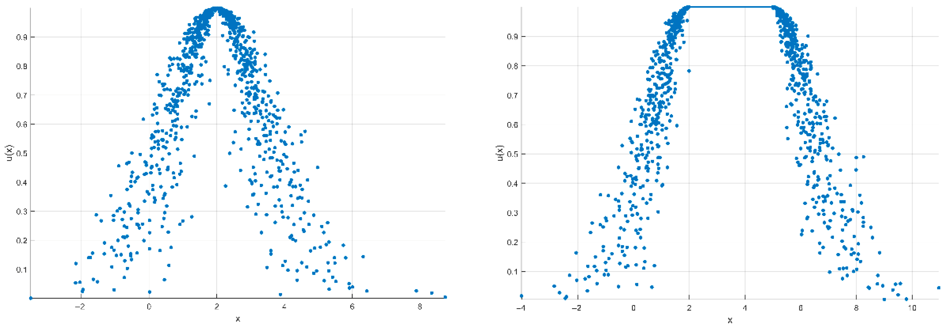
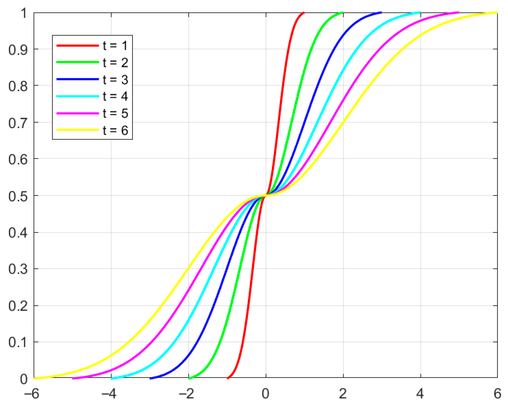
8. Comparison Analysis

This section carries out a comparison analysis to compare the proposed multi-attribute decision-making model with some existing multi-attribute decision-making models in multiple dimensions. This section also designs a comparison numerical example to jointly get the ranking between the proposed trapezium cloud ranking method in this study and some existing trapezium cloud ranking methods through three cases in order to demonstrate the rationality and superiority of the proposed trapezium clouds ranking methods.

In order to demonstrate the rationality and superiority of the trapezium cloud multi-attribute decision-making model in the probabilistic multi-granularity uncertain linguistic setting proposed in this study, it is compared with some other multi-attribute decision-making models in some other linguistic settings in several dimensions, as shown in

Table 8. Comparison results with other multi-attribute decision-making models.

	References	Linguistic Assessment Information	Information Processing Method	Multi-Granularity Linguistic	Relationships between Attributes	Uncertainty
Improved approach based on deviation and TOPSIS	Liu et al. [56]	MGLTSs	Subscripts operation	√	╳	╳
Possibility degree matrix-based approach	Wang et al. [26]	AIVILNS	Trapezium clouds	╳	╳	√
Method based on the similar measures of PUTCs and ideal solutions	Chen et al. [23]	PULTSs	Trapezium clouds	╳	√	√
Aggregation-based approach (CWMSM operator)	Liu et al. [57]	ULVs	Clouds	╳	√	√
The CIVL-ORESTE method	Liao et al. [58]	CIVLTSs	Transform function	╳	╳	√
VIKOR method	Wang et al. [59]	PyULVs	Subscripts operation	╳	√	√
Aggregation-based approach (PT and PPLWMM operator)	Du and Liu [60]	MGPLTSs	Transform function	√	√	╳
The proposed method		PMGULTSs	Trapezium clouds	√	√	√

.

In the comparison analysis of Table 8, only Wang et al. [26] and Chen et al. [23] transformed linguistic information into trapezium clouds when processing linguistic evaluation information, and then they obtained the evaluation results by ranking the trapezium clouds, which is the same as in this study. In the comparison numerical example, the aim is to compare the ranking methods of trapezium clouds; therefore, only Chen et al.’s method and Wang et al.’s method in Table 8 are selected for comparison. The three cases illustrate that Chen et al.’s method is excessively random and insufficiently stable, and Wang et al.’s method is unable to handle the trapezium cloud degeneration situation. The rationality and applicability of the trapezium cloud ranking method based on the approximate centroid of the trapezium cloud proposed in this study are demonstrated, as shown in

Table 9. Comparison results with other trapezium cloud ranking methods.

Method	Trapezium Clouds	Case1	Case2	Case3
		$\begin{array}{l}{\widehat{\mathit{C}}}_1=([1.1,3.1],0.9,0.4)\\ {\widehat{\mathit{C}}}_2=([1,3],1,0.5)\\ {\widehat{\mathit{C}}}_3=([0.9,2.9],1.1,0.6)\end{array}$	$\begin{array}{l}{\widehat{\mathit{C}}}_1=([3,3],2,1)\\ {\widehat{\mathit{C}}}_2=([2,2],2,1)\\ {\widehat{\mathit{C}}}_3=([1,1],2,1)\end{array}$	$\begin{array}{l}{\widehat{\mathit{C}}}_1=([5,5],2,1)\\ {\widehat{\mathit{C}}}_2=([4,4],2.2,1.2)\\ {\widehat{\mathit{C}}}_3=([3.8,3.8],2.2,1.2)\end{array}$
Wang et al. [26]	${\widehat{C}}_1$	0.3730	/	/
	${\widehat{C}}_2$	0.3318	/	/
	${\widehat{C}}_3$	0.2952	/	/
Result		${\widehat{C}}_1\succ {\widehat{C}}_2\succ {\widehat{C}}_3$	$/$	$/$
Chen et al. [23]	${\widehat{C}}_1$	2.8140	2.0954	3.4953
	${\widehat{C}}_2$	2.8077	1.5020	2.7267
	${\widehat{C}}_3$	2.8218	1.3162	2.8228
Result		${\widehat{C}}_3\succ {\widehat{C}}_1\succ {\widehat{C}}_2$	${\widehat{C}}_1\succ {\widehat{C}}_2\succ {\widehat{C}}_3$	${\widehat{C}}_1\succ {\widehat{C}}_3\succ {\widehat{C}}_2$
The proposed method	${\widehat{C}}_1$	0.1343	0.1409	0.2349
	${\widehat{C}}_2$	0.0940	0.0940	0.1229
	${\widehat{C}}_3$	0.0615	0.0470	0.1168
Result		${\widehat{C}}_1\succ {\widehat{C}}_2\succ {\widehat{C}}_3$	${\widehat{C}}_1\succ {\widehat{C}}_2\succ {\widehat{C}}_3$	${\widehat{C}}_1\succ {\widehat{C}}_2\succ {\widehat{C}}_3$

“ ” means that the conclusion is not reasonable or the trapezium cloud cannot be ranked.

.

9. Conclusions and Future Prospect

Forest timber is an important part of forest resources, which is vital for environmental protection and economic development. Therefore, understanding standing timber quality and standing timber value is a necessary condition for scientific management and sustainable development of forestry. However, it is not easy to collect data on forest standing timber quality. Firstly, the location of the forest is often prohibitive. Secondly, the use of measuring equipment can cause damage to standing timber and is costly. Therefore, there is an urgent need for a non-destructive method that can correctly assess standing timber quality to a large extent. This study provides new ideas and perspectives for standing timber quality evaluation and standing timber value accounting. Decision-makers are invited to provide probabilistic multi-granularity uncertain linguistic evaluation information of standing timber quality of forest land, and the ranking of standing timber quality and standing timber value of forest land are obtained by the trapezium cloud multi-attribute decision-making model proposed in this study. The trapezium cloud multi-attribute decision-making model proposed in this study can help authorities and managers to determine the standing timber quality and standing timber value of the forest land, which will help the authorities to predict the complexity and risk associated with the implementation of forest land maintenance or development and thus provide recommendations for the authorities to decide whether to develop or maintain the forest land. The main advantages of this study are as follows:

(1) In order to deal with probabilistic multi-granularity uncertain linguistic information, a transformation method is proposed to transform probabilistic multi-granularity linguistic term sets into trapezium clouds. The method overcomes the shortcomings of existing multi-granularity linguistic studies. On this basis, the multiplication operation of the trapezium cloud is improved to better fit the computational characteristics of the model in this study. Subsequently, considering the possible interrelationships among attributes, a trapezium cloud information fusion tool—the trapezium cloud generalized weighted Heronian mean—is proposed to enrich the research related to uncertain information fusion.

(2) The trapezium cloud interval similarity is defined, and based on this, the normalized interval weights of the attributes are derived by solving the constructed optimization model. This preserves the fuzziness and uncertainty of the original information to the greatest extent and provides a reference scheme for most problems with uncertain information.

(3) In order to seek a method for objectively ranking trapezium clouds, the calculation formula for the approximate centroid of a trapezium cloud is derived, and a new method for ranking trapezium clouds is proposed on this basis. The method overcomes the shortcomings of the trapezium cloud ranking methods proposed by previous scholars.

(4) In practical application, the proposed model not only provides more freedom for decision-makers to choose the linguistic granularity but also retains the original evaluation information given by decision-makers to the maximum extent. Therefore, the method is a solution to the problem of assessing standing timber quality and accounting for and rating the value of standing timber when there is uncertainty in the information about the quality of standing timber on forest land.

Future research can focus on promoting the cross-domain application of this trapezium cloud multi-attribute decision-making model. In the field of environmental monitoring, for scenarios such as air quality and aquatic ecosystem health assessment where evaluators often express judgments through probabilistic uncertain linguistic terms, the method can integrate uncertain evaluation information from multiple monitoring points and indicators, providing accurate decision-making support for environmental protection departments in formulating governance plans. In the healthcare field, for medical service satisfaction evaluation and medical device performance assessment, the method can convert multi-granularity linguistic evaluations from patients or medical staff into objective evaluation results, avoiding subjective biases in manual scoring and providing a standardized evaluation tool for healthcare management departments. In the manufacturing field, for product quality inspection, the method can process uncertain linguistic descriptions of product performance from inspectors, compare product quality across different production lines, improve the consistency and objectivity of evaluation, and help manufacturing enterprises optimize production processes.

It should be objectively noted that although this study has constructed a trapezium cloud multi-attribute decision-making model under the probabilistic multi-granularity uncertain linguistic environment and verified its effectiveness in standing timber quality evaluation, there are still several aspects that can be improved. Firstly, in terms of data validation, the probabilistic multi-granularity uncertain linguistic information used has not been fully based on first-hand survey data from real forest lands. Future research needs to collaborate with forestry departments to conduct field investigations and collect real evaluation data from different regions and forest types (such as broad-leaved forests and mixed forests other than Chinese fir and pine) to further verify the model’s adaptability in practical scenarios and reduce hypothetical biases caused by data simulation. Secondly, in terms of method scalability, although theoretically the trapezium cloud generalized weighted Heronian mean (TCGWHM) and normalized interval weight optimization model can be adapted to more attributes or alternatives, the current numerical example only covers six attributes and 10 forest lands and has not tested the computational efficiency for larger-scale data. In the future, it is necessary to optimize the model solution algorithm to improve adaptability to large-scale forest land evaluation scenarios and meet the needs of batch evaluation by forestry departments.

Undoubtedly, this study also has some limitations. First, the study only considered linguistic evaluation information. In actual forest standing timber quality evaluation scenarios, even though precise real number data cannot be obtained, interval number data containing uncertainties are often available. Therefore, future research can be extended to the setting of heterogeneous information in order to more accurately evaluate standing timber quality and account for the value of standing timber more precisely. Second, this study only considered the objective weights among attributes and ignored the subjective weights, which could not reflect factors such as the decision-maker’s experience or time in the field. Therefore, in future studies, subjective and objective weights will be considered comprehensively to reflect the differences in importance among attributes more fully.

References

1. Li, Z.K.; Chen, S.Z.; Zhang, D.C.; Zhao, X.D. Value accounting of forest resources: Comment and proposal. For. Resour. Manag. 2016, 1, 9–13. [Google Scholar]
2. Fu, G.Y.; Su, Q.M.; Zhou, Y. Study on value accounting and evaluation of forest resources. Environ. Pollut. Control 2021, 43, 784–790. [Google Scholar]
3. Ruano, A.; Alberdi, I.; Adame, P.; Moreno-Fernández, D.; Amiano, A.C.; Fernández-Golfín, J.; Hermoso, E.; Hernández, L.; Merlo, E.; Sandoval, V.; et al. Improving stem quality assessment based on national forest inventory data: An approach applied to Spanish forests. Ann. For. Sci. 2023, 80, 20. [Google Scholar] [CrossRef]
4. Hua, W.P.; Qiu, T.; Pan, X.; Wu, C.Z.; Zhuang, C.Y.; Chi, S.P.; Jiang, X.D.; Wu, J.W. The extension and improvement of the forest land net present value model and its application in the asset evaluation of cunninghamia lanceolata forest land. Sustainability 2023, 15, 9096. [Google Scholar] [CrossRef]
5. Xue, Y.T.; Guo, Y.T.; Zhang, X.; Kamali, M.; Aminabhavi, T.; Appels, L.; Dewil, R. Efficient adsorptive removal of ciprofloxacin and carbamazepine using modified pinewood biochar—A kinetic, mechanistic study. Chem. Eng. J. 2022, 450, 137896. [Google Scholar]
6. Bosela, M.; Redmond, J.; Kučera, M.; Marin, G.; Adolt, R.; Gschwantner, T.; Petráš, R.; Korhonen, K.; Kuliešis, A.; Kulbokas, G.; et al. Stem quality assessment in European National Forest Inventories: An opportunity for harmonised reporting? Ann. For. Sci. 2016, 73, 635–648. [Google Scholar] [CrossRef]
7. Pang, Q.; Wang, H.; Xu, Z.S. Probabilistic linguistic term sets in multi-attribute group decision making. Inf. Sci. 2016, 369, 128–143. [Google Scholar] [CrossRef]
8. Luo, Y.Y.; Yu, X.J.; Xie, F.; Yang, Z.; Wang, J. A novel scenic spots assessment and recommendation method based on network attention: Augmented mining model using probabilistic linguistic term set combined with VIKOR. Kybernetes 2024, 53, 3774–3797. [Google Scholar]
9. Wang, H.; Liao, H.C.; Xu, Z.S. Order relations and operations on the set of probabilistic linguistic term sets. IEEE Trans. Fuzzy Syst. 2021, 30, 1475–1485. [Google Scholar] [CrossRef]
10. Lin, M.W.; Xu, Z.S.; Zhai, Y.L.; Yao, Z.Q. Multi-attribute group decision-making under probabilistic uncertain linguistic environment. J. Oper. Res. Soc. 2018, 69, 157–170. [Google Scholar]
11. Naz, S.; ul Hassan, M.M.; Mehmood, A.; Espitia, G.P.; Butt, S.A. Enhancing industrial robot selection through a hybrid novel approach: Integrating CRITIC-VIKOR method with probabilistic uncertain linguistic q-rung orthopair fuzzy. Artif. Intell. Rev. 2024, 58, 59. [Google Scholar] [CrossRef]
12. Chai, J.H.; Xian, S.D.; Lu, S.C. Z-uncertain probabilistic linguistic variables and its application in emergency decision making for treatment of COVID-19 patients. Int. J. Intell. Syst. 2021, 36, 362–402. [Google Scholar] [CrossRef]
13. Sun, J.J.; Liu, Y.M.; Xu, J.C.; Wang, N.; Zhu, F. A probabilistic uncertain linguistic FMEA model based on the extended ORESTE and regret theory. Comput. Ind. Eng. 2023, 180, 109251. [Google Scholar] [CrossRef]
14. Wu, W.S. Probabilistic uncertain linguistic VIKOR method for teaching reform plan evaluation for the core course “big data technology and applications” in the digital economy major. Mathematics 2024, 12, 3710. [Google Scholar] [CrossRef]
15. Li, D.Y.; Meng, H.J.; Shi, X.M. Membership cloud and membership cloud generators. J. Comput. Res. Dev. 1995, 32, 15–20. [Google Scholar]
16. Wang, H.L.; Feng, Y.Q. On multiple attribute group decision making with linguistic assessment information based on cloud model. Control. Decis. 2005, 20, 679–681+685. [Google Scholar]
17. Wang, J.Q.; Wu, J.T.; Wang, J.; Zhang, H.Y.; Chen, X.H. Interval-valued hesitant fuzzy linguistic sets and their applications in multi-criteria decision-making problems. Inf. Sci. 2014, 288, 55–72. [Google Scholar]
18. Wang, J.Q.; Lu, P.; Zhang, H.Y.; Chen, X.H. Method of multi-criteria group decision-making based on cloud aggregation operators with linguistic information. Inf. Sci. 2014, 274, 177–191. [Google Scholar] [CrossRef]
19. Peng, H.G.; Wang, J.Q. Cloud decision model for selecting sustainable energy crop based on linguistic intuitionistic information. Int. J. Syst. Sci. 2017, 48, 3316–3333. [Google Scholar] [CrossRef]
20. Peng, H.G.; Zhang, H.Y.; Wang, J.Q. Cloud decision support model for selecting hotels on TripAdvisor. com with probabilistic linguistic information. Int. J. Hosp. Manag. 2018, 68, 124–138. [Google Scholar] [CrossRef]
21. Weng, L.; Lin, J.; Lin, Z.X.; Xu, Z.S. A normal cloud model-based decision making method under multi-granular probabilistic linguistic environment for evaluating of wetland ecosystem services. Expert Syst. Appl. 2023, 225, 120202. [Google Scholar] [CrossRef]
22. Yan, M.T.; Wang, J.; Dai, Y.R.; Han, H.H. A method of multiple-attribute group decision making problem for 2-dimension uncertain linguistic variables based on cloud model. Optim. Eng. 2021, 22, 2403–2427. [Google Scholar] [CrossRef]
23. Chen, Y.; Yu, Y.; Wang, Y.M.; Lou, J.H. Multicriteria decision-making methods and application on the basis of probabilistic uncertain trapezium cloud. J. Intell. Fuzzy Syst. 2022, 43, 2265–2282. [Google Scholar] [CrossRef]
24. Joshi, D.K.; Kumar, S. Trapezium cloud TOPSIS method with interval-valued intuitionistic hesitant fuzzy linguistic information. Granul. Comput. 2018, 3, 139–152. [Google Scholar] [CrossRef]
25. Jia, Q.L.; Hu, J.Y.; Zhang, W.G.; Zhai, S.B.; Li, Z.X. A new situation assessment method for aerial targets based on linguistic fuzzy sets and trapezium clouds. Eng. Appl. Artif. Intell. 2023, 117, 105610. [Google Scholar]
26. Wang, J.Q.; Wang, P.; Wang, J.; Zhang, H.Y.; Chen, X.H. Atanassov’s interval-valued intuitionistic linguistic multicriteria group decision-making method based on the trapezium cloud model. IEEE Trans. Fuzzy Syst. 2014, 23, 542–554. [Google Scholar]
27. Zhou, T.T.; Chen, Z.H.; Ming, X.G. A novel hesitant fuzzy linguistic hybrid cloud model and extended best-worst method for multicriteria decision making. Int. J. Intell. Syst. 2022, 37, 596–624. [Google Scholar] [CrossRef]
28. Wang, M.X.; Wang, J.Q. An evolving Takagi-Sugeno model based on aggregated trapezium clouds for anomaly detection in large datasets. J. Intell. Fuzzy Syst. 2017, 32, 2295–2308. [Google Scholar] [CrossRef]
29. Jiang, J.B.; Liang, J.R.; Jiang, W.; Gu, Z.P. Application of trapezium-cloud model in conception division and conception exaltation. Comput. Eng. Des. 2008, 29, 1235–1238. [Google Scholar]
30. Wang, Z.H. Quantitative association rules mining method based on trapezium cloud model. In Proceedings of the 2010 2nd International Workshop on Database Technology and Applications, Wuhan, China, 27–28 November 2010; IEEE: New York, NY, USA, 2010; pp. 1–4. [Google Scholar]
31. Jia, Q.L.; Hu, J.Y.; He, Q.Z.; Zhang, W.G.; Safwat, E. A multicriteria group decision-making method based on AIVIFSs, Z-numbers, and trapezium clouds. Inf. Sci. 2021, 566, 38–56. [Google Scholar]
32. Kim, D.; Kim, M. Hybrid analysis of the decision-making factors for software upgrade based on the integration of AHP and DEMATEL. Symmetry 2022, 14, 172. [Google Scholar] [CrossRef]
33. Vinogradova-Zinkevič, I.; Podvezko, V.; Zavadskas, E.K. Comparative assessment of the stability of AHP and FAHP methods. Symmetry 2021, 13, 479. [Google Scholar] [CrossRef]
34. Du, X.L.; Zhou, R.; Lu, K.; Cheng, W.L. Pythagorean fuzzy TOPSIS method of excessive hesitation. Symmetry 2025, 17, 308. [Google Scholar] [CrossRef]
35. Rahman, S.; Alali, A.S.; Baro, N.; Ali, S.; Kakati, D. A novel TOPSIS framework for multi-criteria decision making with random hypergraphs: Enhancing decision processes. Symmetry 2024, 16, 1602. [Google Scholar] [CrossRef]
36. Liu, G.Z.; Wang, X.G. A trapezoidal fuzzy number-based VIKOR method with completely unknown weight information. Symmetry 2023, 15, 559. [Google Scholar] [CrossRef]
37. Gong, Z.W.; Lin, J.; Weng, L. A novel approach for multiplicative linguistic group decision making based on symmetrical linguistic chi-square deviation and VIKOR method. Symmetry 2022, 14, 136. [Google Scholar] [CrossRef]
38. Xu, Y.J.; DA, Q.L. Uncertain ordered weighted geometric averaging operator and its application to decision making. Syst. Eng. Electron. 2005, 27, 1038–1040. [Google Scholar]
39. Sugihara, K.; Ishii, H.; Tanaka, H. Interval priorities in AHP by interval regression analysis. Eur. J. Oper. Res. 2004, 158, 745–754. [Google Scholar] [CrossRef]
40. Zadeh, L.A. The concept of a linguistic variable and its application to approximate reasoning. Inf. Sci. 1975, 8, 301–357. [Google Scholar] [CrossRef]
41. Xu, Z.S. A method based on linguistic aggregation operators for group decision making with linguistic preference relations. Inf. Sci. 2004, 166, 19–30. [Google Scholar] [CrossRef]
42. Li, D.Y.; Liu, C.Y.; Gan, W.Y. A new cognitive model: Cloud model. Int. J. Intell. Syst. 2009, 24, 357–375. [Google Scholar] [CrossRef]
43. Bonissone, P.P.; Decker, K.S. Selecting uncertainty calculi and granularity: An experiment in trading-off precision and complexity. Mach. Intell. Pattern Recognit. 1986, 4, 217–247. [Google Scholar]
44. Liu, W.; Liu, H.B.; Li, L.L. A multiple attribute group decision making method based on 2-d uncertain linguistic weighted heronian mean aggregation operator. Int. J. Comput. Commun. Control 2017, 12, 254–264. [Google Scholar] [CrossRef]
45. Jiao, L.M.; Yu, W.; Luo, J.P.; Zhai, Y.Q. Effectiveness evaluation of C3I system based on membership cloud gravity center. Inf. Command. Control. Syst. Simul. Technol. 2005, 5, 71–74. [Google Scholar]
46. Wang, G.Q.; Lv, J.W.; Xu, Y.F.; Xie, Z.R. Quality evaluation of design alternatives of vessel based on improved cloud barycenter method. Chin. J. Ship Res. 2018, 13, 70–78. [Google Scholar]
47. Wang, Y.M.; Yang, J.B.; Xu, D.L.; Chin, K.S. On the centroids of fuzzy numbers. Fuzzy Sets Syst. 2006, 157, 919–926. [Google Scholar] [CrossRef]
48. Zhang, Y.; Zhao, D.N.; Li, D.Y. The similar cloud and the measurement method. Inf. Control 2004, 33, 129–132. [Google Scholar]
49. Wang, S.L.; Xie, Y.; Fang, M. A collaborative filtering recommendation algorithm based on item and cloud model. Wuhan Univ. J. Nat. Sci. 2011, 16, 16–20. [Google Scholar] [CrossRef]
50. Li, H.L.; Guo, C.H.; Qiu, W.R. Similarity measurement between normal cloud models. Acta Electron. Sin. 2011, 39, 2561–2567. [Google Scholar]
51. Zhu, G.Y.; Yang, Y.B.; Sun, R.R.; Wu, E.Q.; Law, R. A similarity measurement method of normal cloud models for the operational status perception and computing of urban rail transit. IEEE Trans. Comput. Soc. Syst. 2022, 11, 746–755. [Google Scholar] [CrossRef]
52. Guan, J.J.; Zhang, Y.F.; Liu, X.X.; Ding, M.H. Shape similarity measurement method of normal cloud model based on combination weighting. Adv. Appl. Math. 2024, 8, 3803–3813. [Google Scholar] [CrossRef]
53. Yesmin, M.; Alim, M.A. Advanced transformation technique to solve multi-objective optimization problems. Am. J. Oper. Res. 2021, 11, 166–180. [Google Scholar] [CrossRef]
54. Nocetti, M.; Brunetti, M. Advancements in wood quality assessment: Standing tree visual evaluation—A review. Forests 2024, 15, 943. [Google Scholar] [CrossRef]
55. Xu, J.; Liao, S.P.; Luo, H. Value accounting of woodlands and standing forest of XiaJiang County in “the 11th Five-year Programme”. China For. Econ. 2011, 3, 43–45. [Google Scholar]
56. Liu, S.; Chan, F.T.S.; Ran, W.X. Multi-attribute group decision-making with multi-granularity linguistic assessment information: An improved approach based on deviation and TOPSIS. Appl. Math. Model. 2013, 37, 10129–10140. [Google Scholar] [CrossRef]
57. Liu, P.D.; Yang, H.Y.; Wu, H.Q.; Ju, M.L.; Alsaadi, F.E. Some maclaurin symmetric mean aggregation operators based on cloud model and their application to decision-making. Int. J. Inf. Technol. Decis. Mak. 2019, 18, 981–1007. [Google Scholar] [CrossRef]
58. Liao, H.; Wu, X.; Liang, X.; Yang, J.B.; Xu, D.L.; Herrera, F. A continuous interval-valued linguistic ORESTE method for multi-criteria group decision making. Knowl.-Based Syst. 2018, 153, 65–77. [Google Scholar] [CrossRef]
59. Wang, H.D.; He, S.F.; Li, C.D.; Pan, X.H. Pythagorean uncertain linguistic variable HAMY mean operator and its application to multi-attribute group decision making. IEEE/CAA J. Autom. Sin. 2019, 6, 527–539. [Google Scholar] [CrossRef]
60. Du, Y.F.; Liu, D. An integrated method for multi-granular probabilistic linguistic multiple attribute decision-making with prospect theory. Comput. Ind. Eng. 2021, 159, 107500. [Google Scholar] [CrossRef]
Figure 1. Compare cloud model versus trapezium cloud model.
Symmetry 17 01820 g001
Figure 2. The linguistic transformation function Z s i 2 t + 1 for different values of t .
Symmetry 17 01820 g002
Figure 3. Trapezium clouds C ^ [ 0 , 1 ] 3 , C ^ [ 0 , 1 ] 5 , and C ^ [ 0 , 1 ] 7 with 1000 cloud droplets.
Symmetry 17 01820 g003
Figure 4. The cloud and two pentagons Q i n and Q o u .
Symmetry 17 01820 g004
Figure 5. The function graph and the inverse function graph of pentagon Q i n .
Symmetry 17 01820 g005
Figure 6. The function graph and the inverse function graph of pentagon Q o u .
Symmetry 17 01820 g006
Figure 7. The flowchart of the proposed TCMADM model.
Symmetry 17 01820 g007
Figure 8. Three-dimensional simulation diagram of the four numerical characteristics of the trapezium cloud.
Symmetry 17 01820 g008
Figure 9. The rating of standing timber values of 10 forest lands.
Symmetry 17 01820 g009