Stochastic SO(3) Lie Method for Correlation Flow

Abstract

It is very important to create mathematical models for real world problems and to propose new solution methods. Today, symmetry groups and algebras are very popular in mathematical physics as well as in many fields from engineering to economics to solve mathematical models. This paper introduces a novel methodological framework based on the SO(3) Lie method to estimate time-dependent correlation matrices (correlation flows) among three variables that have chaotic, entropy, and fractal characteristics, from 11 April 2011 to 31 December 2024 for daily data; from 10 April 2011 to 29 December 2024 for weekly data; and from April 2011 to December 2024 for monthly data. So, it develops the stochastic SO(2) Lie method into the SO(3) Lie method that aims to obtain the correlation flow for three variables with chaotic, entropy, and fractal structure. The results were obtained at three stages. Firstly, we applied entropy (Shannon, Rényi, Tsallis, Higuchi) measures, Kolmogorov–Sinai complexity, Hurst exponents, rescaled range tests, and Lyapunov exponent methods. The results of the Lyapunov exponents (Wolf, Rosenstein’s Method, Kantz’s Method) and entropy methods, and KSC found evidence of chaos, entropy, and complexity. Secondly, the stochastic differential equations which depend on S² (SO(3) Lie group) and Lie algebra to obtain the correlation flows are explained. The resulting equation was numerically solved. The correlation flows were obtained by using the defined covariance flow transformation. Finally, we ran the robustness check. Accordingly, our robustness check results showed the SO(3) Lie method produced more effective results than the standard and Spearman correlation and covariance matrix. And, this method found lower RMSE and MAPE values, greater stability, and better forecast accuracy. For daily data, the Lie method found RMSE = 0.63, MAE = 0.43, and MAPE = 5.04, RMSE = 0.78, MAE = 0.56, and MAPE = 70.28 for weekly data, and RMSE = 0.081, MAE = 0.06, and MAPE = 7.39 for monthly data. These findings indicate that the SO(3) framework provides greater robustness, lower errors, and improved forecasting performance, as well as higher sensitivity to nonlinear transitions compared to standard correlation measures. By embedding time-dependent correlation matrix into a Lie group framework inspired by physics, this paper highlights the deep structural parallels between financial markets and complex physical systems.

1. Introduction

The global financial and energy crises demonstrated the inability of neoclassical economics to explain the complex dynamics of modern markets. These markets are subject to a wide range of exogenous shocks, including geopolitical conflicts, energy supply disruptions, and policy interventions, which cause them to be thrown out of equilibrium and often result in abrupt regime changes.

Financial and economic systems display features of complex systems theory. Moreover, financial markets exhibit sensitivity to initial conditions, long-memory dependence, and abrupt regime shifts that closely parallel the behavior of chaotic dynamical systems. From the perspective of physical science, both financial and energy markets can be considered complex, nonlinear systems that resemble physical systems governed by feedback loops, bifurcations, and self-organizing dynamics. As such, they provide fertile ground for the application of chaos theory, fractal geometry, and complexity science.

Developments in mathematical physics and differential geometry have provided sophisticated tools to address the fractal, chaotic, and complex characteristics of nonlinear systems. A promising avenue is the use of Lie groups, which offer a structure algebraic and geometric framework for modeling smooth transformations and continuous symmetries in dynamical systems. Lie group methods have been widely used to gain insight into systems governed by linked partial differential equations. References [1,2,3] suggested the Lie method. References [4,5] introduced short-rate models based on the manifold S¹. Reference [6], by using the Lie method, developed interest rate models on S¹ and S² manifolds, [7] applied the Lie methodology to examine interest rate dynamics, and [8] extended its usage to oil price volatility via the Lie Long Short-Term Memory Ordinary Least Square (Lie-LSTMOLS) approach. Reference [9] solved an SDE formulated with special orthogonal groups and Lie algebras to construct correlation flows. In this study, covariance and correlation matrices are developed with the Lie method. Correlation and covariance are an important technique, and many studies have aimed to contribute to this method. A range of techniques have been developed by [10,11,12,13]. The Newton-based methods for approximating covariance matrices are discussed in [14,15,16], as well as alternatives such as hyperspherical decomposition by [17] and unconstrained convex optimization by [18]. The approach in [19] compromises the weakness for positive semi-definiteness criteria. Reference [20] proposed a method using isospectral flow, which requires only an initial correlation matrix and applies the singular value decomposition technique for updates. Different to other papers, ref. [21] analyzed the correlation flow between Bitcoin and gold in the evidence of the nonlinear, fractal, and chaotic characteristics of these variables. While previous studies [9,21] employed SO(2) structures in limited bivariate settings, our approach generalizes this framework to capture the three-dimensional interdependence among nonlinear chaotic variables.

In this paper, we will analyze the relation between oil price, Bitcoin, and gold by proposing the SO(3) Lie method to estimate time-dependent correlation matrices in the evidence of long-term dependence, structural complexity, entropy, fractionality, and chaotic behavior. The proposed SO(3) Lie method for three different periods will be applied. The analysis focuses on the period from 11 April 2011 to 31 December 2024, from 10 April 2011 to 29 December 2024, for weekly data; and from April 2011 to December 2024 for monthly data. As a first step, we examine the presence of chaotic, entropy, and fractal structures in the selected variables. To assess long-term dependence and fractionality, we apply the Mandelbrot–Wallis method and Lo’s rescaled range (R/S) test. To measure complexity, we will compute entropy values using Rényi, Shannon, Tsallis, Havrda-Charvat entropy(HFT), and Higuchi complexity test (HCT) methods. The Kolmogorov–Sinai complexity metric (KSCM) is used to detect structural complexity. We will compute the Hurst exponent, which helps identify characteristics of Brownian motion, chaos, and mean-reverting processes. Additionally, the Lyapunov exponents (Wolf, Rosenstein’s Method, Kantz’s Method) will be calculated to provide evidence of chaotic behavior in the time series. Following, we will formulate a stochastic differential equation model on the manifold and solve it to derive time-dependent correlation flows. These correlation matrices not only preserve essential mathematical properties such as real symmetry and positive semi-definiteness but also respond faithfully to the empirical nonlinearities and structural breaks observed. By bridging algebraic group theory with fractal financial dynamics, this work offers both a novel methodological contribution and a new theoretical lens for understanding correlation evolution under uncertainty. This is followed by a robustness check and the results obtained via the SO(3) Lie method with those from traditional correlation and covariance matrix approaches are compared with each other.

This paper provides several important contributions to the literature. First, it contributes to this emerging literature by proposing the SO(3) Lie method to estimate time-dependent correlation matrices. The reason why we chose the SO(3) Lie method in this study is that the space we actually live in consists of three dimensions and a time variable. Therefore, in most of the problems encountered, the number of variables is three. There are correlation flows for two variables in the literature, and we aimed to eliminate this gap since there is no study containing the correlation flow formed by three variables. The methodological innovation of this paper lies in embedding financial correlation flows into the SO(3) Lie group framework, which provides a structured and mathematically rigorous way to describe dynamic interdependencies. In physics, Lie groups and their algebras are fundamental in describing symmetries.

Second, by integrating tools from chaos theory, entropy measures, fractal analysis, and Lyapunov exponents, this paper provides a comprehensive framework to capture nonlinearities, long-term dependencies, and complexities in financial time series. Third, the proposed stochastic differential equation model on the manifold preserves mathematical properties, real symmetry, and positive semi-definiteness, while faithfully reflecting empirical nonlinear dynamics and structural breaks. Finally, by bridging algebraic group theory with fractal financial dynamics, this paper not only introduces a new methodological approach but also offers a fresh theoretical perspective for understanding the evolution of correlations under uncertainty, chaos, and entropy structure. Moreover, by bridging concepts from physics and economics, this study contributes to an interdisciplinary understanding of complex systems. It demonstrates that methods rooted in mathematical physics not only enhance the accuracy and robustness of financial modeling but also reveal deeper structural analogies between the evolution of financial markets and the dynamics of physical systems.

The organization of the paper is given in three stages. Section 2 describes the methodology employed. Section 3 offers a dataset, empirical analysis, and experimental results. Section 4 gives the discussion part. And lastly, Section 5 presents the conclusions and implications for future research.

2. The SO(3) Lie Method

In this section, the analytical and numerical methods of the SO(3) Lie method in pursuit of ([9,22,23,24]) are defined below.

2.1. Analytical Method

As is known, the SO(3) Lie group and its algebra are defined as follows, respectively:

$$SO\left(3\right)=\left\{B\in GL\left(3\right):B^{T}B=I \mathrm{a}\mathrm{n}\mathrm{d} detB=1\right\}$$

(1)

$$so\left(3\right)=\left\{Y:Tr\left(Y\right)=0 \mathrm{a}\mathrm{n}\mathrm{d} Y^T=-Y\right\}$$

(2)

where $Y=\left[\begin{array}{ccc}0& -y_1& -y_2\\ y_1& 0& -y_3\\ y_2& y_3& 0\end{array}\right]$.

The manifold of the Lie group SO(3) is given by $S^2=\left\{\left(x,y,z\right):x^2+y^2+z^2=1\right\}$ and its parameterization $x=\cos \phi$, $y=\sin \phi \sin \theta$, $z=\sin \phi \cos \theta$. The mapping between the algebra and the group is given as follows:

$$\begin{gathered} exp:so\left(3\right)\to SO\left(3\right), \\ Y\to expY=B\in SO\left(3\right). \end{gathered}$$

(3)

Also, $P\left(3\right)=\left\{P\in R^{3\times 3}:P^T=P,a^{T}Pa\ge 0,a\in {\mathbb{R}}^3\right\}$ covariance space and $P(t_0)=P_0$ is the initial covariance matrix.

The stochastic differential equation model is defined as follows:

$$d{B}_t=B_t{K}_{t}dt+B_t\left({\Omega }_{t,1}{dW}_{t,1}+{\Omega }_{t,2}{dW}_{t,2}\right), B_0=I$$

(4)

In Theorem 6, by [24], $B_t\in SO(3)$ realizes Equation (4) if and only if ${\Omega }_{t,1},\hspace{0.17em}\hspace{0.17em}{\Omega }_{t,2}\in so(3)$ and $K_t+K_t^T={{\Omega }_{t,1}}^2+{{\Omega }_{t,2}}^2,K_t\in {\mathbb{R}}^{3\times 3}$.

Then, we obtain symmetric matrices ${{\Omega }_{t,1}}^2 \mathrm{a}\mathrm{n}\mathrm{d} {{\Omega }_{t,2}}^2$ such that skew-symmmetric square roots ${\Omega }_{t,1}, { \Omega }_{t,2}$ for semi-definiteness of SO(3) Lie algebra. And then, a solution of Equation (4) using the geometric properties of the Lie group and its algebra is obtained by the following equation, which is compatible with Equation (4), whose magnus expansion is defined by $B_t=B_0\hspace{0.17em}{e}^{Z_t},\hspace{0.17em}\hspace{0.17em}{Z}_0=0$ and $Z_t\in {\mathbb{R}}^{3\times 3}$ [23,24].

$$d{Z}_t=V_{t}dt+X_{t,1}{dW}_{t,1}+X_{t,2}{dW}_{t,2}$$

(5)

where

$$V_t={dexp}_{-Z_t}^{-1}\left(V_{t,0}\right)-{\displaystyle \frac{1}{2}} {dexp}_{-Z_t}^{-1}\left(K_{t,1}\right)-{\displaystyle \frac{1}{2}}{ dexp}_{-Z_t}^{-1}\left(K_{t,2}\right)$$

$$V_{t,0}=K_t-{\displaystyle \frac{1}{2}}{\Omega }_{t,1}^2-{\displaystyle \frac{1}{2}}{\Omega }_{t,2}^2$$

$$K_{t,r}=\sum _{m=0}^{\infty }\sum _{n=0}^{\infty }{\displaystyle \frac{1}{m+n+2}} {\displaystyle \frac{{\left(-1\right)}^m}{m!\left(n+1\right)!}} {ad}_{Z_t}^m\left({ad}_{X_{t,r}}\left({ad}_{Z_t}^n\left(X_{t,r}\right)\right)\right)$$

$$X_{t,r}={dexp}_{-Z_t}^{-1}\left({\Omega }_{t,r}\right), r=\mathrm{1,2}$$

Here, the expression ${dexp}_{-Z}^{-1}\left(Y\right)$ is given by

$${dexp}_{-Z}^{-1}\left(Y\right)=\sum _{m=0}^{\mathrm{\infty }}{\displaystyle \frac{{{\rm B}}_m}{m!}}{ad}_{-\mathrm{Z}}^m\left(Y\right)$$

with ${ad}_Z\left(Y\right)=\left[Z,Y\right]$ as the adjoint operator and ${{\rm B}}_m$ are the Bernoulli numbers. In the frame of the analytical method explained, we will make the following description:

Definition 1.

The time-dependent correlation matrices$Q_t$ are called the correlation flow with the $Q_t =S_t^{-1} P_t{ S}_t^{-1}$ where $S_t={\left(diag\left(P_t\right)\right)}^{{\displaystyle \frac{1}{2}}}$ and $P_t= B_t^T{P}_0{B}_t$time-dependent covariance matrices.

2.2. Numerical Method

To solve the time-dependent correlation matrices numerically, we use the SO(3) Lie method. For this solution, the computational steps for numerically solving Equation (5) follow the flow stages described in [9,23]:

• where ${[t}_j,t_{j+1}]$, $j\ge 0$

• The next stages are repeated with t₀ = 0 and $B_0=B\left(0\right)=I:$
• Let the approximations of $B_t$, $K_t, {\Omega }_{t,1}$ and ${\Omega }_{t,2}$ at ${t=t}_j$ be $B_j$, $K_j, {\Omega }_{j,1} \mathrm{a}\mathrm{n}\mathrm{d} {\Omega }_{j,2}$, respectively.
• The geometric Euler–Maruyama scheme is given as follows:

$${∆}_j=t_{j+1}-t_j$$

for r = 1, 2

$$\Delta {\mathrm{W}}_{\mathrm{j},\mathrm{r}}\approx \mathrm{{\rm N}}(0,\hspace{0.17em}{\Delta }_i)$$

$$Z_{j+1}={(K}_j-{\displaystyle \frac{1}{2}}{\Omega }_{j,1}^2-{\displaystyle \frac{1}{2}}{\Omega }_{j,2}^2) {∆}_j+ {\Omega }_{j,1}{∆W}_{j,1}+{∆}_{j,2}{∆W}_{j,2}$$

• Set $B_{j+1}=B_j\exp \left(Z_{j+1}\right)$
• The $H\in R^{3\times 3}$ orthogonal matrix is found such that $P_0=H^{T}DH.$ Here, D is the diagonal matrix consisting of the eigenvalues of P and $P_0$ is the initial covariance matrix.
• Finally, covariance and correlation flows are obtained as follows:
• $P_t=B_t^T{P}_0{B}_t$, and
• $Q_t=S_t^{-1}{P}_t{S}_t^{-1}$ where $S_t={\left(diag\left(P_t\right)\right)}^{{\displaystyle \frac{1}{2}}}$

The convergence of the solution that preserves the group and algebra structure is given by the geometric Euler–Maruyama scheme (see for detailed information [24]).

3. Dataset, Empirical Analysis, and the Results

3.1. Dataset

The paper utilizes a historical dataset comprising daily, weekly, and monthly observations of Bitcoin, crude oil, and gold. The sample period spans from 11 April 2011 to 31 December 2024 for daily data; from 10 April 2011 to 29 December 2024 for weekly data; and from April 2011 to December 2024 for monthly data. In

Table 1. Variable definitions and nomenclature.

Data	Definitions	Abbreviations	Taken from
Bitcoin	Bitcoin Historical	BITC	www.investing.com (accessed on 7 January 2025)
Gold	XAU-USD Historical	AU
Crude Oil	WTI-USD Historical	WTI

, it was given the definitions and abbreviations of data.

Due to differences in frequency across the variables, all data were harmonized to a common period. The closing value of the end of the day was used for daily data. For daily variables, 5 working days of data were used to create a common period series. If missing data were discovered even for one variable during this period, those days were removed from the series for other variables. Thus, datasets covering the common period were created for all series. On the other hand, Friday’s closing values were used for the weekly data. As in the daily data, if there is a missing value, the value of that week has been removed in other variables. A common period was created for daily, weekly, and monthly variables.

The descriptive statistics for the selected variables (BITC, WTI, and AU) were presented in the

Table 2. Descriptive statistics.

	Daily			Weekly			Monthly
	AU	BITC	WTI	AU	BITC	WTI	AU	BITC	WTI
Skewness	0.960874	1.700759	−0.945266	0.960874	1.00759	0.897777	0.922599	−0.496155	0.22634
Kurtosis	5.301105	5.293277	5.060153	5.689100	5.293277	4.520760	4.635893	5.391453	6.399937
JB	640.3047	2585.424	585.85909	287.3125	2585.424	102.5260	26.02897	93.604124	191.9759

. The results reveal high kurtosis values, and the Jarque–Bera (JB) test finds the variables do not follow a normal distribution.

3.2. Empirical Stage

The empirical analysis was conducted in five stages using multiple software packages, including Stata-17, EViews-12, R-4.5.0, Python-3.12.1, and MATLAB-R2024b. The empirical stage begins with the descriptive analysis of data. We will test the fractionality and long-term dependence to capture potential persistence in the series. Next, we apply chaos, entropy, and complexity tests. And then, we also examine nonlinearity and stationarity in the data. Building on these preliminary steps, the Lie method is employed as the main analytical tool. Finally, robustness checks are carried out to validate the consistency of the results. Figure 1 illustrates the workflow. The steps are as follows:

Fractionality and long-term dependence (FandLD) were measured with Lo’sR/S test [25] and Hurst, Mandelbrot R/S test [26,27,28]. For complexity, chaotic dynamics, and entropy measures, Shannon [29], Rényi [30], Tsallis [31] entropy (generalizing HCT), and Higuchi Fractal (HFT) [32] were applied. The KSC test was used to evaluate complexity. Hurst exponents identified the evidence of mean-reversion, chaotic behavior, or Brownian motion. For Lyapunov exponent (λ) estimation, Wolf’s, Rosenstein’s, and Kantz’s methods were employed. Although the largest Lyapunov test is more suitable for daily data, this test was not applied due to the presence of monthly data. In this condition, three tests were applied to ensure the robustness of the results. Interpretation of λ is defined as follows: 1 > λ > 0 state indicates chaos. In the stage for nonlinearity and stationary testing, the BDS test [33] was employed for independence, and for nonlinearity and ADF testing for stationary of the variables. In the stage of Lie method modeling, the numerical solution expressed in Section 2.2 was performed and covariance and correlation matrices were obtained. And lastly, the correlation, and the RMSE, MAE, and MAPE results by the Lie method were compared with standard method approaches.

3.3. The Results

3.3.1. Fractionality and Long-Term Dependence

Long-memory properties were examined using Lo’s modified R/S test and the Mandelbrot &Wallis R/S (hereafter Mandelbrot R/S) methodology [28]. The quantitative results are presented in

Table 3. Estimation results.

	Daily			Weekly			Monthly
Statistics:	AU	BITC	WTI	AU	BITC	WTI	AU	BITC	WTI
Mandelbrot’s R/S	0.75	0.69	0.85	0.71	0.62	0.77	0.68	0.61	0.72
Lo’s Modified R/S	2.95	2.01	2.33	2.89	1.91	2.05	2.31	1.97	2.45

.

Mandelbrot R/S and Lo’s Modified R/S for all series showed the evidence of long-memory. For monthly data, for AU Price Series, Mandelbrot R/S is 0.68 and show the evidence of long memory and Lo’s Modified R/S is 2.31 and determine reject null. For WTI Price Series, -Mandelbrot R/S is 0.72. The result shows strong long-memory and Lo’s Modified R/S is 2.45 and determines reject null. For BITC Series, Hurst-Mandelbrot R/S is 0.61.

3.3.2. Entropy, Chaotic Dynamics, LLE, and Complexity Results

Chaos Test Results

After conducting the non-normality and fractionality tests, the analysis shifted its focus to the chaotic structure. The results are presented in

Table 4. Lyapunov results.

	Daily			Weekly			Monthly
	BITC	AU	WTI	BITC	AU	WTI	BITC	AU	WTI
Wolf	0.049	0.036	0.021	0.199	0.142	0.161	0.051	0.28	0.33
Rosenstein’s Method	0.038	0.031	0.018	0.118	0.168	0.177	0.047	0.25	0.30
Kantz’s Method	0.039	0.032	0.019	0.106	0.151	0.166	0.050	0.27	0.34

.

The λ was relatively small, the positive value of the Lyapunov exponent (λ) signifies the existence of chaos, implying limited predictability in the evolution of the time series. Interpretation of λ is defined as follows: 1 > λ > 0 state indicates chaos; λ > 1 state suggests deterministic chaos; 0 < λ < 1 (and positive KSCM/entropy values) state implies stochastic randomness or uncertainty. The selected period encompasses several major structural breaks, including the Russia–Ukraine war (2022), the COVID-19 pandemic (2020), the global banking crisis (2023), and the Israel–Hamas conflict (2024). Although the Lyapunov exponent values derived from the Wolf, Kantz, and Rosenstein methods are different from each other, they indicate the existence of chaotic dynamics in the BITC, WTI, and AU series.

KSCM, SE, and HE Results

In

Table 5. The results of the complexity and entropy test.

	1/SE	SE	HFT	Kolmogorov– Sinai Complexity	Tsallis Q = 0.5	Rényi	HCT	Hurst Exponent (H)
Daily
AU	0.53	1.87	1.99	10.85	1.36	3.32	7.65	0.62
BITC	0.81	1.22	1.97	10.88	1.31	3.13	4.65	0.77
WTI	0.50	1.98	1.96	10.94	1.98	3.32	9.47	0.68
Weekly
BITC	0.54	1.83	1.96	10.75	1.26	2.93	11.28	0.66
AU	0.53	1.88	1.99	10.59	1.92	3.13	13.62	0.78
WTI	0.48	2.05	1.72	9.61	1.31	2.05	12.65	0.36
Monthly
AU	0.52	1.89	1.87	9.58	1.36	3.32	4.23	0.91
BITC	0.53	1.86	1.98	8.56	1.17	2.68	4.85	0.89
WTI	0.48	2.06	1.83	10.67	2.97	3.13	5.34	0.68

, the second column presents the SE results. To assess the robustness of these findings, the third column includes the results from the HFT. The final five columns report the KSC, Tsallis, Renyi, HCT, and Hurst exponent. Entropy, chaos, and fractional characteristics distinct aspects of complex systems, capturing different dimensions of system dynamics.

Overall, the BITC, WTI, and AU series demonstrate characteristics of unpredictability and chaos, as supported by the findings from the HFT, HCT, Renyi, Tsallis, Hurst, KSC entropy, and SE measures. Shannon, Rényi, Tsallis, and Havrda–Charvát entropies show the degree of information content, disorder, and diversity. Especially while Shannon entropy represents the classical measure of information, Rényi and Tsallis entropies capture the structural complexity of systems. The Higuchi complexity test measures the degree of irregularity by estimating the fractal dimension of the series; higher values indicate more irregular and chaotic dynamics. Kolmogorov–Sinai complexity measures the rate of information production by providing a quantitative expression of chaotic behavior. The Inverse Sample Entropy (1/SE) is inversely related to predictability—higher values correspond to greater complexity and less regularity. The Havrda–Charvát entropy measures for detecting nonlinear dependencies and structural irregularities in complex systems. The Havrda–Charvát allows for better descriptions of systems characterized by multifractality or varying degrees of uncertainty. Therefore, higher Havrda–Charvát entropy values indicate greater information richness and systemic complexity in markets where interactions among variables are nonlinear and interdependent [34].

The SE results indicate a substantial degree of uncertainty, as all values are nonzero, suggesting complex and irregular behavior in the time series. Higher values of the KS entropy may suggest increased unpredictability in a time series, reflecting its underlying chaotic nature [35,36].

As indicated by positive Lyapunov exponents and elevated Kolmogorov entropy values—both markers of chaotic behavior—certain fractional systems may also demonstrate chaotic dynamics [37,38].

For H [21,26,36] value, 0.5 indicates a true random process (Brownian time series). The Hurst exponent value is H; 0.5 < H < 1 indicates persistent behavior; 0 < H < 0.5 indicates non-persistent behavior. An H closer to one indicates a high risk for large and abrupt changes. H value varies with the length of time used. Time series acquire a long memory character when the turnaround time increases. Moreover, their distribution moves from Gaussian normal to fat-tailed distribution. It suggests that the rise or fall in the price of BITC, AU, and WTI is likely to be followed by further increases or decreases in trends of series, respectively. This persistence indicates potential momentum in prices, and this can be used by momentum strategies. However, at this point, external factors such as market conditions, economic indicators, and geopolitical events can cause chaotic movements. And in this case, it can reverse the situation highlighted above.

The comparative analysis of the complexity and entropy measures across gold, Bitcoin, and oil determines significant differences in their informational and dynamical structures. Gold exhibits the most balanced structure with moderate levels of both entropy and complexity accompanied by a strong long-memory component by indicating persistent and stable trends over time. Bitcoin shows higher short-term complexity and volatility. On a monthly data, it demonstrates strong trend persistence (H ≈ 0.9) by suggesting a shift from short-run randomness to long-run directional behavior.

On the other hand, oil displays the highest entropy and stochastic behavior characterized by low predictability and weak memory (H < 0.7). This state shows a chaotic and less persistent structure dominated by random fluctuations and external shocks. Overall, gold and Bitcoin exhibit more deterministic and trend-following dynamics in the long run, whereas oil remains largely governed by random and nonlinear processes.

3.3.3. Brock, Dechert, and Scheinkman (BDS) Test Results

The BDS test results are presented in

Table 6. The BDS test results.

	Weekly			Daily			Monthly
	BITC	AU	WTI	BITC	AU	WTI	BITC	AU	WTI
1	38.30	97.17	70.01	110.67	170.53	232.06	17.29	28.06	39.72
2	42.78	104.18	74.90	118.46	183.47	249.74	17.93	29.60	42.02
3	46.89	112.65	80.96	128.05	199.45	271.31	18.99	31.23	44.49
4	52.10	124.52	89.77	141.90	222.28	302.03	20.44	33.93	48.01
5	58.97	140.49	101.81	160.81	253.32	343.67	22.37	38.09	52.52

. The results determine independence.

The unit root test will provide information about the stationary of the variables in

Table 7. Unit root test.

Variables	Daily	Weekly	Monthly
AU	0.131	−2.34691	−2.34
$\Delta$AU	−61.022	−14.2511	−14.25
BITC	1.105	0.443	−0.814
$\Delta$BITC	−63.507	−20.975	−20.939
WTI	−2.055	0.5185	0.408
$\Delta$WTI	−61.118	−27.239	−26.79

. At this stage, we preferred to use the standard Augmented Dickey–Fuller (ADF) [39] test, which is used in many studies.

In all daily, weekly, and monthly data, level data are not stationary. However, in the first differences, the data are stationary. However, when the first differences of the data are analyzed, chaotic structures are determined at a higher level (to be shared if desired).

3.3.4. The Modeling Results

As accentuated in the model definitions, covariance and correlation flows are given as

$$P_t=B_t^T{P}_0{B}_t, \mathrm{and} Q_t=S_t^{-1} P_t S_t^{-1}\mathrm{where} S_t={\left(diag\left(P_t\right)\right)}^{{\displaystyle \frac{1}{2}}}$$

The convergence of the solution that preserves the group and algebra structure is given by the geometric Euler–Maruyama scheme.

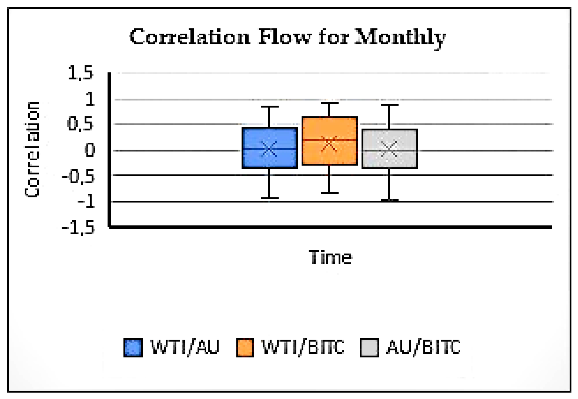
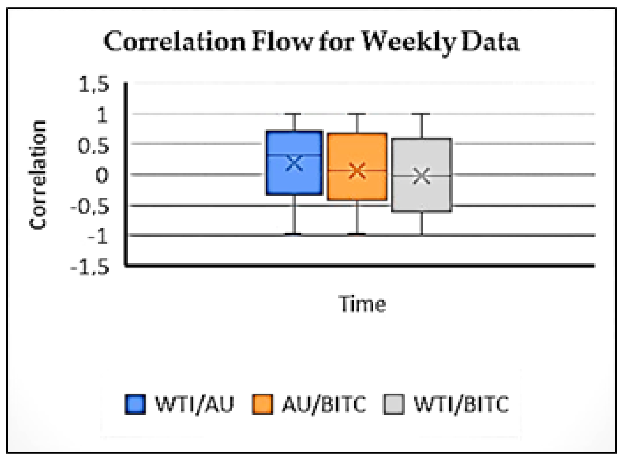
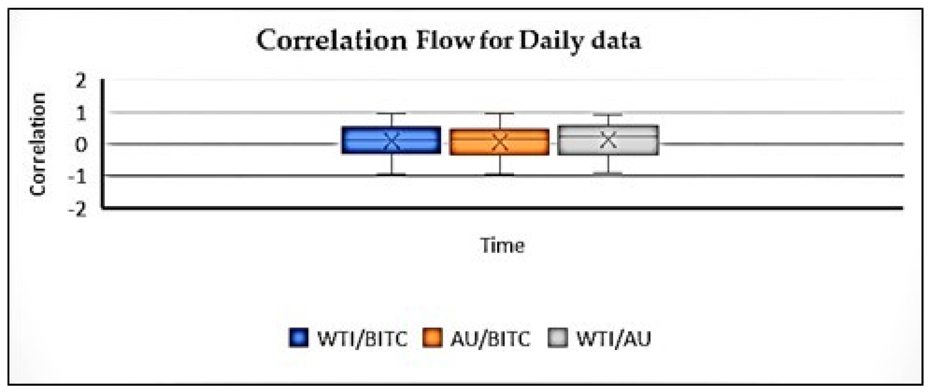
For this study, the historical daily prices of BITC, AU, and WTI were employed. The correlations were computed using a rolling window of one month. The same methodology was applied to both daily and weekly data series, but for the weekly data, 4 or 5 weeks of rolling was conducted. This was taken into account when rolling, as some months shoot 4 weeks and some 5 weeks.

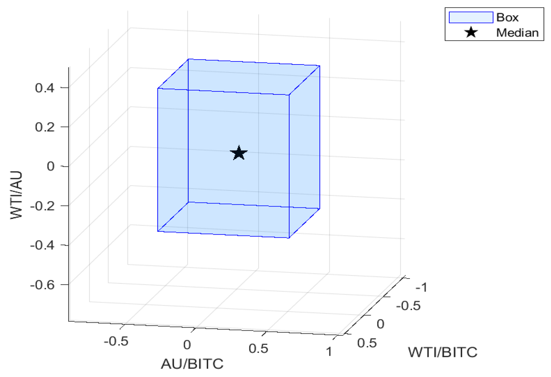
The initial covariance and orthogonal matrices obtained from the analysis are presented below:

For monthly data,

$$Po=\left[\begin{array}{ccc}0.110432& -0.020405& -0.00726\\ -0.02040& 0.467720& -0.01239\\ -0.00726& -0.01239& 0.42145\end{array}\right], H=\left[\begin{array}{ccc}0.009027& -0.00533& -0.0039\\ -0.00537& 0.52672& -0.04519\\ -0.00393& -0.0451& 0.56805\end{array}\right]$$

For Weekly Data

$$Po=\left[\begin{array}{ccc}0.106& -0.00857& 0.01788\\ -0.0085780& 0.48378& 0.0057401\\ 0.0178882& 0.0057401& 0.5138030\end{array}\right], H=\left[\begin{array}{ccc}0.0084364& 0.001485& 0.001485\\ 0.00148596& 0.516063& -0.0110\\ -0.00140& -0.0110& 0.4855\end{array}\right]$$

For Daily Data

$$Po=\left[\begin{array}{ccc}0.4962405& -0.0058469& 0.006448\\ -0.005846& 0.50157548& -0.006659\\ 0.0064483& -0.006659& 0.499019\end{array}\right], H=\left[\begin{array}{ccc}0.0022515& -0.001671& -0.001671\\ -0.000751& -0.005774& 0.004684\\ 0.004432& -0.003143& 0.010505\end{array}\right]$$

Figure 2, Figure 3 and Figure 4 show time-dependent correlation flow for monthly, weekly, and daily data.

Figure 5, Figure 6 and Figure 7 show time-dependent correlation flow for monthly, weekly, and daily data in 3D.

Robustness Check

While the time-dependent correlation flow was created for the daily data, the conversion was made for one month of working days. Only business days were included in the analysis, subtracting holidays.

Table 8. Correlation matrix among variables for daily, weekly, and monthly data.

Standard Method Weekly
	Cov. Matrix			Corr. Matrix			Spearman Cov. Matrix			Spearman Corr. Matrix
	BITC	AU	WTI	BITC	AU	WTI	BITC	AU	WTI	BITC	AU	WTI
BITC	5235910.20	3049327.55	180621.50	1	0.063	0.219	38646.63	−6532.94	11587.57	1	−0.169	0.299
AU	3049327.55	443345403.27	5935288.63	0.063	1	0.784	−6532.944	38645.74	22343.88	−0.169	1	0.578
WTI	180621.504	5935288.63	129142.11	0.219	0.784	1	11587.547	22343.88	38646.39	0.299	0.578	1
Monthly
	Cov. Matrix			Corr. Matrix			Spearman Cov. Matrix			Spearman Corr. Matrix
	AU	BITC	WTI	AU	BITC	WTI	AU	BITC	WTI	AU	BITC	WTI
AU	127664.043	−32496.050	175151.132	1	−0.342	0.214	2268.606	−279.027	700.533	1	−0.122	0.308
BITC	−32496.050	47415.881	−34555.945	−0.342	1	−0.069	−279.027	2268.642	48.221	−0.1229	1	0.021
WTI	175151.132	−34555.945	5217193.894	0.214	−0.069	1	700.533	48.221	2268.666	0.308	0.021	1
Daily
	Cov. Matrix			Corr. Matrix			Spearman Cov. Matrix			Spearman Corr. Matrix
	BITC	WTI	AU	BITC	WTI	AU	BITC	WTI	AU	BITC	WTI	AU
BITC	28219300.54	−557830.032	1373468.23	1	−0.044	0.791	1057256.984	−322588.127	529270.854	1	−0.044	0.791
WTI	−557830.03	5677766.06	158457.821	−0.04	1	0.203	−322588.127	1057320.08	306976.746	−0.044	1	0.203
AU	1373468.23	158457.821	106574.763	0.791	0.203	1	529270.854	306976.746	1057315.68	0.791	0.203	1

shows the results obtained from the standard method.

For robustness checks of the proposed model, both the standard correlation and covariance matrices, as well as the Spearman correlation and covariance matrices, were calculated using daily, weekly, and monthly data.

In

Table 9. Lie method and standard method correlation.

Lie Method				Standard Method
	Corr. Matrix			Corr. Matrix
Daily
	BITC	WTI	AU	BITC	WTI	AU
BITC	1	0.187	−0.273	1	−0.044	0.791
WTI	0.187	1	0.206	−0.04	1	0.203
AU	−0.273	0.206	1	0.791	0.203	1
Weekly
	BITC	AU	WTI	BITC	AU	WTI
BITC	1	−0.0094	−0.301	1	0.063	0.219
AU	−0.0094	1	0.228	0.063	1	0.784
WTI	−0.301	0.228	1	0.219	0.784	1
Monthly
	AU	BITC	WTI	AU	BITC	WTI
AU	1	−0.0568	0.182	1	−0.342	0.214
BITC	−0.0568	1	0.049	−0.342	1	−0.069
WTI	0.182	0.049	1	0.214	−0.069	1

, the correlation results of the standard method and those of the Lie method are shown in the same table.

The results were different from each other, which is what we expected. The following inferences from Table 9 were obtained:

1-In cases where there are fractures, long-term dependence, and chaotic characters, standard models produce results with extreme deviations.

2-In case of breaks, the correlation should be calculated following the solution of the stochastic equation using the Lie method.

3-In real life, data should be broken. Chaos, fractionality, and uncertainty is inevitable. In this case, it limits the use of the standard method.

The last comparison was made for the forecast results. The correlation flow was calculated for both methods, and the forecast successes were evaluated. Forecast successes are important to determine the success of methods. To assess the predictive accuracy of the correlation flows derived from the empirical density functions of the historical data, RMSE, MAE, and MAPE values were calculated and compared in

Table 10. RMSE, MAE, and MAPE results.

	RMSE		MAE	MAPE
Lie Method
For daily data	0.63		0.43	5.04
For weekly data	0.78		0.56	70.28
For monthly data	0.081		0.06	7.39
Standard Method
For daily data	183.43		153.28	9.88
For weekly data	98.45		71.64	7.06
For monthly data	317.77		245.40	15.62

.

When the RMSE, MAE, and MAPE values determined for the Lie method and the RMSE, MAE, and MAPE values determined by the standard method are compared for daily, weekly, and monthly data, it is seen that the RMSE, MAE, and MAPE values are very high for the standard model.

4. Discussion

This study provides the first empirical implementation and theoretical proposal of the SO(3) Lie method to obtain time-dependent correlation flows among variables with chaotic structures. While the SO(2) Lie method has been applied in previous works to model time-dependent correlation flows, our work is the first to extend this approach to three chaotic time series—Bitcoin (BITC), crude oil (WTI), and gold (AU).

Standard correlation techniques, widely applied across disciplines such as finance and engineering, may yield very high correlation coefficients when the data exhibit fractal or chaotic dynamics. Accordingly, our results, Hurst exponent analysis and Lo’s rescaled range tests, the Lyapunov exponents (calculated via Wolf, Rosenstein, and Kantz methods), Hurst exponent, entropy (Shannon, Rényi, Tsallis, HFT, HCT), and Kolmogorov–Sinai complexity scores explore the presence of chaos, long memory, and fractal and dependency characteristics in the selected variables. The positive Lyapunov exponents identified in the analysis confirm the presence of chaotic behavior in the system. The magnitude of these exponents indicates the intensity of the chaotic dynamics, providing further evidence that price movements in the dataset are sensitive to initial conditions and fundamentally unpredictable. Moreover, Hurst exponent analysis and Lo’s rescaled range tests reveal non-random and long-term dependence behaviors consistent with fractional dynamics.

Lie method time-dependent correlation matrices not only satisfy the essential mathematical properties of real symmetry and positive semi-definiteness but also reflect the stochastic nature of correlation dynamics. The results showed the importance of time-dependent correlation flow and Lie SO(3) correlation method. The robustness check results we obtained in the last stage also confirm these results. The robustness checks for different time periods (daily and weekly) show that the SO(3) Lie method outperforms better results than the standard correlation matrix method.

In standard methods, when the initial conditions change, the deviation in the results is large, but in the proposed method, this deviation is smaller because it is studied locally. This is a very important result, because according to the results we obtained from the Chaos tests and complexity measurements, the variables exhibit extreme sensitivity and complexity to the initial conditions. For this reason, the proposed method, unlike the standard method, reduces the sensitivity to initial conditions. Significance of this result can also be seen from the RMSE, MAE, and MAPE results. These values are too small for the proposed method. It delivers lower RMSE and MAPE values, greater stability, and better alignment with empirically observed shifts in asset relationships. This work accentuates how standard methods are inadequate in the presence of chaos and the SO(3) Lie method emerge as a significant step in capturing the true states of modern financial systems. And lastly, we have some practical implications for portfolio managers and risk analysts and policy makers. Our findings show several important implications for financial practice. Firstly, the proposed SO(3) Lie method can be used by portfolio managers and risk analysts to improve diversification and asset allocation strategies. Since the method captures nonlinear and chaotic structures more effectively than the standard correlation method, it can help investors reduce exposure to hidden risks that emerge during turbulent market conditions. Secondly, policymakers and regulators may benefit from this method in monitoring systemic risk and financial contagion, because correlation flows obtained by the SO(3) method provide early warning signals of instability. Thirdly, financial institutions could integrate the method into stress-testing procedures, where nonlinear interdependencies and abrupt regime shift among assets must be taken into account for more accurate scenario analysis.

Moreover, the calibration of the model to high-frequency or high-dimensional data can be technically demanding. Adoption may also face barriers in practice, because financial institutions often rely on standard correlation methods that are easier to interpret but less accurate.

5. Conclusions

This study aims to estimate the correlation flow by using the SO(3) Lie method for variables characterized by fractal and chaotic structures. The period covers from 11 April 2011 to 31 December 2024 for daily data; from 10 April 2011 to 29 December 2024 for weekly data; and from April 2011 to December 2024 for monthly data. In the first step, we investigated the data by including nonlinearity, stationarity, chaos, fractality, entropy, and complexity. These tests were conducted both on the original level data and their first differences to ensure robustness.

This paper introduces and provides an important methodological framework for estimating time-varying correlations among multiple chaotic financial variables. In contrast to the methods that assume linearity and stationarity, the SO(3) Lie method accommodates the inherent complexity and unpredictability. The SO(3) Lie method suggests that correlation flows should be actively modeled and monitored in structure where chaos exists. The SO(3) Lie method presents a rigorous method to address these challenges by bridging the gap between mathematical theory and empirical financial complexity.

For investors, policymakers, and risk managers, the results show that ignoring the nonlinear and chaotic structure of financial systems may lead to misleading estimates and investment decisions. In systems dominated by unpredictability and chaos, reliance on linear correlation estimates can lead to inefficient capital allocation, flawed risk assessments, and misguided policy responses. Our findings strongly support the incorporation of advanced modeling tools; the SO(3) Lie method—into the analytical method of financial institutions, particularly in the context of portfolio management, hedging strategies and systemic risk monitoring.

The findings from the complexity, entropy, and fractal analyses determine several important results for policymakers, investors, and risk managers. Firstly, the results found in Bitcoin, gold, and oil suggest that risk assessment and portfolio diversification strategies should consider time-horizon-specific behaviors.

Secondly, the superiority of the SO(3) Lie-based correlation flow method accentuates the need for advanced geometric and nonlinear tools in monitoring systemic risk and intermarket connections under high volatility and fractal market conditions.

Finally, the results in Bitcoin and gold accentuate that long-term investment strategies can explain structural regularities, while the entropy and irregularity of crude oil necessitate more adaptive and short-term hedging approaches. These results provide a more nuanced structure for decision making by enabling players to manage uncertainty and market complexity more effectively.

Future Research Directions and Implications

Looking forward, this paper opens several ways for future research. Extending the SO(3) framework to higher-dimensional Lie groups such as SO(n) could enable methods for larger portfolios and more complex financial systems. Combining the method with machine learning algorithms may further enhance scalability. Additionally, applying the suggested method to historical crises or market shocks can provide valuable results of its predictive capacity for the real world.