Article

An Approximate Belief Rule Base Student Examination Passing Prediction Method Based on Adaptive Reference Point Selection Using Symmetry

1
School of Computer Science and Information Engineering, Harbin Normal University, Harbin 150025, China
2
School of Computer and Mathematics, Harbin Finance University, Harbin 150030, China
*
Authors to whom correspondence should be addressed.
These authors contributed equally to this work.
Symmetry 2025, 17(10), 1687; https://doi.org/10.3390/sym17101687
Submission received: 26 August 2025 / Revised: 24 September 2025 / Accepted: 1 October 2025 / Published: 8 October 2025

Abstract

Student exam pass prediction (EPP) is a key task in educational assessment and can help teachers identify students’ learning obstacles in a timely manner and optimize teaching strategies. However, existing EPP models, although capable of providing quantitative analysis, suffer from issues such as complex algorithms, poor interpretability, and unstable accuracy. Moreover, the evaluation process is opaque, making it difficult for teachers to understand the basis for scoring. To address this, this paper proposes an approximate belief rule base (ABRB-a) student examination passing prediction method based on adaptive reference point selection using symmetry. Firstly, a random forest method based on cross-validation is adopted, introducing intelligent preprocessing and adaptive tuning to achieve precise screening of multi-attribute features. Secondly, reference points are automatically generated through hierarchical clustering algorithms, overcoming the limitations of traditional methods that rely on prior expert knowledge. By organically combining IF-THEN rules with evidential reasoning (ER), a traceable decision-making chain is constructed. Finally, a projection covariance matrix adaptive evolution strategy (P-CMA-ES-M) with Mahalanobis distance constraints is introduced, significantly improving the stability and accuracy of parameter optimization. Through experimental analysis, the ABRB-a model demonstrates significant advantages over existing models in terms of accuracy and interpretability.

1. Introduction

Student examination outcome prediction (EPP) is an important task in educational assessment that aims to predict students’ final examination results by analyzing their characteristics [1]. Its educational value mainly lies in two aspects: first, it can provide data support for personalized teaching and achieve precise teaching intervention; second, it can promptly identify students with academic difficulties and implement early warnings. In recent years, with the popularization of machine learning technology, researchers have attempted to develop EPP systems based on machine learning (ML) [2,3,4], but these methods generally have problems such as the insufficient reliability of prediction results and opaque decision-making processes, which may lead to educational ethical risks. However, most existing ML-based EPP models mainly focus on improving prediction accuracy. The interpretability and transparency of the decision-making process are neglected. A “black box” problem is caused by this. Their practical application in educational environments is limited. In addition, current methods often rely heavily on large-scale datasets. Adaptability to educational environments with small samples or dynamic changes is lacking. Their generalization ability and real-time response capability are restricted. A significant gap also exists in the integration of domain knowledge and data-driven methods. As a result, the models are neither fully credible nor pedagogically informative. Given the rapid development of artificial intelligence technology [5], constructing an EPP model with high accuracy and strong interpretability is particularly important [6,7,8,9].
In recent years, various machine learning methods have been applied in the field of student EPP [10]. Early studies mainly employed machine learning techniques, such as those of Kabakchieva et al. [2], who compared the application of three typical algorithms—decision tree, K-nearest neighbor, and neural network—in the field of higher education and verified the applicability of machine learning in this problem. With the demand for higher prediction accuracy and more complex data processing, subsequent studies began to explore advanced model architectures and innovative estimation methods. Cao et al. [11] proposed a novel hierarchical probabilistic neural framework, which combines Bayesian inference with symmetric deep neural architectures to achieve adaptive and efficient knowledge assessment. Triveni et al. [12] introduced two innovative estimators aimed at assessing the finite population distribution function of the research variable. They utilized auxiliary variables within the framework of stratified random sampling and post-stratification, while emphasizing symmetry in the sampling process. While these architectural innovations improved model performance, researchers gradually noticed practical limitations in real-world educational scenarios, prompting investigations into the shortcomings of existing methods. Wang et al. [13] conducted research on predicting university academic achievements by applying interpretable models, verifying the effectiveness of machine learning methods in this field, but found that existing models had prediction limitations due to their excessive reliance on historical static data. Vytautas et al. [14] used multi-sensor methods to process examination pressure data collected by wearable devices to predict academic performance, verifying the feasibility of this method in performance prediction, but found that it had value assessment limitations due to the lack of comparative studies with traditional prediction methods. To address the ambiguity of “which basic algorithm performs better in educational scenarios”, researchers conducted systematic comparisons of classic machine learning algorithms. Khairy et al. [15] compared the performance of various machine learning algorithms, such as random forest, decision tree, naive Bayes, neural network, and K-nearest neighbor, on educational datasets, verifying the superior performance of random forest and decision tree classifiers. While algorithm comparisons identified more effective models, the pursuit of personalized educational assessment led researchers to rethink the problem itself, shifting from traditional “performance prediction” to a more scenario-adapted paradigm. Other scholars innovatively transformed the student performance prediction problem into a recommendation system problem [16,17] in an attempt to achieve more personalized prediction solutions. Notably, these methods essentially belong to the data-driven paradigm, and the performance of their models largely depends on large-scale training samples. Therefore, in cases of limited sample sizes, it is often difficult to achieve ideal results.
In EPP research, the existing methods can be classified into three main categories: data-driven methods, knowledge-driven methods, and hybrid-driven methods that combine the advantages of both. Data-driven predictive models demonstrate high accuracy on large datasets, but this advantage often comes at the expense of model interpretability. As the prediction accuracy of the model increases, its internal mechanism tends to become more complex and difficult to understand, which not only increases the difficulty for educators in interpreting the prediction results but also may lead to an information gap between developers and users, thereby causing issues related to educational equity. In contrast, knowledge-driven methods, although theoretically more interpretable, often have difficulty significantly improving their prediction accuracy, especially in handling data uncertainty. When faced with imperfect data collection techniques, fluctuations in learners’ environmental factors and psychological states further affect the stability of measurement results, which challenges the reliability of knowledge-driven methods [18]. On the basis of these two driving methods, researchers have proposed a hybrid driving method that integrates domain expert experience and historical data organically, ensuring prediction performance while balancing the accuracy and interpretability of the model well.
The belief rule base (BRB) is a hybrid-driven modeling method that has unique advantages in balancing model prediction accuracy and interpretability [19]. This model integrates fuzzy reasoning theory, IF-THEN rule systems, and ER methods and can effectively handle uncertainties in the data collection and analysis process [20,21]. In the field of educational research, Chen et al. [22]. successfully applied the BRB framework to construct a learning emotion assessment model, and its performance was significantly superior to that of ML models. Notably, the BRB method, owing to its rule-based modeling nature, has prominent advantages in terms of model transparency and decision interpretability. This study is based on the core principles of the BRB method and focuses on exploring its innovative application in the EPP teaching method.
Although the BRB model has unique advantages in EPP system modeling, its application in actual teaching scenarios still faces multiple challenges. First, the model constructed on the basis of limited expert knowledge has difficulty comprehensively depicting the dynamic characteristics of complex teaching systems. Second, the traditional BRB structure has insufficient adaptability to the time-varying characteristics and multimodal distribution in teaching data. Third, static optimization methods cannot meet the continuous parameter adjustment requirements of the dynamic teaching environment. Most importantly, the existing models lack effective mechanisms to balance prediction accuracy and structural complexity. These limitations indicate that systematic improvements need to be made to the traditional BRB from multiple dimensions, such as the model structure, optimization algorithm, and balance strategy, to enhance its applicability in dynamic teaching environments.
Therefore, this paper proposes an approximate belief rule base EPP model (ABRB-a) based on adaptive selection of symmetrical reference points. The main contributions of this paper are as follows:
(1) To address the issue of effective screening of multi-source heterogeneous features in the EPP task, a random forest method based on cross-validation was adopted, incorporating intelligent data cleaning, adaptive tree structure tuning, and multi-fold validation strategies to achieve precise screening of multi-dimensional features.
(2) To reduce the dependence of EPP model construction on domain prior knowledge, a clustering method with an agglomerative nature was introduced to automatically generate reference points, effectively overcoming the limitations of traditional methods that rely on expert experience. Additionally, a model reasoning mechanism based on ER rules was constructed to ensure the interpretability and transparency of the decision-making process.
(3) Facing the problem of a difficult balance between model accuracy and complexity in the high-dimensional parameter space of EPP, an innovative optimization algorithm with Mahalanobis distance constraints, P-CMA-ES-M, was adopted. Under the control of model complexity, parameter adaptive optimization was achieved, significantly improving the accuracy and generalizability of exam pass prediction.
The remainder of this article is organized as follows. In Section 2, the problem is described. In Section 3, the EPP model based on ABRB-a is constructed. The reference point generation process, reasoning process, and optimization process introducing the Mahalanobis distance of the model are introduced. In Section 4, experimental verification of the ABRB-a model is carried out. In Section 5, the conclusion is given. Finally, in Section 6, the explanations for all the letters are provided.

2. Problem Description

This section identifies the core challenges involved in building the EPP model. The EPP model constructed based on ABRB-a needs to address the following issues:
Problem 1: How to accurately obtain the initial modeling parameters of the ABRB-a model.
In the ABRB-a model, each rule is composed of three core parameters: the attribute reference point, the attribute weight, and the rule weight. Determining these parameters is a key step in the construction of the ABRB-a model. However, when domain expertise is insufficient, the initialization of model parameters faces significant challenges.
To address this key issue, this study proposes an adaptive reference point extraction method based on data mining. By mining the underlying patterns in a large amount of educational data, the optimal reference points are automatically extracted. However, there is an important trade-off relationship between the number of reference points and model performance. Too many reference points lead to a significant increase in model complexity, whereas too few reference points reduce model accuracy. Therefore, the process of obtaining initial parameters is defined as follows:
Q = F ( α , φ )
Here, Q represents the initial parameters of the ABRB-a model, F ( α , φ ) indicates the data mining process, α represents the historical data, and φ indicates the data mining parameters.
Problem 2: Optimizing the parameters of ABRB-a to increase the model’s accuracy.
The ABRB-a model possesses both nonlinear modeling capabilities and good interpretability. Its initial parameters are usually set by domain experts based on their experience. However, this method, which is based on experience, has subjective uncertainties, which may lead to suboptimal parameter settings. To improve the model’s accuracy, this study employs the P-CMA-ES-M algorithm with constraints to systematically optimize these parameters. The specific optimization process is as follows:
Q b e s t = G ( L , P )
Here, Q b e s t represents the optimization parameters of the ABRB-a model, G ( L , P ) indicates the model optimization process, and L represents the parameters of P-CMA-ES-M.
Problem 3: How can a reasonable ABRB-a model be constructed when there are too many attributes?
The traditional BRB model generates rules via the Cartesian product method. When there are many input attributes, the combinatorial explosion problem occurs, resulting in an exponential increase in the number of rules. This phenomenon of rule proliferation not only significantly increases the complexity of the model but also leads to dimension disasters, significantly reducing the computational efficiency and prediction performance of the model. To solve this problem, the following nonlinear mapping relationship was designed:
y = P ( X ˜ , Q )
Here, y represents the prediction result of the model. Q represents the initial parameters set by the experts. X ˜ = x ˜ 1 , x ˜ 2 , , x ˜ M is the input feature set, which represents the M prerequisite attributes of the model. y = ( · ) indicates the nonlinear functional relationship between the system characteristics and the predicted value.

3. Construction of the EPP Model Based on ABRB-A

This section will construct the model through the following five subsections. In Section 3.1, the theory and advantages of the model design are analyzed. In Section 3.2, the overall architecture construction process of the model is described. In Section 3.3, the dynamic generation mechanism and construction method of the reference points are introduced. Section 3.4 describes the reasoning process of the ABRB-a model. The parameter optimization of the ABRB-a model is described in Section 3.5. In Section 3.6, the algorithm is analyzed accordingly.

3.1. Theoretical Basis and Advantages of Model Design

In terms of the model design principle, this study adopts a “hybrid-driven” approach. This approach is consistent with the core logic of Chen et al. [22] who applied BRB to educational emotion assessment. The advantages of the BRB method in balancing model accuracy and interpretability are verified by both. The applicability of the BRB framework in the field of educational assessment is further consolidated. Meanwhile, this study adopts a strategy of screening key features through random forests. This strategy is consistent with the conclusion verified by Khairy et al. [15] that “random forests perform excellently in educational datasets”. It shows that the selection of basic methods in this study conforms to the consensus conclusions in this field. Therefore, the overall framework and method selection of this study are consistent with existing studies. Compared with the limitations of traditional BRB models that rely on expert experience to set reference points [19,21], this study innovatively introduces a hierarchical clustering algorithm. The adaptive generation of reference points is realized through this algorithm. The dependence on domain prior knowledge is effectively reduced. At the same time, a P-CMA-ES-M algorithm with Mahalanobis distance constraint is proposed. The applicability and robustness of the model in scenarios with small samples or lack of expert experience are significantly enhanced by this improvement. This improvement is an important advancement to the existing BRB methods.
In terms of the algorithm architecture, this study innovatively proposes a four-stage progressive processing framework and constructs a complete modeling loop [23,24]. This framework first uses the random forest algorithm for feature selection, effectively eliminating redundant variables and ensuring the purity of the input feature information; then, it adopts the hierarchical clustering method to dynamically generate reference points, providing an adaptive benchmark for the decision-making process; finally, it introduces the ER mechanism to achieve transparent and interpretable decision-making reasoning in an uncertain environment; finally, it uses the P-CMA-ES-M optimization algorithm with Mahalanobis distance constraints to optimize the parameters, ensuring the global optimality of the model parameters. This “feature reduction, adaptive benchmark, interpretable reasoning, parameter optimization” progressive design not only forms a rigorous algorithmic logic chain but also mutually supports and optimizes each module, ensuring the interpretability of the model and improving the stability of the overall performance [25].
Finally, from the perspective of application value, this method achieves a balance between performance and interpretability through modular design. Each functional module can be independently verified and can also be optimized collaboratively. It not only meets the requirements of educational decision-making for model transparency but also maintains sufficient modeling flexibility.

3.2. Construction Process of the Model

Figure 1 illustrates the construction process of the EPP model based on ABRB-a. A brief modeling framework is as follows:
(1) Design of the ABRB-a model: The number of combination rules in the ABRB-a model increases linearly, solving the problem of combinatorial explosion.
(2) Reference points of the model: Hierarchical clustering-based agglomerative clustering is used to automatically generate reference points, overcoming the limitations of traditional methods that rely on expert prior knowledge.
(3) Evidential reasoning (ER) algorithm: The process is transparent, and the rules are clear, ensuring the interpretability of the reasoning process.
(4) Optimization algorithm optimization: The P-CMA-ES-M algorithm with Mahalanobis distance constraints is used to optimize the parameters of the model, improving its accuracy.
(5) Expected utility: The performance of the model is evaluated by calculating the utility value for accuracy.
To address the above three key issues, this section constructs an EPP model that is based on ABRB-a. The ABRB-a model is a modeling method that is based on IF-THEN rules. Like the traditional BRB, the ABRB-a model is also composed of a series of belief rules. Therefore, the h t h belief rule of the i t h attribute in the ABRB-a model is described as follows:
R i , h : If   X ˜ i   i s   A ^ i , h , Then   y   i s   D 1 , β 1 , i , h , , D N , β N , i , h , n = 1 N β n , i , h 1 with   a   rule   weight   θ i , h   and   the   attribute   weight   δ i   ( i = 1 , , M , h = 1 , , H i )
Here, R i , h represents the h t h belief rule, A ^ i , h is the h t h reference value of X ˜ i , β n , i , h ( n = 1 , , N ) represents the belief degree of D N , and θ i , h represents the rule weight of R i , h , indicating the weight of the h t h belief rule. δ i is the attribute weight of the premise, indicating its importance compared with other attributes.
This single-attribute rule allows for the linear growth of rules rather than combining belief rules in a Cartesian product manner, as in the BRB model. This effectively prevents the problem of rule explosion caused by excessive attributes. Through this definition, the ABRB-a model can provide a structured way to represent and explain the complex relationships in the data, making the decision-making process of the model more transparent and interpretable [26]. The characteristic of this model is that it provides a clear and transparent decision-making process while ensuring an increase in accuracy, facilitating the understanding of the basic principles of the model.

3.3. Adaptive Construction Method for Reference Points in Hierarchical Clustering

3.3.1. Introduction to Hierarchical Clustering

Hierarchical clustering is an unsupervised learning method based on a tree structure. It reveals the inherent organizational patterns of data by constructing a multi-level clustering structure. Unlike partition-based clustering, hierarchical clustering does not require prespecification of the number of clusters. Instead, hierarchical clustering results are obtained by gradually merging or splitting the dataset [27,28,29].
Depending on the direction of construction, hierarchical clustering can be divided into two main strategies: the bottom-up agglomerative method and the top-down divisive method. In this experiment, the more widely applied agglomerative clustering method was adopted. This method follows the principle of “merging first”, starting by treating each data sample as an independent cluster and, through iterative merging of the closest cluster pairs, gradually forming larger clusters [30], ultimately constructing a complete clustering hierarchy until all samples belong to the same cluster [31,32]. The specific process is shown in Figure 2.

3.3.2. Operating Procedure

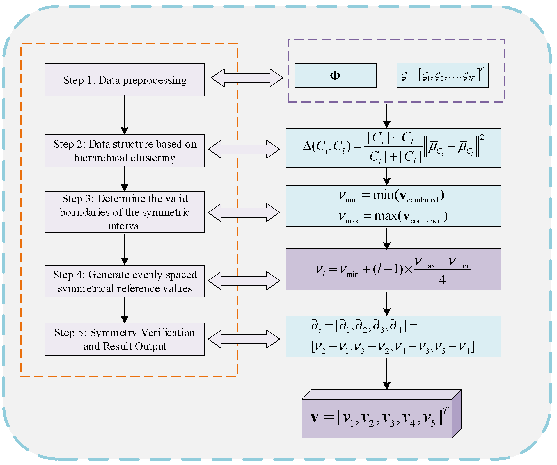
In this study, the agglomerative clustering method was employed to automatically classify the characteristic parameters, and a reference value sequence was constructed on the basis of the cluster centers. The specific process is shown in Figure 3.
Taking the data from this experiment as an example, this algorithm calculates the similarity between samples and iteratively merges the nearest neighbor clusters, ultimately automatically generating an optimized sequence consisting of 5 typical reference points. The specific implementation process mainly includes the following key steps:
Step 1: Data preprocessing
The data is stored in Excel files. The features are extracted and transformed from the table form into a numerical matrix Φ of size N × M , where a represents the sample size and b represents the number of features. For the i t h feature ( i = 1 , 2 , , M ) , the data vector ς = ς 1 , ς 2 , , ς N T is extracted.
Among them, Φ constitutes the N × M matrix of the entire dataset, and ς is a data vector representing the observed values of all samples for the i t h feature.
Step 2: Data structure based on hierarchical clustering
First, calculate the dissimilarity matrix, using Euclidean distance as the measure of dissimilarity. For any two sample points ς a and ς b , the distance is as follows:
d ( a , b ) = | ς a ς b |
Among them, ς a , ς b represents the specific sample observation values at the a t h and b t h positions within vector ς .
Then, inter-cluster links are established, using the Ward minimum variance method as the linking criterion. The calculation formula is as follows:
Δ ( C i , C l ) = | C i | | C l | | C i | + | C l | μ ¯ C i μ ¯ C l 2
This article sets the maximum number of clusters Γ = 3 , and the algorithm continuously merges clusters until the entire dataset is divided into three mutually exclusive clusters C 1 , C 2 , C 3 . Here, Γ represents the number of clusters, C i , C l indicates the i t h cluster and the l t h ( l = 1 , 2 , , L ) cluster. μ ¯ C i is the arithmetic mean of the i t h sample value within the cluster, and Δ ( C i , C l ) is the sum of squared within-cluster variances caused by merging clusters C i and C l .
Step 3: Determine the valid boundaries of the symmetric interval
In order to determine an effective range ν min , ν max that can cover the core distribution of the data and is also robust against outliers, it serves as the reference interval for generating symmetrical reference values.
First, for each cluster C Γ Γ = 1 , 2 , 3 , calculate the arithmetic mean as the cluster center μ Γ : the details are as follows:
μ Γ = 1 | C Γ | ς i C Γ ς i
Among them, μ Γ is the center of the Γ t h cluster, which is calculated based on the average of all sample values within this cluster. Then, a comprehensive vector v combined is created, including the global extremum and the center values of all clusters. As follows
v combined = min ( ς ) , μ 1 , μ 2 , μ 3 , max ( ς ) T
Among them, v combined is a comprehensive vector consisting of the global minimum value, the centers of the three clusters, and the global maximum value, which is used to determine the effective range.
Finally, the boundaries are determined. The lower bound ν min and the upper bound ν max of the effective range are, respectively, the minimum and maximum values in the comprehensive vector.
ν min = min ( v combined ) ν max = max ( v combined )
This method ensures that the effective range necessarily includes the center points of all clusters and extends to the global boundary of the data, thereby enabling the generated reference values to represent the overall distribution characteristics of the data.
Step 4: Generate evenly spaced symmetrical reference values
Within the valid interval ν min , ν max , through linear interpolation, L = 5 reference points are forcibly generated that are strictly evenly spaced numerically, achieving mathematical symmetry. The calculation formula for the l t h reference value v l is as follows:
ν l = ν min + ( l 1 ) × ν max ν min L 1
Substitute L = 5 and obtain the final five reference values:
ν l = ν min + ( l 1 ) × ν max ν min 4 , l = 1 , 2 , 3 , 4 , 5
The interval Δ between any two adjacent reference values is a constant and ensures its symmetry:
Δ = ν l + 1 ν l = ν max ν min 4 , l = 1 , 2 , 3 , 4
It ensures that the reference value sequence ν = ν 1 , ν 2 , ν 3 , ν 4 , ν 5 has strict numerical symmetry. The first point ν 1 is equal to ν min , and the last point ν 5 is equal to ν max .
Step 5: Symmetry Verification and Result Output
Calculate the difference vector of the adjacent reference values. If the conditions are met, it is determined that the reference values meet the symmetry requirement.
i = [ 1 , 2 , 3 , 4 ] = [ ν 2 ν 1 , ν 3 ν 2 , ν 4 ν 3 , ν 5 ν 4 ]
Verify the equidistant characteristic of the generated reference values and output the most symmetrical set of reference values, denoted as ν .
This study generated equidistant reference values through hierarchical clustering, initially incorporating the concept of symmetry into the basic structure of the model. However, this exploration of geometric symmetry is still at a superficial level. Future research needs to expand towards deeper symmetries driven by the intrinsic distribution of data or complex business logic.

3.4. Reasoning Process of the ABRB-A Model

In this section, after the EPP model is constructed on the basis of ABRB-a, the ER method is adopted to realize the reasoning process of the model [19]. In the proposed EPP modeling framework, the ER mechanism is designed as the basis for rule fusion in the final stage of the reasoning process [33,34]. The reasoning process follows the following rigorous steps: calculating the matching degree, determining the rule activation weights, executing the reasoning operations via the ER machine, and finally, outputting the expected utility value, thereby obtaining reliable prediction results.
Step 1: Calculate the matching degree
When the observational data are obtained, it is necessary to apply rule-based equivalent transformation technology and fuzzy membership functions to convert them into the unified format of A ^ i , h , a i , h i = 1 , , M ; h = 1 , , H i . The matching degree of x i with the rules can be calculated as follows:
a i h = θ i , h a i , h δ i
δ i = δ i max i = 1 , , M δ i
Here, δ i is used to define the normalization weight of the attributes, whereas a i h is used to define the matching degree of the h t h rule.
Step 2: Activation of the Rules Weights
Calculate the rule activation weights w i , h for these rules. The calculation method is as follows:
w i , h = a i h i = 1 , h = 1 L a i h
Step 3: ER inference engine
A single rule cannot serve as the standard for evaluating the result. The ER algorithm needs to be used for rule fusion reasoning to obtain the final belief degree β n ( n = 1 N ) . The calculation method is as follows:
β n = i = 1 , h = 1 L w i , h β n , i , h + γ n i , h i = 1 , h = 1 L γ n i , h n = 1 N i = 1 , h = 1 L w i , h β n , i , h + γ n i , h ( N 1 ) i = 1 , h = 1 L γ n i , h i = 1 , h = 1 L 1 w i , h  
γ n i , h = 1 w i , h n = 1 N β n , i , h
The belief distribution of the final result can be expressed as follows:
S ( A ) = ( D n , β n )   ;   n = 1 , , N
Step 4: Expected utility value
The calculation of the expected utility value leads to the final output result:
y ( S ( A ) ) = n = 1 N u ( D n ) β n
In the above equation, S represents the belief distribution set, A is the actual input vector, y S A is the final expected utility, and μ ( D n ) represents the utility value of D n .

3.5. Optimization Process of the ABRB-A Model

Model accuracy is one of the core indicators for measuring the performance of a model. To further increase the model accuracy, this paper conducts an in-depth analysis of the model optimization strategies. In the context of EPP model research based on ABRB-a, the accuracy of the ABRB-a model is affected not only by the reference point but also closely related to other parameters [35]. Therefore, in the model optimization process, this paper focuses on the refinement of the belief distribution and the optimization of rule weights and attribute weights, aiming to minimize the mean square error (MSE).
When the model is optimized, it is necessary to clearly define the target optimization function and ensure that this function can guide the model to continuously improve the prediction accuracy during the iterative process [36]. Moreover, the key parameters of the model (the belief degree of rules, rule weights, etc.) must strictly follow the constraints set by expert knowledge [37]. On the basis of the ABRB-a model framework, the mean square error M S E ( θ ) is used to quantify the deviation between the model’s predicted values and the actual observed values. Therefore, the optimization objective function can be expressed as follows:
min M S E ( θ i , h , β n , i , h , δ i ) s . t . 0 θ i , h 1 , 0 β n , i , h 1 , 0 δ i 1 n = 1 , 2 , N i = 1 , 2 , M h = 1 , 2 , H i
Here, θ i , h represents the interpretability constraint on the rule weights, β n , i , h represents the interpretability constraint on the belief degree, and δ i represents the interpretability constraint on the attribute weights.
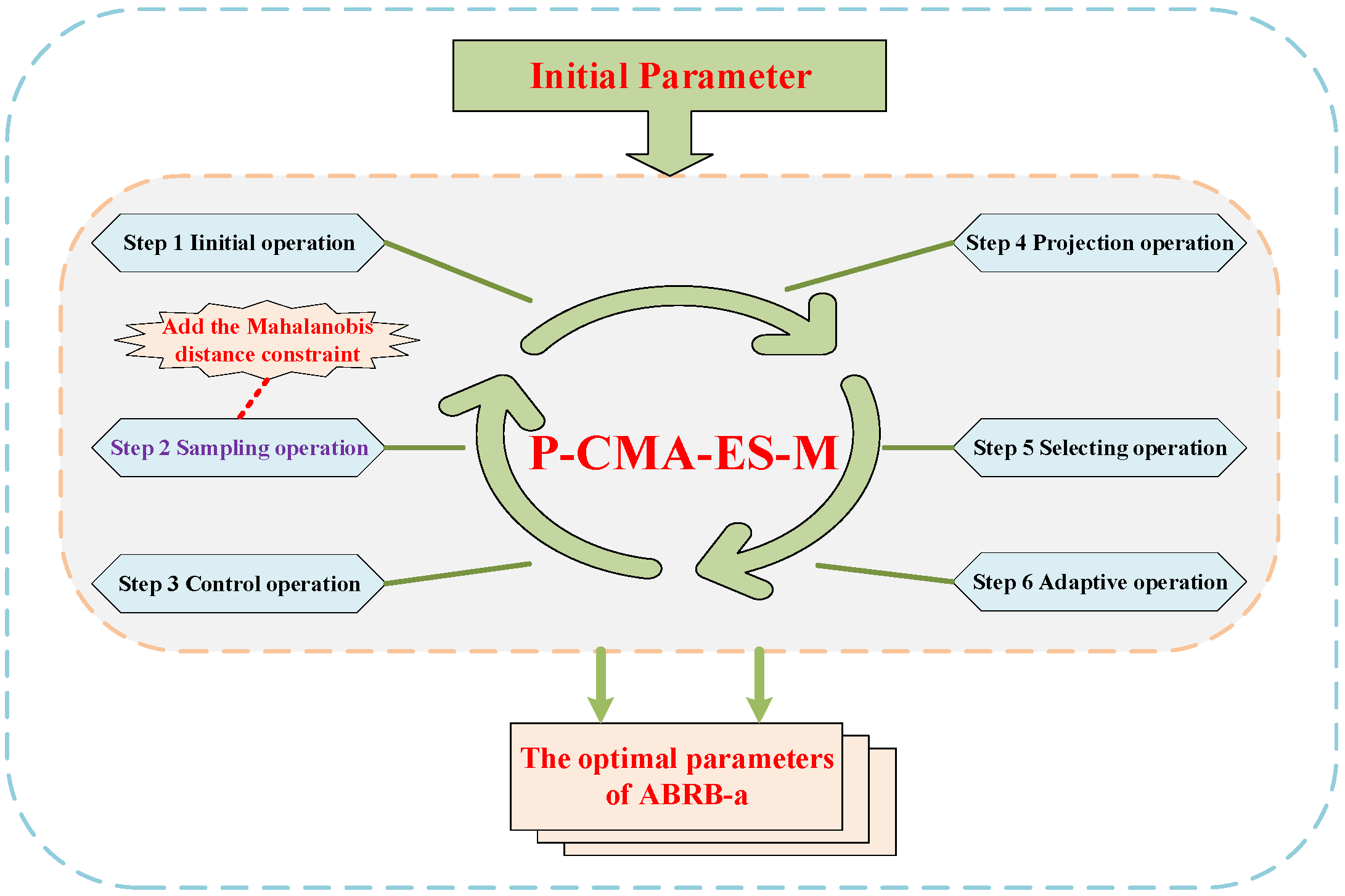
In current research, various optimization algorithms have been applied to the model optimization process. Among them, the P-CMA-ES-M algorithm performs exceptionally well in the optimization of the BRB model. This paper integrates the Mahalanobis distance constraint into this algorithm, enabling it to demonstrate more significant advantages in solving complex optimization problems, especially for adjusting the internal parameters of the BRB model, which can effectively improve the accuracy and efficiency of the model. The P-CMA-ES-M optimization process is shown in Figure 4.
The P-CMA-ES-M algorithm has the following prominent advantages: (1) strong robustness and fast convergence speed; (2) an optimization mechanism that mimics the principles of biological evolution; and (3) excellent performance when dealing with complex optimization problems. The specific steps are as follows:
Step 1: Initial operation
The parameters of P-CMA-ES-M with the Mahalanobis distance are initialized. Set the initial covariance matrix C , the population size ε , the size of the offspring population k , and the initial step size λ . The parameters to be optimized are represented as follows:
m e a n ( g ) = ψ θ 1 , 1 , , θ M , H i , β 1 , 1 , 1 , , β N , M , H i , δ 1 , , δ M
Here, m e a n ( g ) represents the mean value of the best overall performance in the g t h generation. ψ represents the parameter set.
Step 2: Sampling operation
The initial overall structure is generated through constraints with the Mahalanobis distance:
Ω k ( g + 1 ) = m e a n ( g ) + λ ( g ) D M ( g ) N ( 0 , C ( g ) ) , k = 1 , 2 , , ε s . t . D M ( Ω k ( g + 1 ) , m e a n ( g ) ) d
Here, β n , i , h g + 1 represents the generation of a reasonable belief distribution in the ( g + 1 ) t h generation. N · is a normal distribution. D M represents the Mahalanobis distance and d represents the distance.
Step 3: Control operation
Identify and resample the incorrect belief distribution Ω k g + 1 until they all meet the following distribution conditions:
Ω k g + 1 β n , i , h g + 1 = m e a n g + ε g N 0 , C g β n , i , h g + 1 I D , k = 1 , 2 , , λ
Ω k g + 1 is the k t h solution in the ( g + 1 ) t h generation and may contain incorrect belief distributions. It is a newly created belief distribution that satisfies ID. The symbol represents the replacement operation, which can replace the incorrect belief distribution in Ω k g + 1 .
Step 4: Projection Operation
To satisfy the equality constraints, the equality constraints are transformed into equality constraints on the hyperplane via the projection operation. The specific procedure is as follows:
A e Ω k g + 1 1 + n e × j 1 : n e × j = 1
The implementation method of the projection operation is as follows:
Ω k g + 1 1 + n e × j 1 : n e × j = Ω k g + 1 1 + n e × j 1 : n e × j A e T × A e × A e T 1 × Ω k g + 1 1 + n e × j 1 : n e × j × A e
A e represents the parameter vector, n e represents the number of parameters, and j represents the number of equation constraints included in the constraints.
Step 5: Select the operation
The optimal solution is chosen from the overall set ψ , and the mean value is updated. The selection operation is carried out via the following formula:
m e a n g + 1 = k = 1 λ ω k Ω k : ε g + 1
ω k represents the weight coefficient.
Step 6: Adaptive operation
The covariance matrix of the population is updated via the following two formulas:
C g + 1 = 1 c 1 c 2 × C g + c 1 p c g + 1 p c g + 1 T + c 2 k = 1 τ ω k Ω k : ε g + 1 m e a n g λ g Ω k : ε g + 1 m e a n g λ g T
p c g + 1 = 1 C c × p c g + C c 2 C c × k = 1 τ ω k 2 0.5 × m e a n g + 1 m e a n g / λ g
Here, τ represents the intermediate variable, c represents the learning rate, p c represents the evolution path of the covariance matrix, and C c represents the backward time range of the evolutionary path.
The step length λ is updated via the following two formulas:
λ g + 1 = λ g exp c σ d σ | | p σ g + 1 | | G | | N 0 , Ι | | 1
Here, d σ is the damping coefficient, G N 0 , Ι represents the expected value of the Euclidean norm N 0 , Ι , Ι represents the identity matrix, c σ represents the parameters of the conjugate evolution path p c , and p c is updated according to the following formula:
p c g + 1 = 1 C c × p σ g + C c 2 C c × k = 1 τ ω k 2 0.5 × C g 0.5 × m e a n g + 1 m e a n g / λ g
Step 7: Repeat this process iteratively until an optimal solution is reached.

3.6. Analysis Related to Algorithms

3.6.1. ABRB-A Student Exam Pass Prediction Pseudo-Code

Pseudocode is Algorithm 1 below. The steps are described as follows:
Step 1: Build the ABRB-a model. Firstly, initialize the model based on the belief rules defined by expert knowledge. Then, determine the set of input attributes based on the feature selection results, and effectively avoid the rule combination explosion problem existing in the BRB model by designing a linearly growing rule generation mechanism.
Step 2: Adaptive reference point generation. For each input attribute, a hierarchical clustering algorithm is used to analyze the data distribution characteristics. Then, symmetrical reference points are automatically generated, and the validity of the symmetry of these generated reference points is verified.
Step 3: Evidence reasoning process. For each input data instance, first calculate the matching degree between it and each reference point, and then determine the activation weight of the corresponding rule based on the matching result; subsequently, execute the evidence reasoning algorithm to achieve the effective integration of multiple rules, and finally output the belief distribution reflecting the possibility of the student’s examination results.
Step 4: Model parameter optimization. Firstly, the model parameters are initialized based on expert knowledge. Subsequently, the P-CMA-ES-M optimization algorithm with the introduction of Mahalanobis distance constraints is employed to systematically optimize key parameters such as belief degree, rule weights, and attribute weights, while ensuring that all parameter adjustments meet the requirements of model interpretability constraints.
Step 5: Model Evaluation. Input the test dataset into the optimized ABRB-a model. Calculate the expected utility value for each test instance based on its success/failure, and compare the predicted results with the actual labels for analysis. Finally, comprehensively evaluate the model’s predictive performance by integrating accuracy rate and other performance indicators.
Algorithm 1 Pseudocode for ABRB-a Student Examination Passing Prediction Model
//Step 1: Build the ABRB-a Model
Initialize the ABRB-a model with expert-defined belief rules
Initialize input attribute set based on feature selection results
Ensure linear growth of rules to avoid combinatorial explosion
//Step 2: Adaptive Reference Point Generation
For each input attribute:
   Apply hierarchical clustering algorithm to analyze data distribution
      Automatically generate symmetric reference points
         Validate the symmetry of generated reference points
//Step 3: Evidence Reasoning Process
For each input data instance:
   Calculate matching degree between input and reference points
      Determine rule activation weights based on matching results
Execute evidence reasoning for rule fusion
Output belief distribution for pass/fail prediction
//Step 4: Model Parameter Optimization
Initialize model parameters with expert knowledge
   Apply P-CMA-ES-M algorithm with Mahalanobis distance constraints
      Optimize belief degrees, rule weights, and attribute weights
Ensure parameters satisfy interpretability constraints
//Step 5: Model Evaluation
Input test dataset to the optimized ABRB-a model
For each test instance:
   Calculate expected utility value for pass/fail prediction
      Compare predicted results with actual labels
Evaluate model performance using accuracy and other metrics
//Output the final prediction results and model performance
End

3.6.2. Complexity Analysis

The complexity mainly stems from the following core operations:
(1) Sampling operation complexity: In each generation, the algorithm needs to generate k offspring individuals. The generation of each individual involves the decomposition operation of the covariance matrix, whose time complexity is O ξ 3 , where ξ is the dimension of the parameters to be optimized. Therefore, the total complexity of the sampling operation is O k ξ 3 .
(2) Complexity of fitness evaluation: Each individual needs to undergo fitness calculation through the ABRB-a model. Assuming that the time complexity of model inference is O H i M , where H i represents the number of rules and M represents the number of attributes. Therefore, the complexity of population fitness evaluation is O k H i M .
(3) Projection operation complexity: To satisfy the equality constraints, the algorithm needs to perform projection operations on illegal solutions. The time complexity of calculating the projection matrix is O κ ξ 2 , where κ represents the number of equality constraints. The complexity of each individual’s projection operation is O ξ 2 .
(4) Complexity of covariance matrix update: The update of the covariance matrix involves rank-1 update operations, and its complexity is O ξ 2 . The update complexity of the evolutionary path is O ξ .
Overall complexity: Let the maximum number of iterations be G. Then, the total time complexity of the P-CMA-ES-M algorithm can be expressed as follows:
O G k ξ 3 + k H i M + k ξ 2 + ξ 2
Since usually ξ 2 k ξ 3 is present and H i M is a constant term, the dominant term of the algorithm is O G k ξ 3 .

4. Case Study

Section 4.1 provides a background description. The model settings of ABRB-a are described in Section 4.2. The experimental results are presented in Section 4.3. A comparative experiment is conducted in Section 4.4. In Section 4.5, the generalization verification is presented. The experimental summary is given in Section 4.6.

4.1. Background Description

The dataset used in this experimental case is from https://www.kaggle.com/datasets/amrmaree/student-performance-prediction (accessed on 30 September 2025).
This dataset contains seven attributes: gender (G), Study Hours Per Week (SHPW), Attendance Rate (AR), Past Exam Scores (PES), Parental Education Level (PEL), Internet Access at Home (IAH), Extracurricular Activities (EA). There is also a binary classification result label (Pass/Fail). These features comprehensively cover the personal, family and learning behavior factors that may affect academic performance, providing a reliable data foundation for subsequent analysis.
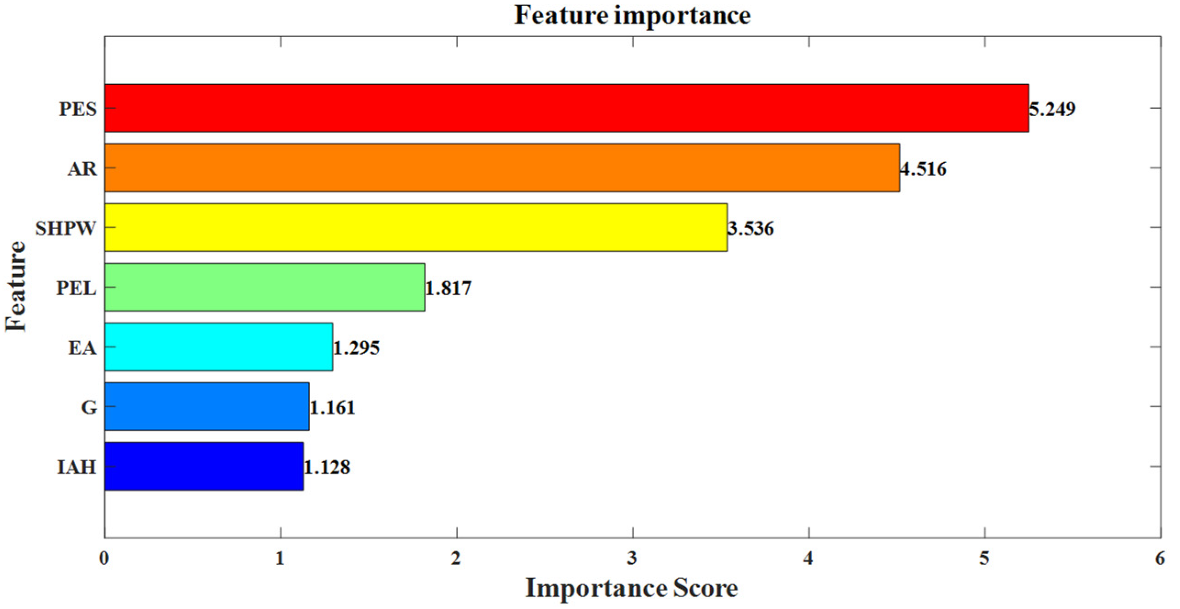
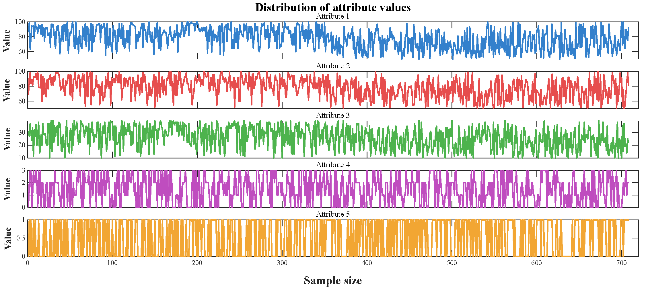
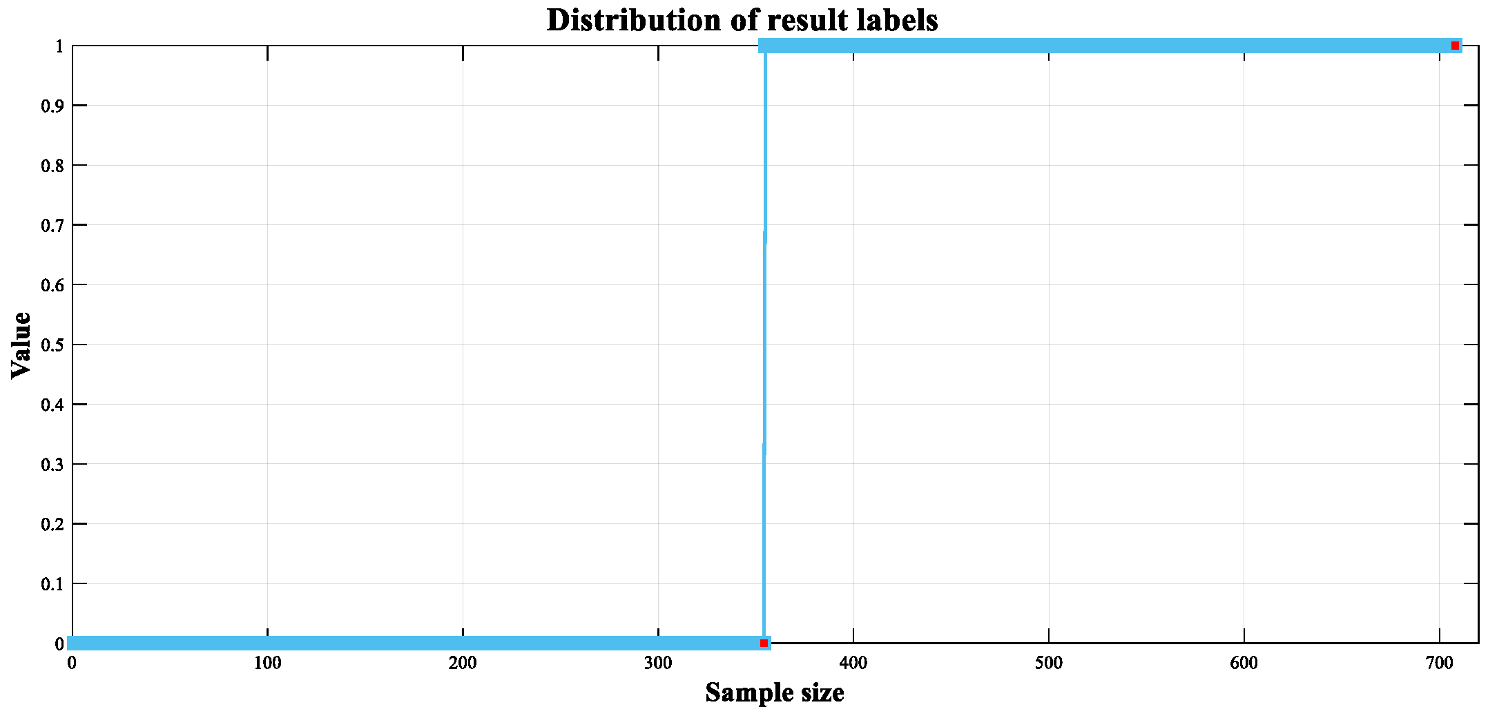
As shown in Figure 5, the feature importance analysis result based on the random forest algorithm indicates that among the seven features, the feature that has the greatest impact on the prediction result is the past academic performance (PES), whereas the influence of sex (G) is relatively minimal. According to the importance ranking, the first five key features are selected as the input variables for the subsequent analysis. Figure 6 shows the distribution of these five features, whereas Figure 7 presents the distribution statistics of the result label (Pass/Fail).

4.2. ABRB-A Model Setup

In the educational evaluation system, periodic examinations serve as important indicators for measuring students’ learning outcomes. They not only objectively reflect students’ mastery of knowledge but also provide a scientific basis for teachers to adjust teaching strategies, thereby effectively improving teaching quality and learning efficiency. However, students’ examination results are often influenced by multiple factors, including study time investment, class attendance, and historical academic performance, among other complex variables. These uncertain factors make it difficult for traditional performance analysis methods to achieve precise assessment. On this basis, establishing efficient and accurate academic diagnosis technology is highly important for enabling teachers to carry out precise teaching interventions. Through the reasoning and optimization process of the ABRB-a model in the third part, the student examination pass-diagnosis model has been completed. This section presents a systematic verification and evaluation of the performance of this model.
As shown in Table 1, the five input features of the ABRB-a model are represented by X1, X2, X3, X4, and X5. Each attribute has five reference points, namely, very low (VL), low (L), medium (M), high (H), and very high (VH). These reference points were obtained through hierarchical clustering in Section 3.2 and are more valuable than the traditional expert-selected reference points based on historical data. The training parameters of the ABRB-a model are shown in Table 2. Detailed reference points and attribute weights for the input features are provided. The resulting labels, namely, Pass (P) and Fail (F), are given in Table 3.
Based on the five input attributes selected in Table 1, the reference points and attribute weight configurations in Table 2, as well as the result labels set in Table 3, each rule in ABRB-a can be clearly constructed. As shown in Table 4, this model is set based on the initial parameters of ABRB-a. Under the assumption that all belief rules have the same importance and the weights of the five attributes are equal, the rules of the ABRB-a model can be expressed as follows by Formula (33):
R 1 , 1 : If   PES   i s   VL , Then   y   i s   P , β 1 , 1 , 1 , F , β 2 , 1 , 1 , with   a   rule   weight   θ 1 , 1   and   the   attribute   weight   δ 1   R 1 , 5 : If   PES   i s   VH , Then   y   i s   P , β 1 , 1 , 5 , F , β 2 , 1 , 5 , with   a   rule   weight   θ 1 , 5   and   the   attribute   weight   δ 1   R 5 , 5 : If   EA   i s   VH , Then   y   i s   P , β 1 , 5 , 5 , F , β 2 , 5 , 5 , with   a   rule   weight   θ 5 , 5   and   the   attribute   weight   δ 5  
Based on the reference values and attribute weights set in Table 2, experts configured the initial parameters of the model as shown in Table 4.

4.3. Experimental Result Analysis

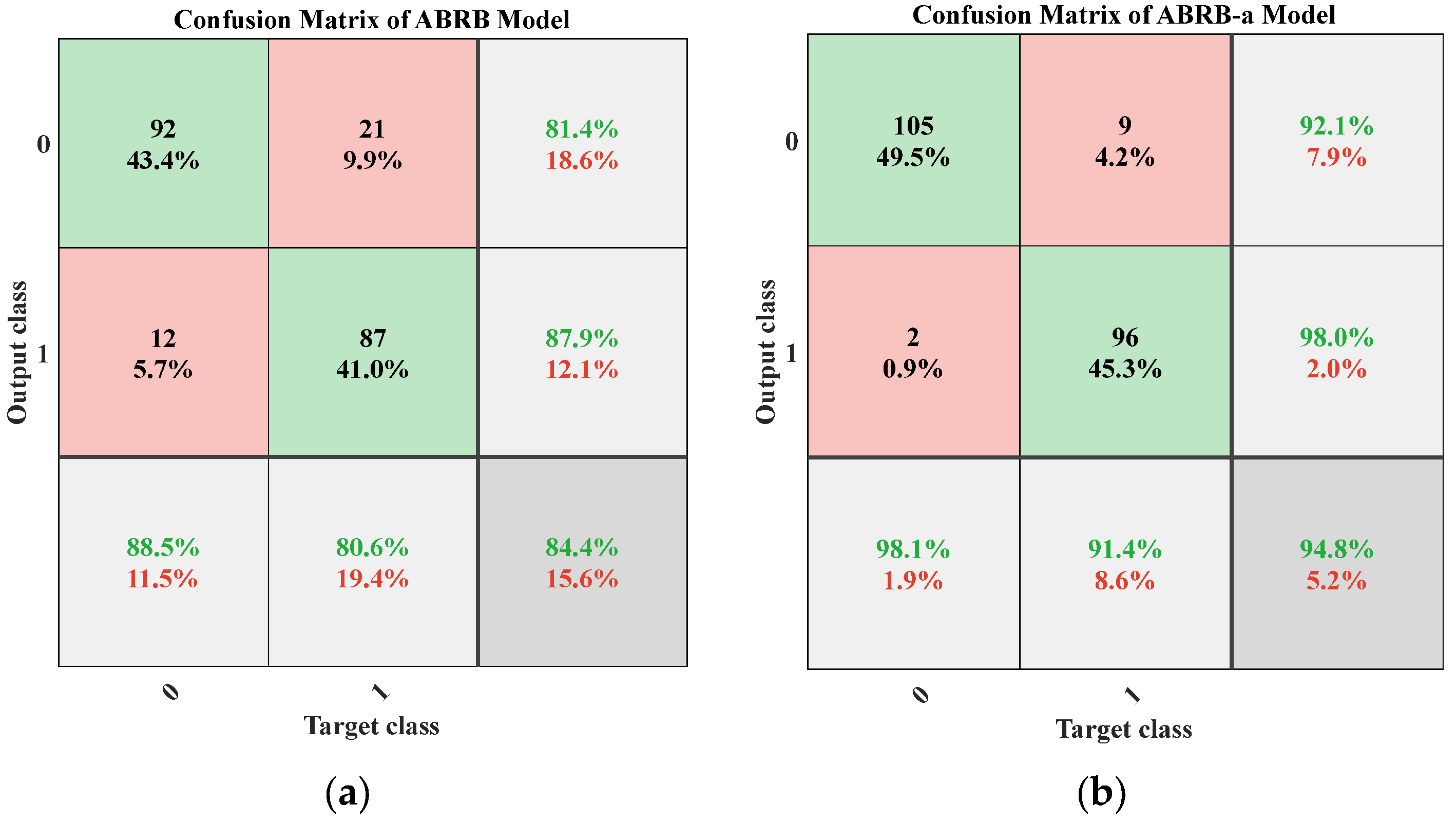
Experimental analysis was conducted in this study based on the prediction model constructed in Section 4.2. Experimental results show this. After optimization, the model performance has been significantly improved. As shown in Figure 8. Figure 8a,b are the confusion matrices of ABRB and ABRB-a, respectively. It can be clearly seen that the number of misclassified samples for Label 0 has been reduced from 21 in Figure 8a to 9 in Figure 8b. Meanwhile, the number of misclassified samples for Label 1 has also been reduced from 12 to 2.
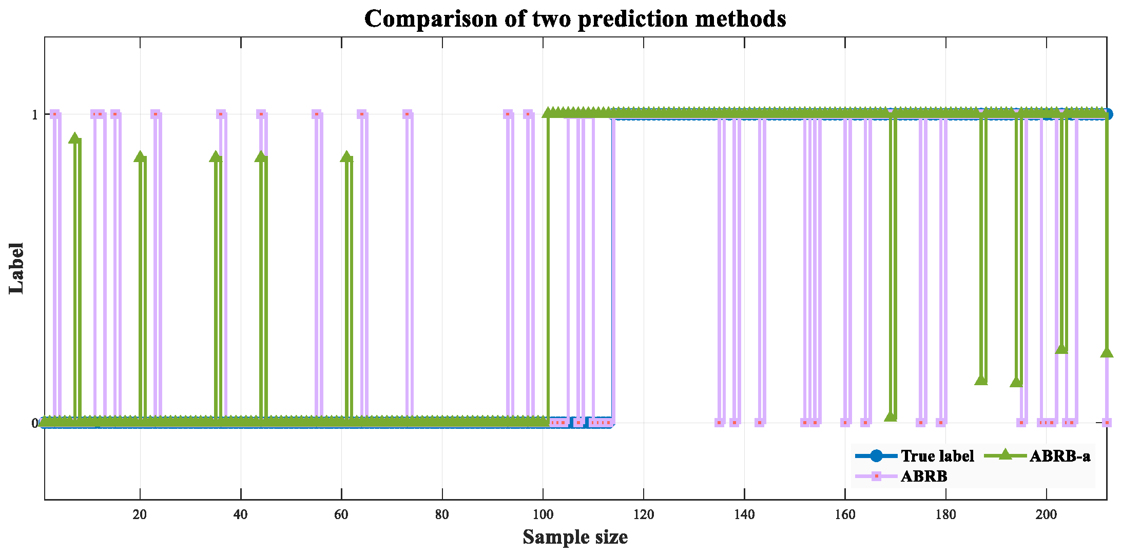
As shown in Figure 9, compared with the ABRB model, the ABRB-a model demonstrates significant performance improvement in both category 0 and category 1.
Based on the initial parameter settings (as shown in Table 4), the parameters were adjusted through an optimization algorithm, resulting in the optimized results as shown in Table 5. The optimization process updated the attribute weights, rule weights, and belief degree, making them more in line with the distribution characteristics of the actual data.
The belief rule base (BRB) inherently possesses good interpretability, mainly due to its rule structure in the form of IF-THEN statements, which makes the reasoning process clear and visible. As shown in Table 4 and Table 5, these tables compare the initial model with the optimized model parameters, allowing for a clear view of changes in attribute weights, rule weights, and output belief levels. This visual representation not only enhances the understandability of the model but also provides an intuitive basis for analyzing the impact of parameter adjustments during optimization.

4.4. Comparative Experiment

To verify the stability performance of the ABRB-a model, this section conducts a systematic comparative analysis with six benchmark models. Section 4.4.1 determines the calculation formulas for the five core evaluation indicators. Section 4.4.2, on the basis of these core indicators, conducts an in-depth analysis of the diagnostic performance differences among the models. Finally, Section 4.4.3 comprehensively presents the significant advantages of the ABRB-a model over other comparison models through multi-dimensional comparative experiments, from quantitative indicators to qualitative analysis.

4.4.1. Core Evaluation Criteria

The evaluation indicators serve as the key basis for measuring the robustness of a model. In this study, six core evaluation indicators, including the accuracy, precision, recall, and F1 score, are selected to conduct a comprehensive assessment of the performance of the ABRB-a model. The calculation formulas for each indicator are as follows:
A c c u r a c y = C N u m T N u m × 100
R e c a l l = T P T P + F N
P r e c i s i o n = T P T P + F P
F 1 = 2 × ( P r e c i s i o n × R e c a l l ) P r e c i s i o n + R e c a l l
M S E = 1 γ i = 1 γ η i η ^ i 2
where A c c u r a c y represents the overall accuracy of the model, C N u m represents the number of samples that produce correct output results, and T N u m represents the total number of evaluated samples. TP (true positive) indicates the number of true positive cases successfully identified by the model, whereas FN (false negative) indicates the number of true positive cases that the model failed to identify. The F1 score ranges from 0 to 1, with values close to 1 indicating better fault diagnosis in balancing precision and recall. γ is the number of samples, η i is the true value, and η ^ i is the predicted value.

4.4.2. Model Prediction Performance Analysis

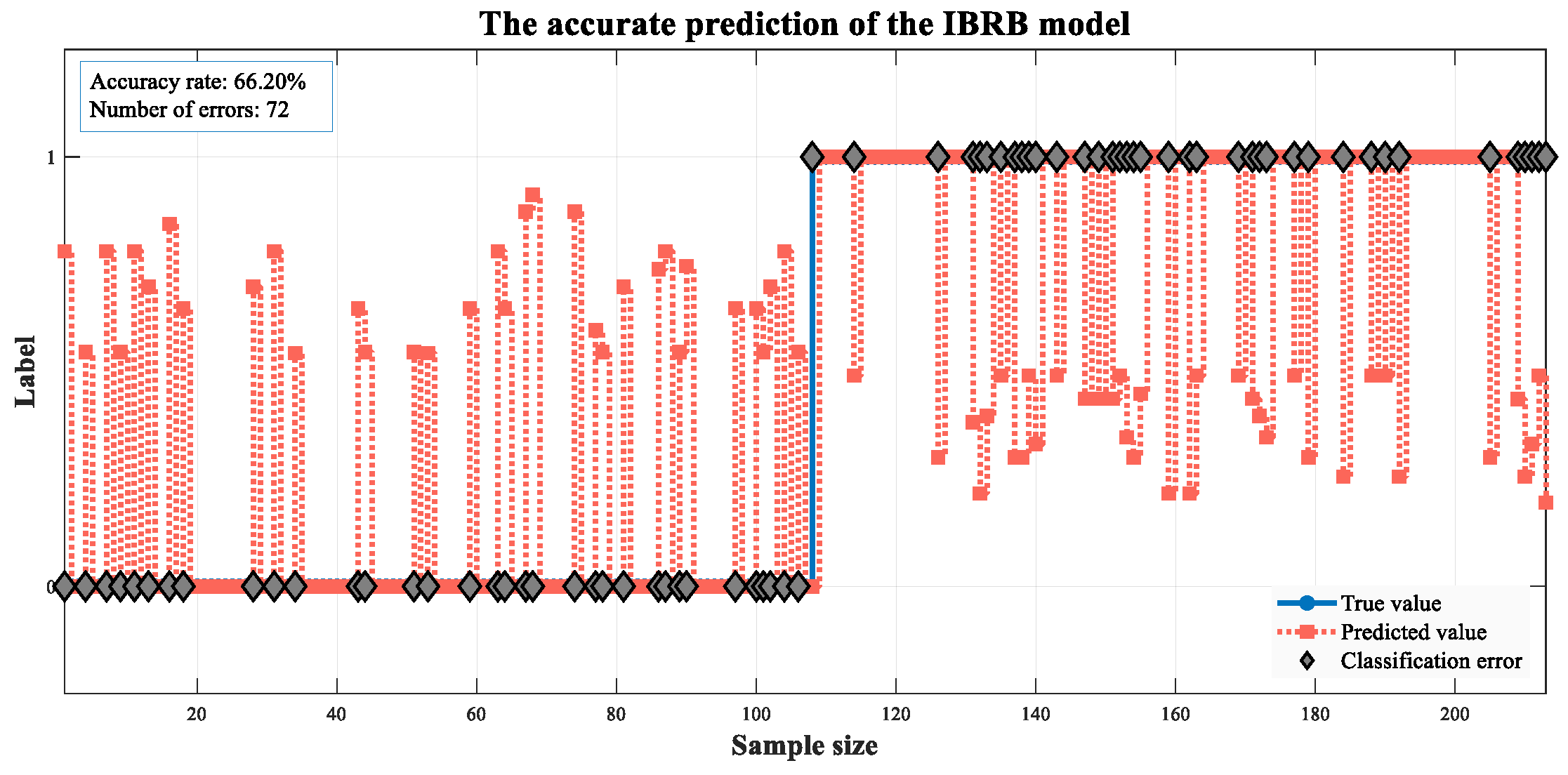
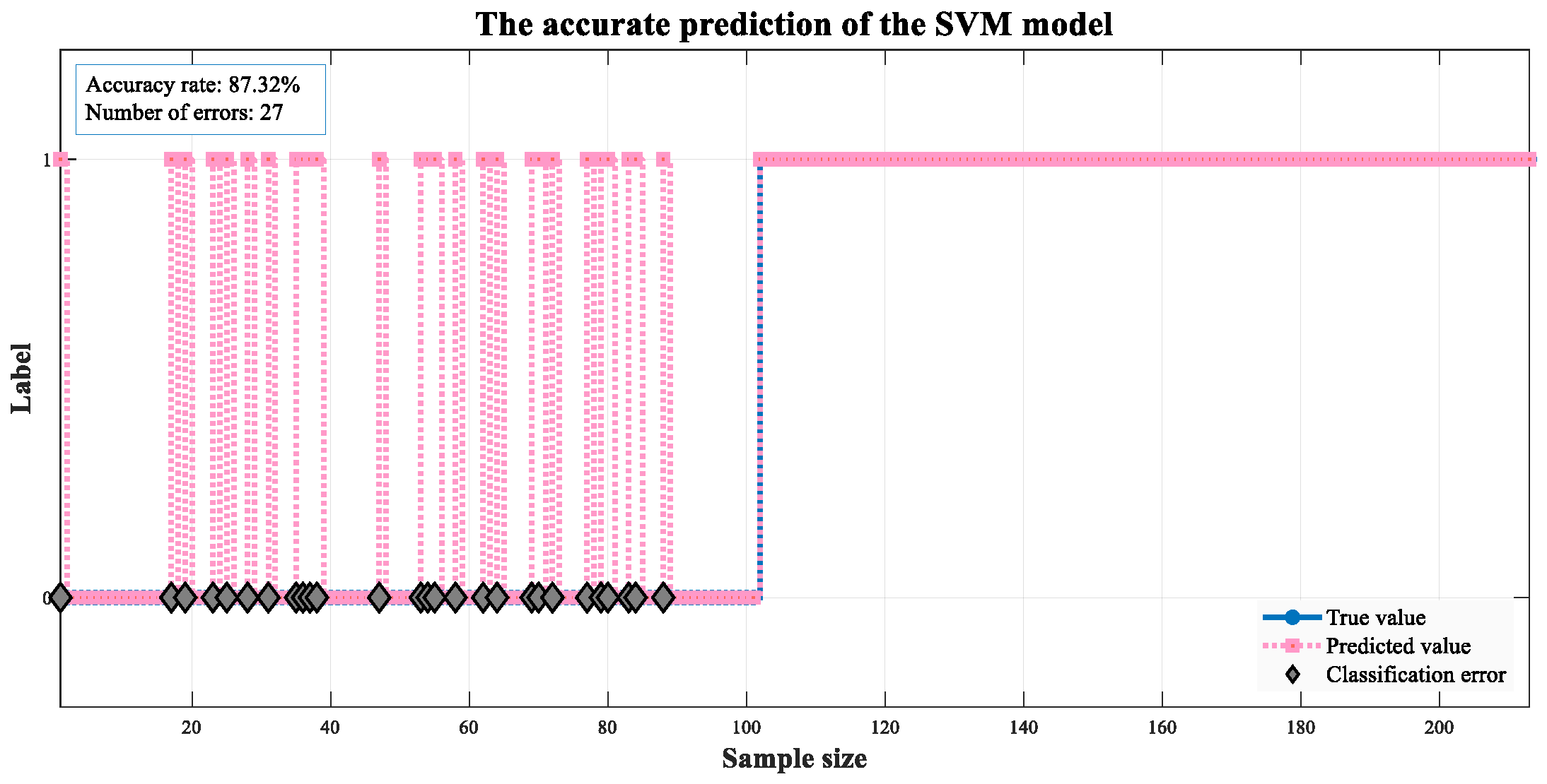
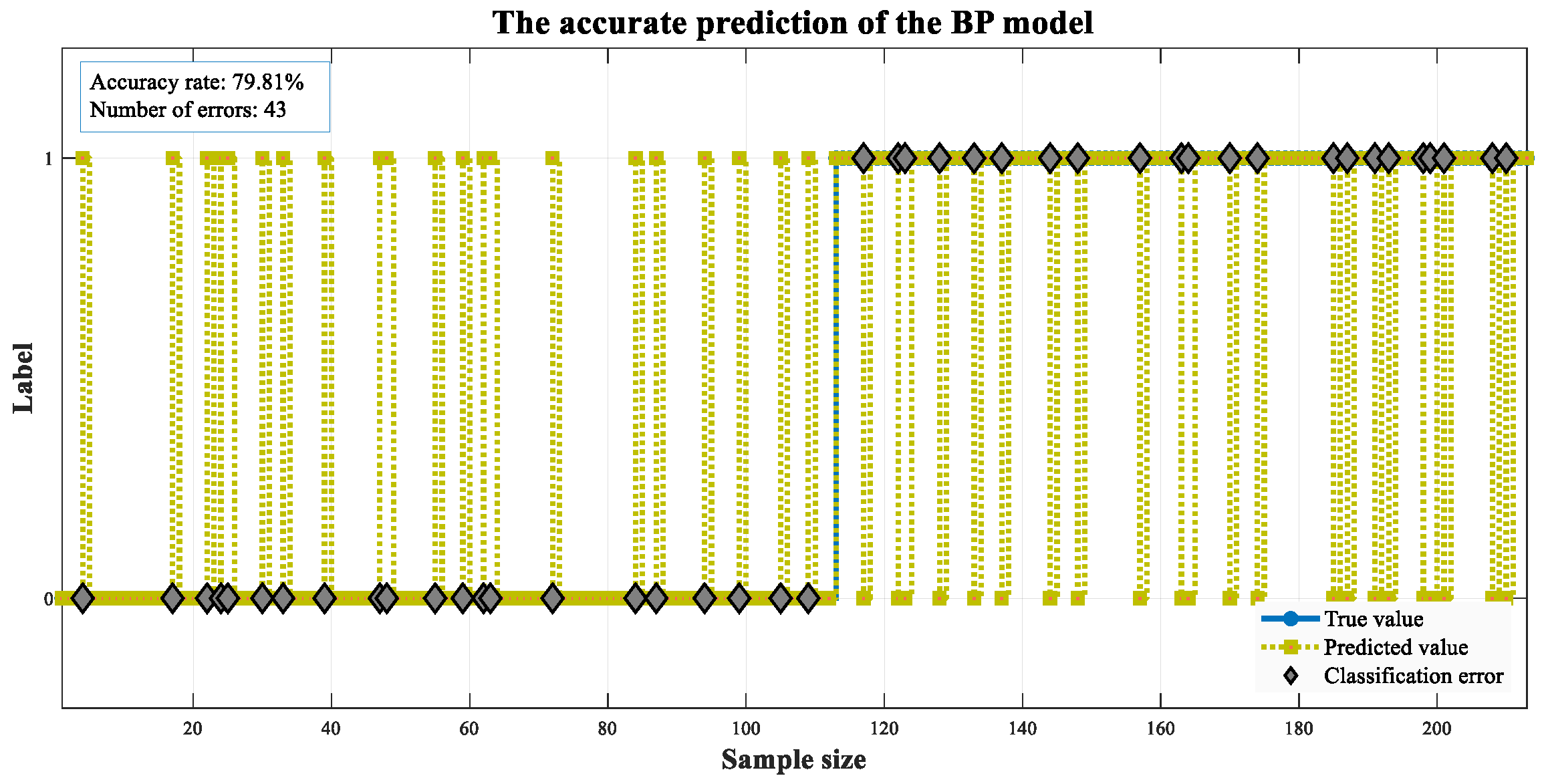
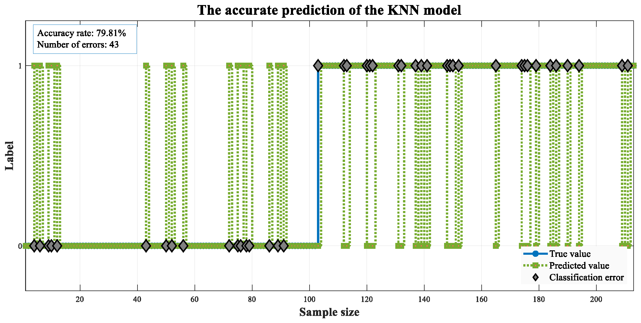
To evaluate the prediction performance of the ABRB-a model, this subsection assesses the performance of the ABRB-a model against typical black-box models (ABRB, EBRB, IBRB) and white-box models (SVM, BP, KNN) in the classification task. The parameter settings for each model are shown in Table 6. All models have been fully tuned to ensure fairness in comparison.
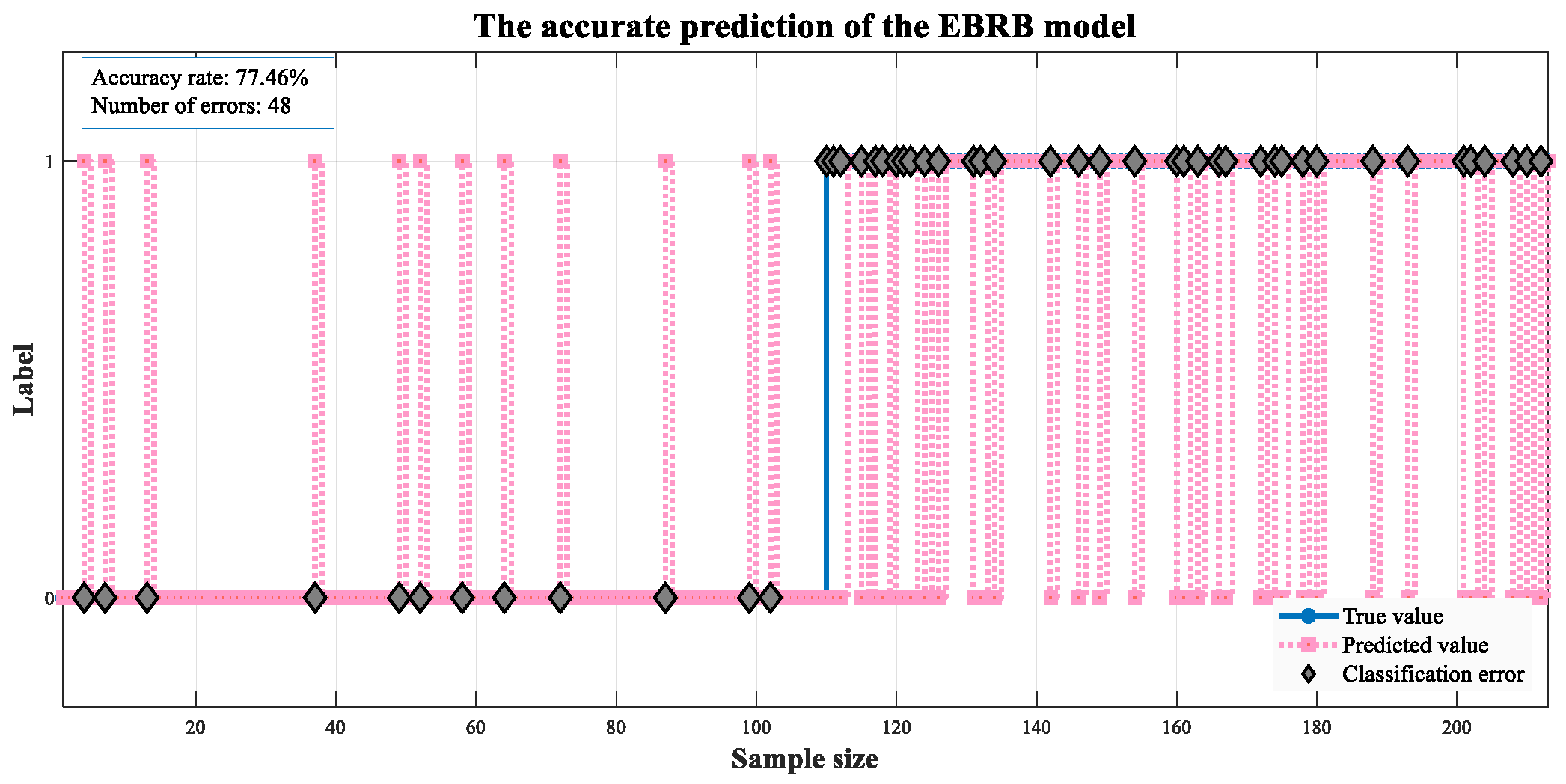
By comparing the models based on the parameters listed in Table 6, the analysis results show that the ABRB-a model has a significant advantage in overall diagnostic accuracy. As shown in Figure 9, compared with ABRB, ABRB-a exhibits excellent performance in all categories; while the other models shown in Figure 10, Figure 11, Figure 12, Figure 13 and Figure 14 perform relatively poorly in both category 0 and category 1. In contrast, the ABRB-a model demonstrates stable and outstanding classification performance in all test categories. This result preliminarily verifies that the ABRB-a model has strong generalization ability and can effectively adapt to the diagnostic requirements of different categories, demonstrating good practical potential.

4.4.3. Multi-Dimensional Comparison Verification

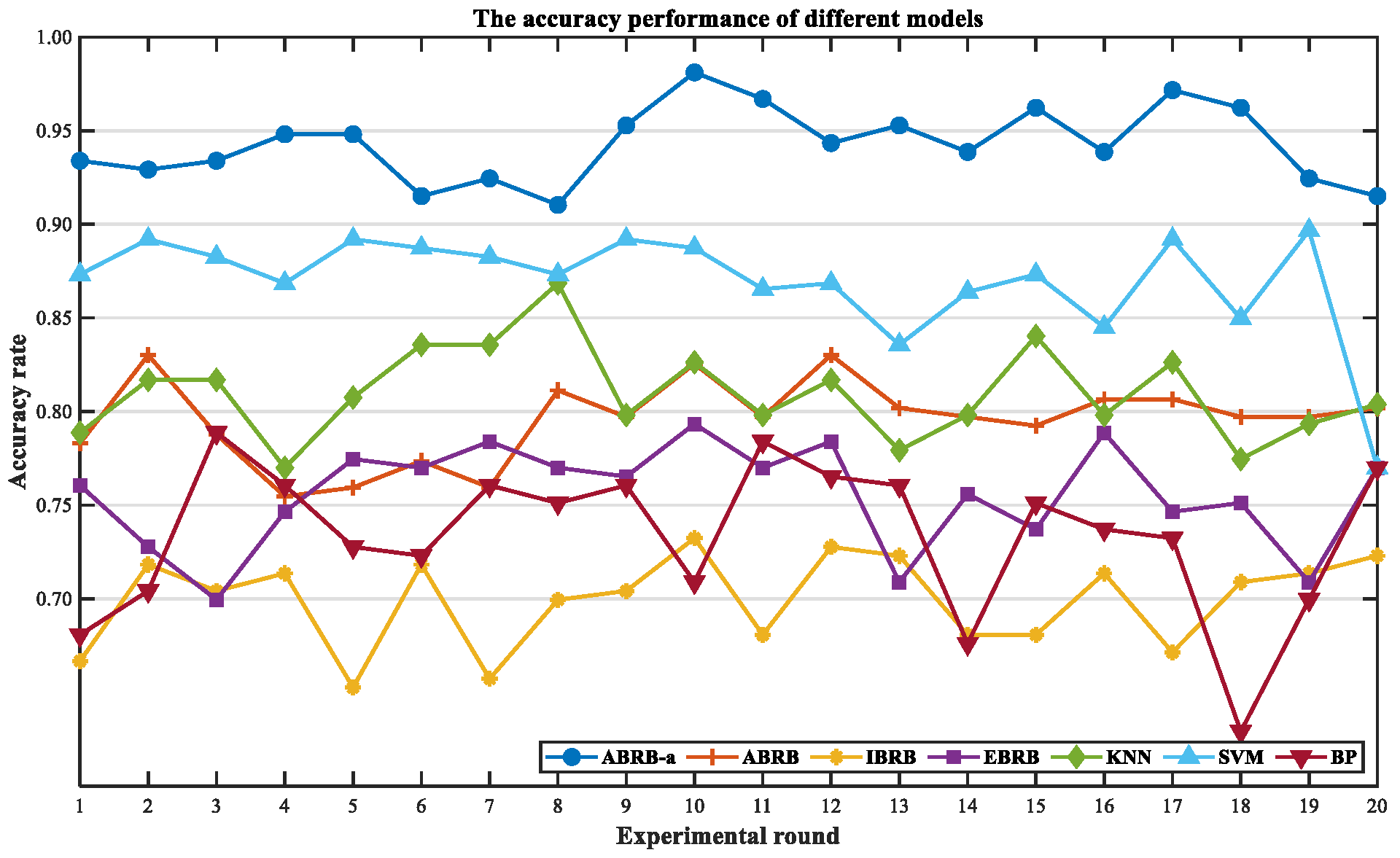
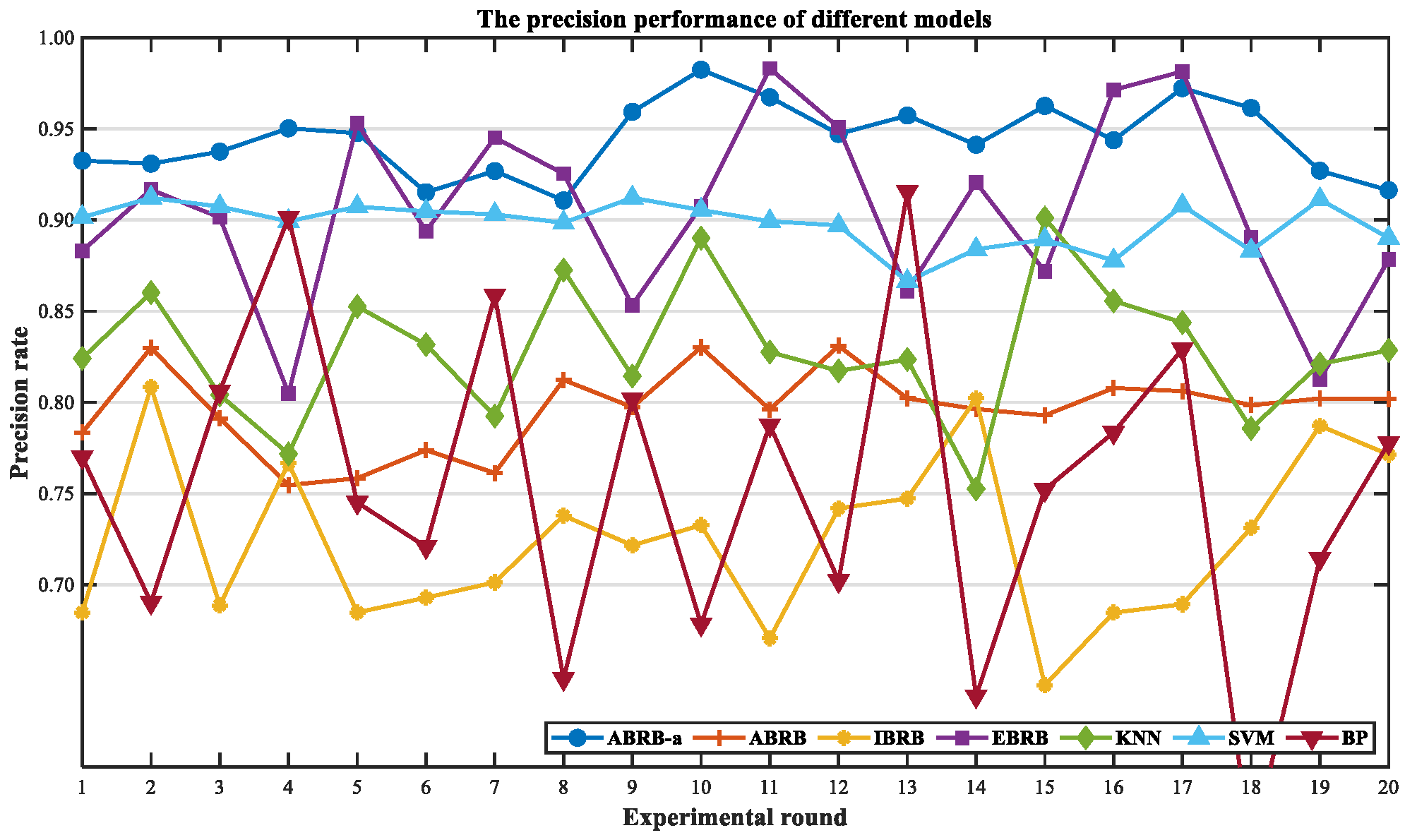
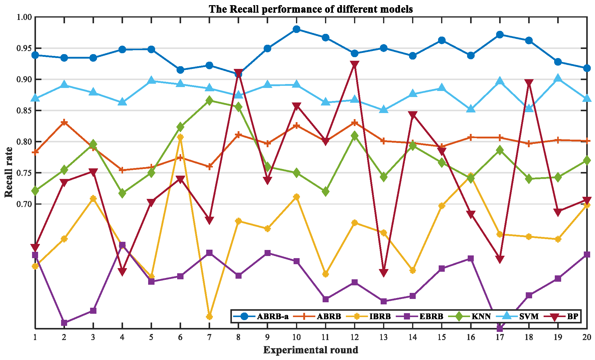
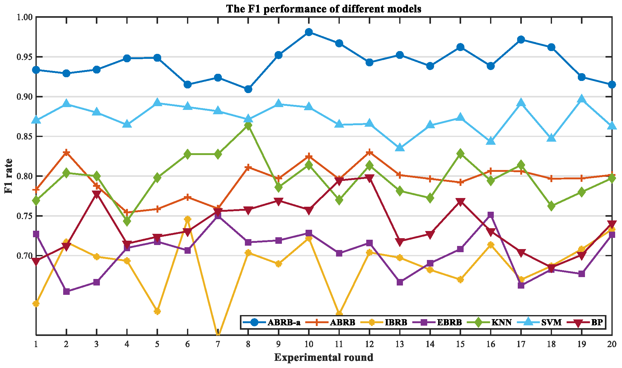
In this section, to further verify the stability of the ABRB-a model, we conducted twenty independent repeated experiments on all the comparison models to ensure the reliability and reproducibility of the experimental results. The dynamic change trend of the experimental results is shown in Figure 15, Figure 16, Figure 17 and Figure 18, where the horizontal axis represents the experimental rounds and the vertical axis reflects the model performance indicators. Through visual analysis, it can be clearly observed that in all the experimental rounds, the performance curve of the ABRB-a model not only consistently outperforms the other comparison models but also shows smaller performance fluctuations. This preliminary verification demonstrates that the model has significant performance advantages and stability.
The dataset was divided into different proportions, and twenty independent repeated experiments were conducted for each proportion. The average calculation results of the performance indicators of each model under different data proportions are shown in Table 7, Table 8 and Table 9. The experimental data indicate that the ABRB-a model has significant advantages in all evaluation indicators. Compared with other BRB models, the accuracy, precision, recall rate and F1 score of this model are significantly better than those of other models. In the comparison of black-box models, its performance advantage has also achieved remarkable results. These experimental results fully confirm the stability and superiority of the ABRB-a model.
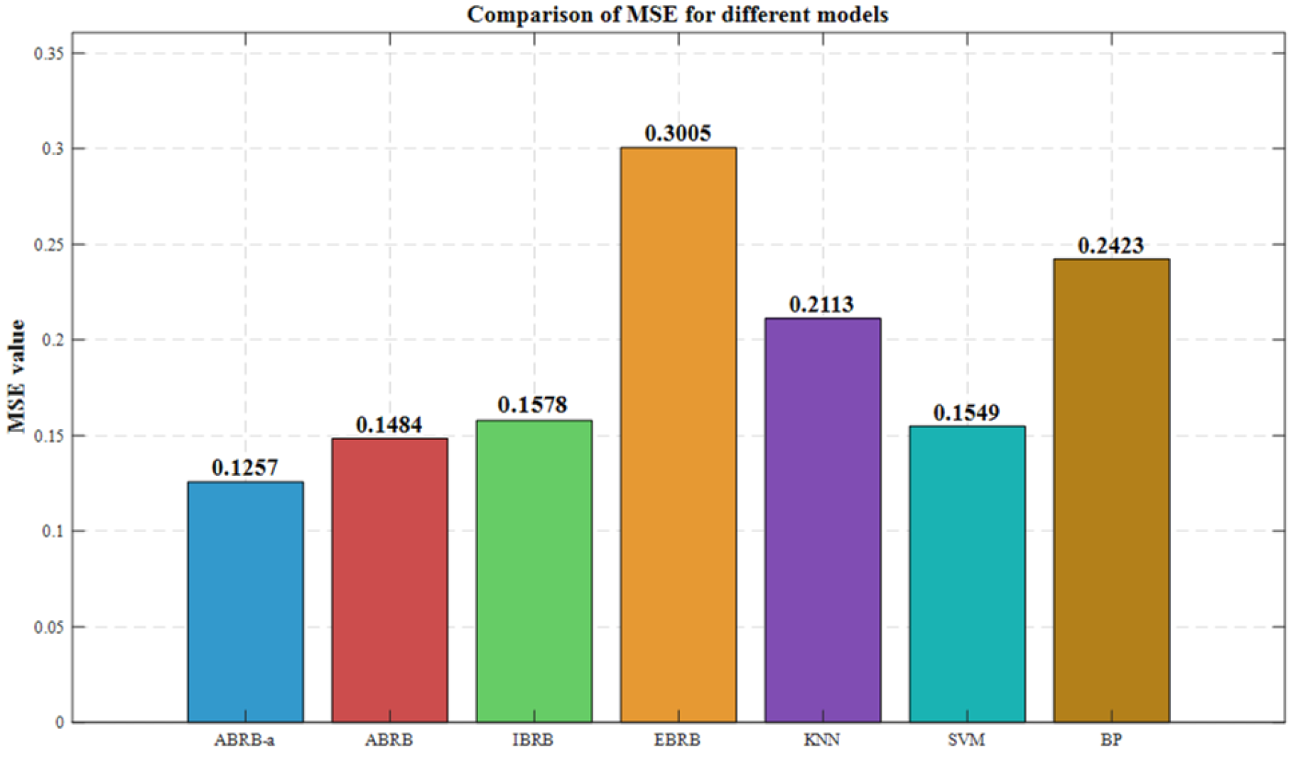
In order to conduct a comprehensive evaluation of the performance of the ABRB-a model, this study employed the MSE key metric for quantitative analysis. As shown in the experimental results depicted in Figure 19, the ABRB-a model demonstrated an advantage in this metric. This performance improvement fully substantiates the superiority of the ABRB-a model in terms of prediction accuracy and stability, indicating that it possesses higher accuracy when handling related tasks.
To verify the rationality of using Mahalanobis distance as a constraint, this study compared it with Euclidean distance. As shown in Table 10, in terms of the key indicator of mean squared error (MSE), Mahalanobis distance outperformed Euclidean distance, with a lower MSE value. Moreover, when measuring the distance between samples and the center of the population, Mahalanobis distance can comprehensively consider the covariance structure among various features, effectively eliminating the influence of differences in dimensions and variable scales. Since this study involves multi-dimensional attribute variables, Mahalanobis distance has obvious advantages in such scenarios, while simple measurement methods like Euclidean distance are difficult to fully reflect the complex correlations among variables.
To assess the robustness of the ABRB-a model, systematic perturbation tests were conducted on the key parameters in the experimental part. As shown in Table 11, when the control factors fluctuated within the preset range, the key performance indicators of the model only showed minor changes, and no significant degradation in performance occurred. This result fully proves that the ABRB-a model has excellent stability when facing parameter perturbations, and its output results are reliable.

4.5. Generalization Verification

To verify the generalization ability of the ABRB-a model, this paper conducted experiments based on the publicly available student academic performance dataset on the Kaggle platform (https://www.kaggle.com/datasets/rabieelkharoua/students-performance-dataset (accessed on: 30 September 2025)). This dataset has obtained usage permission (licensing link: https://creativecommons.org/licenses/by/4.0/ (accessed on: 30 September 2025)), and all data have been anonymized, not involving any personal privacy information, and can be safely used for academic research. The dataset contains 12 attributes and 1 result label. After feature selection, this paper selected Absences, Parental Support, Study Time Weekly, Tutoring, and Extracurricular as the model inputs, and used Grade Class as the prediction label.
The processed dataset was divided into a training set and a test set in a ratio of 7:3, and repeated experiments were conducted. The final results are presented in Table 12. It can be clearly seen from the table that the ABRB-a model demonstrates significant advantages in multiple indicators, and its performance is significantly better than the comparison methods, thereby fully verifying that this model has strong generalization ability.

4.6. Experimental Summary

Through experimental analysis, this study systematically compared the ABRB-a model with several other benchmark models across multiple dimensions and evaluation indicators. At the same time, generalization ability was verified on different datasets. The experimental results show that the effectiveness of the ABRB-a model in complex educational systems has been fully validated. This model can help teachers accurately identify the key factors affecting student performance, thereby optimizing teaching strategies, improving teaching effectiveness, and providing reliable data support for educational decision-making. The comparative experiments further confirmed the important application value and broad development prospects of the ABRB-a model in the field of education. The outstanding performance of the ABRB-a model is mainly reflected in the following three aspects:
(1) Optimization of reference point selection: Traditional models usually rely on expert experience or historical data to determine reference points and lack interpretability. This study adopted the agglomerative hierarchical clustering algorithm for reference point selection, significantly improving the accuracy and interpretability of the model and providing a more reliable basis for teachers to analyze students’ performance.
(2) Introduction of the Mahalanobis distance constraint: During the algorithm optimization process, the Mahalanobis distance constraint mechanism was introduced, effectively improving the accuracy of model parameter estimation and thereby enhancing the overall prediction accuracy.
(3) Readability of rules: The ABRB-a model uses IF-THEN form rules for representation, which have good readability. This intuitive rule expression method helps teachers understand the student characteristics corresponding to each rule, thereby enabling them to comprehensively understand students’ learning status and formulate personalized teaching plans.

5. Conclusions

This study proposes an approximate belief rule base (ABRB-a) student examination passing prediction method based on adaptive reference point selection using symmetry. This method achieves efficient prediction through the following innovations. First, a hierarchical agglomerative clustering algorithm is used to adaptively obtain reference points, overcoming the subjectivity and limitations of traditional methods that rely on expert experience and significantly enhancing the stability of the model. Second, an optimized P-CMA-ES-M algorithm with Mahalanobis distance constraints is introduced to optimize the model parameters, further enhancing the prediction accuracy and robustness of the model. The experimental results show that the ABRB-a model performs excellently in terms of stability and generalizability.
The ABRB-a model enables teachers to identify key influencing factors through intuitive rule interpretation and formulate targeted teaching strategies. Although the model performs poorly in handling cases of exam failure caused by emotional factors, it will be continuously improved in the future by integrating psychological characteristic indicators, specifically by collecting students’ accessible physiological signals and recording observable emotional behaviors to turn abstract emotions into quantifiable features that fit the ABRB-a mode’s attribute input requirements, optimizing parameter learning algorithms and expanding application scenarios to further enhance the adaptability and generalizability ability of the model. Finally, the current hierarchical clustering-based methods have laid the foundation for handling more complex symmetrical forms. Therefore, this has also become one of the core research directions in the future, namely exploring how to expand this framework to identify and model more complex asymmetric patterns in the data.

6. The Meaning of the Letters

The specific meanings of all the letters are fully explained in the appendix of the article. For detailed explanations, please refer to Appendix A.

Author Contributions

Conceptualization, J.L. and H.Z.; methodology, J.L.; software, K.L.; validation, K.L., H.Z. and J.H.; formal analysis, J.H.; investigation, J.L.; data curation, C.Y.; writing—original draft preparation, J.L.; writing—review and editing, J.L., K.L. and C.Y.; All authors have read and agreed to the published version of the manuscript.

Funding

This work was supported in part by Key Laboratory of Equipment Data Security and Guarantee Technology, Ministry of Education under Grant No. GDZB2024050100, in part by the Natural Science Foundation of Heilongjiang Province under Grant No. PL2024G009, in part by the Basic Research Support Program for Outstanding Young Teachers in Provincial Undergraduate Universities of Heilongjiang Province under Grant No. YQJH2024116.

Data Availability Statement

The data used in this article is sourced from Kaggle. Please visit the following website to obtain: https://www.kaggle.com/datasets/amrmaree/student-performance-prediction (accessed on: 30 September 2025). Generalization experiment dataset: https://www.kaggle.com/datasets/rabieelkharoua/students-performance-dataset (accessed on: 30 September 2025).

Conflicts of Interest

The authors declare no conflicts of interest.

Appendix A

All variables are defined in Table A1.
Table A1. Dictionary of notations.
NONotationMeaning
1 Q The initial parameters of the model
2 F ( · ) The data mining process
3 α The educational data
4 φ The Data Mining Parameters
5 Q b e s t The optimization parameters of the model
6 G ( · ) The model optimization process
7 L The parameters of P-CMA-ES-M
8 y The prediction result of the model
9 X ˜ The input feature set
10 M The total number of input attributes
11 H i The total number of the rules
11 y = ( · ) The nonlinear functional relationship between the system characteristics and the predicted value
12 R i , h The h t h belief rule
13 A ^ i , h The h t h reference value of X ˜ i
14 β n , i , h The belief degree of D N
15 D N The n t h result belief degree
16 θ i , h The rule weight of R i , h
17 δ i The attribute weight of the premise
18 Φ N × M type matrix
19 N The quantity of the dataset
20 ς A data vector representing the observed values of all samples for the i t h feature
21 ς a , ς b The specific sample observation values at the a t h and b t h positions within vector ς
22 C i , C l The i t h cluster and the l t h
23 Γ The number of clusters
24 μ ¯ C i The arithmetic mean of the i t h sample value within the cluster
25 Δ ( C i , C l ) The sum of squared within-cluster variances caused by merging clusters C i and C l
26 μ Γ The center of the Γ t h cluster
27 v combined A comprehensive vector consisting of the global minimum value
28 The difference vector
29 ν The most symmetrical set of reference values
30 Δ A constant value between two adjacent reference values
31 δ i The normalization weight of the attributes
32 a i h The matching degree of the h t h rule
33 L The number of all rules
34 w i , h The rule activation weights
35 γ n i , h An intermediate variable
36 S The set of belief distributions
37 A The input vector of the actual system
38 μ ( · ) The utility function
39 M S E ( · ) The prediction accuracy of the model
40 g The current number of iterations
41 C The covariance matrix
42 ε The population size
43 k The offspring population size
44 λ The initial step size
45 m e a n ( g ) The mean of the optimal whole in the g t h generation
46 ψ The parameter set
47 Ω k g + 1 The population generated in the ( g + 1 ) t h generation
48 N · A normal distribution
49 D M The mahalanobis distance
50 d The distance range
51 β n , i , h g + 1 The ( g + 1 ) t h generation of reasonable belief distribution
52 A e The parameter vector
53 n e The number of parameters
54 j The number of equation constraints contained in the constraints
55 ω k The weighting factor
56 τ An intermediate variable
57 c The learning rate
58 p c The evolution path of the covariance matrix path
59 C c The backward time horizon of the evolution path
60 d σ The damping coefficient
61 G N 0 , Ι The expected value of the Euclidean norm N 0 , Ι
62 Ι The identity matrix
63 c σ The parameters of the conjugate evolution path p c
64 C N u m The number of samples that produce correct output results
65 T N u m The total number of evaluated samples
66 T P The true positive
67 F N The false negative
68 γ The number of samples
69 η i The true value
70 η ^ i The predicted value

References

  1. Al-Shehri, H.; Al-Qarni, A.; Al-Saati, L.; Batoaq, A.; Badukhen, H.; Alrashed, S.; Alhiyafi, J.; Olatunji, S.O. Student performance prediction using support vector machine and k-nearest neighbor. In Proceedings of the 2017 IEEE 30th Canadian Conference on Electrical and Computer Engineering (CCECE), Windsor, ON, Canada, 30 April–3 May 2017; IEEE: Piscataway, NJ, USA, 2017; pp. 1–4. [Google Scholar]
  2. Kabakchieva, D. Student performance prediction by using data mining classification algorithms. Int. J. Comput. Sci. Manag. Res. 2012, 1, 686–690. [Google Scholar]
  3. Raftopoulos, G.; Davrazos, G.; Kotsiantis, S. Fair and Transparent Student Admission Prediction Using Machine Learning Models. Algorithms 2024, 17, 572. [Google Scholar] [CrossRef]
  4. Thuy, N.T.; Ha, N.T.; Trung, N.N.; Binh, V.T.; Hang, N.T.; Binh, V.T. Comparing the Effectiveness of Machine Learning and Deep Learning Models in Student Credit Scoring: A Case Study in Vietnam. Risks 2025, 13, 99. [Google Scholar] [CrossRef]
  5. Koukaras, C.; Hatzikraniotis, E.; Mitsiaki, M.; Koukaras, P.; Tjortjis, C.; Stavrinides, S.G. Revolutionising Educational Management with AI and Wireless Networks: A Framework for Smart Resource Allocation and Decision-Making. Appl. Sci. 2025, 15, 293. [Google Scholar] [CrossRef]
  6. Kim, B.H.; Vizitei, E.; Ganapathi, V. GritNet: Student performance prediction with deep learning. arXiv 2018, arXiv:1804.07405. [Google Scholar] [CrossRef]
  7. Connor, C.M. Using technology and assessment to personalize instruction: Preventing reading problems. Prev. Sci. 2019, 20, 89–99. [Google Scholar] [CrossRef]
  8. Grayson, A.; Miller, H.; Clarke, D.D. Identifying barriers to help-seeking: A qualitative analysis of students’ preparedness to seek help from tutors. Br. J. Guid. Couns. 1998, 26, 237–253. [Google Scholar] [CrossRef]
  9. Yue, L.; Hu, P.; Chu, S.-C.; Pan, J.-S. Multi-objective gray wolf optimizer with cost-sensitive feature selection for Predicting students’ Academic performance in college english. Mathematics 2023, 11, 3396. [Google Scholar] [CrossRef]
  10. Almalawi, A.; Soh, B.; Li, A.; Samra, H. Predictive Models for Educational Purposes: A Systematic Review. Big Data Cogn. Comput. 2024, 8, 187. [Google Scholar] [CrossRef]
  11. Cao, W.; Mai, N.T.; Liu, W. Adaptive Knowledge Assessment via Symmetric Hierarchical Bayesian Neural Networks with Graph Symmetry-Aware Concept Dependencies. Symmetry 2025, 17, 1332. [Google Scholar] [CrossRef]
  12. Triveni, G.R.; Danish, F.; Albalawi, O. Advancing Survey Sampling Efficiency under Stratified Random Sampling and Post-Stratification: Leveraging Symmetry for Enhanced Estimation Accuracy in the Prediction of Exam Scores. Symmetry 2024, 16, 604. [Google Scholar] [CrossRef]
  13. Wang, S.; Luo, B. Academic achievement prediction in higher education through interpretable modeling. PLoS ONE 2024, 19, e0309838. [Google Scholar] [CrossRef] [PubMed]
  14. Abromavičius, V.; Serackis, A.; Katkevičius, A.; Kazlauskas, M.; Sledevič, T. Prediction of exam scores using a multi-sensor approach for wearable exam stress dataset with uniform preprocessing. Technol. Health Care 2023, 31, 2499–2511. [Google Scholar] [CrossRef] [PubMed]
  15. Khairy, D.; Alharbi, N.; Amasha, M.A.; Areed, M.F.; Alkhalaf, S.; Abougalala, R.A. Prediction of student exam performance using data mining classification algorithms. Educ. Inf. Technol. 2024, 29, 21621–21645. [Google Scholar] [CrossRef]
  16. Isinkaye, F.O.; Folajimi, Y.O.; Ojokoh, B.A. Recommendation systems: Principles, methods and evaluation. Egypt. Inform. J. 2015, 16, 261–273. [Google Scholar] [CrossRef]
  17. Lü, L.; Medo, M.; Yeung, C.H.; Zhang, Y.-C.; Zhang, Z.-K.; Zhou, T. Recommender systems. Phys. Rep. 2012, 519, 1–49. [Google Scholar] [CrossRef]
  18. Saganowski, S. Bringing emotion recognition out of the lab into real life: Recent advances in sensors and machine learning. Electronics 2022, 11, 496. [Google Scholar] [CrossRef]
  19. Yang, J.-B.; Liu, J.; Wang, J.; Sii, H.-S.; Wang, H.-W. Belief rule-base inference methodology using the evidential reasoning approach-RIMER. IEEE Trans. Syst. Man Cybern.—Part A Syst. Hum. 2006, 36, 266–285. [Google Scholar] [CrossRef]
  20. Chen, M.; Zhou, Z.; Han, X.; Feng, Z. A Text-Oriented Fault Diagnosis Method for Electromechanical Device Based on Belief Rule Base. Mathematics 2023, 11, 1814. [Google Scholar] [CrossRef]
  21. Cheng, X.; Qian, G.; He, W.; Zhou, G. A liquid launch vehicle safety assessment model based on semi-quantitative interval belief rule base. Mathematics 2022, 10, 4772. [Google Scholar] [CrossRef]
  22. Chen, H.; Zhou, G.; Zhang, X.; Zhu, H.; He, W. Learning Emotion assessment method based on belief rule base and evidential reasoning. Mathematics 2023, 11, 1152. [Google Scholar] [CrossRef]
  23. Levin, M.S. Modular System Design and Evaluation; Springer: Cham, Switzerland, 2015. [Google Scholar]
  24. Gligorea, I.; Yaseen, M.U.; Cioca, M.; Gorski, H.; Oancea, R. An interpretable framework for an efficient analysis of students’ academic performance. Sustainability 2022, 14, 8885. [Google Scholar] [CrossRef]
  25. Mascharka, D.; Tran, P.; Soklaski, R.; Majumdar, A. Transparency by design: Closing the gap between performance and interpretability in visual reasoning. In Proceedings of the IEEE Conference on Computer Vision and Pattern Recognition, Salt Lake City, UT, USA, 18–23 June 2018; pp. 4942–4950. [Google Scholar]
  26. Sun, C.; Yang, R.; He, W.; Zhu, H.J. A novel belief rule base expert system with interval-valued references. Sci. Rep. 2022, 12, 6786. [Google Scholar] [CrossRef] [PubMed]
  27. Ran, X.; Xi, Y.; Lu, Y.; Wang, X.; Lu, Z.J. Comprehensive survey on hierarchical clustering algorithms and the recent developments. Artif. Intell. Rev. 2023, 56, 8219–8264. [Google Scholar] [CrossRef]
  28. Murtagh, F.; Contreras, P.J. Algorithms for hierarchical clustering: An overview, II. Wiley Interdiscip. Rev. Data Min. Knowl. Discov. 2017, 7, e1219. [Google Scholar] [CrossRef]
  29. Dhillon, I.S.; Mallela, S.; Kumar, R. Enhanced word clustering for hierarchical text classification. In Proceedings of the Eighth ACM SIGKDD International Conference on Knowledge Discovery and Data Mining, Edmonton, AB, Canada, 23–26 June 2002; pp. 191–200. [Google Scholar]
  30. Sahoo, N.; Callan, J.; Krishnan, R.; Duncan, G.; Padman, R. Incremental hierarchical clustering of text documents. In Proceedings of the 15th ACM International Conference on Information and Knowledge Management, Arlington, VA, USA, 6 November 2006; pp. 357–366. [Google Scholar]
  31. Dasgupta, S.; Long, P.M. Performance guarantees for hierarchical clustering. J. Comput. Syst. Sci. 2005, 70, 555–569. [Google Scholar] [CrossRef]
  32. Mittal, H.; Pandey, A.C.; Saraswat, M.; Kumar, S.; Pal, R.; Modwel, G. A comprehensive survey of image segmentation: Clustering methods, performance parameters, and benchmark datasets. Multimed. Tools Appl. 2022, 81, 35001–35026. [Google Scholar] [CrossRef]
  33. Wang, Y.-M.; Yang, L.-H.; Fu, Y.-G.; Chang, L.-L.; Chin, K.-S. Dynamic rule adjustment approach for optimizing belief rule-base expert system. Knowl.-Based Syst. 2016, 96, 40–60. [Google Scholar] [CrossRef]
  34. Xu, D.-L.; Liu, J.; Yang, J.-B.; Liu, G.-P.; Wang, J.; Jenkinson, I.; Ren, J. Inference and learning methodology of belief-rule-based expert system for pipeline leak detection. Expert Syst. Appl. 2007, 32, 103–113. [Google Scholar] [CrossRef]
  35. Chang, L.; Xu, X.; Liu, Z.-g.; Qian, B.; Xu, X.; Chen, Y.-W. BRB prediction with customized attributes weights and tradeoff analysis for concurrent fault diagnosis. IEEE Syst. J. 2020, 15, 1179–1190. [Google Scholar] [CrossRef]
  36. Cao, Y.; Zhou, Z.; Hu, C.; He, W.; Tang, S. On the interpretability of belief rule-based expert systems. IEEE Trans. Fuzzy Syst. 2020, 29, 3489–3503. [Google Scholar] [CrossRef]
  37. Zhang, Z.; He, W.; Zhou, G.; Li, H.; Cao, Y. A new interpretable behavior prediction method based on belief rule base with rule reliability measurement. Reliab. Eng. Syst. Saf. 2025, 256, 110712. [Google Scholar] [CrossRef]
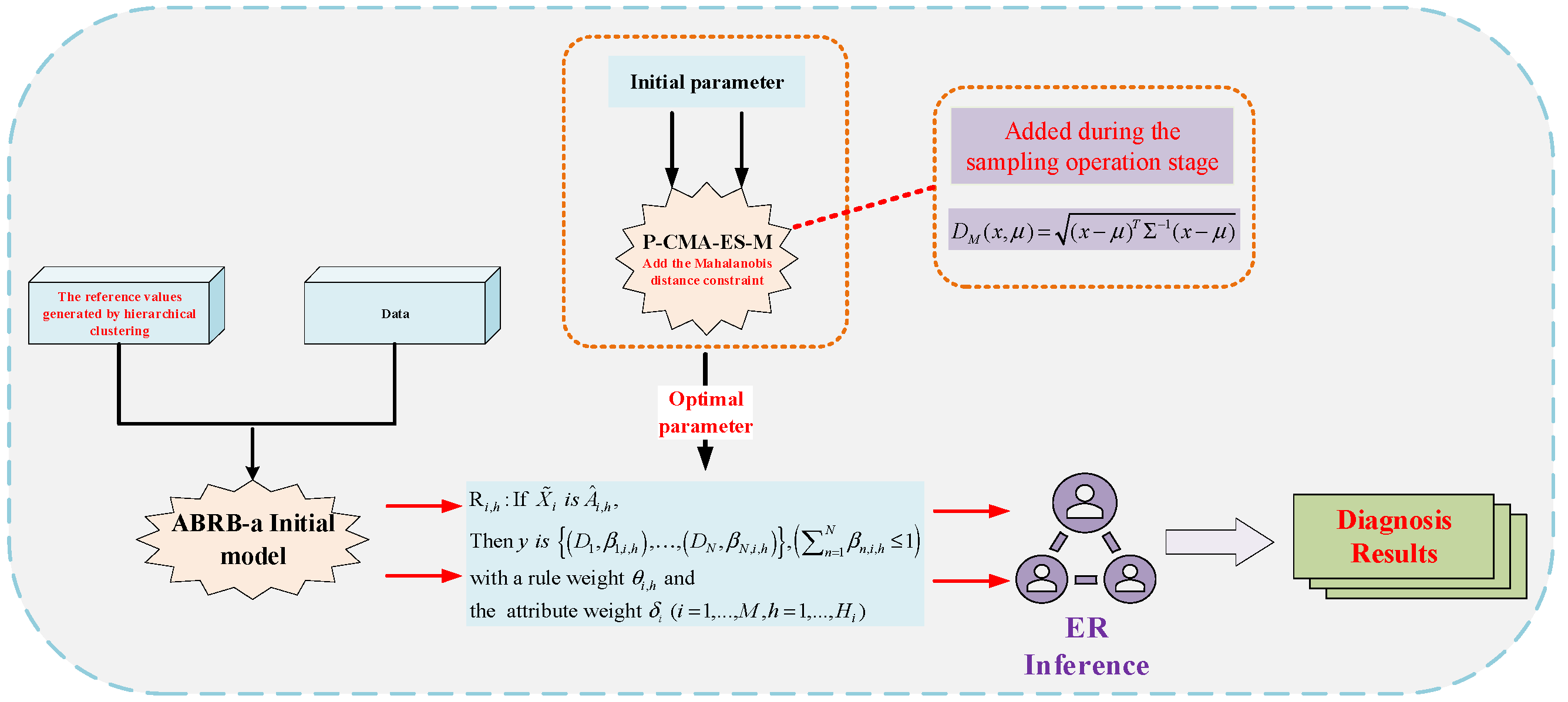
Figure 1. ABRB-a workflow diagram.
Symmetry 17 01687 g001
Figure 2. The specific process of agglomerative clustering.
Symmetry 17 01687 g002
Figure 3. Agglomerative clustering workflow.
Symmetry 17 01687 g003
Figure 4. P-CMA-ES-M optimization flowchart.
Symmetry 17 01687 g004
Figure 5. Feature importance.
Symmetry 17 01687 g005
Figure 6. Distribution of attributes values.
Symmetry 17 01687 g006
Figure 7. Distribution of result labels.
Symmetry 17 01687 g007
Figure 8. These are two confusion matrices. (a) Confusion matrix of ABRB model; (b) confusion matrix of ABRB-a model.
Symmetry 17 01687 g008
Figure 9. Comparison of the two prediction methods.
Symmetry 17 01687 g009
Figure 10. The accurate prediction of the EBRB model.
Symmetry 17 01687 g010
Figure 11. The accurate prediction of the IBRB model.
Symmetry 17 01687 g011
Figure 12. The accurate prediction of the SVM model.
Symmetry 17 01687 g012
Figure 13. The accurate prediction of the BP model.
Symmetry 17 01687 g013
Figure 14. The accurate prediction of the KNN model.
Symmetry 17 01687 g014
Figure 15. The accuracy performance of different models.
Symmetry 17 01687 g015
Figure 16. The precision performance of different models.
Symmetry 17 01687 g016
Figure 17. The Recall performance of different models.
Symmetry 17 01687 g017
Figure 18. The F1 performance of different models.
Symmetry 17 01687 g018
Figure 19. Comparison of MSE for different models.
Symmetry 17 01687 g019
Table 1. Meaning of attributes.
Symbol RepresentationMeaning
X1Past Exam Scores (PES)
X2Attendance Rate (AR)
X3Study Hours Per Week (SHPW)
X4Parental Education Level (PEL)
X5Extracurricular Activities (EA)
Table 2. Input reference values and attribute weight settings.
AttributeAttributeVLLMHVH
X111017.2524.531.7539
X2150.11762.579675.042387.50599.9677
X315062.57587.5100
X4100.751.52.253
X5100.250.50.751
Table 3. Output label settings.
Symbol RepresentationMeaning
0Pass(P)
1Fail(F)
Table 4. The initial model parameter settings based on ABRB-a.
NOAttributesRule
Weights
Reference
Values
Output Belief Degree
{P, F}
1PES
δ 1 = 1
1VL{0.6,0.4}
21L{0.1,0.9}
31M{0.8,0.2}
41H{0.3,0.7}
51VH{0.15,0.85}
6AR
δ 2 = 1
1VL{0.25,0.75}
71L{0.45,0.55}
81M{0.34,0.66}
91H{0.85,0.15}
101VH{0.95,0.05}
11SHPW
δ 3 = 1
1VL{0.33,0.67}
121L{1,0}
131M{0.55,0.45}
141H{0.15,0.85}
151VH{0,1}
16PEL
δ 4 = 1
1VL{0.2,0.8}
171L{0.7,0.3}
181M{0,1}
191H{1,0}
201VH{0.9,0.1}
21EA
δ 5 = 1
1VL{0.25,0.75}
221L{0.85,0.15}
231M{1,0}
241H{0.1,0.9}
251VH{0,1}
Table 5. The optimized model parameters result of ABRB-a.
NOAttributesRule
Weights
Reference
Values
Output Belief Degree
{P, F}
1PES
δ 1 = 0.8698
0.4041VL{0.03,0.97}
20.3041L{0.02,0.98}
30.2029M{0.1,0.9}
40H{0.84,0.16}
50.5407VH{0.01,0.99}
6AR
δ 2 = 0.2544
0.4793VL{0.03,0.97}
70.3358L{0,1}
80.0226M{0.34,0.66}
90.1463H{0.97,0.03}
10SHPW
δ 3 = 0.9559
0.8662VH{1,0}
110.9691VL{0.01,0.99}
120.3046L{0.02,0.98}
130M{0.08,0.92}
140.3008H{1,0}
150.9205VH{1,0}
16PEL
δ 4 = 0.4761
0.0293VL{0.2,0.8}
170.0158L{0.23,0.77}
180.1409M{0.01,0.99}
190.0728H{0.92,0.08}
200.0077VH{0.77,0.23}
21EA
δ 5 = 0.5652
0.1603VL{0,1}
220.0747L{0.4,0.6}
230.3699M{0.53,0.47}
240.4480H{0.58,0.42}
250.0313VH{0.87,0.13}
Table 6. Parameter settings of the comparison models.
ModelsParameter Settings
ABRB-a & BRBsBRBs use the same parameter settings as ABRB-a
KNNNumber of nearest neighbors = 200; Weight function = ‘uniform’; Weight function = ‘uniform’; Parameter in distance measurement = 2
SVMRegularization parameter = 5; Kernel function type= ‘rbf’; Coefficient of kernel function = ‘auto’; Constant term in kernel function = 0
BPNumber of neurons in hidden layers= [10, 2]; Activation function= ‘tansig’; Learning rate update strategy = ‘constant’; Maximum number of iterations = 10;
Note: BRBs refer to the ABRB, EBRB, and IBRB.
Table 7. Comparison of results from different models under the training set: test set ratio of 7:3.
Data PartitioningMethodmAccuracy (%)mPrecision (%)mRecall (%)mF1 (%)
Training:Testing
7:3
ABRB-a94.2794.4594.2894.25
ABRB79.5579.6479.6179.52
IBRB69.9572.4565.6468.64
EBRB75.4490.4057.5770.19
KNN81.0082.8677.0479.74
SVM87.4489.7997.787.28
BP73.3675.3874.3973.82
Table 8. Comparison of results from different models under the training set: test set ratio of 6:4.
Data PartitioningMethodmAccuracy (%)mPrecision (%)mRecall (%)mF1 (%)
Training:Testing
6:4
ABRB-a93.6493.7993.6393.63
ABRB78.9879.1279.0778.93
IBRB69.3763.3181.0671.1
EBRB73.2489.1652.4866.07
KNN78.1684.6270.2176.74
SVM86.6189.4586.0686.23
BP70.4277.6968.2472.66
Table 9. Comparison of results from different models under the training set: test set ratio of 8:2.
Data PartitioningMethodmAccuracy (%)mPrecision (%)mRecall (%)mF1 (%)
Training:Testing
8:2
ABRB-a94.7294.8294.6794.68
ABRB78.0878.0378.0477.90
IBRB71.1371.2168.1269.63
EBRB77.4697.8759.7474.19
KNN83.8076.1280.9578.46
SVM91.5493.0492.5792.24
BP80.2882.2670.8376.12
Table 10. Two types of distance constraints.
Distance ConstraintMSE
Mahalanobis0.1257
Euclidean0.1855
Table 11. Original data and performance under different disturbances.
Data TypesmAccuracy (%)mPrecision (%)mRecall (%)mF1 (%)
Raw data94.2794.4594.2894.25
P = 0.592.392.5292.2892.25
P = 0.788.6888.0888.0287.73
Table 12. Verification of the generalization ability of the ABRB-a model.
MethodmAccuracy (%)mPrecision (%)mRecall (%)mF1 (%)
ABRB-a9596.1694.6694.65
ABRB83.7885.9184.5183.23
IBRB74.7674.0960.8561.21
EBRB70.9478.4480.0779.01
KNN69.7255.553.3253.78
SVM64.0451.9041.9643.92
BP73.0556.1953.6452.41
Disclaimer/Publisher’s Note: The statements, opinions and data contained in all publications are solely those of the individual author(s) and contributor(s) and not of MDPI and/or the editor(s). MDPI and/or the editor(s) disclaim responsibility for any injury to people or property resulting from any ideas, methods, instructions or products referred to in the content.