Fractional-Order Numerical Scheme with Symmetric Structure for Fractional Differential Equations with Step-Size Control

Abstract

This research paper uses two-stage explicit fractional numerical schemes to solve fractional-order initial value problems of ODEs. The proposed methods exhibit structural symmetry in their formulation, contributing to enhanced numerical stability and balanced error behavior across computational steps. The schemes utilize constant and variable step sizes, allowing them to adapt efficiently to solve the considered fractional-order initial value problems. These schemes employ variable step-size control based on error estimation, aiming to minimize computational costs while maintaining good accuracy and stability. We discuss the linear stability of the proposed numerical schemes and observe that a higher-stability region is obtained when the fractional parameter value equals one. We also discuss consistency and convergence analysis of the proposed methods and observe that as the fractional parameter values rise from 0 to 1, the scheme’s convergence rate improves and achieves its maximum at 1. Several numerical test problems are used to demonstrate the efficiency of the proposed methods in solving fractional-order initial value problems with either constant or variable step sizes. The proposed numerical schemes’ results demonstrate better accuracy and convergence behavior than the existing methods used for comparison.

1. Introduction

Fractional calculus [1,2], which employs derivatives and integrals of arbitrary (non-integer) order, has received a lot of attention for its ability to mimic complex systems with memory, non-locality, and intrinsic symmetry features that are normally beyond the scope of classical calculus. Fractional calculus has been applied in various scientific and engineering fields, including control theory [3], signal processing [4], fluid dynamics [5], viscoelasticity [6], and bioengineering [7]. Fractional differential equations, for instance, describe anomalous diffusion in porous media, which is crucial to groundwater flow and oil recovery [8].

Additionally, in electrical engineering, fractional models describe the behavior of capacitors and inductors in non-ideal circuits. They are also significant for biomedical applications, as they aid in simulating the intricate dynamics of biological model problems and neural activity. Improvements in numerical methods are making fractional calculus more useful in solving nonlinear differential equations, paving the way for new developments in scientific and engineering computation. Symmetric formulations in numerical analysis usually result in improved stability, error distribution, and computing efficiency. Preserving or exploiting such symmetry in numerical algorithms often leads to greater stability, balanced error propagation, and improved computational efficiency. Due to its flexibility, fractional calculus is essential for scholars and practitioners grappling with the complexities of modern times.

Due to fractional calculus’s ability to model a wide range of complex phenomena from various domains, such as fluid flow, electrical circuits, biological systems, and viscoelasticity, which frequently exhibit temporal or spatial symmetry, where conventional integer-order models fall short, the study of fractional initial value problems has garnered significant attention. Fractional initial value problems (FIVPs) are closely related to fractional-order differential equations (FODEs), which are differential equations defined using fractional derivatives [9]:

$$\left.\begin{array}{c}{⅁}^{[¢]}y\left(t\right)=f\left(t,y\left(t\right)\right),\\ y^{\left(k\right)}\left(t_0\right)=y_0^{\left(k\right)},k=0,1,\dots ,m-1,\end{array}\right\}$$

(1)

where

$${⅁}^{[¢]}y\left(t\right)={\displaystyle \frac{1}{\Gamma \left(m-¢\right)}}\underset{t_0}{\stackrel{t}{\int }}{\displaystyle \frac{y^{\left(m\right)}\left(h\right)dh}{{\left(t-h\right)}^{¢-m+1}}},m-1<¢<m\in {\mathbb{Z}}^{+},$$

(2)

is the Caputo fractional derivative of order ¢ and $t\in \left[t_0,t_n\right].$ These FIVPs provide a more adaptable and realistic representation of dynamic systems, especially those that involve memory effects or long-range interactions. While reasonable analytical solutions to these problems can be obtained in only a few cases by using basic equations, such as series expansions, they may quickly become computationally expensive for more complex systems. Consequently, numerical methods have emerged as highly efficient and accurate solutions to FIVPs. The two-stage fractional-order explicit approaches are advantageous due to their simplicity, versatility, and ability to handle nonlinearities. Numerical schemes, particularly when combined with adaptive step-size strategies, address the challenges posed by analytical methods and provide both robustness and computational efficiency across a wide range of applications, as mentioned below:

• They have a lower computational cost because of their phased strategy, which optimizes calculations at each step while retaining accuracy.
• They minimize CPU time by reducing redundant computations, especially with adaptive step-size control and efficient implementations.
• Using fractional derivatives in iterative processes leads to faster convergence than existing methods.
• The efficient two-stage structure requires fewer functional evaluations per iteration, lowering overall computational cost.
• They have modest algorithmic complexity, ranging from simple, nonadaptive procedures to more complicated, adaptive strategies.
• Robust for numerous FIVPs and complex problems with strong nonlinear or singular behavior.
• They provide better-than-average control over local and global errors through repeated refining and dynamically changing step sizes.
• Memory efficient, as big arrays or matrices are avoided, particularly in adaptive implementation.
• They are adaptable and include various stopping criteria, such as error tolerance and step-size control, which offer improved accuracy for the considered FIVPs.

The fractional two-stage approach is distinguished by its balance of accuracy and efficiency, making it a suitable numerical method for solving FIVPs. To solve FIVPs in [10], the fractional Euler method is proposed as follows:

$$y_{j+1}=y_j+{\displaystyle \frac{h^{¢}}{\Gamma \left(¢+1\right)}}f\left(t_j,y_j\right),$$

(3)

where $h=t_{j+1}-t_j$ is the step size. The aforementioned Euler scheme’s local truncation error is $O\left({\displaystyle \frac{h^{2¢}}{\Gamma \left(2¢+1\right)}}\right)$, suggesting lower-order precision in approximating fractional-order derivatives. These restrictions have an impact on solution precision, especially for stiff or highly nonlinear problems. To address this, Batiha et al. [11] proposed a better approach with enhanced convergence capabilities, i.e.,

$$y_{j+1}=y_j+{\displaystyle \frac{h¢}{\Gamma \left(¢+1\right)}}{k}_{4,}$$

(4)

$$\left.\begin{array}{c}{k}_1=f\left(t_j,y_j\right),\\ k_2=f\left(t_j,y_j+\left({\displaystyle \frac{h^{¢}}{\Gamma \left(¢+1\right)}}\right)k_1\right),\\ k_3=f\left(t_j,y_j+\left({\displaystyle \frac{h^{¢}}{\Gamma \left(¢+1\right)}}\right)k_2\right),\\ k_4=f\left(t_j,y_j+\left({\displaystyle \frac{h^{¢}}{\Gamma \left(¢+1\right)}}\right)k_3\right),\end{array}\right\}$$

(5)

with the following local truncation error:

$$\begin{array}{cc}\hfill y\left(t_j\right)-y_{j+1}& \approx \left({\displaystyle \frac{1}{12}}f{D}_{ty}^{[¢]}f+{\displaystyle \frac{1}{2}}{f}^2{D}_{yy}^{[¢]}f+{\displaystyle \frac{1}{6}}{D}_t^{[¢]}f{D}_y^{[¢]}f-{\displaystyle \frac{1}{24}}{D}_{tt}^{[¢]}f\right.\hfill \\ \hfill & \left.-{\displaystyle \frac{1}{3}}f{\left(D_y^{[¢]}f\right)}^2\right)\left({\displaystyle \frac{h^{3¢}}{\Gamma \left(3¢+1\right)}}\right)+O\left({\displaystyle \frac{h^{4¢}}{\Gamma \left(4¢+1\right)}}\right)D^{[3¢]}\left(y\left(\zeta \right)\right),\hfill \end{array}$$

(6)

where the operator $D_{t,y}^{[¢]}f$ denotes the Caputo fractional derivative of order ¢ of the function f with respect to the variables $t,y$. Thus, for ${\displaystyle \frac{h^{3¢}}{\Gamma \left(3¢+1\right)}}$, the error is

$$O\left({\displaystyle \frac{h^{4¢}}{\Gamma \left(4¢+1\right)}}\right)D^{[3¢]}\left(y\left(\zeta \right)\right).$$

The fractional version in [12] is given as

$$y_{j+1}=y_j+{\displaystyle \frac{h^{¢}}{\Gamma \left(¢+1\right)}}{\displaystyle \frac{{\left(k_1\right)}^2+{\left(k_2\right)}^2}{k_1+k_2}},$$

(7)

$$\left.\begin{array}{c}{k}_1=f\left(t_j,y_j\right),\\ k_2=f\left(t_j,y_j+{\displaystyle \frac{h^{¢}}{\Gamma \left(¢+1\right)}}{k}_1\right).\end{array}\right\}$$

(8)

The local truncation error of the aforementioned fractional scheme is computed as a function of the deviation induced at each step. It illustrates how well the scheme approximates the true solution to the fractional differential equation. It is critical to examine the error in order to evaluate the proposed methods’ reliability and consistency.

$$\begin{array}{cc}\hfill y\left(t_j\right)-y_{j+1}& \approx \left({\displaystyle \frac{1}{6}}f{D}_{ty}^{[¢]}f-{\displaystyle \frac{1}{12}}{f}^2{D}_{yy}^{[¢]}f-{\displaystyle \frac{1}{3}}{D}_t^{[¢]}f{D}_y^{[¢]}f-{\displaystyle \frac{1}{4}}{\displaystyle \frac{{\left(D_{ty}^{[¢]}f\right)}^2}{f}}-{\displaystyle \frac{1}{12}}f{\left(D_y^{[¢]}f\right)}^2\right)\hfill \\ \hfill & \times \left({\displaystyle \frac{h^{3¢}}{\Gamma \left(3¢+1\right)}}\right)+O\left({\displaystyle \frac{h^{4¢}}{\Gamma \left(4¢+1\right)}}\right)D^{[3¢]}\left(y\left(\zeta \right)\right).\hfill \end{array}$$

(9)

Some researchers have developed various numerical methods for solving ordinary and fractional differential equations, as reported in [13,14,15,16,17] and the references cited therein. To solve FIVPs, most fractional methods rely on a fixed step size throughout the integration process. In particular, to maintain precision, very small step sizes are typically required, which significantly increases the cost and memory usage.

Motivated by the established advantages of fractional-order schemes and the need for enhanced accuracy, this paper aims to develop a robust family of two-stage fractional-order numerical methods for solving (1). A variable-step-size technique is introduced to address the drawbacks of constant-step-size approaches. It performs dynamic adjustments during integration based on local error estimates. Besides improving computational efficiency by allowing for larger steps during smoother intervals, this adaptive method ensures greater accuracy in regions with rapid changes in the solution. Additionally, the adaptive nature of this approach prevents instability and significantly enhances accuracy, especially when solving complex problems.

This paper is structured as follows: Section 2 develops two-stage fractional-order schemes and provides a theoretical analysis of the proposed methods. The implementation and performance of the proposed methods, along with a comparison with some existing methods, are reported in Section 3 using a few fractional-order IVPs. The paper is concluded in Section 4.

2. Development of Novel Fractional Schemes

We begin by introducing essential definitions and concepts necessary for understanding the considered FIVPs, focusing on the Caputo fractional derivative, which is preferred for dealing with fractional-order differential equations because it satisfies initial conditions, such as $\left[{⅁}^{[¢]}\right]\left(c\right)=0$, and defines the Riemann–Liouville integral operator of order ¢ as reported in [18]:

$$J^{[¢]}\left[f\left(x\right)\right]={\displaystyle \frac{1}{\Gamma ¢}}\stackrel{x}{\underset{0}{\int }}\left({\left(x-t\right)}^{¢-1}f\left(t\right)\right)dt,x>0,¢\in \left(0,1\right]$$

(10)

The following characteristics hold:

• –

  $J^{\left[{¢}_1^{[\ast ]}\right]}{J}^{\left[{¢}_2^{[\ast ]}\right]}\left[f\left(x\right)\right]=J^{\left[{¢}_2^{[\ast ]}\right]}{J}^{\left[{¢}_1^{[\ast ]}\right]}\left[f\left(x\right)\right],{¢}_1^{[\ast ]},{¢}_2^{[\ast ]}>0;$

  –

  $J^{\left[{¢}_1^{[\ast ]}\right]}{J}^{\left[{¢}_2^{[\ast ]}\right]}\left[f\left(x\right)\right]=J^{\left[{¢}_1^{[\ast ]}\right]+\left[{¢}_2^{[\ast ]}\right]}\left[f\left(x\right)\right],{¢}_1^{[\ast ]},{¢}_2^{[\ast ]}>0;$

  –

  $J^{\left[{¢}_1^{[\ast ]}\right]}{x}^{\kappa }={\displaystyle \frac{\Gamma \left(¢+\kappa \right)}{\Gamma \left(¢+\kappa +1\right)}}{x}^{\kappa +\left[{¢}_1^{[\ast ]}\right]},\kappa >-1.$

Lemma 1

([19]). If $f\in C^n[0,b],x>0,$ and $n-1<¢\le n,$ such that $n\in \mathbb{N},$ we have

$${⅁}^{[¢]}{J}^{[¢]}\left[f\left(x\right)\right]=f\left(x\right),$$

(11)

and

$$J{\ast }^{[¢]}\left({⅁}^{[¢]}\left[f\left(x\right)\right]\right)=f\left(x\right)-\sum _{s=0}^{n-1}{f}^s\left(0^{+}\right){\displaystyle \frac{x^s}{s!}}.$$

(12)

Lemma 1 follows from the standard properties of Caputo fractional derivatives and fractional integrals: Equation (11) shows that the derivative of the fractional integral returns the original function, while Equation (12) recovers the function up to a polynomial determined by initial values. These results are well-established in [20].

Theorem 1

(Generalized Taylor Formula for Caputo Derivatives). In the context of Caputo fractional derivatives, a function $f\left(t\right)$ can be expanded around a node $t_0$ using a fractional Taylor series. This expansion provides an approximate representation of $f\left(t\right)$ and plays a key role in analyzing the convergence of fractional numerical schemes.

Specifically, for $¢\in (0,1]$ and $f\in C^n[0,t_n]$, the fractional Taylor formula is given by [21]

$$f\left(t\right)=\sum _{i=0}^n{\displaystyle \frac{{\left(t-t_0\right)}^{i¢}}{\Gamma \left(i¢+1\right)}}{⅁}^{[i¢]}f\left(t_o\right)+{\displaystyle \frac{{\left(t-t_0\right)}^{\left(n+1\right)¢}}{\Gamma \left(\left(n+1\right)¢+1\right)}}{⅁}^{[\left(n+1\right)¢]}f\left(\zeta \right),0<\zeta <t,$$

(13)

where ${⅁}^{[s¢]}f\left(t\right)$ denotes the Caputo derivative of order s¢, for $s=0,1,2,\dots ,n.$ In expanded form, the series can be written as

$$f\left(t\right)=\left[\begin{array}{c}f\left(t_0\right)+{\displaystyle \frac{{\left(t-t_0\right)}^{¢}}{\Gamma \left(¢+1\right)}}{⅁}^{[¢]}f\left(t_0\right)+{\displaystyle \frac{{\left(t-t_0\right)}^{2¢}}{\Gamma \left(2¢+1\right)}}{⅁}^{[2¢]}f\left(t_0\right)+\dots +\\ {\displaystyle \frac{{\left(t-t_0\right)}^{i¢}}{\Gamma \left(i¢+1\right)}}{⅁}^{[i¢]}f\left(t_0\right)+{\displaystyle \frac{{\left(t-t_0\right)}^{\left(n+1\right)¢}}{\Gamma \left(\left(n+1\right)¢+1\right)}}{⅁}^{[\left(n+1\right)¢]}f\left(\zeta \right).\end{array}\right]$$

(14)

Equation (14) is used to calculate the error of fractional-order algorithms to solve FIVPs.

For fractional-order IVPs, the general form of a fractional-order second-stage Runge–Kutta method is often employed because of its simplicity and higher accuracy compared with lower-order fractional schemes. To improve the stability and accuracy of the solution, we evaluate the function at intermediate points within each phase. The mathematical formulation of this method is provided as [22]

$$y_{j+1}=y_j+{\displaystyle \frac{h^{¢}}{\Gamma \left(¢+1\right)}}\wp \left(t_j,y_j;{\displaystyle \frac{h^{¢}}{\Gamma \left(¢+1\right)}}\right),$$

(15)

where

$$\wp \left(t_j,y_j;{\displaystyle \frac{h^{¢}}{\Gamma \left(¢+1\right)}}\right)=\sum _{i=1}^m{\omega }_i{k}_i$$

(16)

with

$$\left.\begin{array}{c}{k}_1=f\left(t_j,y_j\right),\\ k_i=f\left(t_j+c_i{\displaystyle \frac{h^{¢}}{\Gamma \left(¢+1\right)}},y_j+{\displaystyle \frac{h^{¢}}{\Gamma \left(¢+1\right)}}\sum _{j=1}^{i-1}{\alpha }_{ij}{k}_j\right),\end{array}\right\}$$

(17)

where $c_i={\sum }_{j=1}^{i-1}{\alpha }_{ij},i=2.$ For some particular values of ${\sum }_{i=1}^m{\omega }_i,$$c_i$ and ${\sum }_{j=1}^{i-1}{\alpha }_{ij},$ we have the well-known midpoint method [23]:

$$y_{j+1}=y_j+{\displaystyle \frac{h^{¢}}{2\Gamma \left(¢+1\right)}}\left(k_1+k_2\right),$$

(18)

where

$$\left.\begin{array}{c}{k}_1=f\left(t_j,y_j\right),\\ k_2=f\left(t_j+{\displaystyle \frac{h^{¢}}{\Gamma \left(¢+1\right)}},y_j+{\displaystyle \frac{h^{¢}}{\Gamma \left(¢+1\right)}}{k}_1\right).\end{array}\right\}$$

(19)

We abbreviated the method as ${\mathrm{RMFS}}_1^{[\ast ]}$, and it satisfies the local truncation error (L.T.E)

$$\begin{array}{cc}\hfill L.T.E& =\left(-{\displaystyle \frac{1}{12}}{⅁}_{xx}^{[¢]}f-{\displaystyle \frac{1}{6}}f{⅁}_{ty}^{[¢]}f-{\displaystyle \frac{1}{12}}{f}^2{⅁}_{yy}^{[¢]}f+{\displaystyle \frac{1}{6}}f{\left({⅁}_y^{[¢]}f\right)}^2+{\displaystyle \frac{1}{6}}{⅁}_t^{[¢]}f{⅁}_y^{[¢]}f\right)\hfill \\ \hfill & \times {\displaystyle \frac{h^{3¢}}{\Gamma \left(3¢+1\right)}}+O\left({\displaystyle \frac{h^{4¢}}{\Gamma \left(4¢+1\right)}}\right){⅁}^{[3¢]}\left(y\left(\zeta \right)\right),\hfill \end{array}$$

(20)

and the order of convergence is ${\displaystyle \frac{h^{2¢}}{\Gamma \left(2¢+1\right)}}.$ The developed method is consistent, since

$$\underset{h\to 0}{lim}\Phi \left(t_j,y_j,{\displaystyle \frac{h^{¢}}{\Gamma \left(¢+1\right)}}\right)=f\left(t_j,y_j\right),$$

therefore,

$$\begin{array}{ccc}\hfill \underset{h\to 0}{lim}\Phi \left(t_j,y_j,{\displaystyle \frac{h^{¢}}{\Gamma \left(¢+1\right)}}\right)& =& \underset{h\to 0}{lim}\left({\displaystyle \frac{f\left(t_j,y_j\right)+f\left(t_j+\frac{h^{¢}}{\Gamma \left(¢+1\right)},y_j+\frac{h^{¢}}{\Gamma \left(¢+1\right)}{k}_2\right)}{2}}\right),\hfill \\ & =& f\left(t_j,y_j\right).\hfill \end{array}$$

(21)

The Modified Fractional Euler method [24] is defined as follows:

$$y_{j+1}=y_j+{\displaystyle \frac{h^{¢}}{\Gamma \left(¢+1\right)}}{k}_2,$$

(22)

where

$$\left.\begin{array}{c}{k}_1=f\left(t_j,y_j\right),\\ k_2=f\left(t_j+{\displaystyle \frac{1}{2}}{\displaystyle \frac{h^{¢}}{\Gamma \left(¢+1\right)}},y_j+{\displaystyle \frac{1}{2}}{\displaystyle \frac{h^{¢}}{\Gamma \left(¢+1\right)}}{k}_1\right).\end{array}\right\}$$

(23)

We abbreviated the method as ${\mathrm{RMFS}}_2^{[\ast ]}$, and it satisfies the local truncation error

$$\begin{array}{cc}\hfill L.T.E& =\left({\displaystyle \frac{1}{24}}{⅁}_{tt}^{[¢]}f+{\displaystyle \frac{1}{12}}f{⅁}_{ty}^{[¢]}f+{\displaystyle \frac{1}{24}}{f}^2{⅁}_{yy}^{[¢]}f+{\displaystyle \frac{1}{6}}f{\left({⅁}_y^{[¢]}f\right)}^2+{\displaystyle \frac{1}{6}}{⅁}_t^{[¢]}f{⅁}_y^{[¢]}f\right)\hfill \\ \hfill & \times {\displaystyle \frac{h^{3¢}}{\Gamma \left(3¢+1\right)}}+O\left({\displaystyle \frac{h^{4¢}}{\Gamma \left(4¢+1\right)}}\right){⅁}^{[3¢]}\left(y\left(\zeta \right)\right),\hfill \end{array}$$

(24)

and the obtained order of convergence is ${\displaystyle \frac{h^{2¢}}{\Gamma \left(2¢+1\right)}}.$ The developed method is consistent, since

$$\underset{h\to 0}{lim}\wp \left(t_j,y_j,{\displaystyle \frac{h^{¢}}{\Gamma \left(¢+1\right)}}\right)=f\left(t_j,y_j\right),$$

(25)

therefore

$$\begin{array}{ccc}\hfill \underset{h\to 0}{lim}\wp \left(t_j,y_j,{\displaystyle \frac{h^{¢}}{\Gamma \left(¢+1\right)}}\right)& =& \underset{h\to 0}{lim}\left(f\left(t_j+{\displaystyle \frac{h^{¢}}{2\Gamma \left(¢+1\right)}},y_j+{\displaystyle \frac{h^{¢}}{2\Gamma \left(¢+1\right)}}{k}_1\right)\right),\hfill \\ & =& f\left(t_j,y_j\right).\hfill \end{array}$$

(26)

Fractional-order methods are essential because they account for the memory and hereditary effects present in many physical, biological, and engineering systems. Their ability to depict non-local dynamics makes them excellent for simulating real-world processes with complex temporal behavior. Unlike classical methods, these approaches effectively model complex phenomena such as anomalous diffusion and viscoelasticity, especially with power-law behavior. Their ability to precisely capture the non-local and history-dependent dynamics of fractional systems enables a deeper understanding of natural phenomena.

2.1. Construction and Convergence Analysis of the Fractional Schemes

Here, we illustrate the construction of the proposed fractional schemes and analyze their convergence for Caputo-type fractional initial value problems. Consider

$$y\left(x\right)=y\left(x_j\right)+\stackrel{x}{\underset{x_j}{\int }}{y}^{\prime }\left(t\right)⅁t.$$

(27)

Using a hybrid quadrature rule, we approximate (27) as

$$\stackrel{x}{\underset{x_j}{\int }}{y}^{\prime }\left(t\right)⅁t\approx {\displaystyle \frac{x-x_j}{m}}\sum _{i=1}^m{y}^{\prime }\left(x_j+\left(x-x_j\right)\left({\displaystyle \frac{2i-1}{2m}}\right)\right).$$

(28)

Formula (28) is derived by applying a hybrid quadrature rule to approximate the integral in (27). In particular, the interval $\left[x_j,x\right]$ is subdivided into m equal sub-intervals, and the midpoint rule is employed within each sub-interval. This choice balances accuracy with computational efficiency, as the midpoint rule is known to be second-order-accurate. From the perspective of error analysis, the approximation can be expressed as

$$\stackrel{x}{\underset{x_j}{\int }}{y}^{\prime }\left(t\right)⅁t\approx {\displaystyle \frac{x-x_j}{m}}\sum _{i=1}^m{y}^{\prime }\left(x_j+\left(x-x_j\right)\left({\displaystyle \frac{2i-1}{2m}}\right)\right)+O\left({\displaystyle \frac{{\left(x-x_j\right)}^3}{m^2}}\right).$$

(29)

Hence, the truncation error introduced by (28) is of order $O\left(h^2\right)$, which vanishes as $h\to \infty .$ Therefore, the approximation is consistent with the Taylor series expansion and ensures the accuracy required for constructing the proposed fractional schemes. From (1)–(6) and (27)–(28), we define the following fractional scheme as

$$y_{j+1}=y_j+\left({\displaystyle \frac{h^{¢}}{\Gamma \left(¢+1\right)}}\right)\wp \left(t_j,y_j;{\displaystyle \frac{h^{¢}}{\Gamma \left(¢+1\right)}}\right),$$

(30)

where

$$\wp \left(t_j,y_j;{\displaystyle \frac{h^{¢}}{\Gamma \left(¢+1\right)}}\right)=\sum _{i=1}^m{\omega }_i{k}_i+{\displaystyle \frac{k_1{k}_2}{k_1+k_2}},$$

(31)

and

$$\left.\begin{array}{c}{k}_1=f\left(t_j,y_j\right),\\ k_i=f\left(t_j+c_i{\displaystyle \frac{h^{¢}}{\Gamma \left(¢+1\right)}},y_j+{\displaystyle \frac{h^{¢}}{\Gamma \left(¢+1\right)}}\sum _{j=1}^{i-1}{\alpha }_{ij}{k}_j\right).\end{array}\right\}$$

(32)

Using (32), we determine the unknown parameters ${\omega }_1,{\omega }_2,$$c_2$, and ${\alpha }_{21}$ to agree with the Taylor series method of the highest possible term. Then, we use the generalized Taylor series expansion as follows:

$$\begin{array}{cc}\hfill y\left(t_{j+1}\right)& =y_j+{\displaystyle \frac{h^{¢}}{\Gamma \left(¢+1\right)}}f+\left({\displaystyle \frac{1}{2}}{⅁}_t^{[¢]}f+{\displaystyle \frac{1}{2}}f{⅁}_y^{[¢]}f\right){\displaystyle \frac{h^{2¢}}{\Gamma \left(2¢+1\right)}}+\left({\displaystyle \frac{1}{6}}{⅁}_{tt}^{[¢]}f\right.\hfill \\ \hfill & \left.+{\displaystyle \frac{1}{3}}f{⅁}_{ty}^{[¢]}f+{{\displaystyle \frac{1}{6}}}^2{⅁}_{yy}^{[¢]}f+{\displaystyle \frac{1}{6}}{⅁}_t^{[¢]}f{⅁}_y^{[¢]}+{\displaystyle \frac{1}{6}}f{\left({⅁}_y^{[¢]}f\right)}^2\right){\displaystyle \frac{h^{3¢}}{\Gamma \left(3¢+1\right)}}+\dots \hfill \end{array}$$

(33)

By computing the Taylor series expansion of $k_1$ and $k_i,$ we have

$$k_1=f,$$

(34)

$$\begin{array}{cc}\hfill k_2& =f+\left(c_2{⅁}_t^{[¢]}f+{\alpha }_{21}f{⅁}_y^{[¢]}f\right){\displaystyle \frac{h^{¢}}{\Gamma \left(¢+1\right)}}+\left({\displaystyle \frac{1}{2}}{f}^2{⅁}_{yy}^{[¢]}f{\alpha }_{21}^2+f{⅁}_{ty}^{[¢]}f{c}_2{\alpha }_{21}\right.\hfill \\ \hfill & \left.+{\displaystyle \frac{1}{2}}{c}_2^2{⅁}_{tt}^{[¢]}f\right){\displaystyle \frac{h^{2¢}}{\Gamma \left(2¢+1\right)}}+\left({\displaystyle \frac{1}{6}}{f}^3{⅁}_{yyy}^{[¢]}f{\alpha }_{21}^3+{\displaystyle \frac{1}{2}}{f}^2{⅁}_{tyy}^{[¢]}f{c}_2{\alpha }_{21}^2+{\displaystyle \frac{1}{2}}f{⅁}_{tty}^{[¢]}f{c}_2^2{\alpha }_{21}\right.\hfill \\ \hfill & \left.+{\displaystyle \frac{1}{6}}{⅁}_{ttt}^{[¢]}f{c}_2^3\right){\displaystyle \frac{h^{3¢}}{\Gamma \left(3¢+1\right)}}+O\left({\displaystyle \frac{h^{4¢}}{\Gamma \left(4¢+1\right)}}\right){⅁}^{[3¢]}\left(y\left(\zeta \right)\right).\hfill \end{array}$$

(35)

Thus,

$$\begin{array}{cc}\hfill {\omega }_1{k}_1& +{\displaystyle \frac{k_1{k}_2}{k_1+k_2}}+{\omega }_2{k}_2={\omega }_{1}f+{\displaystyle \frac{1}{2}}f+{\omega }_{2}f+\left({\displaystyle \frac{1}{4}}{⅁}_t^{[¢]}f{c}_2+{\displaystyle \frac{1}{4}}f{⅁}_y^{[¢]}f{\alpha }_{21}\right.\hfill \\ \hfill & \left.+{\omega }_2\left(c_2{⅁}_t^{[¢]}f+{\alpha }_{21}f{⅁}_y^{[¢]}\right)\right)\left({\displaystyle \frac{h^{¢}}{\Gamma \left(¢+1\right)}}\right)+\left({\displaystyle \frac{1}{2f}}\left({\displaystyle \frac{1}{2}}f\left({\displaystyle \frac{1}{2}}{f}^2{⅁}_{yy}^{[¢]}f{\alpha }_{21}^2\right.\right.\right.\hfill \\ \hfill & \left.+c_2{\alpha }_{21}^{2}f{⅁}_{ty}^{[¢]}f+{\displaystyle \frac{1}{2}}{c}_2^2{⅁}_{tt}^{[¢]}f\right)+\left(-{\displaystyle \frac{1}{4}}{c}_2{⅁}_t^{[¢]}f-{\displaystyle \frac{1}{4}}{\alpha }_{21}f{⅁}_y^{[¢]}f\right)\left(c_2{⅁}_t^{[¢]}f\right.\hfill \\ \hfill & \left.\left.\left.+{\alpha }_{21}f{⅁}_y^{[¢]}f\right)\right)+{\omega }_2\left(\begin{array}{c}{\displaystyle \frac{1}{2}}{f}^2{⅁}_{yy}^{[¢]}f{\alpha }_{21}^2+\\ f{⅁}_{ty}^{[¢]}f{\alpha }_{21}{c}_2\\ +{\displaystyle \frac{1}{2}}{c}_2^2{⅁}_{tt}^{[¢]}f\end{array}\right)\right)\left({\displaystyle \frac{h^{2¢}}{\Gamma \left(2¢+1\right)}}\right)+\dots \hfill \end{array}$$

(36)

By substituting (36) into (30) and comparing the coefficients of ${\displaystyle \frac{h^{¢}}{\Gamma \left(¢+1\right)}}f$, ${\displaystyle \frac{h^{2¢}}{\Gamma \left(2¢+1\right)}}{⅁}_t^{[¢]}f$, and ${\displaystyle \frac{h^{2¢}}{\Gamma \left(2¢+1\right)}}f{⅁}_y^{[¢]}f$ with the corresponding terms in the Taylor series expansion (33), we obtain the following relations:

$${\omega }_1+{\omega }_2={\displaystyle \frac{1}{2}},$$

(37)

$$\left({\displaystyle \frac{1}{4}}+{\omega }_2\right)c_2={\displaystyle \frac{1}{2}},$$

(38)

$$\left({\displaystyle \frac{1}{4}}+{\omega }_2\right){\alpha }_{21}={\displaystyle \frac{1}{2}}.$$

(39)

By solving the system in (37)–(39), we have the following schemes for ${\omega }_1=-{\displaystyle \frac{1}{2}},{\omega }_2=1$, and $c_2={\alpha }_{21}={\displaystyle \frac{2}{5}}$:

$$y_{j+1}=y_j+{\displaystyle \frac{h^{¢}}{\Gamma \left(¢+1\right)}}\left({\displaystyle \frac{2k_2-k_1}{2}}+{\displaystyle \frac{k_1{k}_2}{k_1+k_2}}\right),$$

(40)

where

$$\left.\begin{array}{c}{k}_1=f\left(t_j,y_j\right),\\ k_2=f\left(t_j+{\displaystyle \frac{2}{5}}{\displaystyle \frac{h^{¢}}{\Gamma \left(¢+1\right)}},y_j+{\displaystyle \frac{h^{¢}}{\Gamma \left(¢+1\right)}}{\displaystyle \frac{2}{5}}{k}_2\right).\end{array}\right\}$$

We abbreviated the method as ${\mathrm{RMFS}}_3^{[\ast ]}$, and it satisfies the local truncation error (L.T.E)

$$\begin{array}{cc}\hfill L.T.E& =\left({\displaystyle \frac{1}{15}}{⅁}_{tt}^{[¢]}f+{\displaystyle \frac{2}{15}}f{⅁}_{ty}^{[¢]}f+{\displaystyle \frac{1}{15}}{f}^2{⅁}_{yy}^{[¢]}f+{\displaystyle \frac{14}{75}}f{\left({⅁}_y^{[¢]}f\right)}^2+{\displaystyle \frac{31}{150}}{⅁}_t^{[¢]}f{⅁}_y^{[¢]}f\right.\hfill \\ \hfill & \left.+{\displaystyle \frac{1}{50f}}{\left({⅁}_t^{[¢]}f\right)}^2\right){\displaystyle \frac{h^{3¢}}{\Gamma \left(3¢+1\right)}}+O\left({\displaystyle \frac{h^{4¢}}{\Gamma \left(4¢+1\right)}}\right){⅁}^{[3¢]}\left(y\left(\zeta \right)\right),\hfill \end{array}$$

(41)

and the obtained order of convergence is ${\displaystyle \frac{h^{2¢}}{\Gamma \left(2¢+1\right)}}.$ The developed method in (40) is consistent, since

$$\underset{h\to 0}{lim}\wp \left(t_j,y_j,{\displaystyle \frac{h^{¢}}{\Gamma \left(¢+1\right)}}\right)=f\left(t_j,y_j\right),$$

therefore,

$$\begin{array}{cc}\hfill \underset{h\to 0}{lim}\wp \left(t_j,y_j,{\displaystyle \frac{h^{¢}}{\Gamma \left(¢+1\right)}}\right)& =\underset{h\to 0}{lim}\left({\displaystyle \frac{2\left(f\left(t_j+\frac{2}{5}\frac{h^{¢}}{\Gamma \left(¢+1\right)},y_j+\frac{h^{¢}}{\Gamma \left(¢+1\right)}\frac{2}{5}{k}_2\right)\right)-f\left(t_j,y_j\right)}{2}}\right.\hfill \\ \hfill & \left.+{\displaystyle \frac{f\left(t_j,y_j\right)\left(f\left(t_j+\frac{2}{5}\frac{h^{¢}}{\Gamma \left(¢+1\right)},y_j+\frac{h^{¢}}{\Gamma \left(¢+1\right)}\frac{2}{5}{k}_2\right)\right)}{\left(f\left(t_j,y_j\right)\right)+\left(f\left(t_j+\frac{2}{5}\frac{h^{¢}}{\Gamma \left(¢+1\right)},y_j+\frac{h^{¢}}{\Gamma \left(¢+1\right)}\frac{2}{5}{k}_2\right)\right)}}\right),\hfill \\ \hfill & =f\left(t_j,y_j\right).\hfill \end{array}$$

(42)

For ${\omega }_1=-1,{\omega }_2=-{\displaystyle \frac{3}{2}}$, and $c_2={\alpha }_{21}=-{\displaystyle \frac{2}{3}},$ we developed the scheme

$$y_{j+1}=y_j+{\displaystyle \frac{h^{¢}}{\Gamma \left(¢+1\right)}}\left({\displaystyle \frac{3k_1-2k_2}{2}}+{\displaystyle \frac{k_1{k}_2}{k_1+k_2}}\right),$$

(43)

where

$$\left.\begin{array}{c}{k}_1=f\left(t_j,y_j\right),\\ k_2=f\left(t_j-{\displaystyle \frac{2}{3}}\left({\displaystyle \frac{h^{¢}}{\Gamma \left(¢+1\right)}}\right),y_j-{\displaystyle \frac{2h^{¢}}{3\Gamma \left(¢+1\right)}}{k}_2\right),\end{array}\right\}$$

and abbreviated the method as ${\mathrm{RMFS}}_4^{[\ast ]}$, and it satisfies the local truncation error

$$\begin{array}{cc}\hfill L.T.E& =\left({\displaystyle \frac{1}{3}}{⅁}_{tt}^{[¢]}f+{\displaystyle \frac{2}{3}}f{⅁}_{ty}^{[¢]}f+{\displaystyle \frac{1}{3}}{f}^2{⅁}_{yy}^{[¢]}f+{\displaystyle \frac{2}{9}}f{\left({⅁}_y^{[¢]}f\right)}^2+{\displaystyle \frac{5}{18}}{⅁}_t^{[¢]}f{⅁}_y^{[¢]}f\right.\hfill \\ \hfill & \left.+{\displaystyle \frac{1}{18f}}{\left({⅁}_t^{[¢]}f\right)}^2\right){\displaystyle \frac{h^{3¢}}{\Gamma \left(3¢+1\right)}}+O\left({\displaystyle \frac{h^{4¢}}{\Gamma \left(4¢+1\right)}}\right){⅁}^{[3¢]}\left(y\left(\zeta \right)\right),\hfill \end{array}$$

(44)

The obtained order of convergence is ${\displaystyle \frac{h^{2¢}}{\Gamma \left(2¢+1\right)}}.$ The developed method in (43) is consistent, since

$$\underset{h\to 0}{lim}\wp \left(t_j,y_j,{\displaystyle \frac{h^{¢}}{\Gamma \left(¢+1\right)}}\right)=f\left(t_j,y_j\right),$$

therefore,

$$\begin{array}{cc}\hfill \underset{h\to 0}{lim}\wp \left(t_j,y_j,{\displaystyle \frac{h^{¢}}{\Gamma \left(¢+1\right)}}\right)& =\underset{h\to 0}{lim}\left({\displaystyle \frac{3f\left(t_j,y_j\right)-2\left(f\left(t_j-\frac{2}{3}\frac{h^{¢}}{\Gamma \left(¢+1\right)},y_j-\frac{h^{¢}}{\Gamma \left(¢+1\right)}\frac{2}{3}{k}_2\right)\right)}{2}}\right.\hfill \\ \hfill & \left.+{\displaystyle \frac{f\left(t_j,y_j\right)\left(f\left(t_j-\frac{2}{3}\frac{h^{¢}}{\Gamma \left(¢+1\right)},y_j-\frac{h^{¢}}{\Gamma \left(¢+1\right)}\frac{2}{3}{k}_2\right)\right)}{\left(f\left(t_j,y_j\right)\right)+\left(f\left(t_j-\frac{2}{3}\frac{h^{¢}}{\Gamma \left(¢+1\right)},y_j-\frac{h^{¢}}{\Gamma \left(¢+1\right)}\frac{2}{3}{k}_2\right)\right)}}\right),\hfill \\ \hfill & =f\left(t_j,y_j\right).\hfill \end{array}$$

(45)

For ${\omega }_1=-{\displaystyle \frac{1}{2}},{\omega }_2=1,$ and $c_2={\alpha }_{21}={\displaystyle \frac{2}{5}},$ we developed the scheme

$$y_{j+1}=y_j+{\displaystyle \frac{h^{¢}}{\Gamma \left(¢+1\right)}}\left({\displaystyle \frac{k_1+k_2}{4}}+{\displaystyle \frac{k_1{k}_2}{k_1+k_2}}\right),$$

(46)

where

$$\left.\begin{array}{c}{k}_1=f\left(t_j,y_j\right),\\ k_2=f\left(t_j+{\displaystyle \frac{h^{¢}}{\Gamma \left(¢+1\right)}},y_j+{\displaystyle \frac{h^{¢}}{\Gamma \left(¢+1\right)}}{k}_2\right),\end{array}\right\}$$

and abbreviated the method as ${\mathrm{RMFS}}_5^{[\ast ]}$, and it satisfies the L.T.E:

$$\begin{array}{cc}\hfill L.T.E& =\left({\displaystyle \frac{1}{12}}{⅁}_{tt}^{[¢]}f+{\displaystyle \frac{1}{6}}f{⅁}_{ty}^{[¢]}f+{\displaystyle \frac{1}{12}}{f}^2{⅁}_{yy}^{[¢]}f+{\displaystyle \frac{7}{24}}f{\left({⅁}_y^{[¢]}f\right)}^2+{\displaystyle \frac{5}{12}}{⅁}_t^{[¢]}f{⅁}_y^{[¢]}f\right.\hfill \\ \hfill & \left.+{\displaystyle \frac{1}{8f}}{\left({⅁}_t^{[¢]}f\right)}^2\right){\displaystyle \frac{h^{3¢}}{\Gamma \left(3¢+1\right)}}+O\left({\displaystyle \frac{h^{4¢}}{\Gamma \left(4¢+1\right)}}\right){⅁}^{[3¢]}\left(y\left(\zeta \right)\right),\hfill \end{array}$$

(47)

The obtained order of convergence is ${\displaystyle \frac{h^{2¢}}{\Gamma \left(2¢+1\right)}}.$ The developed method in (46) is consistent, since

$$\underset{h\to 0}{lim}\wp \left(t_j,y_j,{\displaystyle \frac{h^{¢}}{\Gamma \left(¢+1\right)}}\right)=f\left(t_j,y_j\right),$$

therefore,

$$\begin{array}{cc}\hfill \underset{h\to 0}{lim}\wp \left(t_j,y_j,{\displaystyle \frac{h^{¢}}{\Gamma \left(¢+1\right)}}\right)& =\underset{h\to 0}{lim}\left({\displaystyle \frac{\left(f\left(t_j+\frac{2}{5}\frac{h^{¢}}{\Gamma \left(¢+1\right)},y_j+\frac{h^{¢}}{\Gamma \left(¢+1\right)}\frac{2}{5}{k}_2\right)\right)+f\left(t_j,y_j\right)}{4}}\right.\hfill \\ \hfill & \left.+{\displaystyle \frac{f\left(t_j,y_j\right)\left(f\left(t_j+\frac{2}{5}\frac{h^{¢}}{\Gamma \left(¢+1\right)},y_j+\frac{h^{¢}}{\Gamma \left(¢+1\right)}\frac{2}{5}{k}_2\right)\right)}{\left(f\left(t_j,y_j\right)\right)+\left(f\left(t_j+\frac{2}{5}\frac{h^{¢}}{\Gamma \left(¢+1\right)},y_j+\frac{h^{¢}}{\Gamma \left(¢+1\right)}\frac{2}{5}{k}_2\right)\right)}}\right),\hfill \\ \hfill & =f\left(t_j,y_j\right).\hfill \end{array}$$

(48)

2.2. Stability Analysis of the Fractional Scheme

Stability analysis is essential to producing accurate and reliable results from complex systems or long-term simulations. Particularly in rigid or extremely sensitive topics, errors should not grow uncontrollably as computations advance. In fractional-order methods, the range of acceptable step sizes and technique parameters for which the numerical solution remains constrained is known as the stability region. It is critical to the reliability of simulations, especially for long-term or stiff problems. Setting the step size correctly inside the stability region improves convergence and maintains the qualitative behavior of the solution. It ensures consistent performance across a variety of problem types. Thus, step-size control and method selection are influenced by stability analysis. In order to determine the stability of the proposed fractional schemes in (40), (43), and (46), Dahlquist’s test equation, as presented in [25], is used.

$$\left.\begin{array}{c}{⅁}^{[¢]}y\left(t\right)=\lambda y\left(t\right);\lambda \in \mathbb{C};0<\alpha <1\\ y\left(t_0\right)=y_{0.}\end{array}\right\}$$

(49)

Thus,

$$k_1={\displaystyle \frac{h^{¢}\lambda y\left(t_j\right)}{\Gamma \left(¢+1\right)}},$$

(50)

$$k_2=\left({\displaystyle \frac{h^{¢}\lambda }{\Gamma \left(¢+1\right)}}+{\displaystyle \frac{2}{5}}{\left({\displaystyle \frac{h^{¢}\lambda }{\Gamma \left(¢+1\right)}}\right)}^2\right)y\left(t_j\right).$$

(51)

Now, using (50)–(51), in (40), we have the following stability function:

$$y\left(t_{j+1}\right)=y\left(t_j\right)+\left(\begin{array}{c}{\displaystyle \frac{2\left(\frac{h^{¢}\lambda }{\Gamma \left(¢+1\right)}+\frac{2}{5}{\left(\frac{h^{¢}\lambda }{\Gamma \left(¢+1\right)}\right)}^2\right)-\frac{h^{¢}\lambda }{\Gamma \left(¢+1\right)}}{2}}\\ +{\displaystyle \frac{\left(\frac{h^{¢}\lambda }{\Gamma \left(¢+1\right)}\right)\left(\frac{h^{¢}\lambda }{\Gamma \left(¢+1\right)}+\frac{2}{5}{\left(\frac{h^{¢}\lambda }{\Gamma \left(¢+1\right)}\right)}^2\right)}{\frac{h^{¢}\lambda }{\Gamma \left(¢+1\right)}+\frac{h^{¢}\lambda }{\Gamma \left(¢+1\right)}+\frac{2}{5}{\left(\frac{h^{¢}\lambda }{\Gamma \left(¢+1\right)}\right)}^2}}\end{array}\right)y\left(t_j\right).$$

(52)

Thus,

$$y\left(t_{j+1}\right)=y\left(t_j\right)+\left(\begin{array}{c}{\displaystyle \frac{\left(\frac{h^{¢}\lambda }{\Gamma \left(¢+1\right)}+\frac{4}{5}{\left(\frac{h^{¢}\lambda }{\Gamma \left(¢+1\right)}\right)}^2\right)}{2}}+\\ {\displaystyle \frac{\left({\left(\frac{h^{¢}\lambda }{\Gamma \left(¢+1\right)}\right)}^2+\frac{2}{5}{\left(\frac{h^{¢}\lambda }{\Gamma \left(¢+1\right)}\right)}^3\right)}{\frac{2h^{¢}\lambda }{\Gamma \left(¢+1\right)}+\frac{2}{5}{\left(\frac{h^{¢}\lambda }{\Gamma \left(¢+1\right)}\right)}^2}}\end{array}\right)y\left(t_j\right).$$

(53)

Therefore,

$$R\left(\check{z}\right)={\displaystyle \frac{y\left(t_{j+1}\right)}{y\left(t_j\right)}}=1+{\displaystyle \frac{\check{z}+\frac{4}{5}{\check{z}}^2}{2}}+{\displaystyle \frac{{\check{z}}^2+\frac{4}{5}{\check{z}}^3}{2\check{z}+\frac{2}{5}{\check{z}}^2}},$$

(54)

where $\check{z}={\displaystyle \frac{h^{¢}\lambda }{\Gamma \left(¢+1\right)}}\in \mathbb{C}.$ Similarly for (43), the stability polynomial is

$$R\left(\check{z}\right)={\displaystyle \frac{y\left(t_{j+1}\right)}{y\left(t_j\right)}}=1+{\displaystyle \frac{\check{z}+\frac{4}{3}{\check{z}}^2}{2}}+{\displaystyle \frac{{\check{z}}^2-\frac{2}{3}{\check{z}}^3}{2\check{z}-\frac{2}{3}{\check{z}}^2}},$$

(55)

and for scheme (46), it is

$$R\left(\check{z}\right)={\displaystyle \frac{y\left(t_{j+1}\right)}{y\left(t_j\right)}}=1+{\displaystyle \frac{2\check{z}+{\check{z}}^2}{4}}+{\displaystyle \frac{{\check{z}}^2+{\check{z}}^3}{2\check{z}+{\check{z}}^2}}.$$

(56)

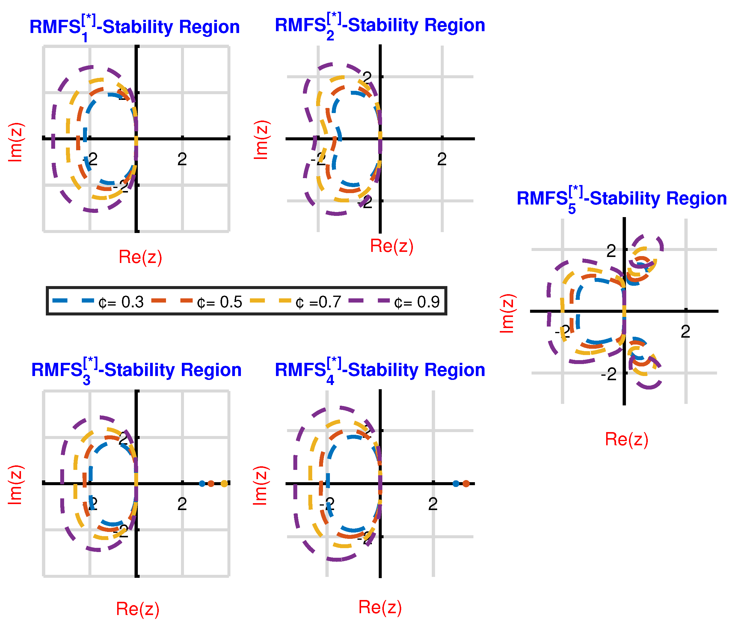
Using the CAS-MatLab computing tool, the stability region of RMFS${}_1{}^{[\ast ]}-{\mathrm{RMFS}}_5^{[\ast ]}$ is depicted for various values of ¢. The newly proposed fractional-order methods have better stability regions than the other existing fractional schemes RMFS${}_1{}^{[\ast ]}-{\mathrm{RMFS}}_2^{[\ast ]}$, as illustrated in Figure 1.

Figure 1 illustrates the stability regions of the proposed methods, while

Table 1. Stability analysis comparison of ${\mathrm{RMFS}}_1^{[\ast ]}-{\mathrm{RMFS}}_5^{[\ast ]}$.

¢	${\mathrm{RMFS}}_1^{[\ast ]}$	${\mathrm{RMFS}}_2^{[\ast ]}$	${\mathrm{RMFS}}_3^{[\ast ]}$	${\mathrm{RMFS}}_4^{[\ast ]}$	${\mathrm{RMFS}}_5^{[\ast ]}$
$0.1$	$[-1.739479,0]$	$[-1.490982,0]$	$[-1.34,-0.008]$	$[-3.12,-0.01]$	$[-1.34,-0.008]$
$0.3$	$[-2.116232,0]$	$[-1.490982,0]$	$[-1.42,-0.008]$	$[-3.71,-0.01]$	$[-1.42,-0.008]$
$0.5$	$[-1.490982,0]$	$[-1.695391,0]$	$[-1.61,-0.008]$	$[-4.20,-0.01$	$[-1.61,-0.008]$
$0.7$	$[-1.695391,0]$	$[-1.995992,0]$	$[-1.90,-0.008]$	$[-4.96,-0.01]$	$[-1.90,-0.008]$
$0.9$	$[-1.995992,0]$	$[-2.422846,0]$	$[-2.32,-0.008]$	$[-6.03,-0.01]$	$[-2.32,-0.008]$

lists the corresponding stability intervals for various fractional orders. The results show that the proposed methods have better stability and wider stability regions compared to the existing fractional-order methods.

3. Fractional Scheme Implementation and Performance Assessment

To assess the accuracy and efficiency of fractional-order methods, both fixed-step-size and variable-step-size strategies are implemented in this section.

3.1. Fixed-Step-Size Strategies

The fixed-step-size technique keeps the time step consistent throughout the integration intervals. This approach simplifies implementation and maintains consistent time resolution. Applying it to FIVPs with varying solutions could result in a loss of accuracy or efficiency. To evaluate the accuracy of the proposed methods, we use the following error formula:

$$\mathrm{Maximum}-\mathrm{Error}=\underset{j=0,1,\dots ,n}{max}∥y\left(t_j\right)-y_j∥,$$

(57)

where

• $y\left(t_j\right)$ is the exact solution;
• $y_j$ is the approximated solution by using fractional schemes at each grid point $t_j$.

It is easier to find convergence orders and perform theoretical stability analysis using fixed-step-size approaches. This formulation enables direct accuracy assessment without interpolation or resampling, which is particularly useful for comparing the methodology with other existing methods in the literature. Furthermore, fixed-step-size techniques produce predictable, reproducible results that are unaffected by floating-point fluctuations, ensuring uniform results.

3.2. Adaptive-Step-Size Strategies

The adjustable step-size methods dynamically modify the grid points to improve the performance. To ensure accuracy and effectiveness, the adjustment is predicated on local error estimation as follows:

$$Err=∥y\left(t_j\right)-y_j∥.$$

(58)

In complex simulations, it lowers computational costs and guarantees improved stability. This technique offers improved accuracy while requiring minimal computational effort. Each step involves calculating an estimated error (Err) and comparing it with a predetermined tolerance (Tol). The adaptive-step-size strategy used in this study is inspired by a similar strategy reported in [26]:

• –

  If $Err\le Tol$, the step is accepted, and the step size is increased to improve efficiency.

  –

  If $Err>Tol$, the step is rejected, and the step size is reduced to improve accuracy.

  –

  An adaptive-step-size strategy is used, with the fractional Euler method in (3) serving as a local error estimate.

The dynamic adjustment is implemented using the following strategy to improve the overall performance of the proposed methods:

$$h_{new}={\eta }^{[\ast ]}\times h_{old}{\left({\displaystyle \frac{Tol}{Err}}\right)}^{{\displaystyle \frac{1}{¢+1}}},$$

(59)

where the adjustment factor ${\eta }^{[\ast ]}\in \left(0,1\right)$ protects against step-size failures, Tol represents the predefined absolute tolerance, and ¢ indicates the order of the lower-order approach in (30). This adaptive technique ensures that errors are managed efficiently and reliably during the numerical solution process.

3.3. Implementations of RMFS${}_1{}^{[\ast ]}-{\mathit{RMFS}}_5^{[\ast ]}$

In this subsection, we describe the implementation of the proposed and existing fractional numerical methods using fixed- and adaptive-step-size strategies. Algorithms 1 and 2 provide a structured approach to solving FIVPs and enable a consistent comparison of method performance in terms of accuracy and computational effort.

Algorithm 1 (Fixed Step Size): This algorithm solves FIVPs by using a fixed step size h. The main steps are shown below.

Algorithm 1: Use of ${\mathrm{RMFS}}_3^{[\ast ]}$ to solve FIVPs with a fixed step length.
Steps	Description
1: Initialize	Define $D^{\left[\vartheta \right]}y\left(t\right)=f\left(t,y\left(t\right)\right);y^k\left({\theta }_0^{[\ast ]}\right)=y_0^k,$
	Read the initial values of ($t_0$ and $y_0$), the values of fractional
	parameter ¢, number of steps (n) and end point.
	Choose the step size $h=$($t_n-t_0$)$/n$
2: Start loop	Set $j=0$
over time
3: Compute $k_1$	$k_1=f\left(t_j,y_j\right)$
4: Compute $k_2$	$k_2=f\left(t_j+{\displaystyle \frac{2}{5}}{\displaystyle \frac{h^{¢}}{\Gamma \left(¢+1\right)}},y_j+{\displaystyle \frac{h^{¢}}{\Gamma \left(¢+1\right)}}{\displaystyle \frac{2}{5}}{k}_2\right)$
5: Update solution	$y_{j+1}=y_j+{\displaystyle \frac{h^{¢}}{\Gamma \left(¢+1\right)}}\left({\displaystyle \frac{2k_2-k_1}{2}}+{\displaystyle \frac{k_1{k}_2}{k_1+k_2}}\right)$
	$y_j=y_0.$
	$j=j+1.$
	while $j<n$ do
	Approximate solution $y_j$ at discrete time points.
6: End loop	end while

Algorithm 2 (Adaptive Step Size): This algorithm uses an adaptive-step-size strategy to control the local error during the integration process.

Algorithm 2: Use of ${\mathrm{RMFS}}_3^{[\ast ]}$ to solve FIVPs with adaptive-step-size technique.
Steps	Description
1: Initialize	Define $D^{\left[\vartheta \right]}y\left(t\right)=f\left(t,y\left(t\right)\right);y^k\left({\theta }_0^{[\ast ]}\right)=y_0^k,$
	Choose initial step size h$0$, the values of fractional parameter ¢,
	error tolerance Tol, and set $t_j=t_0$
2: Start loop over time	while $j<N$ do
3: Compute $k_1$	$k_1=f\left(t_j,y_j\right)$
4: Compute $k_2$	$k_2=f\left(t_j+{\displaystyle \frac{2}{5}}{\displaystyle \frac{h^{¢}}{\Gamma \left(¢+1\right)}},y_j+{\displaystyle \frac{h^{¢}}{\Gamma \left(¢+1\right)}}{\displaystyle \frac{2}{5}}{k}_2\right)$
5: Compute tentative	$y_{j+1}=y_j+{\displaystyle \frac{h^{¢}}{\Gamma \left(¢+1\right)}}\left({\displaystyle \frac{2k_2-k_1}{2}}+{\displaystyle \frac{k_1{k}_2}{k_1+k_2}}\right)$
solution
6: Estimate local error	Compute error error norm $Err={∥.∥}_{\infty }$
7: Adjust step size	$j=j+1.$
8: Accept or reject step	$\left\{\begin{array}{c}\mathrm{If}Err>Tol,\mathrm{reduce}\mathrm{h};\mathrm{if}\mathrm{Err}<\mathrm{Tol}/2;\mathrm{increase}\mathrm{h};\\ \mathrm{Use}:h_{new}={\eta }^{[\ast ]}\times h_{old}{\left({\displaystyle \frac{Tol}{Err}}\right)}^{{\displaystyle \frac{1}{\vartheta +1}}}.\\ \mathrm{If}Err\le Tol,\mathrm{accept}{y}_{j+1}=y_j\mathrm{and}\mathrm{update}{t}_j=t_0+h,\\ \mathrm{otherwise},\mathrm{recompute}\mathrm{with}\mathrm{new}\mathrm{h}.\end{array}\right.$
9: End loop	end while
10: Output	Approximate solution $y_j$ at adaptive time steps.

To ensure clarity and uniformity, we use the following abbreviations:

h	Step length
Exact	Exact solution
MSE$\infty$	Mean square error norm
Max-Error	Maximum error
${∥.∥}_{\infty }$	Error norm
Avg$\infty$	Average error
Fun	Total number of functions
${\mathrm{RMFS}}_1^{[\ast ]}-{\mathrm{RMFS}}_2^{[\ast ]}$	Existing methods of fractional order
${\mathrm{RMFS}}_3^{[\ast ]}-{\mathrm{RMFS}}_5^{[\ast ]}$	Newly developed methods of fractional order

3.4. Performance Assessment

This subsection presents numerical examples to assess the efficiency, stability, and consistency of the proposed fractional-order and some existing methods. The results demonstrate the accuracy, robustness, and computational efficiency of the proposed methods.

Example 1

([27]). In the first numerical example, we consider the following FIVP, which is used to effectively model complex systems with memory and hereditary features, as reported in [27]:

$$\left.\begin{array}{c}{⅁}^{[¢]}y\left(t\right)={\displaystyle \frac{40320}{\Gamma \left(9-¢\right)}}{t}^{8-¢}-{\displaystyle \frac{3\Gamma \left(5+\frac{¢}{2}\right)}{\Gamma \left(5-\frac{¢}{2}\right)}}{t}^{4-{\displaystyle \frac{¢}{2}}}+g\left(t\right),\\ y\left(0\right)=0,y^{\prime }\left(0\right)=0,t>0\end{array}\right\}$$

(60)

where

$$g\left(t\right)={\displaystyle \frac{9}{4}}\Gamma \left(¢+1\right)+{\left({\displaystyle \frac{3}{2}}{t}^{{\displaystyle \frac{¢}{2}}}-t^4\right)}^3-{\left(y\left(t\right)\right)}^{{\displaystyle \frac{3}{2}}}.$$

The exact solution of (60) is

$$y\left(t\right)=t^8-3t^{4+{\displaystyle \frac{¢}{2}}}+{\displaystyle \frac{9}{4}}{t}^{¢}$$

Table 2. Comparison of exact and approximate solutions with a step size of 0.1.

t	Exact	${\mathrm{RMFS}}_1^{[\ast ]}$	${\mathrm{RMFS}}_2^{[\ast ]}$	${\mathrm{RMFS}}_3^{[\ast ]}$	${\mathrm{RMFS}}_4^{[\ast ]}$	${\mathrm{RMFS}}_5^{[\ast ]}$
$0.0$	$0.0$	$0.0$	$0.0$	$0.0$	$0.0$	$0.0$
$0.2$	$0.0013085$	$0.0013453$	$0.0014435$	$0.0013086$	$0.0013076$	$0.0013043$
$0.4$	$0.0029592$	$0.0023445$	$0.0029886$	$0.0029556$	$0.0029874$	$0.0029765$
$0.6$	$0.0036968$	$0.0022342$	$0.0032342$	$0.0036956$	$0.0036685$	$0.0036934$
$0.8$	$0.0028626$	$0.0065326$	$0.0065322$	$0.0028645$	$0.0028645$	$0.0028676$
$1.0$	$0.0$	$0.0$	$0.0$	$0.0$	$0.0$	$0.0$

illustrates the exact and approximate solutions of (60) to five decimal places utilizing fractional schemes ${\mathrm{RMFS}}_1^{[\ast ]}-{\mathrm{RMFS}}_5^{[\ast ]}$ with fractional parameter values of 0.5 and step length of 0.1.

Table 3. Comparison of errors in fractional schemes with a step size of 0.1.

x	${\mathrm{RMFS}}_1^{[\ast ]}$	${\mathrm{RMFS}}_2^{[\ast ]}$	${\mathrm{RMFS}}_3^{[\ast ]}$	${\mathrm{RMFS}}_4^{[\ast ]}$	${\mathrm{RMFS}}_5^{[\ast ]}$
$0.0$	$0.0$	$0.0$	$0.0$	$0.0$	$0.0$
$0.2$	$4.45\times {10}^{-4}$	$1.44\times {10}^{-3}$	$0.86\times {10}^{-5}$	$0.76\times {10}^{-5}$	$0.43\times {10}^{-4}$
$0.4$	$3.44\times {10}^{-3}$	$0.79\times {10}^{-3}$	$1.56\times {10}^{-5}$	$2.45\times {10}^{-5}$	$0.63\times {10}^{-5}$
$0.6$	$1.87\times {10}^{-2}$	$1.56\times {10}^{-3}$	$9.66\times {10}^{-4}$	$0.08\times {10}^{-5}$	$0.17\times {10}^{-5}$
$0.8$	$9.54\times {10}^{-2}$	$3.87\times {10}^{-3}$	$3.06\times {10}^{-5}$	$6.45\times {10}^{-5}$	$1.10\times {10}^{-5}$
$1.0$	$0.0$	$0.0$	$0.0$	$0.0$	$0.0$

shows the error for a fixed step length of $0.1$, indicating that the newly constructed methods RMFS${}_3{}^{[\ast ]}-{\mathrm{RMFS}}_5^{[\ast ]}$ are more stable than the existing methods RMFS${}_1{}^{[\ast ]}-{\mathrm{RMFS}}_2^{[\ast ]}$.

The adaptive-step-size implementation is also applied to solve Example 1, using tolerances $ϵ={10}^{-2},{10}^{-3},$ and ${10}^{-6}$, to improve the convergence rate of fractional-order numerical schemes. The results of these numerical schemes are presented in

Table 4. Comparisons of fractional methods with an adjustable step size for solving (60).

Parameter		Tolerance $\in ={10}^{-2}$
Scheme	${∥.∥}_{\infty }$	Avg∞	MSE∞	CPU Time
${\mathrm{RMFS}}_1^{[\ast ]}$	$0.98\times {10}^{-1}$	$5.05\times {10}^{-2}$	$4.26\times {10}^{-2}$	$0.012312$
${\mathrm{RMFS}}_2^{[\ast ]}$	$0.65\times {10}^{-2}$	$9.06\times {10}^{-2}$	$8.57\times {10}^{-2}$	$0.023423$
${\mathrm{RMFS}}_3^{[\ast ]}$	$9.87\times {10}^{-2}$	$3.41\times {10}^{-2}$	$1.23\times {10}^{-3}$	$0.034242$
${\mathrm{RMFS}}_4^{[\ast ]}$	$2.34\times {10}^{-3}$	$1.87\times {10}^{-3}$	$0.65\times {10}^{-3}$	$0.006523$
${\mathrm{RMFS}}_5^{[\ast ]}$	$5.57\times {10}^{-3}$	$8.76\times {10}^{-3}$	$0.60\times {10}^{-3}$	$0.004363$
		Tolerance $\in ={10}^{-3}$
${\mathrm{RMFS}}_1^{[\ast ]}$	$0.24\times {10}^{-3}$	$9.98\times {10}^{-3}$	$0.87\times {10}^{-3}$	$0.54\times {10}^{-2}$
${\mathrm{RMFS}}_2^{[\ast ]}$	$5.03\times {10}^{-3}$	$3.66\times {10}^{-3}$	$4.02\times {10}^{-3}$	$7.65\times {10}^{-3}$
${\mathrm{RMFS}}_3^{[\ast ]}$	$3.17\times {10}^{-4}$	$7.51\times {10}^{-5}$	$0.78\times {10}^{-5}$	$6.34\times {10}^{-5}$
${\mathrm{RMFS}}_4^{[\ast ]}$	$8.37\times {10}^{-5}$	$7.72\times {10}^{-4}$	$9.96\times {10}^{-5}$	$3.56\times {10}^{-5}$
${\mathrm{RMFS}}_5^{[\ast ]}$	$0.37\times {10}^{-5}$	$8.72\times {10}^{-5}$	$0.45\times {10}^{-5}$	$0.28\times {10}^{-5}$
		Tolerance $\in ={10}^{-6}$
${\mathrm{RMFS}}_1^{[\ast ]}$	$3.24\times {10}^{-4}$	$9.98\times {10}^{-4}$	$2.19\times {10}^{-4}$	$5.75\times {10}^{-3}$
${\mathrm{RMFS}}_2^{[\ast ]}$	$7.07\times {10}^{-4}$	$5.64\times {10}^{-4}$	$1.87\times {10}^{-4}$	$7.67\times {10}^{-4}$
${\mathrm{RMFS}}_3^{[\ast ]}$	$7.17\times {10}^{-7}$	$9.51\times {10}^{-7}$	$6.71\times {10}^{-7}$	$6.77\times {10}^{-7}$
${\mathrm{RMFS}}_4^{[\ast ]}$	$0.36\times {10}^{-7}$	$5.79\times {10}^{-6}$	$2.13\times {10}^{-7}$	$1.23\times {10}^{-5}$
${\mathrm{RMFS}}_5^{[\ast ]}$	$0.44\times {10}^{-7}$	$0.02\times {10}^{-7}$	$2.15\times {10}^{-7}$	$1.92\times {10}^{-6}$

.

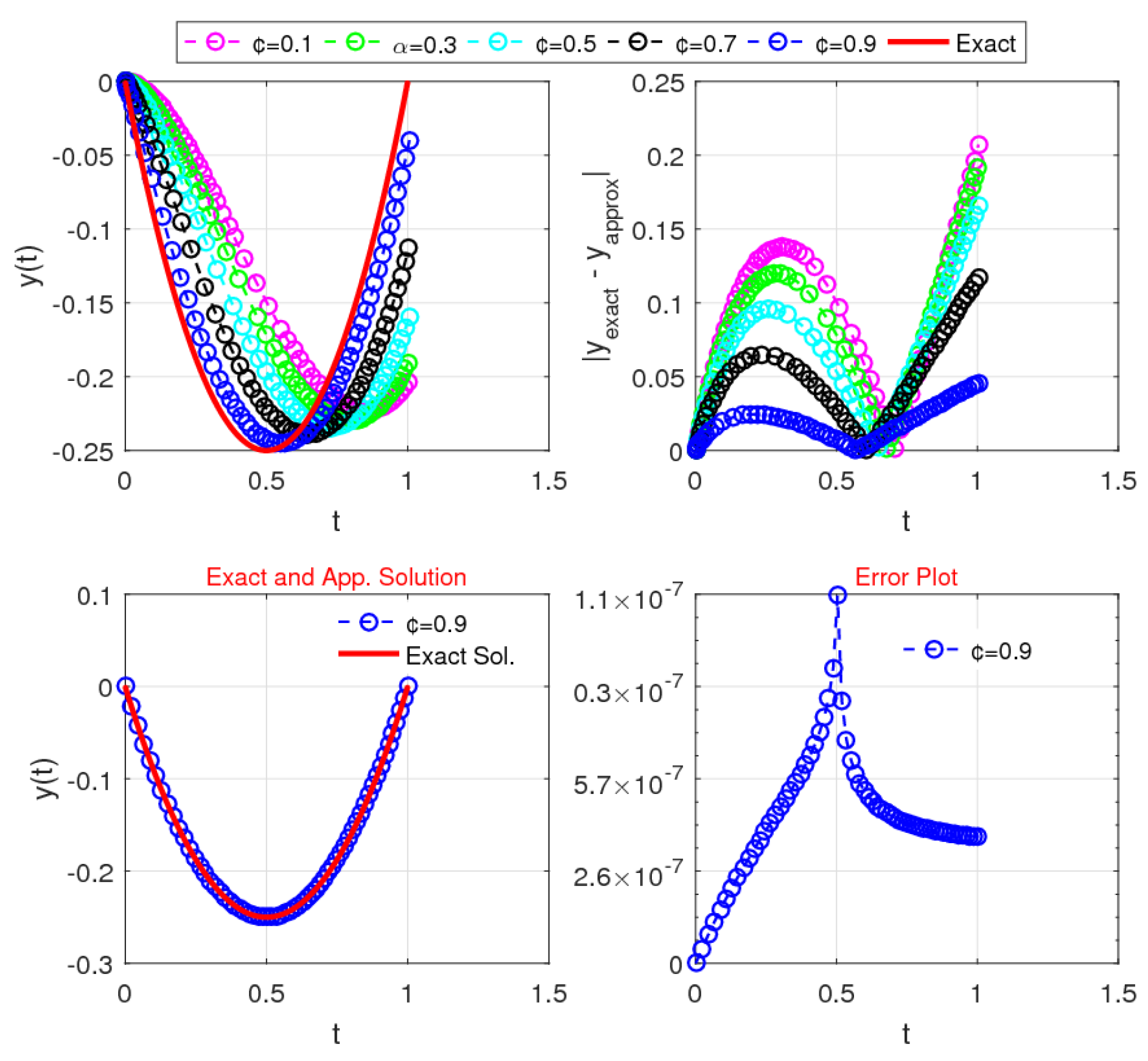
We used a variety of stopping conditions to determine the accuracy reported in Table 4, and we utilized a common tic-toc function in MATLAB R2016a to calculate the computational time in seconds. Our developed methods, RMFS${}_3{}^{[\ast ]}-{\mathrm{RMFS}}_5^{[\ast ]}$ outperform RMFS${}_1{}^{[\ast ]}-{\mathrm{RMFS}}_2^{[\ast ]}$ in terms of CPU time, MSE_∞(mean square error norm), the Avg_∞ error norm, and the ${∥.∥}_{\infty }$ error norm. Figure 2 compares exact and approximate solutions for different fractional parameter values, along with the related error plots. This figure also shows the result for $¢=0.99$, where the approximate solutions produced by RMFS${}_3{}^{[\ast ]}-{\mathrm{RMFS}}_5^{[\ast ]}$ closely match the exact solution, indicating high precision.

Example 2

([28]). Consider the fractional initial value problem as follows:

$$\left.\begin{array}{c}{⅁}^{[¢]}y\left(t\right)+y\left(t\right)={\displaystyle \frac{2}{\Gamma \left(3-¢\right)}}{t}^{2-¢}+t^2,\\ y\left(0\right)=0,t>0\end{array}\right\}$$

(61)

where $¢\in \left(0,1\right]$. The exact solution of (61) is $y\left(t\right)=t^{2¢}.$

Table 5. Comparison of exact and approximate solutions with a step size of 0.1.

t	Exact	${\mathrm{RMFS}}_1^{[\ast ]}$	${\mathrm{RMFS}}_2^{[\ast ]}$	${\mathrm{RMFS}}_3^{[\ast ]}$	${\mathrm{RMFS}}_4^{[\ast ]}$	${\mathrm{RMFS}}_5^{[\ast ]}$
$0.0$	$0.0$	$0.0$	$0.0$	$0.0$	$0.0$	$0.0$
$0.2$	$-0.16034$	$-0.16341$	$-0.16458$	$-0.160375$	$-0.165641$	$-0.160650$
$0.4$	$-0.24141$	$-0.24553$	$-0.24437$	$-0.241347$	$-0.245787$	$-0.241761$
$0.6$	$-0.24672$	$-0.24346$	$-0.24540$	$-0.246793$	$-0.246763$	$-0.246794$
$0.8$	$-0.16998$	$-0.16545$	$-0.16532$	$-0.169768$	$-0.168905$	$-0.169785$
$1.0$	$0.0$	$0.0$	$0.0$	$0.0$	$0.0$	$0.0$

illustrates the exact and approximate solutions of Example 2 utilizing fractional schemes ${\mathrm{RMFS}}_1^{[\ast ]}-{\mathrm{RMFS}}_5^{[\ast ]}$ with fractional parameter values of 0.5 and step length of 0.1.

Table 6. Comparison of errors in fractional schemes with a step size of 0.1.

x	${\mathrm{RMFS}}_1^{[\ast ]}$	${\mathrm{RMFS}}_2^{[\ast ]}$	${\mathrm{RMFS}}_3^{[\ast ]}$	${\mathrm{RMFS}}_4^{[\ast ]}$	${\mathrm{RMFS}}_5^{[\ast ]}$
$0.0$	$0.0$	$0.0$	$0.0$	$0.0$	$0.0$
$0.2$	$0.06\times {10}^{-2}$	$0.42\times {10}^{-2}$	$0.37\times {10}^{-4}$	$0.26\times {10}^{-2}$	$0.30\times {10}^{-3}$
$0.4$	$0.41\times {10}^{-2}$	$0.10\times {10}^{-2}$	$0.32\times {10}^{-3}$	$0.43\times {10}^{-2}$	$0.35\times {10}^{-3}$
$0.6$	$0.32\times {10}^{-2}$	$0.34\times {10}^{-2}$	$0.13\times {10}^{-3}$	$0.73\times {10}^{-4}$	$0.74\times {10}^{-4}$
$0.8$	$0.45\times {10}^{-2}$	$0.46\times {10}^{-2}$	$0.21\times {10}^{-3}$	$0.10\times {10}^{-3}$	$0.19\times {10}^{-3}$
$1.0$	$0.0$	$0.0$	$0.0$	$0.0$	$0.0$

shows the error for a fixed step length of 0.1, demonstrating that the newly constructed methods RMFS${}_3{}^{[\ast ]}-{\mathrm{RMFS}}_5^{[\ast ]}$ are more stable than the existing methods RMFS${}_1{}^{[\ast ]}-{\mathrm{RMFS}}_2^{[\ast ]}$.

We analyze the behavior and enhance the rate of convergence of fractional-order numerical schemes by implementing an adaptive step size using various tolerances, i.e., $\in ={10}^{-2},{10}^{-3}$, and ${10}^{-6}$.

Table 7. Comparisons of fractional methods with an adjustable step size for solving (61).

Parameter		Tolerance $\in ={10}^{-2}$
Scheme	${∥.∥}_{\infty }$	Avg∞	MSE∞	CPU Time
${\mathrm{RMFS}}_1^{[\ast ]}$	$0.36\times {10}^{-2}$	$5.01\times {10}^{-2}$	$1.87\times {10}^{-2}$	$0.0652324$
${\mathrm{RMFS}}_2^{[\ast ]}$	$0.76\times {10}^{-2}$	$7.60\times {10}^{-2}$	$2.56\times {10}^{-2}$	$0.0562623$
${\mathrm{RMFS}}_3^{[\ast ]}$	$1.23\times {10}^{-3}$	$0.06\times {10}^{-2}$	$1.67\times {10}^{-3}$	$0.0365423$
${\mathrm{RMFS}}_4^{[\ast ]}$	$0.87\times {10}^{-3}$	$1.87\times {10}^{-2}$	$4.16\times {10}^{-4}$	$0.0012532$
${\mathrm{RMFS}}_5^{[\ast ]}$	$0.55\times {10}^{-3}$	$1.19\times {10}^{-3}$	$2.14\times {10}^{-3}$	$0.0015232$
		Tolerance $\in ={10}^{-3}$
${\mathrm{RMFS}}_1^{[\ast ]}$	$9.24\times {10}^{-2}$	$4.98\times {10}^{-2}$	$2.19\times {10}^{-6}$	$5.586\times {10}^{-4}$
${\mathrm{RMFS}}_2^{[\ast ]}$	$6.76\times {10}^{-3}$	$2.08\times {10}^{-2}$	$1.53\times {10}^{-4}$	$7.758\times {10}^{-4}$
${\mathrm{RMFS}}_3^{[\ast ]}$	$1.09\times {10}^{-4}$	$1.89\times {10}^{-4}$	$6.71\times {10}^{-3}$	$6.735\times {10}^{-5}$
${\mathrm{RMFS}}_4^{[\ast ]}$	$2.37\times {10}^{-6}$	$1.98\times {10}^{-6}$	$6.01\times {10}^{-6}$	$1.324\times {10}^{-5}$
${\mathrm{RMFS}}_5^{[\ast ]}$	$0.27\times {10}^{-6}$	$1.87\times {10}^{-6}$	$2.15\times {10}^{-6}$	$1.852\times {10}^{-5}$
		Tolerance $\in ={10}^{-6}$
${\mathrm{RMFS}}_1^{[\ast ]}$	$1.24\times {10}^{-4}$	$0.12\times {10}^{-5}$	$2.09\times {10}^{-5}$	$5.565\times {10}^{-4}$
${\mathrm{RMFS}}_2^{[\ast ]}$	$6.44\times {10}^{-4}$	$4.54\times {10}^{-5}$	$1.65\times {10}^{-4}$	$7.773\times {10}^{-4}$
${\mathrm{RMFS}}_3^{[\ast ]}$	$7.17\times {10}^{-6}$	$1.51\times {10}^{-7}$	$6.98\times {10}^{-7}$	$6.755\times {10}^{-4}$
${\mathrm{RMFS}}_4^{[\ast ]}$	$7.77\times {10}^{-7}$	$1.72\times {10}^{-8}$	$0.88\times {10}^{-7}$	$1.267\times {10}^{-7}$
${\mathrm{RMFS}}_5^{[\ast ]}$	$0.39\times {10}^{-7}$	$1.72\times {10}^{-7}$	$4.56\times {10}^{-7}$	$1.256\times {10}^{-5}$

presents the results of the numerical schemes using adaptive step sizes.

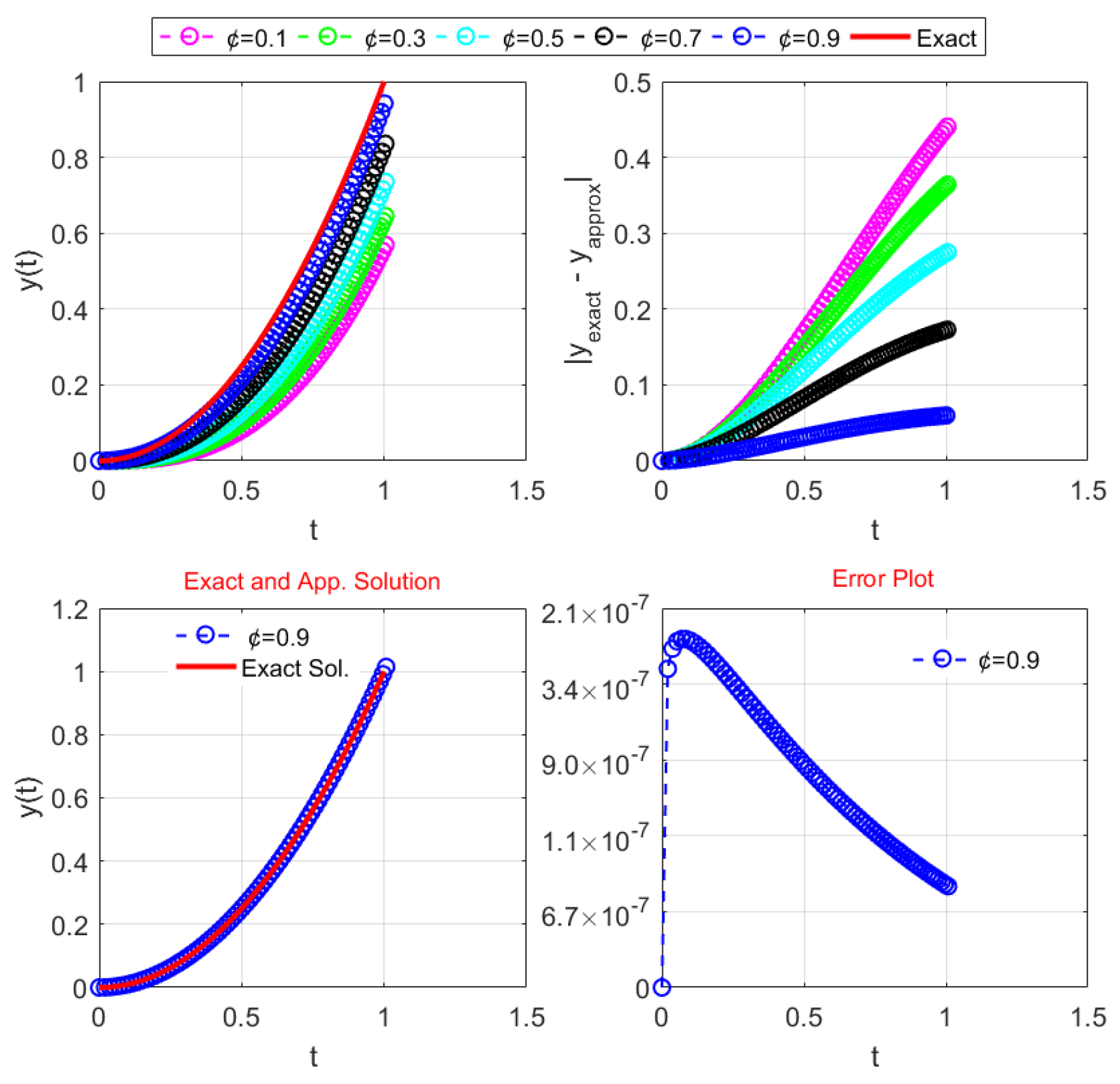
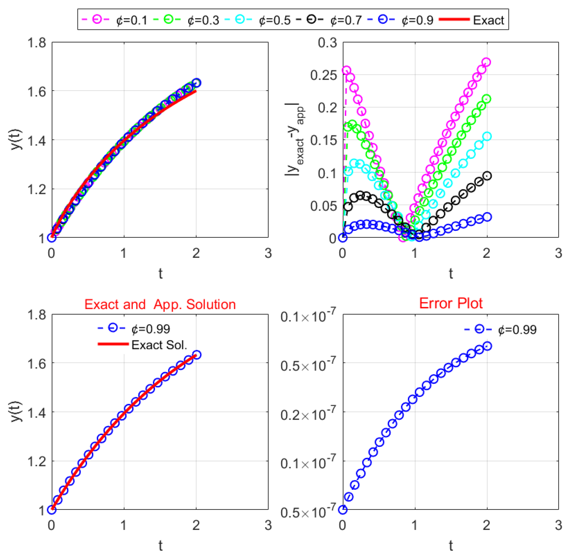
We used a variety of stopping conditions to determine the accuracy presented in Table 7, and we used a common tic-toc function before the loop in Matlab to calculate the computational time in seconds. In terms of CPU time, MSE_∞ (mean square error norm), the Avg_∞ error norm, and the ${∥.∥}_{\infty }$ error norm, our recently created methods RMFS${}_3{}^{[\ast ]}-{\mathrm{RMFS}}_5^{[\ast ]}$ perform better than the others schemes, i.e., RMFS${}_1{}^{[\ast ]}-{\mathrm{RMFS}}_2^{[\ast ]}$, as shown in Table 7. This indicates better convergence behavior and a more efficient solution for fractional differential equations. In addition, Figure 3 illustrates the associated error graph with the exact and approximate solutions for a range of fractional parameter values. Figure 3 also clearly shows that the approximate solution exactly matches the exact solution for $¢=0.99$ using RMFS${}_3{}^{[\ast ]}-{\mathrm{RMFS}}_5^{[\ast ]}$.

Example 3

([29]). Consider the fractional initial value problem as follows:

$$\left.\begin{array}{c}{⅁}^{[¢]}y\left(t\right)+y\left(t\right)={\displaystyle \frac{2}{\Gamma \left(3-¢\right)}}{t}^{2-¢}-{\displaystyle \frac{t^{1-¢}}{\Gamma \left(2-¢\right)}}+t^2-t,\\ y\left(0\right)=0,t>0\end{array}\right\}$$

(62)

where $¢\in \left(0,1\right]$. The exact solution of (62) is $y\left(t\right)=t^2-t.$

Table 8. Comparison of exact and approximate solutions with a step size of 0.1.

t	Exact	${\mathrm{RMFS}}_1^{[\ast ]}$	${\mathrm{RMFS}}_2^{[\ast ]}$	${\mathrm{RMFS}}_3^{[\ast ]}$	${\mathrm{RMFS}}_4^{[\ast ]}$	${\mathrm{RMFS}}_5^{[\ast ]}$
$0.0$	$0.0$	$0.0$	$0.0$	$0.0$	$0.0$	$0.0$
$0.2$	$0.04$	$0.04651$	$0.04613$	$0.040123$	$0.043531$	$0.040052$
$0.4$	$0.16$	$0.16346$	$0.16879$	$0.165156$	$0.160267$	$0.165654$
$0.6$	$0.36$	$0.36537$	$0.36165$	$0.360456$	$0.367195$	$0.361625$
$0.8$	$0.64$	$0.64693$	$0.64346$	$0.642421$	$0.640163$	$0.640115$
$1.0$	$1.0$	$1.02236$	$1.176$	$1.0$	$1.0$	$1.0$

illustrates the exact and approximate solution of FIVP (62) utilizing fractional schemes ${\mathrm{RMFS}}_1^{[\ast ]}-{\mathrm{RMFS}}_5^{[\ast ]}$ with fractional parameter values of 0.5 and step length of 0.1.

Table 9. Comparison of errors in fractional schemes with a step size of 0.1.

x	${\mathrm{RMFS}}_1^{[\ast ]}$	${\mathrm{RMFS}}_2^{[\ast ]}$	${\mathrm{RMFS}}_3^{[\ast ]}$	${\mathrm{RMFS}}_4^{[\ast ]}$	${\mathrm{RMFS}}_5^{[\ast ]}$
$0.0$	$0.0$	$0.0$	$0.0$	$0.0$	$0.0$
$0.2$	$2.65\times {10}^{-2}$	$4.61\times {10}^{-2}$	$1.23\times {10}^{-4}$	$0.35\times {10}^{-2}$	$0.52\times {10}^{-4}$
$0.4$	$1.34\times {10}^{-2}$	$8.79\times {10}^{-2}$	$5.15\times {10}^{-2}$	$2.63\times {10}^{-4}$	$5.65\times {10}^{-2}$
$0.6$	$1.53\times {10}^{-2}$	$1.65\times {10}^{-2}$	$0.45\times {10}^{-3}$	$7.19\times {10}^{-2}$	$0.16\times {10}^{-2}$
$0.8$	$6.93\times {10}^{-2}$	$3.46\times {10}^{-2}$	$0.42\times {10}^{-2}$	$1.63\times {10}^{-3}$	$1.15\times {10}^{-3}$
$1.0$	$2.23\times {10}^{-1}$	$1.17\times {10}^{-1}$	$0.0$	$0.0$	$0.0$

shows the error for a fixed step length of 0.1, demonstrating that the newly constructed methods RMFS${}_3{}^{[\ast ]}-{\mathrm{RMFS}}_5^{[\ast ]}$ are more stable than the existing methods RMFS${}_1{}^{[\ast ]}-{\mathrm{RMFS}}_2^{[\ast ]}$.

We analyze the behavior and enhance the rate of convergence of fractional-order numerical schemes using an adaptive-step-size strategy.

Table 10. Comparisons of fractional methods with an adjustable step size for solving (62).

Parameter		Tolerance $\in ={10}^{-2}$
Scheme	${∥.∥}_{\infty }$	Avg∞	MSE∞	CPU Time
${\mathrm{RMFS}}_1^{[\ast ]}$	$1.87\times {10}^{-1}$	$5.40\times {10}^{-2}$	$9.46\times {10}^{-2}$	$0.016545$
${\mathrm{RMFS}}_2^{[\ast ]}$	$2.65\times {10}^{-2}$	$7.98\times {10}^{-1}$	$8.57\times {10}^{-1}$	$0.027566$
${\mathrm{RMFS}}_3^{[\ast ]}$	$6.87\times {10}^{-3}$	$0.46\times {10}^{-2}$	$1.98\times {10}^{-3}$	$0.037565$
${\mathrm{RMFS}}_4^{[\ast ]}$	$2.45\times {10}^{-3}$	$8.53\times {10}^{-3}$	$8.74\times {10}^{-3}$	$0.006467$
${\mathrm{RMFS}}_5^{[\ast ]}$	$1.09\times {10}^{-3}$	$3.54\times {10}^{-3}$	$0.84\times {10}^{-3}$	$0.001656$
		Tolerance $\in ={10}^{-3}$
${\mathrm{RMFS}}_1^{[\ast ]}$	$6.24\times {10}^{-3}$	$9.98\times {10}^{-3}$	$2.19\times {10}^{-3}$	$5.55\times {10}^{-4}$
${\mathrm{RMFS}}_2^{[\ast ]}$	$6.98\times {10}^{-3}$	$4.66\times {10}^{-3}$	$1.87\times {10}^{-3}$	$7.74\times {10}^{-4}$
${\mathrm{RMFS}}_3^{[\ast ]}$	$4.45\times {10}^{-5}$	$1.51\times {10}^{-4}$	$6.45\times {10}^{-3}$	$6.75\times {10}^{-4}$
${\mathrm{RMFS}}_4^{[\ast ]}$	$6.87\times {10}^{-5}$	$1.72\times {10}^{-5}$	$4.87\times {10}^{-5}$	$1.24\times {10}^{-5}$
${\mathrm{RMFS}}_5^{[\ast ]}$	$3.23\times {10}^{-5}$	$1.72\times {10}^{-5}$	$2.45\times {10}^{-5}$	$1.53\times {10}^{-6}$
		Tolerance $\in ={10}^{-6}$
${\mathrm{RMFS}}_1^{[\ast ]}$	$1.24\times {10}^{-4}$	$9.98\times {10}^{-5}$	$2.19\times {10}^{-5}$	$5.54\times {10}^{-4}$
${\mathrm{RMFS}}_2^{[\ast ]}$	$6.03\times {10}^{-5}$	$4.66\times {10}^{-5}$	$1.87\times {10}^{-5}$	$7.37\times {10}^{-4}$
${\mathrm{RMFS}}_3^{[\ast ]}$	$0.17\times {10}^{-8}$	$1.51\times {10}^{-7}$	$6.71\times {10}^{-8}$	$6.76\times {10}^{-4}$
${\mathrm{RMFS}}_4^{[\ast ]}$	$0.37\times {10}^{-7}$	$1.72\times {10}^{-8}$	$2.15\times {10}^{-8}$	$1.72\times {10}^{-5}$
${\mathrm{RMFS}}_5^{[\ast ]}$	$0.37\times {10}^{-8}$	$1.72\times {10}^{-8}$	$2.15\times {10}^{-8}$	$8.52\times {10}^{-5}$

presents the results of the numerical schemes.

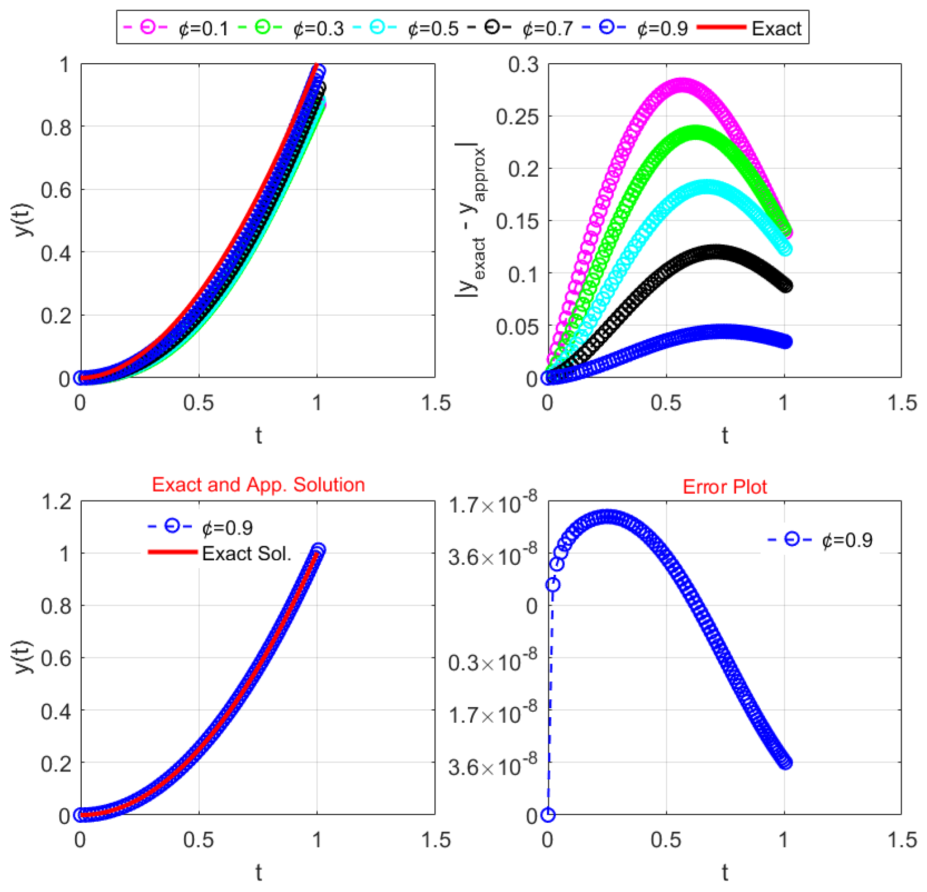
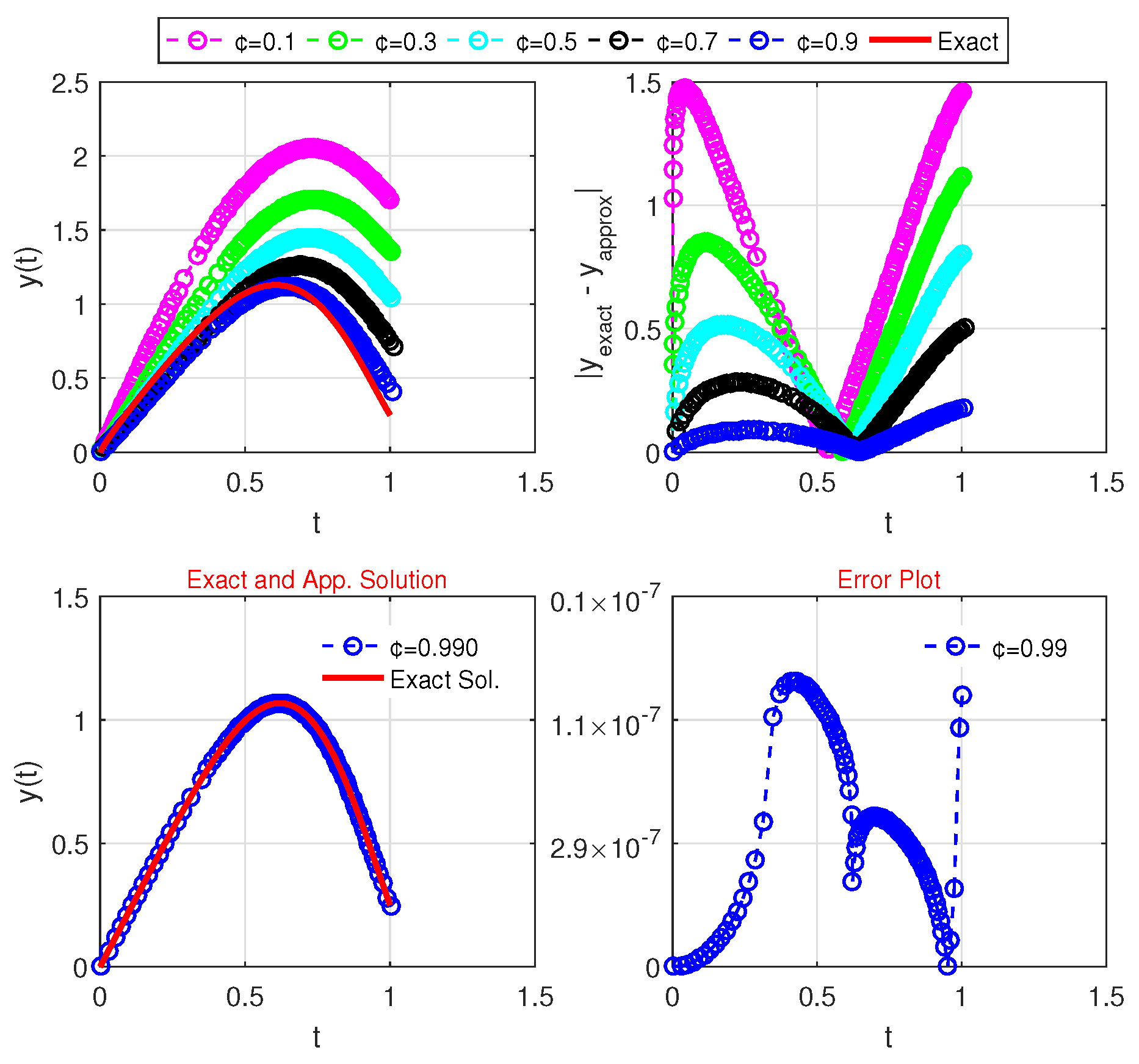
We used a variety of stopping conditions to determine the accuracy reported in Table 10, and we used a common tic-toc function before the loop in Matlab to calculate the computational time in seconds. In terms of CPU time, MSE_∞ (mean square error norm), the Avg_∞ error norm, and the ${∥.∥}_{\infty }$ error norm, our developed methods RMFS${}_3{}^{[\ast ]}-{\mathrm{RMFS}}_5^{[\ast ]}$ perform better than the other schemes, i.e., RMFS${}_1{}^{[\ast ]}-{\mathrm{RMFS}}_2^{[\ast ]}$, as indicated in Table 10. Figure 4 also compares the exact and approximate solutions for various fractional parameter values, as well as the corresponding error graph. Figure 4 also clearly shows that the approximate solution exactly matches the exact solution for $¢=0.99$ using RMFS${}_3{}^{[\ast ]}-{\mathrm{RMFS}}_5^{[\ast ]}$.

Example 4

([30]). Consider the fractional initial value problem as follows:

$$\left.\begin{array}{c}{⅁}^{[¢]}y\left(t\right)+2{\left(y\left(t\right)\right)}^2=\Gamma \left(¢+2\right)t+2{\left(t^{¢+1}\right)}^2,\\ y\left(0\right)=0,t>0\end{array}\right\}$$

(63)

where $¢\in \left(0,1\right]$. The exact solution of (63) is $y\left(t\right)=t^{+1}.$

Table 11. Comparison of exact and approximate solutions with a step size of 0.1.

t	Exact	${\mathrm{RMFS}}_1^{[\ast ]}$	${\mathrm{RMFS}}_2^{[\ast ]}$	${\mathrm{RMFS}}_3^{[\ast ]}$	${\mathrm{RMFS}}_4^{[\ast ]}$	${\mathrm{RMFS}}_5^{[\ast ]}$
$0.0$	$0.0$	$0.0$	$0.0$	$0.0$	$0.0$	$0.0$
$0.2$	$0.04064$	$0.04066$	$0.04064$	$0.04067$	$0.04062$	$0.04068$
$0.4$	$0.16147$	$0.16176$	$0.16734$	$0.16145$	$0.16147$	$0.16187$
$0.6$	$0.36184$	$0.36309$	$0.36687$	$0.36134$	$0.36184$	$0.36184$
$0.8$	$0.64143$	$0.64567$	$0.64578$	$0.64176$	$0.64143$	$0.64143$
$1.0$	$1.0$	$1.0$	$1.0$	$1.0$	$1.0$	$1.0$

illustrates the exact and approximate solutions of Example 4 utilizing fractional schemes ${\mathrm{RMFS}}_1^{[\ast ]}-{\mathrm{RMFS}}_5^{[\ast ]}$ with fractional parameter values of 0.5 and step length of 0.1.

Table 12. Comparison of errors in fractional schemes with a step size of 0.1.

x	${\mathrm{RMFS}}_1^{[\ast ]}$	${\mathrm{RMFS}}_2^{[\ast ]}$	${\mathrm{RMFS}}_3^{[\ast ]}$	${\mathrm{RMFS}}_4^{[\ast ]}$	${\mathrm{RMFS}}_5^{[\ast ]}$
$0.0$	$0.0$	$0.0$	$0.0$	$0.0$	$0.0$
$0.2$	$2.04\times {10}^{-4}$	$3.87\times {10}^{-3}$	$1.87\times {10}^{-4}$	$4.87\times {10}^{-4}$	$4.55\times {10}^{-4}$
$0.4$	$3.06\times {10}^{-4}$	$8.34\times {10}^{-2}$	$7.46\times {10}^{-5}$	$8.34\times {10}^{-5}$	$7.34\times {10}^{-3}$
$0.6$	$6.53\times {10}^{-2}$	$1.09\times {10}^{-2}$	$3.87\times {10}^{-3}$	$3.64\times {10}^{-4}$	$5.87\times {10}^{-5}$
$0.8$	$7.34\times {10}^{-2}$	$5.98\times {10}^{-2}$	$0.45\times {10}^{-5}$	$8.44\times {10}^{-3}$	$8.34\times {10}^{-3}$
$1.0$	$0.0$	$0.0$	$0.0$	$0.0$	$0.0$

shows the error for a fixed step length of 0.1, indicating that the newly constructed methods RMFS${}_3{}^{[\ast ]}-{\mathrm{RMFS}}_5^{[\ast ]}$ are more stable than the existing methods RMFS${}_1{}^{[\ast ]}-{\mathrm{RMFS}}_2^{[\ast ]}$. We analyze the behavior and enhance the rate of convergence of fractional-order numerical schemes using the adaptive-step-size approach with various tolerances, i.e., $\in ={10}^{-2},{10}^{-3}$, and ${10}^{-6}$.

Table 13. Comparisons of fractional methods with an adjustable step size for solving (63).

Parameter		Tolerance $\in ={10}^{-2}$
Scheme	${∥.∥}_{\infty }$	Avg∞	MSE∞	CPU Time
${\mathrm{RMFS}}_1^{[\ast ]}$	$1.36\times {10}^{-2}$	$5.05\times {10}^{-1}$	$7.96\times {10}^{-1}$	$5.578\times {10}^{-2}$
${\mathrm{RMFS}}_2^{[\ast ]}$	$9.61\times {10}^{-1}$	$7.76\times {10}^{-2}$	$8.56\times {10}^{-1}$	$5.764\times {10}^{-2}$
${\mathrm{RMFS}}_3^{[\ast ]}$	$1.76\times {10}^{-3}$	$9.29\times {10}^{-3}$	$1.94\times {10}^{-3}$	$6.385\times {10}^{-4}$
${\mathrm{RMFS}}_4^{[\ast ]}$	$6.91\times {10}^{-4}$	$1.76\times {10}^{-3}$	$0.01\times {10}^{-3}$	$8.394\times {10}^{-4}$
${\mathrm{RMFS}}_5^{[\ast ]}$	$4.67\times {10}^{-4}$	$0.14\times {10}^{-3}$	$2.65\times {10}^{-4}$	$6.539\times {10}^{-3}$
		Tolerance $\in ={10}^{-3}$
${\mathrm{RMFS}}_1^{[\ast ]}$	$1.24\times {10}^{-3}$	$9.34\times {10}^{-3}$	$2.19\times {10}^{-3}$	$5.346\times {10}^{-3}$
${\mathrm{RMFS}}_2^{[\ast ]}$	$6.03\times {10}^{-4}$	$1.98\times {10}^{-3}$	$1.07\times {10}^{-3}$	$7.791\times {10}^{-3}$
${\mathrm{RMFS}}_3^{[\ast ]}$	$3.76\times {10}^{-6}$	$1.35\times {10}^{-5}$	$6.98\times {10}^{-3}$	$6.782\times {10}^{-4}$
${\mathrm{RMFS}}_4^{[\ast ]}$	$5.87\times {10}^{-5}$	$1.87\times {10}^{-5}$	$4.76\times {10}^{-5}$	$1.990\times {10}^{-5}$
${\mathrm{RMFS}}_5^{[\ast ]}$	$4.98\times {10}^{-6}$	$1.98\times {10}^{-6}$	$8.15\times {10}^{-6}$	$1.285\times {10}^{-6}$
		Tolerance $\in ={10}^{-6}$
${\mathrm{RMFS}}_1^{[\ast ]}$	$1.24\times {10}^{-4}$	$9.98\times {10}^{-4}$	$2.19\times {10}^{-4}$	$5.576\times {10}^{-5}$
${\mathrm{RMFS}}_2^{[\ast ]}$	$6.03\times {10}^{-5}$	$4.66\times {10}^{-5}$	$1.87\times {10}^{-4}$	$7.735\times {10}^{-4}$
${\mathrm{RMFS}}_3^{[\ast ]}$	$0.17\times {10}^{-7}$	$1.51\times {10}^{-7}$	$6.71\times {10}^{-6}$	$6.711\times {10}^{-7}$
${\mathrm{RMFS}}_4^{[\ast ]}$	$0.37\times {10}^{-7}$	$1.72\times {10}^{-7}$	$2.15\times {10}^{-7}$	$1.208\times {10}^{-8}$
${\mathrm{RMFS}}_5^{[\ast ]}$	$0.37\times {10}^{-7}$	$1.72\times {10}^{-7}$	$2.15\times {10}^{-7}$	$1.209\times {10}^{-7}$

reports the results of the numerical schemes.

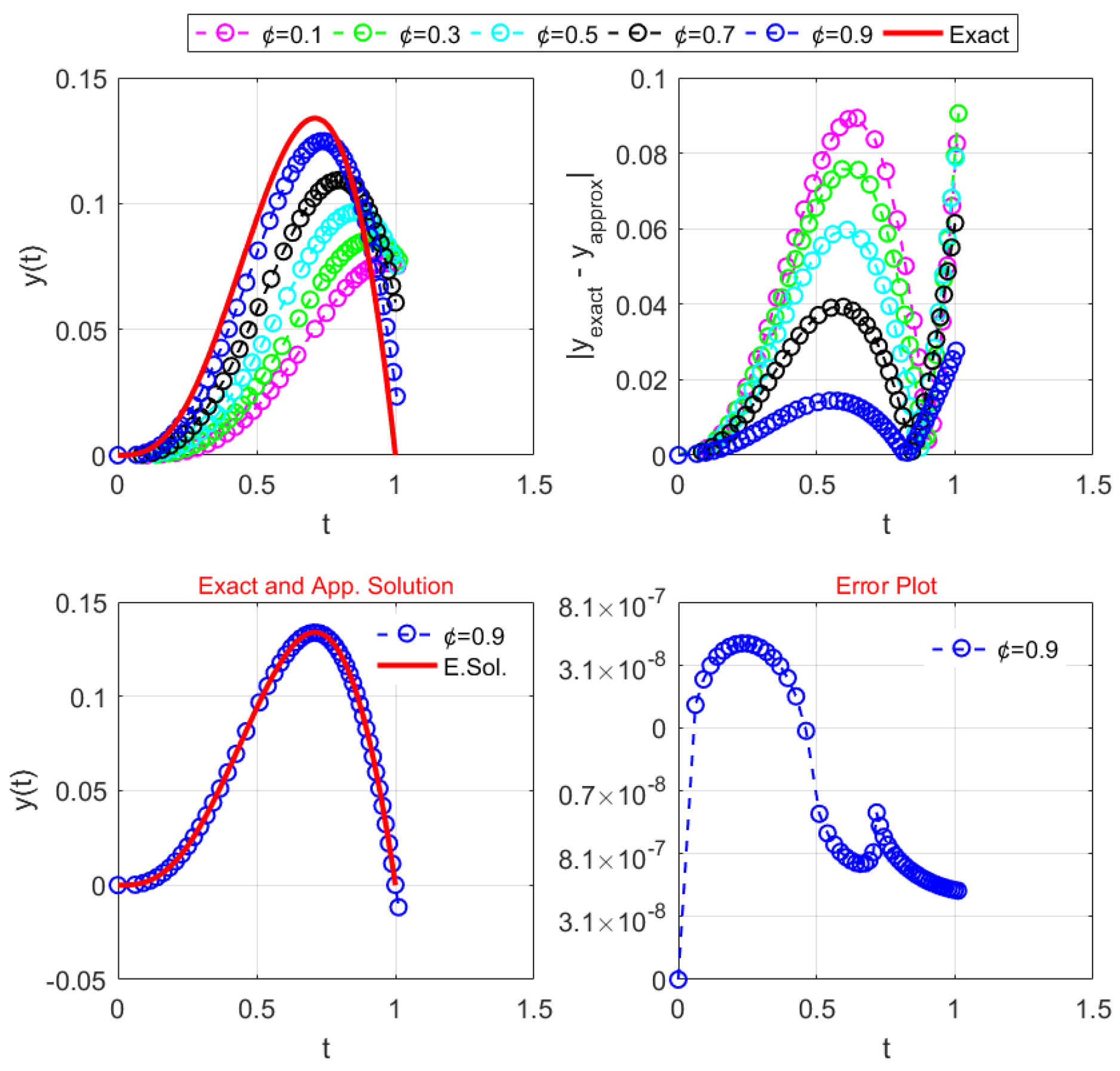
We used a variety of stopping conditions to determine the accuracy presented in Table 13, and we used a common tic-toc function before the loop in Matlab to calculate the computational time in seconds. Our recently developed methods RMFS${}_3{}^{[\ast ]}-{\mathrm{RMFS}}_5^{[\ast ]}$ outperform other schemes, i.e., RMFS${}_1{}^{[\ast ]}-{\mathrm{RMFS}}_2^{[\ast ]}$, in terms of CPU time, MSE_∞ (mean square error norm), the Avg_∞ error norm, and the ${∥.∥}_{\infty }$ error norm, as illustrated in Table 13. Figure 5 also compares the exact and approximate solutions for various fractional parameter values, as well as the corresponding error graph. Figure 5 also clearly shows that the approximate solution exactly matches the exact solution for $¢=0.99$ using RMFS${}_3{}^{[\ast ]}-{\mathrm{RMFS}}_5^{[\ast ]}$.

Example 5

([31]). Consider the fractional initial value problem as follows:

$$\left.\begin{array}{c}{⅁}^{[¢]}y\left(t\right)+y^2\left(t\right)=g\left(t\right),\\ y\left(0\right)=0,y^{\prime }\left(0\right)=0,t>0\end{array}\right\}$$

(64)

where

$$g\left(t\right)={\displaystyle \frac{\Gamma \left(6\right)}{\Gamma \left(6-¢\right)}}{t}^{5-¢}-{\displaystyle \frac{3\Gamma \left(5\right)}{\Gamma \left(5-¢\right)}}{t}^{4-¢}+{\displaystyle \frac{2\Gamma \left(4\right)}{\Gamma \left(4-¢\right)}}{t}^{3-¢}+{\left(t^5-3t^4+2t^3\right)}^2$$

and $¢\in \left(0,1\right]$. The exact solution of (64) is

$$y\left(t\right)=t^5-3t^4+2t^3.$$

Table 14. Comparison of exact and approximate solutions with a step size of 0.1.

t	Exact	${\mathrm{RMFS}}_1^{[\ast ]}$	${\mathrm{RMFS}}_2^{[\ast ]}$	${\mathrm{RMFS}}_3^{[\ast ]}$	${\mathrm{RMFS}}_4^{[\ast ]}$	${\mathrm{RMFS}}_5^{[\ast ]}$
$0.0$	$0.0$	$0.0$	$0.0$	$0.0$	$0.0$	$0.0$
$0.2$	$0.01152$	$0.01198$	$0.01365$	$0.011342$	$0.011654$	$0.0115276$
$0.4$	$0.06144$	$0.06146$	$0.06176$	$0.061443$	$0.061443$	$0.0614445$
$0.6$	$0.12096$	$0.12096$	$0.12186$	$0.120965$	$0.120966$	$0.1209635$
$0.8$	$0.12288$	$0.12287$	$0.12334$	$0.122838$	$0.122883$	$0.1228864$
$1.0$	$0.0$	$0.0$	$0.0$	$0.0$	$0.0$	$0.0$

illustrates the exact and approximate solutions for Example 5 utilizing fractional schemes ${\mathrm{RMFS}}_1^{[\ast ]}-{\mathrm{RMFS}}_5^{[\ast ]}$ with fractional parameter values of 0.5 and step length of 0.1.

Table 15. Comparison of errors in fractional schemes with a step size of 0.1.

x	${\mathrm{RMFS}}_1^{[\ast ]}$	${\mathrm{RMFS}}_2^{[\ast ]}$	${\mathrm{RMFS}}_3^{[\ast ]}$	${\mathrm{RMFS}}_4^{[\ast ]}$	${\mathrm{RMFS}}_5^{[\ast ]}$
$0.0$	$0.0$	$0.0$	$0.0$	$0.0$	$0.0$
$0.2$	$2.87\times {10}^{-3}$	$9.65\times {10}^{-2}$	$6.09\times {10}^{-4}$	$9.59\times {10}^{-4}$	$1.55\times {10}^{-4}$
$0.4$	$1.54\times {10}^{-3}$	$5.75\times {10}^{-3}$	$1.96\times {10}^{-5}$	$2.62\times {10}^{-4}$	$0.60\times {10}^{-4}$
$0.6$	$0.98\times {10}^{-3}$	$0.87\times {10}^{-2}$	$9.28\times {10}^{-3}$	$6.14\times {10}^{-5}$	$5.45\times {10}^{-5}$
$0.8$	$7.78\times {10}^{-3}$	$3.45\times {10}^{-2}$	$0.06\times {10}^{-5}$	$7.17\times {10}^{-3}$	$6.43\times {10}^{-3}$
$1.0$	$0.0$	$0.0$	$0.0$	$0.0$	$0.0$

shows the error for a fixed step length of 0.1, indicating that the newly constructed methods RMFS${}_3{}^{[\ast ]}-{\mathrm{RMFS}}_5^{[\ast ]}$ are more stable than the existing methods RMFS${}_1{}^{[\ast ]}-{\mathrm{RMFS}}_2^{[\ast ]}$.

Table 16. Comparisons of fractional methods with an adjustable step size for solving (64).

Parameter		Tolerance $\in ={10}^{-2}$
Scheme	${∥.∥}_{\infty }$	Avg∞	MSE∞	CPU Time
${\mathrm{RMFS}}_1^{[\ast ]}$	$1.36\times {10}^{-2}$	$5.05\times {10}^{-2}$	$9.96\times {10}^{-2}$	$0.0657124$
${\mathrm{RMFS}}_2^{[\ast ]}$	$9.65\times {10}^{-2}$	$7.66\times {10}^{-2}$	$8.56\times {10}^{-1}$	$0.0875723$
${\mathrm{RMFS}}_3^{[\ast ]}$	$1.05\times {10}^{-3}$	$9.56\times {10}^{-2}$	$1.64\times {10}^{-2}$	$0.0376542$
${\mathrm{RMFS}}_4^{[\ast ]}$	$0.61\times {10}^{-3}$	$1.05\times {10}^{-3}$	$0.12\times {10}^{-3}$	$0.0067645$
${\mathrm{RMFS}}_5^{[\ast ]}$	$6.71\times {10}^{-3}$	$0.17\times {10}^{-3}$	$2.15\times {10}^{-3}$	$6.7\times {10}^{-4}$
		Tolerance $\in ={10}^{-3}$
${\mathrm{RMFS}}_1^{[\ast ]}$	$1.24\times {10}^{-3}$	$9.98\times {10}^{-3}$	$2.19\times {10}^{-3}$	$5.095\times {10}^{-4}$
${\mathrm{RMFS}}_2^{[\ast ]}$	$6.03\times {10}^{-4}$	$4.87\times {10}^{-5}$	$1.87\times {10}^{-4}$	$7.677\times {10}^{-4}$
${\mathrm{RMFS}}_3^{[\ast ]}$	$0.17\times {10}^{-5}$	$1.51\times {10}^{-4}$	$6.71\times {10}^{-4}$	$6.867\times {10}^{-4}$
${\mathrm{RMFS}}_4^{[\ast ]}$	$0.19\times {10}^{-5}$	$1.75\times {10}^{-5}$	$0.60\times {10}^{-5}$	$1.082\times {10}^{-5}$
${\mathrm{RMFS}}_5^{[\ast ]}$	$0.67\times {10}^{-5}$	$1.72\times {10}^{-5}$	$1.05\times {10}^{-5}$	$1.209\times {10}^{-5}$
		Tolerance $\in ={10}^{-6}$
${\mathrm{RMFS}}_1^{[\ast ]}$	$1.23\times {10}^{-5}$	$9.98\times {10}^{-5}$	$2.19\times {10}^{-5}$	$1.809\times {10}^{-4}$
${\mathrm{RMFS}}_2^{[\ast ]}$	$6.83\times {10}^{-5}$	$4.65\times {10}^{-5}$	$1.87\times {10}^{-5}$	$7.744\times {10}^{-4}$
${\mathrm{RMFS}}_3^{[\ast ]}$	$4.15\times {10}^{-7}$	$1.51\times {10}^{-7}$	$6.71\times {10}^{-6}$	$6.376\times {10}^{-4}$
${\mathrm{RMFS}}_4^{[\ast ]}$	$9.37\times {10}^{-7}$	$1.02\times {10}^{-7}$	$7.05\times {10}^{-8}$	$1.276\times {10}^{-5}$
${\mathrm{RMFS}}_5^{[\ast ]}$	$7.87\times {10}^{-8}$	$0.99\times {10}^{-8}$	$0.18\times {10}^{-8}$	$0.246\times {10}^{-6}$

presents the results of the numerical schemes with adaptive step size.

We employed a variety of stopping conditions to determine the accuracy reported in Table 16, and we utilized a common tic-toc function in MATLAB to compute the processing time in seconds. Our developed methods, RMFS${}_3{}^{[\ast ]}-{\mathrm{RMFS}}_5^{[\ast ]}$, outperform other schemes, including RMFS${}_1{}^{[\ast ]}-{\mathrm{RMFS}}_2^{[\ast ]}$, in terms of CPU time, MSE_∞ (mean square error norm), the Avg_∞ error norm, and the ${∥.∥}_{\infty }$ error norm, as shown in Table 16. Figure 6 compares the exact and numerical solutions for different ¢ values, along with the related error plots. For $¢=0.99$, the approximate solutions produced by RMFS${}_3{}^{[\ast ]}-{\mathrm{RMFS}}_5^{[\ast ]}$ closely match the exact solution, indicating high precision of the proposed method.

Example 6

(Forced Fractional Relaxation). This model is a forced fractional relaxation system characterized by the Caputo fractional IVP [32], which is useful for describing dynamical processes in which memory and heredity effects cannot be ignored. The fractional relaxation system, which integrates prior states through the fractional derivative of order α, provides a more accurate description of complicated materials and processes compared with the classical relaxation model, which only considers the current state. This is especially relevant in viscoelasticity, dielectric relaxation, anomalous diffusion, and biomedical engineering, where experimental results frequently reveal power-law decays rather than simple exponential ones. In physiological models, the forcing term $Qg\left(t\right)$ refers to an external input, such as stress, field, or metabolic stimulation. Long-term memory dynamics and non-exponential relaxation are naturally captured by the Mittag-Leffler function, a fractional counterpart of the exponential function utilized in the model’s solution. The given model can be described by the Caputo fractional initial value problem

$$\left.\begin{array}{c}{⅁}^{[¢]}y\left(t\right)=-\kappa y\left(t\right)+Qg\left(t\right),\\ y\left(0\right)=y_0,\end{array}\right\}$$

(65)

where the parameters are $\kappa >0$ (relaxation rate), $Q\in \mathbb{R}$ (force amplitude), $\mu >-1$ (force exponent), $g\left(t\right)=t^{\mu }$, and $¢\in \left(0,1\right].$ The exact solution of (65) is

$$y\left(t\right)=y_0{E}_{¢}\left(-\kappa t^{¢}\right)+Q{t}^{¢+\mu }{E}_{¢,¢+\mu +1}\left(-\kappa t^{¢}\right),$$

(66)

where $E_{¢}(-\kappa t^{¢})$ and $E_{¢,¢+\mu +1}(-\kappa t^{¢})$ are the one- and two-parameter Mittag–Leffler functions, defined by (see [33])

$$E_{¢}\left(z\right)=\sum _{n=0}^{\infty }{\displaystyle \frac{z^n}{\Gamma (¢n+1)}},E_{¢,\beta }\left(z\right)=\sum _{n=0}^{\infty }{\displaystyle \frac{z^n}{\Gamma (¢n+\beta )}}.$$

In particular,

$$E_{¢}\left(-\kappa t^{¢}\right)=\sum _{n=0}^{\infty }{\displaystyle \frac{{(-\kappa t^{¢})}^n}{\Gamma (¢n+1)}},E_{¢,¢+\mu +1}\left(-\kappa t^{¢}\right)=\sum _{n=0}^{\infty }{\displaystyle \frac{{(-\kappa t^{¢})}^n}{\Gamma (¢n+¢+\mu +1)}}.$$

To simulate the model using fractional schemes, the following parameter values in (65) are given:

• $¢\in \left(0,1\right]$ is the fractional order, controlling the "memory effect" of the process.
• $\kappa =0.5$ is the relaxation rate, representing how quickly the system returns to equilibrium.
• $Q=1.0$ and $\mu =0$ specify constant external forcing.
• $y_0=1$ is the initial state.

The term

$$f(t,y)=-\kappa y\left(t\right)+Qg\left(t\right)$$

(67)

contains two competing effects: a decay term, $\kappa y\left(t\right)$, which pulls the system down, and a forcing term, $Qg\left(t\right)$, which injects energy into the system.

Table 17. Comparison of exact and approximate solutions with a step size of 0.1.

t	Exact	${\mathrm{RMFS}}_1^{[\ast ]}$	${\mathrm{RMFS}}_2^{[\ast ]}$	${\mathrm{RMFS}}_3^{[\ast ]}$	${\mathrm{RMFS}}_4^{[\ast ]}$	${\mathrm{RMFS}}_5^{[\ast ]}$
$0.0$	$0.0$	$0.0$	$0.0$	$0.0$	$0.0$	$0.0$
$0.4$	$0.18334$	$0.18367$	$0.18775$	$0.18337$	$0.18335$	$0.18334$
$0.8$	$1.33086$	$1.33054$	$1.33576$	$1.33089$	$1.33086$	$1.33086$
$1.2$	$1.14509$	$1.14578$	$1.14376$	$1.14509$	$1.14505$	$1.14509$
$1.6$	$1.54889$	$1.54809$	$1.54986$	$1.54881$	$1.54886$	$1.54889$
$2.0$	$1.62897$	$1.62842$	$1.62976$	$1.62897$	$1.62897$	$1.62897$

illustrates the exact and approximate solutions for Example 6 utilizing fractional schemes ${\mathrm{RMFS}}_1^{[\ast ]}-{\mathrm{RMFS}}_5^{[\ast ]}$ with fractional parameter values of 0.5 and step length of 0.1.

Table 17 shows the error for a fixed step length of 0.1, indicating that the newly constructed methods RMFS${}_3{}^{[\ast ]}-{\mathrm{RMFS}}_5^{[\ast ]}$ are more stable than the existing methods RMFS${}_1{}^{[\ast ]}-{\mathrm{RMFS}}_2^{[\ast ]}$.

Table 18. Comparison of errors in fractional schemes with a step size of 0.1.

x	${\mathrm{RMFS}}_1^{[\ast ]}$	${\mathrm{RMFS}}_2^{[\ast ]}$	${\mathrm{RMFS}}_3^{[\ast ]}$	${\mathrm{RMFS}}_4^{[\ast ]}$	${\mathrm{RMFS}}_5^{[\ast ]}$
$0.0$	$0.0$	$0.0$	$0.0$	$0.0$	$0.0$
$0.4$	$0.07\times {10}^{-3}$	$1.17\times {10}^{-2}$	$1.56\times {10}^{-4}$	$0.09\times {10}^{-5}$	$5.87\times {10}^{-5}$
$0.8$	$2.10\times {10}^{-3}$	$1.49\times {10}^{-2}$	$0.78\times {10}^{-4}$	$1.76\times {10}^{-5}$	$9.01\times {10}^{-6}$
$1.2$	$0.14\times {10}^{-3}$	$4.07\times {10}^{-2}$	$0.28\times {10}^{-3}$	$0.13\times {10}^{-3}$	$0.75\times {10}^{-5}$
$1.6$	$1.08\times {10}^{-3}$	$6.83\times {10}^{-2}$	$0.43\times {10}^{-5}$	$9.84\times {10}^{-3}$	$1.03\times {10}^{-5}$
$2.0$	$2.08\times {10}^{-2}$	$1.37\times {10}^{-2}$	$0.0$	$0.0$	$0.0$

presents the results of the numerical schemes with adaptive step size.

In

Table 19. Comparisons of fractional methods with an adjustable step size for solving (65).

Parameter		Tolerance $\in ={10}^{-2}$
Scheme	${∥.∥}_{\infty }$	Avg∞	MSE∞	CPU Time
${\mathrm{RMFS}}_1^{[\ast ]}$	$1.01\times {10}^{-2}$	$6.12\times {10}^{-2}$	$0.13\times {10}^{-2}$	$0.0257$
${\mathrm{RMFS}}_2^{[\ast ]}$	$3.72\times {10}^{-2}$	$1.75\times {10}^{-2}$	$1.21\times {10}^{-1}$	$0.0573$
${\mathrm{RMFS}}_3^{[\ast ]}$	$7.14\times {10}^{-3}$	$0.06\times {10}^{-2}$	$5.13\times {10}^{-2}$	$0.0376$
${\mathrm{RMFS}}_4^{[\ast ]}$	$5.32\times {10}^{-3}$	$1.78\times {10}^{-3}$	$1.87\times {10}^{-3}$	$0.0064$
${\mathrm{RMFS}}_5^{[\ast ]}$	$0.97\times {10}^{-3}$	$9.21\times {10}^{-3}$	$1.10\times {10}^{-3}$	$0.0057$
		Tolerance $\in ={10}^{-3}$
${\mathrm{RMFS}}_1^{[\ast ]}$	$8.01\times {10}^{-3}$	$0.08\times {10}^{-3}$	$2.17\times {10}^{-3}$	$1.032\times {10}^{-4}$
${\mathrm{RMFS}}_2^{[\ast ]}$	$7.01\times {10}^{-4}$	$2.13\times {10}^{-5}$	$1.01\times {10}^{-4}$	$1.607\times {10}^{-4}$
${\mathrm{RMFS}}_3^{[\ast ]}$	$9.93\times {10}^{-5}$	$6.47\times {10}^{-4}$	$6.15\times {10}^{-4}$	$0.834\times {10}^{-3}$
${\mathrm{RMFS}}_4^{[\ast ]}$	$0.58\times {10}^{-5}$	$0.51\times {10}^{-5}$	$7.32\times {10}^{-5}$	$1.202\times {10}^{-3}$
${\mathrm{RMFS}}_5^{[\ast ]}$	$0.30\times {10}^{-5}$	$4.31\times {10}^{-5}$	$9.01\times {10}^{-5}$	$1.652\times {10}^{-4}$
		Tolerance $\in ={10}^{-6}$
${\mathrm{RMFS}}_1^{[\ast ]}$	$3.03\times {10}^{-5}$	$1.78\times {10}^{-5}$	$3.09\times {10}^{-5}$	$0.443\times {10}^{-4}$
${\mathrm{RMFS}}_2^{[\ast ]}$	$1.98\times {10}^{-5}$	$0.35\times {10}^{-5}$	$6.89\times {10}^{-5}$	$3.105\times {10}^{-5}$
${\mathrm{RMFS}}_3^{[\ast ]}$	$0.05\times {10}^{-7}$	$0.11\times {10}^{-7}$	$0.01\times {10}^{-6}$	$2.001\times {10}^{-6}$
${\mathrm{RMFS}}_4^{[\ast ]}$	$1.31\times {10}^{-7}$	$3.72\times {10}^{-7}$	$1.07\times {10}^{-8}$	$7.332\times {10}^{-5}$
${\mathrm{RMFS}}_5^{[\ast ]}$	$6.56\times {10}^{-8}$	$2.69\times {10}^{-8}$	$7.88\times {10}^{-8}$	$0.141\times {10}^{-6}$

, we evaluated accuracy using several stopping conditions and computed CPU time with MATLAB’s tic-toc function. The proposed methods ${\mathrm{RMFS}}_3^{[\ast ]}$−${\mathrm{RMFS}}_5^{[\ast ]}$ consistently outperformed ${\mathrm{RMFS}}_1^{[\ast ]}$−${\mathrm{RMFS}}_2^{[\ast ]}$ in CPU time, and MSE∞, Avg∞, and $|·|\infty$ error norms, as shown in Table 19. Figure 7 compares the exact and numerical solutions for different ¢ values, along with the related error plots. For $¢=0.99$, the approximate solutions produced by RMFS${}_3{}^{[\ast ]}-{\mathrm{RMFS}}_5^{[\ast ]}$ closely match the exact solution, indicating high precision of the proposed method.

Physical Interpretation: This model can be interpreted as a generalized relaxation process with memory effects. In a classical relaxation system ($¢=1$), the solution is a simple exponential decay to equilibrium, with forcing altering the steady-state value. For $¢\in \left(0,1\right]$, the decay is slower and follows a stretched-exponential/power-law pattern, which commonly reflects memory and hereditary features in viscoelastic materials, dielectric relaxation, or anomalous diffusion in complex media. In particular,

• The term $y_0{E}_{¢}\left(-\kappa t^{¢}\right)$ represents the natural fractional relaxation, showing how the system dissipates its initial energy.
• The term $Q{t}^{\mu +¢}{E}_{¢,¢+\mu +1}\left(-\kappa t^{¢}\right)$ represents the response to the external forcing, which gradually drives the system to a new equilibrium.

Physically, this means that the system does not forget its past in an instant; rather, it has a long memory, with prior conditions continuing to influence the present.

4. Conclusions

In this research article, we introduce novel fractional-order numerical methods that utilize the Caputo fractional derivative to solve initial value problems associated with fractional-order differential equations (FODEs). The proposed methods are designed to capture the memory effects inherent in FODEs while ensuring computational efficiency. Our findings demonstrate that the proposed RMFS${}_3{}^{[\ast ]}-{\mathrm{RMFS}}_5^{[\ast ]}$ schemes exhibit superior accuracy and stability compared with existing methods, particularly when dealing with nonlinear problems. The theoretical results were confirmed by numerical tests using both fixed- and adaptive-step-size implementations. Based on the error norms and CPU time presented in Table 2, Table 3, Table 4, Table 5, Table 6, Table 7, Table 8, Table 9, Table 10, Table 11, Table 12, Table 13, Table 14, Table 15, Table 16, Table 17, Table 18 and Table 19 and Figure 1, Figure 2, Figure 3, Figure 4, Figure 5, Figure 6 and Figure 7, the proposed methods RMFS${}_3{}^{[\ast ]}-{\mathrm{RMFS}}_5^{[\ast ]}$ outperform the existing fractional-order schemes RMFS${}_1{}^{[\ast ]}-{\mathrm{RMFS}}_2^{[\ast ]}$, making the proposed methods reliable and effective numerical methods for solving both linear and nonlinear FODEs.

Despite these strengths, the current study has several limitations:

• The proposed techniques were evaluated mainly on standard benchmark problems; their performance on more stiff or chaotic FODEs remains to be explored.
• The methods have been applied to one-dimensional FODEs; applications to multidimensional systems remain to be addressed.
• The theoretical convergence analysis assumes smooth solutions; non-smooth or discontinuous problems may necessitate modifications.

Future work will concentrate on expanding the proposed methods to multidimensional systems and systems of FODEs, as well as developing memory-efficient methods for long-term simulations. Additionally, we aim to study the behavior of the proposed techniques for solving stiff, non-smooth, or chaotic problems in order to expand their application to a broader range of practical problems. Furthermore, hybrid approaches that combine RMFS schemes with adaptive-step-size strategies or neural network-based techniques will be investigated to improve computing efficiency and solution accuracy. Additional directions include

• Using uncertainty quantification to evaluate the robustness of the proposed methods.
• Using integration with machine learning techniques to optimize the scheme parameters for various types of FODEs.

Overall, these directions will improve the applicability and robustness of the proposed ${\mathrm{RMFS}}_3^{[\ast ]}$−${\mathrm{RMFS}}_5^{[\ast ]}$ schemes in solving a broader class of fractional-order problems in engineering and applied sciences.

References

1. Hilfer, R. Applications of Fractional Calculus in Physics; World Scientific: Singapore, 2000; pp. 1–85. [Google Scholar]
2. Baleanu, D.; Diethelm, K.; Scalas, E.; Trujillo, J.J. Fractional Calculus: Models and Numerical Methods; World Scientific: Singapore, 2012. [Google Scholar]
3. Buedo-Fernández, S.; Nieto, J.J. Basic control theory for linear fractional differential equations with constant coefficients. Front. Phys. 2020, 8, 377. [Google Scholar] [CrossRef]
4. Kumar, P.; Agrawal, O.P. An approximate method for numerical solution of fractional differential equations. Signal Process. 2006, 86, 2602–2610. [Google Scholar] [CrossRef]
5. Kilbas, A.A. Theory and applications of fractional differential equations. North-Holl. Math. Stud. 2006, 204, 1–9. [Google Scholar]
6. Matlob, M.A.; Jamali, Y. The concepts and applications of fractional order differential calculus in modeling of viscoelastic systems: A primer. Crit. Rev. Biomed. Eng. 2019, 47, 1–10. [Google Scholar] [CrossRef]
7. Arshad, S.; Baleanu, D.; Tang, Y. Fractional differential equations with bio-medical applications. Appl. Eng. Life Sci. Part A 2019, 7, 1–11. [Google Scholar]
8. Chang, A.; Sun, H.; Zheng, C.; Lu, B.; Lu, C.; Ma, R.; Zhang, Y. A time fractional convection–diffusion equation to model gas transport through heterogeneous soil and gas reservoirs. Phys. A Stat. Mech. 2018, 502, 356–369. [Google Scholar] [CrossRef]
9. Petrás, I. Fractional Derivatives, Fractional Integrals, and Fractional Differential Equations in Matlab; IntechOpen: London, UK, 2011; p. 9412. [Google Scholar]
10. Mazandarani, M.; Kamyad, A.V. Modified fractional Euler method for solving fuzzy fractional initial value problem. Commun. Nonlinear Sci. Numer. Simul. 2013, 18, 12–21. [Google Scholar] [CrossRef]
11. Batiha, I.M.; Abubaker, A.A.; Jebril, I.H.; Al-Shaikh, S.B.; Matarneh, K. New algorithms for dealing with fractional initial value problems. Axioms 2023, 12, 488. [Google Scholar] [CrossRef]
12. Workie, A.H. Small modification on modified Euler method for solving initial value problems. Abstr. Appl. Anal. 2021, 1, 9951815. [Google Scholar] [CrossRef]
13. Sowa, M. Application of SubIval, a method for fractional-order derivative computations in IVPs. In Proceedings of the Theory and Applications of Non-integer Order Systems: 8th Conference on Non-integer Order Calculus and Its Applications, Zakopane, Poland, 20–21 September 2016; Springer International Publishing: Cham, Switzerland, 2016. [Google Scholar]
14. Alaroud, M.O.; Saadeh, R.A.; Al-smadi, M.O.; Ahmad, R.R.; Din, U.K.; Abu Arqub, O. Solving nonlinear fuzzy fractional IVPs using fractional residual power series algorithm. Int. Assoc. Color Manuf. 2019, 2019, 170–175. [Google Scholar]
15. Baleanu, D.; Qureshi, S.; Soomro, A.; Rufai, M.A. Optimizing A-stable hyperbolic fitting for time efficiency: Exploring constant and variable stepsize approaches. J. Math. Comput. Sci. 2024, 35, 411–430. [Google Scholar] [CrossRef]
16. Rufai, M.A. Numerical integration of third-order BVPs using a fourth-order hybrid block method. J. Comput. Sci. 2024, 81, 102338. [Google Scholar] [CrossRef]
17. Xue, D.; Bai, L. Numerical algorithms for Caputo fractional-order differential equations. Int. J. Control. 2017, 90, 1201–1211. [Google Scholar] [CrossRef]
18. Farid, G. Bounds of Riemann-Liouville fractional integral operators. Comput. Methods Differ. Equ. 2021, 9, 637–648. [Google Scholar]
19. Podlubny, I. An introduction to fractional derivatives, fractional differential equations, to methods of their solution and some of their applications. Math. Sci. Eng. 1999, 198, 0924-34008. [Google Scholar]
20. Burden, R.L.; Faires, J.D.; Toomey, H.A. Numerical Analysis, 9th ed.; Thomson Brooks/Cole: Boston, MA, USA, 2005. [Google Scholar]
21. Odibat, Z.M.; Momani, S. An algorithm for the numerical solution of differential equations of fractional order. J. Appl. Math. Inform. 2008, 26, 15–27. [Google Scholar]
22. Jackiewicz, Z.; Tracogna, S. A general class of two-step Runge–Kutta methods for ordinary differential equations. SIAM J. Numer. Anal. 1995, 32, 1390–1427. [Google Scholar] [CrossRef]
23. Nazir, G.; Zeb, A.; Shah, K.; Saeed, T.; Khan, R.A.; Khan, S.I.U. Study of COVID-19 mathematical model of fractional order via modified Euler method. Alex. Eng. J. 2021, 60, 5287–5296. [Google Scholar] [CrossRef]
24. Khader, M. Using Modified Fractional Euler Formula for Solving the Fractional Smoking Model. Eur. J. Pure Appl. Math. 2024, 17, 2676–2691. [Google Scholar]
25. Corless, R.M.; Kaya, C.Y.; Moir, R.H. Optimal residuals and the Dahlquist test problem. Numer. Algorithms 2019, 81, 1253–1274. [Google Scholar] [CrossRef]
26. Rufai, M.A.; Carpentieri, B.; Ramos, H. A new hybrid block method for solving first-order differential system models in applied sciences and engineering. Fractal Fract. 2023, 7, 703. [Google Scholar] [CrossRef]
27. Esmaeili, S.; Shamsi, M.; Luchko, Y. Numerical solution of fractional differential equations with a collocation method based on Müntz polynomials. Comput. Math. Appl. 2011, 62, 918–929. [Google Scholar] [CrossRef]
28. Qureshi, S.; Kumar, P. Using Shehu integral transform to solve fractional order Caputo type initial value problems. J. Appl. Comput. Mech. 2019, 18, 75–83. [Google Scholar] [CrossRef]
29. Sowa, M. Numerical computations of the fractional derivative in IVPS, examples in MATLAB and Mathematica. Inform. Autom. Pomiary W Gospod. I Ochr. Środowiska 2021, 7, 19–22. [Google Scholar] [CrossRef]
30. Shams, M.; Kausar, N.; Ozbilge, E.; Bulut, A. Stable Computer Method for Solving Initial Value Problems with Engineering Applications. Comput. Syst. Sci. Eng. 2023, 45, 2617–2633. [Google Scholar] [CrossRef]
31. Ford, N.J.; Simpson, A.C. The numerical solution of fractional differential equations: Speed versus accuracy. Num. Algorithms 2001, 26, 333–346. [Google Scholar] [CrossRef]
32. Webb, J.R.L. Initial value problems for Caputo fractional equations with singular nonlinearities. Electron. J. Differ. 2019, 2019, 1–32. [Google Scholar]
33. Haubold, H.J.; Mathai, A.M.; Saxena, R.K. Mittag-Leffler functions and their applications. J. Appl. Math. 2011, 1, 298628. [Google Scholar] [CrossRef]
Figure 1. Stability regions of RMFS 1 [ ] RMFS 5 [ ] with different fractional parameter values.
Symmetry 17 01685 g001
Figure 2. Comparison of solutions incorporating an adjustable step length using RMFS 3 [ ] to solve (60) with different tolerances.
Symmetry 17 01685 g002
Figure 3. Comparison of solutions incorporating adjustable step length using RMFS 3 [ ] to solve (61) with different tolerances.
Symmetry 17 01685 g003
Figure 4. Comparison of solutions incorporating adjustable step length using RMFS 3 [ ] to solve (62) with different tolerances.
Symmetry 17 01685 g004
Figure 5. Comparison of solutions incorporating adjustable step length using RMFS 3 [ ] to solve (63) with different tolerances.
Symmetry 17 01685 g005
Figure 6. Comparison of solutions incorporating adjustable step length using RMFS 3 [ ] to solve (64) with different tolerances.
Symmetry 17 01685 g006
Figure 7. Comparison of solutions incorporating adjustable step length using RMFS 3 [ ] to solve (65) with different tolerances.
Symmetry 17 01685 g007