Global Solutions to Rasmussen’s Problem by Homotopy Renormalization Method

Abstract

In this study, we employ the homotopy renormalization (HTR) method to analytically investigate Rasmussen’s problem, which characterizes the viscous fluid motion between a pair of infinitely large, coaxially rotating disks. The original set of nonlinear ordinary differential equations is reformulated within a homotopy-based framework, allowing us to construct global asymptotic approximations with closed-form expressions. The HTR method overcomes the limitations of traditional perturbation and renormalization techniques, and avoids the need for asymptotic matching. In addition, the analytic expressions allow for direct estimation of flow parameters such as boundary layer thickness. These results demonstrate the effectiveness of the HTR method in asymptotic analysis and highlight its potential for broader applications in nonlinear fluid dynamics.

1. Introduction

The application of mathematical and physical methods to solve boundary layer problems is a research hotspot, and mathematical and physical methods are also necessary for research in the field of symmetry. The homotopy renormalization method is an effective approach to solving boundary layer problems. The renormalization group (RG) approach was originally introduced by Gell-Mann and Low [1,2] as a tool to resolve divergence issues encountered in perturbative expansions within quantum field theory. Later, during the 1990s, Goldenfeld et al. [3,4,5] extended the application of RG techniques to a range of nonlinear differential equations, including Barenblatt’s model, the modified porous medium equation, and the turbulent energy balance equation. Their findings indicated that, compared to classical perturbation approaches, the RG method offered improved efficiency and, in some cases, higher accuracy in asymptotic analysis, primarily because it circumvents the need for traditional asymptotic matching. Moreover, Goldenfeld demonstrated that the RG method could be extended to the asymptotic analysis of nonlinear equations [6,7,8]. The key advantage of this approach lies in its ability to yield simplified solutions with only a finite number of terms. However, the method also has notable drawbacks: its mathematical foundation remains unclear, making it difficult to rigorously assess the validity of the obtained asymptotic solutions, and in some cases, the calculation process itself may be rather complex.

To make RG methods more widely applicable, Kunihiro suggested a geometric version of the approach based on the classical envelope theory [9,10,11]. This version provides a clear and easy-to-understand framework and has been used to handle many nonlinear differential equations. For example, Kai [12] applied Kunihiro’s geometric RG method to the perturbed Burgers and KdV equations and successfully obtained their global asymptotic solutions. In addition, Tu and Cheng [13,14,15] also solved several perturbed partial differential equations using modified versions of the RG method. However, the mathematical basis of the geometric RG method is not yet fully established. Some important assumptions, such as how to determine the tangency point, still lack a strict mathematical proof, and the method may not work well for certain types of nonlinear problem.

In recent work, Liu [16] established a mathematical explanation for the RG method by linking it to the standard Taylor series expansion. He showed that the key assumptions in traditional RG theory can be naturally understood through the properties of Taylor expansions. This makes the method easier to follow and practical for many applications.

However, in some cases, both the RG and the Taylor expansion (TR) methods are not effective—they either fail to solve certain equations or do not improve the quality of the results [16]. To address these problems, Liu introduced a new technique called the homotopy renormalization (HTR) method, which combines ideas from homotopy theory and the TR method. This approach has successfully handled a range of equations where earlier methods fall short [17,18,19]. For example, in [16], Liu applied the HTR method to the forced Duffing equation and the Blasius boundary layer problem as case studies. By the HTR method, the global approximate solutions to the Falkner–Skan equation and Von Kármá’s problem are obtained [20]. A kind of reduced Navier–Stokes equations are solved by the HTR method [21], and asymptotic analysis of a nonlinear problem on domain boundaries in convection patterns is conducted [22].

Overall, the HTR method is a useful tool for constructing global approximate solutions to many nonlinear differential equations that appear in mathematical physics, especially when traditional approaches are not suitable.

In this paper, we apply the HTR method to gain the global approximate solutions to Rasmussen’s problem [23]

$$\left\{\begin{array}{c}{f}^{\left(4\right)}=2h{h}^{\prime }+2f{f}^{‴}\hfill \\ h^{″}=2h^{\prime }f-2h{f}^{\prime },\hfill \end{array}\right.$$

(1)

where $f,h$ are functions to be determined, and a dash denotes a differential with respect to $\eta$. In 1921, Von Kármán [24] firstly showed that the Navier–Stokes equations could be reduced to a set of ordinary differential equations by virtue of assumptions about the velocity components. These problems then attracted many scientists’ attention. In [23], Rasmussen derived Equation (1) by considering the flow between two infinite rotating disks when the effects of viscosity only appear in the boundary layers near the disks, and he also gave the analytic approximations solutions to Equation (1) in the condition of high Reynolds number in that paper.

In this article, the HTR method is applied to solve Rasmussen’s problem. Compared with existing literature, this paper presents the finite-term asymptotic solution of Rasmussen’s equations for the first time. In addition, unlike a series solution or numerical solution, the explicit solution obtained in this paper offers greater practicality due to its finite-term formulation. Furthermore, the analysis of the physical laws of global asymptotic solutions obtained in the article is of positive significance for the study of boundary layer problems. It should be noted that Rasmussen’s problem is a boundary layer problem of an infinitely large rotating disk. This paper is the first to use the HTR method to obtain the large-scale asymptotic solution to this problem, and there is currently no similar paper.

The structure of this paper is organized as follows. Section 2 introduces Liu’s homotopy renormalization (HTR) method and highlights its key advantages. In Section 3, the HTR method is applied to derive global approximate solutions for the Rasmussen problem. Section 4 provides physical interpretations of the results along with graphical visualizations. Finally, Section 5 concludes the paper by summarizing the main findings.

2. HTR Method and Its Convergence Analysis

The original equation, due to its strong nonlinearity, cannot be solved analytically by direct methods. Consequently, we transform it into the homotopy equation. This homotopy equation is mathematically equivalent to the original equation when $ϵ=1$, so these two equations are homotopic. According to the fundamental perturbation theory, the error obtained by solving this equation using the perturbation method is a higher-order infinitesimal term of $ϵ$. This error may appear considerable, but can be controlled through parameter tuning to achieve large-scale asymptotic solutions. Additionally, the mathematical theoretical basis for the HTR method has been provided by Liu’s article [16]. The application of the HTR method in different mathematical and physical problems also demonstrates the reliability of this method [25,26].

The perturbed system of differential equations can be expressed:

$$G\left(r\right)=ϵH\left(r\right),$$

(2)

where G and H represent arbitrary linear or nonlinear operator. The solution is assumed to be expandable as a power series in the small parameter $ϵ$,

$$r=r_0+r_1ϵ+\cdots +r_n{ϵ}^n+\cdots ,$$

(3)

and by Equations (2) and (3), the equation is present as $r_n$ values such as

$$G\left(r_0\right)=0,$$

(4)

and

$$G_1\left(r_1\right)=H_1\left(r_0\right),\cdots ,G_k\left(r_k\right)=H_k\left(r_{k-1}\right),\cdots$$

(5)

for $G_k$ and $H_k$. Thus, we have the general solution of $r_0$ including some integral constants A and B and so on. Then we find the particular solutions of $r_k$ and expand them as the power series at a general point $t_0$:

$$r_k(t,ϵ)=\sum _{m=0}^{+\infty }{r}_{km}\left(t_0\right){(t-t_0)}^m,k=0,1,\cdots .$$

(6)

Furthermore, by rearranging the summation of these series, we obtain the solution

$$r(t,ϵ)=\sum _{n=0}^{+\infty }{R}_n(t_0,ϵ){(t-t_0)}^n,$$

(7)

where

$$R_n(t_0,ϵ)=\sum _{k=0}^{+\infty }{r}_{kn}\left(t_0\right){ϵ}^k,n=0,1,\cdots .$$

(8)

According to Liu’s theory [16],

(i) the solution is $r\left(t\right)=R_0(t,ϵ)$;

(ii) renormalization equations are $R_n^{\left(i\right)}(t,ϵ)={\displaystyle \frac{1}{n!}}{\displaystyle \frac{{\mathrm{d}}^n}{\mathrm{d}{t}^n}}{R}_0^{\left(i\right)}(t,ϵ),n=1,2,\cdots$.

The advantages of Liu’s method are obvious. Firstly, in Liu’s theory, the first term $R_0$ is a just solution, and the secular terms need not be considered. Secondly, identifying the undetermined integral constants involves treating the renormalization equation as standard coefficient correlations within Taylor series representations. This is Liu’s renormalization method based on the Taylor expansion (TR) for asymptotic analysis. The mathematical foundation of the TR method is very clear. To address certain limitations inherent in both the renormalization group (RG) and Taylor expansion (TR) approaches, Liu developed a novel homotopy-renormalization technique (HTR) through the integration of homotopy analysis with TR methodology. The HTR methodology operates through three sequential phases:

Step 1. Derive the homotopy equation.

Step 2. Apply the TR method to handle the homotopy equation while taking the small parameter to represent the homotopy parameter.

Step 3. Set the $ϵ=1$, and the global asymptotic solution can be derived.

In order to analyze the convergence of the HTR method, a brief analysis is provided. It is assumed that the aim equation is presented as

$$G\left(t,r,r^{\prime },\cdots \right)=0,$$

(9)

where G represents a nonlinear operator, and r is the function determined by t. For the purpose of obtaining the perturbative solution, the following homotopy equation as Equation (10) is adopted:

$$(1-ϵ)L\left(r\right)+ϵG(t,r,r^{\prime },\cdots )=0,$$

(10)

where $ϵ$ is the homotopy parameter, and $L\left(r\right)$ denotes a linear operator. According to Equation (10) and the expansion $r(t,ϵ)={\sum }_{i=0}^{+\infty }{r}_i\left(t\right){ϵ}^i$, we have

$$\left\{\begin{array}{c}L\left(r_1\right)=L\left(r_0\right)-G(t,r_0,{r_0}^{\prime },\cdots ),\hfill \\ L\left(r_2\right)=L\left(r_1\right)-G(t,r_1,{r_1}^{\prime },\cdots ),\hfill \\ ⋮\hfill \\ L\left(r_{i+1}\right)=L\left(r_i\right)-G(t,r_i,r_i^{\prime },\cdots ),\hfill \end{array}\right.$$

(11)

Based on the above series of equations, it can be concluded that this is an iterative process. Furthermore, we can obtain

$$r_{i+1}=\int N(t-ϵ)\left[L\left(r_i\right)-G(t,r_i,r_i^{\prime },\cdots )\right]dϵ,$$

(12)

where $N(t-ϵ)$ is the Green function. From a theoretical perspective, the iteration procedure continues indefinitely with convergent series characteristics, implying the existence of an ideal solution, which proves the convergence property of the HTR method.

Remark 1.

As highlighted in [16], a crucial consideration emerges regarding the treatment of m unknown integral constants. Theoretically, solving for m unknown functions would require m corresponding renormalization equations. However, this approach is often avoided due to the resulting system’s complexity potentially exceeding that of the original equation. Furthermore, it is essential to recognize that renormalization equations inherently possess approximate characteristics, mirroring the approximate nature of perturbation solutions themselves. Consequently, practical implementations typically employ only the primary renormalization equation ($R_0^{\prime }=R_1$) to establish a closed equation system. This strategic simplification aims to maintain computational tractability while still capturing essential dynamics. Ultimately, when constructing a manageable yet meaningful closed system for two unknown functions, selective omission of certain terms becomes an unavoidable methodological necessity.

The homotopy equation undergoes continuous deformation from the initial form $L\left(r\right)=0$ to the target equation $G(t,r,r^{\prime },\cdots )=0$ through parameter evolution where $ϵ$ varies from 0 to 1. The homotopy equation is systematically transformed via the TR approach, where the $ϵ$ is initially treated as a small parameter and finally reaches $ϵ=1$.

3. Application to Rasmussen’s Problem

In this section, we use the HTR method to solve Rasmussen’s problem. In order to obtain the global asymptotic solutions, we write the homotopy equations as

$$\left\{\begin{array}{c}{f}^{\left(4\right)}+f^{″}=ϵ(2h{h}^{\prime }+2f{f}^{\prime }+f^{″}),\hfill \\ h^{″}+h^{\prime }=ϵ(2h^{\prime }f-2h{f}^{\prime }+h^{\prime }).\hfill \end{array}\right.$$

(13)

Expanding f and h as

$$\left\{\begin{array}{c}f=f_0+ϵf_1+{ϵ}^2{f}_2+\cdots ,\hfill \\ h=h_0+ϵh_1+{ϵ}^2{h}_2+\cdots .\hfill \end{array}\right.$$

(14)

and subsequently substituting them into Equation (13) yields

$$f_0^{\left(4\right)}+f_0^{″}=0,$$

(15)

$$f_1^{\left(4\right)}+f_1^{″}=2h_0{h}_0^{\prime }+2f{f}_0^{\prime }+f_0^{″},$$

(16)

and

$$h_0^{″}+h_0^{\prime }=0,$$

(17)

$$h_1^{″}+h_1^{\prime }=2h_0^{\prime }{f}_0-2h_0{f}_0^{\prime }+h_0^{\prime }.$$

(18)

The solutions of Equations (15)–(18) are given by

$$f_0=a_{1}sin(\eta +\phi )+b_1,$$

(19)

$$h_0=a_2{e}^{-\eta }+b_2,$$

(20)

$$\begin{array}{cc}\hfill f_1=& -{\displaystyle \frac{a_2^2}{10}}{e}^{-2\eta }-a_2{b}_2{e}^{-\eta }+{\displaystyle \frac{a_1^2}{12}}sin(2\eta +2\phi )-a_1{b}_1(\eta -{\eta }_0)sin(\eta +\phi )\hfill \\ \hfill & -2a_1{b}_{1}cos(\eta +\phi )-{\displaystyle \frac{a_1}{2}}(\eta -{\eta }_0)cos(\eta +\phi )+a_{1}sin(\eta +\phi ),\hfill \end{array}$$

(21)

and

$$\begin{array}{cc}\hfill h_1=& 2a_1{a}_2{e}^{-\eta }sin(\eta +\phi )+a_1{b}_2[cos(\eta +\phi )-sin(\eta +\phi )]\hfill \\ \hfill & +(2a_2{b}_1+a_2)(\eta -{\eta }_0)e^{-\eta }+(2a_2{b}_1+a_2)e^{-\eta }.\hfill \end{array}$$

(22)

Inserting them into (14), we have

$$\begin{array}{cc}\hfill f=& a_{1}sin(\eta +\phi )+b_1+ϵ\{-{\displaystyle \frac{a_2^2}{10}}{e}^{-2\eta }-a_2{b}_2{e}^{-\eta }+{\displaystyle \frac{a_1^2}{12}}sin(2\eta +2\phi )-\hfill \\ \hfill & a_1{b}_1(\eta -{\eta }_0)sin(\eta +\phi )-2a_1{b}_{1}cos(\eta +\phi )-{\displaystyle \frac{a_1}{2}}(\eta -{\eta }_0)cos(\eta +\phi )+\hfill \\ \hfill & a_{1}sin(\eta +\phi )\}+O\left({ϵ}^2\right),\hfill \end{array}$$

(23)

and

$$\begin{array}{cc}\hfill h=& a_2{e}^{-\eta }+b_2+ϵ\{2a_1{a}_2{e}^{-\eta }sin(\eta +\phi )+a_1{b}_2[cos(\eta +\phi )-sin(\eta +\phi )]\hfill \\ \hfill & +(2a_2{b}_1+a_2)(\eta -{\eta }_0)e^{-\eta }+(2a_2{b}_1+a_2)e^{-\eta }\}+O\left({ϵ}^2\right).\hfill \end{array}$$

(24)

Now, take $ϵ=1$ and expand (23) as the power series at a general point ${\eta }_0$:

$$\begin{array}{cc}\hfill f(\eta ,{\eta }_0)& =\sum _{m=0}^{+\infty }{X}_n({\eta }_0,ϵ){(\eta -{\eta }_0)}^n\hfill \\ \hfill & =a_{1}sin({\eta }_0+\phi )+b_1+ϵ\{-{\displaystyle \frac{a_2^2}{10}}{e}^{-2{\eta }_0}-a_2{b}_2{e}^{-{\eta }_0}-{\displaystyle \frac{a_1^2}{12}}sin(2{\eta }_0+2\phi )\hfill \\ \hfill & -2a_1{b}_{1}cos({\eta }_0+\phi )+a_{1}sin({\eta }_0+\phi )\}+(\eta -{\eta }_0)[a_{1}cos({\eta }_0+\phi )-\hfill \\ \hfill & ϵa_1{b}_{1}sin({\eta }_0+\phi )-{\displaystyle \frac{ϵa_1}{2}}cos({\eta }_0+\phi )+ϵ{\displaystyle \frac{a_2^2}{5}}{e}^{-2{\eta }_0}+ϵa_2{b}_2{e}^{-{\eta }_0}\hfill \\ \hfill & +{\displaystyle \frac{ϵa_1^2}{6}}cos(2{\eta }_0+2\phi )+ϵa_{1}cos({\eta }_0+\phi )]+O(\eta -{\eta }_0^2).\hfill \end{array}$$

(25)

According to the standard procedure of the TR method, let $a_1,a_2,{\phi }_1$ and ${\phi }_2$ be dependent on ${\eta }_0$, namely $a_1=a_1\left({\eta }_0\right),a_2=a_2\left({\eta }_0\right),\phi =\phi \left({\eta }_0\right),b_1=b_1\left({\eta }_0\right)$ and $b_2=b_2\left({\eta }_0\right)$. The renormalization equation gives

$$\begin{array}{cc}\hfill & {\displaystyle \frac{\partial }{\partial {\eta }_0}}(2a_{1}sin\left({\eta }_0+\phi \right)+b_1-{\displaystyle \frac{a_2^2}{10}}{e}^{-2{\eta }_0}-a_2{b}_2{e}^{-{\eta }_0}-{\displaystyle \frac{a_1^2}{12}}sin(2{\eta }_0+2\phi )+\hfill \\ \hfill & -2a_1{b}_{1}cos({\eta }_0+\phi ))=-a_1{b}_{1}sin({\eta }_0+\phi )+{\displaystyle \frac{a_1}{2}}cos({\eta }_0+\phi )+{\displaystyle \frac{a_2^2}{5}}{e}^{-2{\eta }_0}+\hfill \\ \hfill & a_2{b}_2{e}^{-{\eta }_0}+{\displaystyle \frac{a_1^2}{6}}cos(2{\eta }_0+2\phi ).\hfill \end{array}$$

(26)

We expand the renormalization equation as

$$\begin{array}{cc}\hfill & 2a_1^{\prime }sin({\eta }_0+\phi )+b_1^{\prime }+2a_1{\phi }^{\prime }cos({\eta }_0+\phi )-2a_1^{\prime }{b}_{1}cos({\eta }_0+\phi )+2a_1{b}_1{\phi }^{\prime }sin({\eta }_0+\phi )-\hfill \\ \hfill & ({\displaystyle \frac{2a_2{a}_2^{\prime }}{5}}-{\displaystyle \frac{a_2^2}{5}})e^{-2{\eta }_0}-(a_2^{\prime }{b}_2+a_2{b}_2^{\prime }-a_2{b}_2)e^{-{\eta }_0}-{\displaystyle \frac{a_1^2}{6}}{\phi }^{\prime }cos({\eta }_0+\phi )-{\displaystyle \frac{a_2{a}_2^{\prime }}{6}}sin({\eta }_0+\phi )\hfill \\ \hfill & =-a_1{b}_{1}sin({\eta }_0+\phi )+{\displaystyle \frac{a_1}{2}}cos({\eta }_0+\phi )+{\displaystyle \frac{a_2^2}{5}}{e}^{-2{\eta }_0}+a_2{b}_2{e}^{-{\eta }_0}+{\displaystyle \frac{a_1^2}{6}}cos(2{\eta }_0+2\phi ).\hfill \end{array}$$

(27)

As ${\eta }_0$ tends to positive infinity, the $e^{-2{\eta }_0}$ and $e^{-2{\eta }_0}$ tends to be 0. Therefore, we can ignore some terms in Formula (27), such as $({\displaystyle \frac{2a_2{a}_2^{\prime }}{5}}-{\displaystyle \frac{a_2^2}{5}})e^{-2{\eta }_0},(a_2^{\prime }{b}_2+a_2{b}_2^{\prime }-a_2{b}_2)e^{-{\eta }_0}$ and so on. Then we can obtain three closed equations:

$$b_1^{\prime }=0,$$

(28)

$$2a_1^{\prime }+2a_1{b}_1{\phi }^{\prime }=-a_1{b}_1,$$

(29)

$$2a_1{\phi }^{\prime }-2a_1^{\prime }{b}_1={\displaystyle \frac{a_1}{2}},$$

(30)

The solutions to Equations (28)–(30) are given by

$$b_1=b,$$

(31)

$$a_1=A{e}^{-{\displaystyle \frac{b{\eta }_0}{4(1+b^2)}}},$$

(32)

$$\phi =-{\displaystyle \frac{1+2b^2}{4(1+b^2)}}{\eta }_0+\overline{\phi },$$

(33)

where b and A are arbitrary constants. For the solution of G, we can treat it equally. First, we expand G as the power series at a general point ${\eta }_0$:

$$\begin{array}{cc}\hfill G(\eta ,{\eta }_0)& =\sum _{m=0}^{+\infty }{Y}_n({\eta }_0,ϵ){(\eta -{\eta }_0)}^n\hfill \\ \hfill & =a_2{e}^{-{\eta }_0}+b_2+ϵ\{2a_1{a}_2{e}^{-{\eta }_0}sin({\eta }_0+\phi )+a_1{b}_2[cos({\eta }_0+\phi )-sin({\eta }_0+\phi )]\hfill \\ \hfill & +(2a_2{b}_1+a_2)e^{-{\eta }_0}\}+(\eta -{\eta }_0)\{-a_2{e}^{-{\eta }_0}-ϵ(2a_2{b}_1+a_2)e^{-{\eta }_0}+\hfill \\ \hfill & ϵ2a_1{a}_2{e}^{-{\eta }_0}[cos({\eta }_0+\phi )-sin({\eta }_0+\phi )]-ϵa_1{b}_2[cos({\eta }_0+\phi )+sin({\eta }_0+\phi )]-\hfill \\ \hfill & ϵ(2a_2{b}_1+a_2)e^{-{\eta }_0}\}+O(\eta -{\eta }_0^2).\hfill \end{array}$$

(34)

If $ϵ=1$, the renormalization equation gives

$$\begin{array}{cc}\hfill & 2a_2^{\prime }(1+b_1)e^{-{\eta }_0}+b_2^{\prime }+2{\left(a_1{a}_2\right)}^{\prime }{e}^{-{\eta }_0}sin({\eta }_0+\phi )+2a_1{a}_2{e}^{-{\eta }_0}cos({\eta }_0+\phi ){\phi }^{\prime }\hfill \\ \hfill & +{\left(a_1{b}_2\right)}^{\prime }[cos({\eta }_0+\phi )-sin({\eta }_0+\phi )]-a_1{b}_2[cos({\eta }_0+\phi )+sin({\eta }_0+\phi )]{\phi }^{\prime }=\hfill \\ \hfill & (2a_2{b}_1+a_2)e^{-{\eta }_0},\hfill \end{array}$$

(35)

According to [16], we ignore some terms such as ${\left(a_1{b}_2\right)}^{\prime }[sin({\eta }_0+\phi )-cos({\eta }_0+\phi )],a_1{b}_2[cos({\eta }_0+\phi )+sin({\eta }_0+\phi )]{\phi }^{\prime }$. From the equation above, we can then obtain two closed equations:

$$b_2^{\prime }+{\left(2a_1{a}_2\right)}^{\prime }{e}^{-{\eta }_0}sin({\eta }_0+\phi )+2a_1{a}_2{e}^{-{\eta }_0}cos({\eta }_0+\phi ){\phi }^{\prime }=0,$$

(36)

$$2a_2^{\prime }(1+b_1)=(2b_1+1)a_2,$$

(37)

whose solutions are given by

$$a_2=B{e}^{{\displaystyle \frac{2b+1}{2b+2}}{\eta }_0},$$

(38)

and

$$\begin{array}{cc}\hfill b_2=-& {\displaystyle \frac{2AB{k}_1}{1+{(k_1-1)}^2}}{e}^{(k_1-1)\eta }[(k_1-1)sin({\eta }_0+\phi )-cos({\eta }_0+\phi )]+\hfill \\ \hfill & {\displaystyle \frac{2AB{k}_2}{{(k_1-1)}^2+1}}{e}^{(k_1-1)\eta }[(k_1-1)cos({\eta }_0+\phi )+sin({\eta }_0+\phi )],\hfill \end{array}$$

(39)

where B is an arbitrary constant, $k_1={\displaystyle \frac{4b^3+b^2+3b+2}{4(1+b^2)(1+b)}}$, and $k_2={\displaystyle \frac{1+2b^2}{4(1+b^2)}}$.

Substitute (31)–(33), (38), and (39) into (25) and (34), and the global asymptotic solutions to Equation (1) can be obtained by

$$\begin{array}{cc}\hfill f\left(\eta \right)=& 2A{e}^{-{\displaystyle \frac{b\eta }{4(1+b^2)}}}sin({\displaystyle \frac{3+b^2}{4(b^2+1)}}\eta +\overline{\phi })-2Ab{e}^{-{\displaystyle \frac{b\eta }{4(1+b^2)}}}cos({\displaystyle \frac{3+b^2}{4(b^2+1)}}\eta +\overline{\phi })\hfill \\ \hfill & -{\displaystyle \frac{B^2}{10}}{e}^{-{\displaystyle \frac{1}{b+1}}\eta }-B{b}_2{e}^{-{\displaystyle \frac{1}{2(b+1)}}\eta }-{\displaystyle \frac{A^2}{12}}{e}^{-{\displaystyle \frac{b}{2b^2+2}}\eta }sin({\displaystyle \frac{3+b^2}{2(b^2+1)}}\eta +2\overline{\phi })+b,\hfill \end{array}$$

(40)

and

$$\begin{array}{cc}\hfill h\left(\eta \right)=& (2+2b)B{e}^{-{\displaystyle \frac{1}{b+1}}\eta }+b_2+2AB{e}^{(k_1-1)\eta }sin({\displaystyle \frac{3+b^2}{4(b^2+1)}}\eta +\overline{\phi })+\hfill \\ \hfill & A{b}_2{e}^{-{\displaystyle \frac{b\eta }{4(1+b^2)}}}[cos({\displaystyle \frac{3+b^2}{4(b^2+1)}}\eta +\overline{\phi })-sin({\displaystyle \frac{3+b^2}{4(b^2+1)}}\eta +\overline{\phi })],\hfill \end{array}$$

(41)

where $b>0$, and $b_2$ is defined by Formula (39). It is easy to see that we need not consider the secular terms of (23) and (24) at all, and global approximate solutions to Equation (1) are obtained by the HTR method.

4. Physical Explanation

In this section, we will present the physical explanations and the graphical representations of Formulas (40) and (41) with various parameters (Figure 1, Figure 2, Figure 3 and Figure 4).

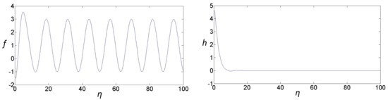
Figure 1. The figures above present graphical representations of (40) and (41) when $b=1,\overline{\phi }=1,A=1,B=1$.

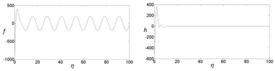
Figure 2. The figures above present graphical representations of (40) and (41) when $b=1,\overline{\phi }={\displaystyle \frac{\pi }{2}},A=10,B=10$.

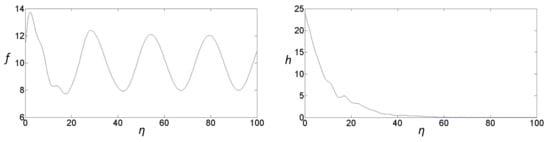
Figure 3. The figures above present graphical representations of (40) and (41) when $b=10,\overline{\phi }={\displaystyle \frac{\pi }{2}},A=1,B=1$.

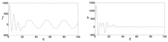
Figure 4. The figures above present graphical representations of (40) and (41) when $b=10,\overline{\phi }={\displaystyle \frac{\pi }{2}},A=10,B=10$.

From the figures above, the common physical laws in each graph are analyzed, and the physical laws of angular velocity and radial velocity with varying displacement can be inferred. In each graph, $f\left(\eta \right)$, which can reflect the angular velocity, approaches an oscillatory decreasing function while $\eta$ approaches infinity. Therefore, it can be concluded that angular velocity has upper and lower boundaries. Furthermore, $h\left(\eta \right)$, which can reflect the axial velocity, decays to zero when $\eta$ approaches infinity. Thus, the axial velocity is greatly affected by displacement and rapidly decreases within small displacement changes. Furthermore, according to the attenuation trend of f and h, it can be inferred that the thickness of the boundary layer becomes thinner with the flow direction, and the energy loss also decreases accordingly.

5. Conclusions

In this work, the homotopy renormalization (HTR) method has been employed to solve a specific form of reduced Navier–Stokes equations, known as Rasmussen’s problem. We successfully obtained global asymptotic solutions in closed form. The findings indicate that the HTR method offers a simple yet effective framework for deriving global approximations, as it completely avoids the handling of secular terms. Moreover, the obtained asymptotic solutions have a finite number of terms, providing significantly higher applicability than traditional series solutions or numerical solutions. Furthermore, this approach shows strong potential for addressing a wide range of nonlinear differential equations commonly encountered in mathematical physics. Some beneficial conclusions have been drawn, such as the inference that the thickness of the boundary layer becomes thinner with the flow direction, which has positive significance for the study of boundary layer physical phenomena.

References

- Buckingham, E. Construction for Direct-Reading Scales for the Slide Wire Bridge. Phys. Rev. 1903, 17, 382–383. [Google Scholar]
- Gell-Mann, M.; Low, F.E. Quantum electrodynamics at small distances. Phys. Rev. 1954, 95, 1300–1312. [Google Scholar]
- Goldenfeld, N.; Martin, O.; Oono, Y.; Liu, F. Anomalous dimensions and the renormalization group in a nonlinear diffusion process. Phys. Rev. Lett. 1990, 64, 1361–1364. [Google Scholar] [CrossRef]
- Chen, L.Y.; Goldenfeld, N.; Oono, Y. Renormalization-group theory for the modified porous-medium equation. Phys. Rev. A 1991, 44, 6544–6550. [Google Scholar] [CrossRef]
- Chen, L.Y.; Goldenfeld, N. Renormalization-group theory for the propagation of a turbulent burst. Phys. Rev. A 1992, 45, 5572–5577. [Google Scholar] [CrossRef] [PubMed]
- Goldenfeld, N.; Martin, O.; Oono, Y. Intermediate asymptotics and renormalization group theory. J. Sci. Comput. 1989, 4, 355–372. [Google Scholar] [CrossRef]
- Chen, L.Y.; Goldenfeld, N.; Oono, Y. Renormalization group and singular perturbations: Multiple scales, boundary layers, and reductive perturbation theory. Phys. Rev. E 1996, 54, 376. [Google Scholar] [CrossRef]
- Goldenfeld, N.; Martin, O.; Oono, Y. Asymptotics of partial differential equations and the renormalisation group. In Asymptotics Beyond All Orders; Springer: Boston, MA, USA, 1991; pp. 375–383. [Google Scholar]
- Kunihiro, T. A geometrical formulation of the renormalization group method for global analysis. Prog. Theor. Phys. 1995, 94, 503–514. [Google Scholar] [CrossRef]
- Kunihiro, T. A geometrical formulation of the renormalization group method for global analysis II: Partial differential equations. Jpn. J. Ind. Appl. Math. 1997, 14, 51–69. [Google Scholar] [CrossRef]
- Kunihiro, T. The renormalization-group method applied to asymptotic analysis of vector fields. Prog. Theor. Phys. 1997, 97, 179–200. [Google Scholar] [CrossRef]
- Kai, Y. Global solutions to two nonlinear perturbed equations by renormalization group method. Phys. Scr. 2016, 91, 025202. [Google Scholar] [CrossRef]
- Tu, T.; Cheng, G.; Liu, J.W. Improvement of Renormalization Group for Barenblatt Equation. Commun. Theor. Phys. 2004, 42, 290–294. [Google Scholar] [CrossRef]
- Tu, T.; Cheng, G.; Liu, J.W. Anomalous Dimension in the Solution of the Modified Porous Medium Equation. Commun. Theor. Phys. 2002, 37, 741–744. [Google Scholar] [CrossRef]
- Tu, T.; Cheng, G.; Liu, J.W. Anomalous Dimension in the Solution of a Nonlinear Diffusion Equation. J. Phys. A 2001, 34, 617–619. [Google Scholar] [CrossRef]
- Liu, C.S. The renormalization method based on the Taylor expansion and applications for asymptotic analysis. Nonlinear Dyn. 2017, 88, 1099–1124. [Google Scholar] [CrossRef]
- Kai, Y. Exact solutions and asymptotic solutions of one-dimensional domain walls in nonlinearly coupled system. Nonlinear Dyn. 2018, 92, 1665–1677. [Google Scholar] [CrossRef]
- Kai, Y.; Zheng, B.; Zhang, K.; Xu, W.; Yang, N. Exact and asymptotic solutions to magnetohydrodynamic flow over a nonlinear stretching sheet with a power-law velocity by the homotopy renormalization method. Phys. Fluids 2019, 31, 063606. [Google Scholar] [CrossRef]
- Liu, C. The renormalization method from continuous to discrete dynamical systems: Asymptotic solutions, reductions and invariant manifolds. Nonlinear Dyn. 2018, 94, 873–888. [Google Scholar] [CrossRef]
- Guan, J.; Kai, Y. Asymptotic Analysis to Two Nonlinear Equations in Fluid Mechanics by Homotopy Renormalisation Method. Z. Naturforschung A 2016, 71, 863–868. [Google Scholar] [CrossRef]
- Wang, C.; Gao, W. Asymptotic Analysis of Reduced Navier—Stokes Equations by Homotopy Renormalization Method. Rep. Math. Phys. 2017, 80, 29–37. [Google Scholar] [CrossRef]
- Xin, H. Asymptotic Analysis of a Nonlinear Problem on Domain Boundaries in Convection Patterns by Homotopy Renormalization Method. Z. Naturforschung A 2017, 72, 909–913. [Google Scholar] [CrossRef]
- Rasmussen, H. High Reynolds number flow between two inflnite rotating disks. J. Aust. Math. Soc. 1971, 12, 483–501. [Google Scholar] [CrossRef]
- Von Kármá, T. Uber läminare und terbulence Reibung. Zamm-J. Appl. Math. Mech. 1921, 1, 233–252. [Google Scholar]
- Kai, Y.; Zheng, B. Asymptotic analysis to free-convective boundary-layer problem by homotopy renormalization method. Mod. Phys. Lett. B 2019, 33, 1950083. [Google Scholar] [CrossRef]
- Kai, Y.; Zhang, K.; Yin, Z. HTR approach to the asymptotic solutions of supersonic boundary layer problem: The case of slow acoustic waves interacting with streamwise isolated wall roughness. Math. Sci. 2021, 17, 21–30. [Google Scholar] [CrossRef]
Disclaimer/Publisher’s Note: The statements, opinions and data contained in all publications are solely those of the individual author(s) and contributor(s) and not of MDPI and/or the editor(s). MDPI and/or the editor(s) disclaim responsibility for any injury to people or property resulting from any ideas, methods, instructions or products referred to in the content. |
© 2025 by the authors. Licensee MDPI, Basel, Switzerland. This article is an open access article distributed under the terms and conditions of the Creative Commons Attribution (CC BY) license (https://creativecommons.org/licenses/by/4.0/).