Article

Parameter Estimation of General Uncertain Differential Equations via the Principle of Least Squares with Its Application in Economic Field

School of Economics, Shanghai University, Shanghai 200444, China
*
Author to whom correspondence should be addressed.
Symmetry 2025, 17(10), 1594; https://doi.org/10.3390/sym17101594
Submission received: 15 August 2025 / Revised: 13 September 2025 / Accepted: 17 September 2025 / Published: 24 September 2025

Abstract

The parameter estimation problem is one of the research hotspots in the field of uncertain differential equations. However, most studies at present focus on parameter estimation based on residuals of uncertain differential equations, which relies strictly on the solvability of residuals. In view of this disadvantage, this paper derives a symmetrical statistical invariant, which is different from residuals based on the difference scheme, and proposes the least squares estimation of general uncertain differential equations based on the statistical invariant and the principle of least squares. In order to consider parameter estimation in more general cases, this paper also studies the least squares estimation of time-varying parameters in general uncertain differential equations and designs corresponding to numerical algorithms to calculate the numerical solutions of these least squares estimations. Finally, this paper also proposes two numerical examples and an empirical study to illustrate the above methods.

1. Introduction

In order to more realistically describe time-varying systems in the real world, there are two mathematical tools in total. One is the stochastic differential equation based on probability theory (proposed by Kolmogorov [1]), and the other is the uncertain differential equation based on uncertainty theory (proposed by Liu [2]). Since their proposal, stochastic differential equations have been extensively studied by numerous scholars, giving rise to numerous research branches, and successfully applied in fields such as financial research, social sciences, physical systems, and chemical evolution.
Although stochastic differential equations have produced many achievements, most studies on stochastic differential equations only focus on their theoretical results and do not discuss their applicability based on actual data. In other words, the theoretical basis of stochastic differential equations is probability theory, and the premise that probability theory can reasonably model the real world is based on the condition that the frequency of the observed data we obtain is stable enough, which is a strong enough condition. In fact, a large number of empirical studies have proven that the observed data in practice do not meet the conditions of frequency stability. At this time, the distribution function generated based on historical data cannot be close enough to the actual frequency of the research object. If it is regarded as a probability distribution function, and the stochastic differential equation based on probability theory is used to describe the research object, unreasonable results will be obtained. For example, Yang and Ke [3] showed that stochastic differential equations are not suitable for portraying Shanghai interbank offered rates, which in turn shows that the actual data in the financial system cannot meet the frequency stability conditions. Yang and Liu [4] illustrated that if population size data are characterized by using stochastic partial differential equations, unstable frequency results will also be obtained, and Liu et al. [5] modeled online ride-hailing data in Beijing, China, by using the stochastic renewal process, and obtained results that violate common sense. These results all show that the actual data in the social system are also frequency unstable. In addition to showing, from the perspective of empirical research, that stochastic differential equations are not suitable for modeling the real world, Liu [6] also pointed out that the velocity of Brownian motion B t is infinite (that is, the derivative of Brownian motion B t at any moment is a normal random variable whose expected value is 0, and the variance is infinite) and theoretically deduced the paradox of the stochastic differential equation. Since the real world cannot guarantee the fulfillment of the assumption of frequency stability, stochastic differential equations cannot reasonably model time-varying systems in the real world. In order to solve the problem of how to reasonably describe the phenomenon of frequency instability, Liu [2] proposed uncertainty theory in 2007, which is an axiomatic mathematical system based on normativity, duality, subadditivity, and the product axioms. To date, uncertainty theory has been studied by many scholars and has spawned many research branches, such as the uncertain differential equation [7], uncertain optimal control [8], uncertain renewal process [9], uncertain graph [10], etc.
Among the many theoretical branches of uncertainty theory, uncertain differential equations hold a crucial position as a powerful tool for characterizing the evolution of dynamic systems over time under uncertain environments. They were proposed by Liu [11] as a class of differential equations driven by Liu processes. Since their proposal, they has attracted the attention of many scholars. In theoretical research, Chen and Liu [12] first investigated the existence and uniqueness conditions for solutions of uncertain differential equations. Based on this work, Liu [13] began research on stability for uncertain differential equations. Subsequently, Yao et al. [14] proposed several stability theorems, further advancing the field of stability analysis for uncertain differential equations. The Yao–Chen formula developed by Yao and Chen [15] is a significant contribution to the study of uncertain differential equations, which links uncertain differential equations with ordinary differential equations, demonstrating that the solution to an uncertain differential equation can be represented by the solutions of a family of ordinary differential equations. Therefore, the Yao–Chen formula provides an accurate and elegant way to obtain numerical solutions to uncertain differential equations. Based on this, Yao and Chen [15] first proposed a numerical method for solving uncertain differential equations. Based on the above pioneering work, many scholars have devoted themselves to researching and improvementing on the theoretical work of uncertain differential equations, producing a large number of results.
The application of uncertain differential equations in practice is the problem of parameter estimation, which is also the current research hotspot. However, the current research on parameter estimation of uncertain differential equations mainly focuses on methods based on the residuals of uncertain differential equations. Although the parameter estimation methods based on the residuals have high accuracy, such methods strictly rely on the existence of analytical solutions to uncertain differential equations or the existence of the inverse uncertainty distributions of their solutions. As we all know, only a few uncertain differential equations can obtain corresponding analytical solutions, and only regular uncertain differential equations can be solved numerically and obtain inverse uncertainty distributions. Therefore, parameter estimation methods based on the residuals of uncertain differential equations have certain limitations. In order to study the least squares estimation of general uncertain differential equations, this paper will construct a symmetric statistical invariant based on the difference scheme of uncertain differential equations, and study its least squares estimation based on this statistical invariant and the principle of least squares. Specifically, the main contributions of this paper are as follows:
  • A statistical invariant based on the difference scheme of uncertain differential equations has been constructed, and for general uncertain differential equations, the analytical expression of this statistical invariant can be obtained. This resolves the problem that the residual-based parameter estimation method for uncertain differential equations is limited by the solvability of the uncertainty distribution or the inverse uncertainty distribution of the solution.
  • The least squares estimations of the constant parameters and time-varying parameters of general uncertain differential equations are proposed. This solves the problem of applying the least squares method based on uncertainty distribution to the parameter estimation of constant parameters and time-varying parameters in uncertain differential equations.
  • Two numerical algorithms are designed to solve the numerical solution of the aforementioned least squares estimations.
  • Two numerical examples and an empirical study are provided to illustrate the corresponding methods proposed in this paper.

2. Literature Review of Parameter Estimation of Uncertain Differential Equations

Parameter estimation of uncertain differential equations is the current research hotspot in this field and is also the research topic of this paper. Therefore, this section will conduct a literature review on parameter estimation of uncertain differential equations.
Parameter estimation for uncertain differential equations originated from the work of Yao and Liu [16], which first proposed moment estimation for uncertain differential equations based on their difference scheme and the method of moments. However, when there are too many unknown parameters, moment estimation may not be possible. To address this issue, Liu [17] further developed the generalized moment estimation of uncertain differential equations by minimizing the sum of squares of the deviations between each order of sample moments and each order of population moments. Furthermore, Sheng et al. [18] investigated a least squares estimation for uncertain differential equations by minimizing the noise terms. Yang et al. [19] explored the minimum covering estimation by ensuring that the observed data fall within a reasonable range of the α paths. Liu and Liu [20] borrowed the idea of uncertain maximum likelihood to present the maximum likelihood estimation for uncertain differential equations. These works are early achievements in this field and are all based on difference schemes for uncertain differential equations. Their disadvantage is that these difference schemes can introduce errors, and this error is particularly significant when the time step of the observation data is not sufficiently small, which is usually impossible to control.
In order to address the problems caused by the difference schemes, Liu and Liu [21] proposed the concept of residuals for uncertain differential equations and established a precise connection between uncertain differential equations and observed data. Since then, the focus of many scholars has shifted to residual-based parameter estimation methods for uncertain differential equations. Based on the residuals of uncertain differential equations, Liu and Liu [21] first studied residual-based moment estimation. Then, Liu and Liu borrowed the ideas of uncertain maximum likelihood and least squares criteria to explore residual-based maximum likelihood estimation (Liu and Liu [22]) and residual-based least squares estimation (Liu and Liu [23]), respectively. In addition, scholars have also explored the parameter estimation of multi-factor uncertain differential equations, including residual-based moment estimation (Yao and Sheng [24]), residual-based maximum likelihood estimation (Liu et al. [25]), and residual-based least squares estimation (Wu and Liu [26]). Some scholars have also conducted research on parameter estimation of a class of uncertain partial differential equations. For example, Yang and Liu [4] studied residual-based moment estimation of a class of uncertain partial differential equations, and Yang and Liu [27] proposed residual-based least squares estimation and applied it to modeling the Chinese population. These studies are precisely the focus of parameter estimation in uncertain differential equations at the methodological level, and the advantage of these methods is that they are based on residuals that accurately connect the uncertain differential equations to the observed data, resulting in relatively more accurate results. However, their disadvantage is that they rely heavily on the solvability of the residuals. For the general uncertain differential equations that do not satisfy regularity conditions, the residuals are essentially unobtainable. In such cases, these methods will fail, and we will be forced to resort to parameter estimation methods based on difference schemes.

3. Preliminary

In this section, we will provide some concepts and theorems about uncertainty theory and uncertain differential equations to ensure that readers can understand the following content more easily.
The uncertain measure is the foundation of uncertainty theory, which is actually a set function defined on a σ -algebra, and the specific definition is as follows:
Definition 1
(Liu [2]). Let Γ denote the universal set, and let Ł denote the σ-algebra over Γ. If the measurable set function M defined on the σ-algebra Ł Ł satisfies the following three conditions, then the measurable set function M is called an uncertain measure, and thus ( Γ , Ł , M ) is called an uncertainty space:
  • Normality Axiom: M { Γ } = 1 for the universal set Γ.
  • Duality Axiom: For any event Λ Ł , M { Λ } + M { Λ c } = 1 always holds.
  • Subadditivity Axiom: For every countable sequence of events Λ 1 , Λ 2 , ,
    M i = 1 Λ i i = 1 M { Λ i }
    always holds.
For the purpose of obtaining the uncertain measure of a composite event, the product uncertain measure M on the product σ -algebra Ł was defined by Liu [13] by assuming it follows the product axiom. That is, let ( Γ i , Ł i , M i ) , i = 1 , 2 , be a sequence of uncertainty spaces. If the uncertain measure M defined on the σ -algebra Ł satisfies
M i = 1 Λ i = i = 1 M i { Λ i } ,
where Λ i Ł for i = 1 , 2 , , then the uncertain measure M is called a product uncertain measure. Based on the uncertainty space ( Γ , Ł , M ) , an instrument used to describe quantities in uncertain environments is the uncertain variable, which was defined by Liu [2] as a measurable function from an uncertainty space ( Γ , Ł , M ) to the set of real numbers and was denoted by ξ , i.e., the set
{ ξ B } = { γ Γ ξ ( γ ) B }
is always an event for any Borel set B of real numbers. Subsequently, in order to facilitate the calculation of uncertain variables in practical situations, the uncertainty distribution of an uncertain variable ξ was also defined by Liu [2] as
Φ ( x ) = M { ξ x } , x .
Example 1.
If the uncertain variable ξ has a normal uncertainty distribution
Φ ( x ) = 1 + exp π ( e x ) 3 σ 1 , x ,
then it is called a normal uncertain variable, and is represented as N ( e , σ ) , where e is the expected value and σ is the standard deviation. In addition, a normal uncertainty distribution is called standard if e = 0 and σ = 1 .
In practice, only independent uncertain variables can be subjected to operations. In order to define what kind of uncertain variables are independent, Liu [13] suggested that if the uncertain variables ξ 1 , ξ 2 , , ξ n satisfy
M i = 1 n ( ξ i B i ) = i = 1 n M ξ i B i
for any Borel sets B 1 , B 2 , , B n of real numbers, then the uncertain variables ξ 1 , ξ 2 , , ξ n can be called independent. Furthermore, in order to provide a more accurate description of time-varying systems in uncertain environments, the Liu process C t was defined by Liu [13] as follows:
Definition 2.
An uncertain process C t is said to be a Liu process if
  • (i) C 0 = 0 , and almost all sample paths are Lipschitz continuous;
  • (ii) C t has stationary and independent increments;
  • (iii) every increment C s + t C s is a normal uncertain variable with expected value 0 and standard deviation t.

4. Symmetric Statistical Invariant Based on Difference Scheme

In this section, we consider the general uncertain differential equation expressed in the following form:
d X t = f ( t , X t ; θ ) d t + g ( t , X t ; θ ) d C t ,
where f ( t , x ) and g ( t , x ) are two continuous real-valued functions satisfying the existence and uniqueness conditions for the solution of uncertain differential Equation (1), i.e., linear growth condition
| f ( t , x ) | + | g ( t , x ) | L 1 + | x | , t 0 , x , y R ,
and Lipschitz condition
| f ( t , x 1 )     f ( t , x 2 ) |   +   | g ( t , x 1 )     g ( t , x 2 ) |     L | x 1 x 2 | , t     0 , x 1 , x 2 R
for some constant L, θ is a vector of unknown parameters to be estimated, and C t is a Liu process.
Suppose also that there exists a set of observed data
x t 1 , x t 2 , , x t n
of the solution X t to uncertain differential Equation (1) at time points t 1 , t 2 , , t n with t 1 < t 2 < < t n , respectively. In order to link the uncertain differential Equation (1) with the observed data (2), we first discretize uncertain differential Equation (1) at the observed time points t 1 , t 2 , , t n . That is, we choose to write uncertain differential Equation (1) into the Euler difference form,
X t i = X t i 1 + f ( t i 1 , X t i 1 ; θ ) ( t i t i 1 ) + g ( t i 1 , X t i 1 ; θ ) ( C t i C t i 1 ) , i = 2 , 3 , , n .
Based on the above Euler difference form, we can obtain
X t i X t i 1 f ( t i 1 , X t i 1 ; θ ) ( t i t i 1 ) g ( t i 1 , X t i 1 ; θ ) ( t i t i 1 ) = C t i C t i 1 t i t i 1
for i = 2 , 3 , , n . For each index i with 2 i n , it follows from Definition 2 that the increments C t i C t i 1 of the Liu process C t over the time intervals [ t i 1 , t i ] are a normal uncertain variable with expected value 0 and standard deviation t i t i 1 . That is,
C t i C t i 1 N ( 0 , t i t i 1 ) .
Thus, we have
C t i C t i 1 t i t i 1 1 t i t i 1 × N ( 0 , t i t i 1 ) = N ( 0 , 1 ) .
Therefore, it is easy to infer that C t i C t i 1 t i t i 1 , i = 2 , 3 , , n are always independent of each other and
C t i C t i 1 t i t i 1 N ( 0 , 1 ) , i = 2 , 3 , , n
always holds. By using the above transformation formula of the Euler difference form of uncertain differential Equation (1), we can also infer that
X t i X t i 1 f ( t i 1 , X t i 1 ; θ ) ( t i t i 1 ) g ( t i 1 , X t i 1 ; θ ) ( t i t i 1 ) , i = 2 , 3 ,
are always independent of each other and
X t i X t i 1 f ( t i 1 , X t i 1 ; θ ) ( t i t i 1 ) g ( t i 1 , X t i 1 ; θ ) ( t i t i 1 ) N ( 0 , 1 ) , i = 2 , 3 , , n
always holds. For the sake of convenience, we write
ξ i = X t i X t i 1 f ( t i 1 , X t i 1 ; θ ) ( t i t i 1 ) g ( t i 1 , X t i 1 ; θ ) ( t i t i 1 ) , i = 2 , 3 , , n .
Then, it follows from the above analysis that
ξ i N ( 0 , 1 ) , i = 2 , 3 , , n .
On the other hand, we substitute the observed data (2) into
X t i X t i 1 f ( t i 1 , X t i 1 ; θ ) ( t i t i 1 ) g ( t i 1 , X t i 1 ; θ ) ( t i t i 1 ) , i = 2 , 3 , , n ,
and write
h i ( θ ) = x t i x t i 1 f ( t i 1 , x t i 1 ; θ ) ( t i t i 1 ) g ( t i 1 , x t i 1 ; θ ) ( t i t i 1 ) , i = 2 , 3 , , n .
Note that h i ( θ ) , i = 2 , 3 , , n are n 1 real-valued functions with respect to the vector of unknown parameters θ and can be regarded as the samples of ξ i , i = 2 , 3 , , n , respectively. That is, we should have
h 2 ( θ ) , h 3 ( θ ) , , h n ( θ ) N ( 0 , 1 ) .
At this point, we have constructed a series of real-valued functions h i ( θ ) , i = 2 , 3 , , n of the vector of unknown parameters θ based on uncertain differential Equation (1) and its observed data (2), and processed the population distribution of the real-valued functions h i ( θ ) , i = 2 , 3 , , n as a statistical invariant N ( 0 , 1 ) . Since the uncertainty distribution of N ( 0 , 1 ) is symmetric about the origin, this statistical invariant is also called symmetric.

5. Least Squares Estimation of General Uncertain Differential Equations

In order to apply the least squares principle when estimating unknown parameters, Liu and Liu [23] proposed a least squares estimation based on uncertainty distribution by minimizing the sum of squares of the deviations between the empirical distribution of samples and the distribution function of the population. In this section, we will apply this method to the parameter estimation of general uncertain differential equations.

5.1. Least Squares Estimation Based on Uncertainty Distribution

Assume that there exists a population ξ in uncertain environments, whose uncertainty distribution is denoted by Φ θ ( x ) , and θ is a vector of unknown parameters. Suppose also there exists a set of observed data
x 1 , x 2 , , x n
which can be regarded as the observed values of the population ξ . Based on this, Liu and Liu [23] suggested that the least squares estimation of the vector of unknown parameters θ should minimize the deviations between the empirical distribution of observed data x 1 , x 2 , , x n and the uncertainty distribution Φ θ ( x ) . That is, the least squares estimation θ ^ should be the solution of
min θ i = 1 n Φ θ ( x i ) F ( x i ) 2 .
Here, F ( x ) is the empirical distribution of observed data x 1 , x 2 , , x n and is defined as
F ( x ) = 1 n i = 1 n I ( x i x ) ,
where
I ( x i x ) = 1 if x i x 0 otherwise
is the indicator function.

5.2. Least Squares Estimation of General Uncertain Differential Equations with Constant Parameters

For the general uncertain differential Equation (1) with the vector of unknown parameters θ and the given observed data (2), we can always obtain a set of independent and identically distributed samples of the symmetric statistical invariant N ( 0 , 1 ) , i.e.,
h 2 ( θ ) , h 3 ( θ ) , , h n ( θ ) N ( 0 , 1 ) .
Next, we will apply the least squares estimation method based on the uncertainty distribution to estimate the unknown parameter vector θ . It is easy to infer that the empirical distribution of h 2 ( θ ) , h 3 ( θ ) , , h n ( θ ) is
F ( x | θ ) = 1 n 1 j = 2 n I ( h j ( θ ) x ) ,
and the uncertainty distribution of N ( 0 , 1 ) is
Φ ( x ) = 1 1 + exp π x 3 .
Then, it follows from (7) that the least squares estimation of unknown parameter vector θ can be obtained by solving the following minimization problem:
min θ i = 2 n 1 1 + exp π h i ( θ ) 3 1 n 1 j = 2 n I ( h j ( θ ) h i ( θ ) ) 2 .
The solution θ ^ of the above minimization problem is also called the least squares estimation of the general uncertain differential Equation (1).
In order to ensure that the solution to the least squares estimation can be truly achieved, we will design a numerical algorithm.
  • Numerical algorithms for least squares estimation
Step 0: Input the general uncertain differential equation
d X t = f ( t , X t ; θ ) d t + g ( t , X t ; θ ) d C t
that needs to be estimated and the observed data x t 1 , x t 2 , , x t n .
Step 1: Determine the feasible regions Θ of the unknown parameters vector θ .
Step 2: For each θ Θ , compute h j ( θ ) by
h j ( θ ) = x t j x t j 1 f ( t j 1 , x t j 1 ; θ ) ( t j t j 1 ) g ( t j 1 , x t j 1 ; θ ) ( t j t j 1 )
for j = 2 , 3 , , n .
Step 3: Set i = 2 and O b j θ = 0 .
Step 4: Set
O b j θ = O b j θ + 1 1 + exp π h i ( θ ) 3 1 n 1 j = 2 n I ( h j ( θ ) h i ( θ ) ) 2 ,
and i = i + 1 .
Step 5: If i n , then go to Step 4.
Step 6: Find θ ^ such that O b j θ reaches its minimum value by using MATLAB with version number of ‘9.13.0.2049777 (R2022b)’.
Step 7: Output θ ^ .

6. Least Squares Estimation of General Uncertain Differential Equations with Time-Varying Parameters

Generally speaking, the unknown parameters in uncertain differential equations tend to be time-varying rather than constant. Building on this, we will further investigate the least squares estimation problem for uncertain differential equations with time-varying parameters.
Here, we consider the following uncertain differential equations with time-varying parameters,
d X t = f ( t , X t ; θ t ) d t + g ( t , X t ; θ t ) d C t ,
where all the assumptions are the same as those in (1), with the exception that θ t is assumed to be a time-varying parameter related to time t. On the other hand, we also assume that there exists a set of observed data
x t 1 , x t 2 , , x t n
of the solution X t to uncertain differential Equation (11) at time points t 1 , t 2 , , t n with t 1 < t 2 < < t n , respectively. By using the method proposed in Section 4, we can also obtain n 1 samples of the symmetric statistical invariant N ( 0 , 1 ) , where the time-varying parameter θ t serves as the independent variable. That is,
h 2 ( θ t ) , h 3 ( θ t ) , , h n ( θ t ) N ( 0 , 1 ) .
Before estimating the time-varying parameters θ t , we first set a sliding window k, which is a given positive integer within an appropriate range. Then, for each index j with 2 j n k + 1 , the sequence h j ( θ t ) , h j + 1 ( θ t ) , , h j + k 1 ( θ t ) can also be regarded as a set of samples of N ( 0 , 1 ) . In this time, since the time period for the observed data is solely within the interval [ t j 1 , t j + k 1 ] , we can assume that the variations of the time-varying parameters θ t within this period are small. Thus, the time-varying parameters θ t can be regarded as a constant θ t j 1 in this period. Therefore, we can obtain the least squares estimation θ ^ t j 1 of θ t j 1 by solving the following minimization problem:
min θ t j 1 i = j j + k 1 1 1 + exp π h i ( θ t j 1 ) 3 1 k l = j j + k 1 I ( h l ( θ t j 1 ) h i ( θ t j 1 ) ) 2 .
Iterating over j from 2 to n k + 1 , and repeating the above operation, we can obtain a set of least squares estimations
θ ^ t 1 , θ ^ t 2 , , θ ^ t n k
for the time-varying parameters θ t . Then, we select an appropriate uncertain regression model to fit the set of least squares estimations (15), and the resulting regression equation is just the least squares estimation of the time-varying parameters θ t .
In order to ensure that the solution to the least squares estimation of the time-varying parameters θ t can be truly achieved, we will design a numerical algorithm.
  • Numerical algorithms for least squares estimation with time-varying parameters
Step 0: Input the general uncertain differential equation with time-varying parameters,
d X t = f ( t , X t ; θ t ) d t + g ( t , X t ; θ t ) d C t ,
that needs to be estimated, the observed data x t 1 , x t 2 , , x t n , and the sliding window k.
Step 1: Determine the feasible regions Θ t of the unknown parameters vector θ t .
Step 2: Set j = 2 .
Step 3: For each θ t j 1 Θ t j 1 , compute h i ( θ t j 1 ) by
h i ( θ t j 1 ) = x t i x t i 1 f ( t i 1 , x t i 1 ; θ t j 1 ) ( t i t i 1 ) g ( t i 1 , x t i 1 ; θ t j 1 ) ( t i t i 1 )
for i = j , j + 1 , , j + k 1 .
Step 4: Set i = j and O b j θ t j 1 = 0 .
Step 5: Set
O b j θ t j 1 = O b j θ t j 1 + 1 1 + exp π h i ( θ t j 1 ) 3 1 k l = j j + k 1 I ( h l ( θ t j 1 ) h i ( θ t j 1 ) ) 2 ,
and i = i + 1 .
Step 6: If i j + k 1 , then go to Step 5.
Step 7: Find θ ^ t j 1 such that O b j θ t j 1 reaches its minimum value by using MATLAB, and set j = j + 1 .
Step 8: If j n k + 1 , then go to Step 3.
Step 9: Select the uncertain regression model to fit θ ^ t 1 , θ ^ t 2 , , θ ^ t n k , and obtain the regression equation θ ^ t .
Step 10: Output θ ^ t .

7. Numerical Examples

In this section, two numerical examples will be provided to illustrate the least squares estimation of the constant parameters and time-varying parameters that were previously proposed.
Example 2.
Consider the following linear uncertain differential equation:
d X t = a d t + b d C t ,
where a and b are two parameters that need to be estimated. Suppose also there is a dataset consisting of 45 sets of observational data ( t i , x t i ) , i = 1 , 2 , , 45 , as shown in Table 1.
In order to use linear uncertain differential Equation (16) to describe the observational data in Table 1, we first need to estimate the unknown parameters a and b. By substituting the observational data ( t i , x t i ) , i = 1 , 2 , , 45 into (4), we can obtain
h i ( a , b ) = x t i x t i 1 a ( t i t i 1 ) b ( t i t i 1 ) = 1 b x t i x t i 1 t i t i 1 a , i = 2 , 3 , , 45 .
Then, it follows from (10) that the least squares estimation of ( a , b ) solves
min a , b i = 2 45 1 1 + exp π 3 b x t i x t i 1 t i t i 1 a 1 44 j = 2 45 I x t j x t j 1 t j t j 1 x t i x t i 1 t i t i 1 2 .
By using MATLAB to solve the above minimization problem, the optimal solution can be obtained as
a ^ = 0.9406 , b ^ = 0.5105 .
Thus, the estimated linear uncertain differential equation is
d X t = 0.9406 d t + 0.5105 d C t .
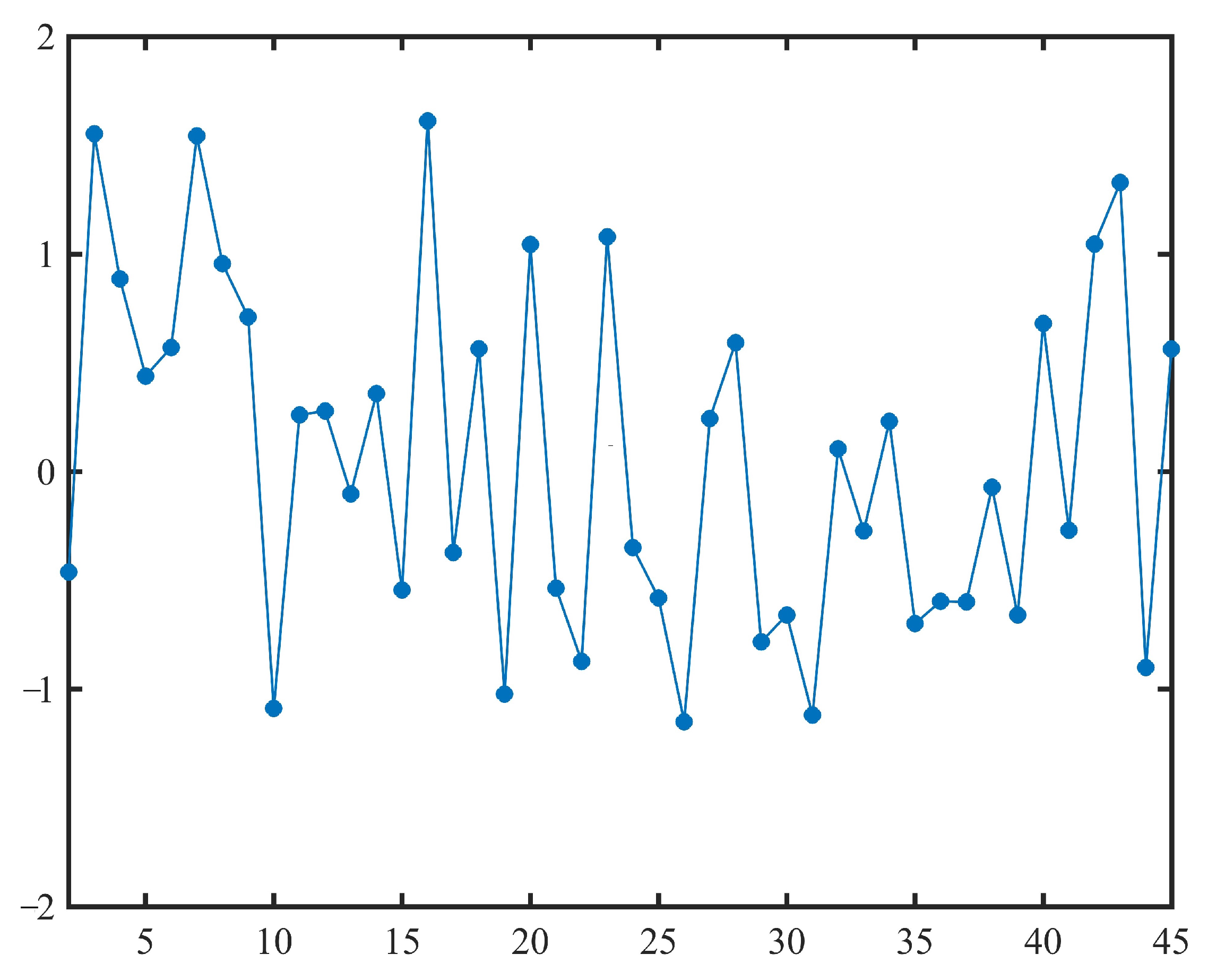
By substituting the estimated a ^ and b ^ into (17), we can obtain 44 samples h 2 , h 3 , , h 45 of the normal uncertainty distribution N ( 0 , 1 ) , as shown in Table 2 and Figure 1.
If the estimated parameters a ^ and b ^ are appropriate, then the obtained h 2 , h 3 , , h 45 should indeed be a set of samples of normal uncertainty distribution N ( 0 , 1 ) . That is, the test of the estimated parameters a ^ and b ^ is equivalent to testing whether h 2 , h 3 , , h 45 is a set of samples of N ( 0 , 1 ) , whose null hypothesis is
e = 0   a n d   σ = 1
and the alternative hypothesis is
e 0   o r   σ 1 ,
where e is the expected value, and σ is the standard deviation of the normal population distribution of h 2 , h 3 , , h 45 , respectively. The uncertain hypothesis test presented by Ye and Liu [28] tests whether the above hypothesis test problem for a given significance level α = 0.05 is
W = { ( h 2 , h 3 , , h 45 ) : t h e r e   a r e   a t   l e a s t   3   o f   i n d e x e s   i s   w i t h   2 i 45 s u c h   t h a t   h i < Φ 1 α 2   o r   h i > Φ 1 1 α 2 ,
where
Φ 1 α = 3 π ln α 1 α
is the inverse uncertainty distribution of N ( 0 , 1 ) . As shown in Table 2 and Figure 1, it is easy to see that all the points in h 2 , h 3 , , h 45 are within the interval
Φ 1 α 2 , Φ 1 1 α 2 = [ 2.0198 , 2.0198 ] .
Thus, we obtain
( h 2 , h 3 , , h 45 ) W .
That is, the obtained h 2 , h 3 , , h 45 is indeed a set of samples of normal uncertainty distribution N ( 0 , 1 ) . Therefore, the estimated parameters a ^ and b ^ are appropriate.
Example 3.
Consider the following exponential uncertain differential equation,
d X t = μ t X t d t + σ t X t d C t ,
where μ t and σ t are two time-varying parameters that need to be estimated. Suppose also there is a dataset consisting of 120 sets of observational data ( t i , x t i ) , i = 1 , 2 , , 120 , as shown in Table 3. In order to use exponential uncertain differential Equation (19) to describe the observational data in Table 3, we first need to estimate the time-varying unknown parameters μ t and σ t .
Take k = 20 as the sliding window for estimating μ t and σ t . Then, for each index j with 2 j 101 , we choose ( t i , x t i ) , i = j 1 , j , , j + 19 as the observational data for estimating unknown parameters μ t j 1 and σ t j 1 . By substituting ( t i , x t i ) , i = j 1 , j , , j + 19 into (4), we can obtain
h i ( μ t j 1 , σ t j 1 ) = x t i x t i 1 μ t j 1 x t i 1 ( t i t i 1 ) σ t j 1 x t i 1 ( t i t i 1 ) = 1 σ t j 1 x t i x t i 1 x t i 1 ( t i t i 1 ) μ t j 1
with i = j 1 , j , , j + 19 . Then, it follows from (14) that the least squares estimation of ( μ t j 1 , σ t j 1 ) solves
min μ t j 1 , σ t j 1 i = j j + 19 1 + exp π 3 σ t j 1 x t i x t i 1 x t i 1 ( t i t i 1 ) μ t j 1 1 1 20 l = j j + 19 I x t l x t l 1 x t l 1 ( t l t l 1 ) x t i x t i 1 x t i 1 ( t i t i 1 ) ) 2 .
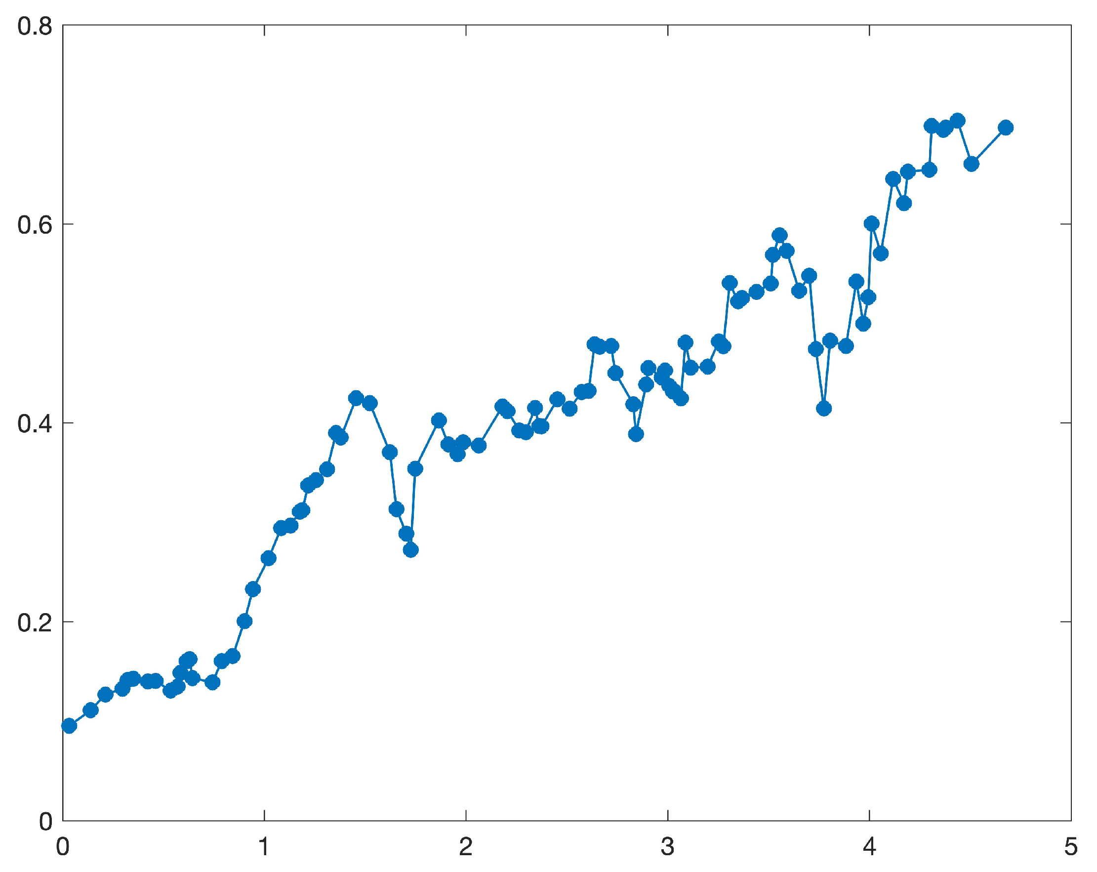
By using MATLAB to solve the above minimization problem, we can obtain the least squares estimation ( μ ^ t j 1 , σ ^ t j 1 ) . Iterating over j from 2 to 101, and repeating the above operation, we can obtain a set of least squares estimations ( μ ^ t j 1 , σ ^ t j 1 ) , j = 2 , 3 , , 101 , as shown in Table 4 and Figure 2 and Figure 3.
Next, we should choose appropriate regression models to fit the estimated μ ^ t j and σ ^ t j with j = 1 , 2 , , 100 . It is easy to see from Figure 2 and Figure 3 that we can choose the linear regression model to fit them. At first, we assume that the estimated μ ^ t j , j = 1 , 2 , , 100 can be fitted by
μ t = β 1 + β 2 t .
Then, β 1 and β 2 can be obtained by solving
min β 1 , β 2 j = 1 100 μ ^ t j β 1 β 2 t j 2 ,
which are
β 2 = j = 1 100 μ ^ t j 1 100 j = 1 100 μ ^ t j t j 1 100 j = 1 100 t j j = 1 100 t j 1 100 j = 1 100 t j 2 = 0.1337
and
β 1 = 1 100 j = 1 100 μ ^ t j β 2 1 100 j = 1 100 t j = 0.7484 .
That is, the time-varying parameter μ t can be fitted by
μ ^ t = 0.7484 0.1337 t .
Similarly, we can also assume that the estimated σ ^ t j , j = 1 , 2 , , 100 can be fitted by
σ t = β 3 + β 4 t ,
and β 3 and β 4 can be obtained as
β 3 = j = 1 100 σ ^ t j 1 100 j = 1 100 σ ^ t j t j 1 100 j = 1 100 t j j = 1 100 t j 1 100 j = 1 100 t j 2 = 0.1170
and
β 4 = 1 100 j = 1 100 σ ^ t j β 2 1 100 j = 1 100 t j = 0.1230 .
Thus, the time-varying parameter σ t can be fitted by
σ ^ t = 0.1230 + 0.1170 t ,
and the estimated exponential uncertain differential equation is
d X t = ( 0.7484 0.1337 t ) X t d t + ( 0.1230 + 0.1170 t ) X t d C t
immediately.
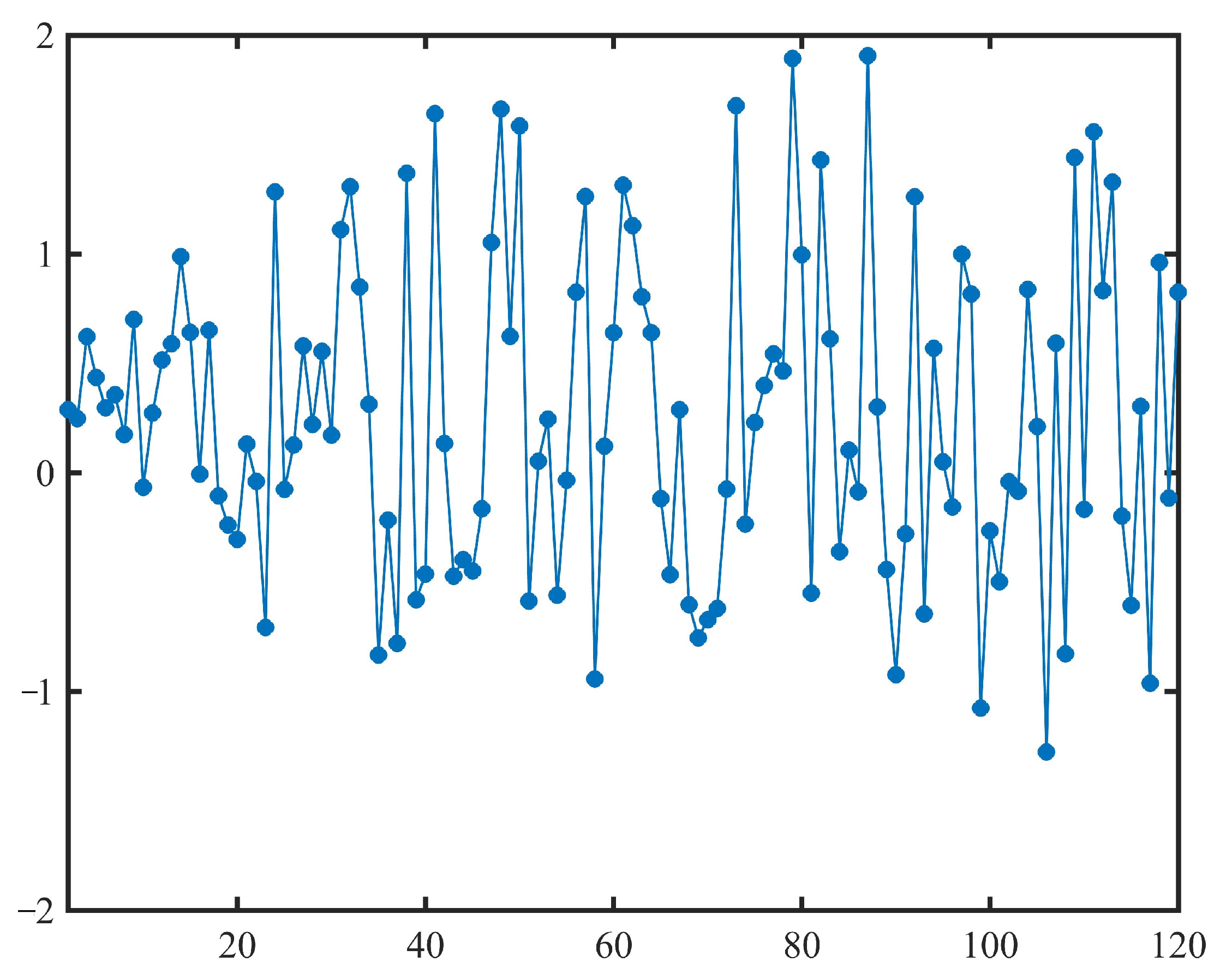
By substituting the estimated μ ^ t and σ ^ t into (20), we can obtain 119 samples h 2 , h 3 , , h 120 of the normal uncertainty distribution N ( 0 , 1 ) , as shown in Table 2 and Figure 1. In order to test whether the estimated time-varying parameters μ ^ t and σ ^ t are appropriate, it follows from the analysis of Example 2 that the test should be
W = { ( h 2 , h 3 , , h 120 ) : t h e r e   a r e   a t   l e a s t   6   o f   i n d e x e s   i s   w i t h   2 i 120 s u c h   t h a t   h i < Φ 1 α 2   o r   h i > Φ 1 1 α 2 ,
for a given significance level α = 0.05 , where
Φ 1 α = 3 π ln α 1 α
is the inverse uncertainty distribution of N ( 0 , 1 ) . As shown in Table 5 and Figure 4, it is easy to see that all the points in h 2 , h 3 , , h 120 are within the interval
Φ 1 α 2 , Φ 1 1 α 2 = [ 2.0198 , 2.0198 ] .
Thus, we obtain
( h 2 , h 3 , , h 120 ) W .
That is, the obtained time-varying parameters μ ^ t and σ ^ t are indeed a set of samples of normal uncertainty distribution N ( 0 , 1 ) . Therefore, the estimated time-varying parameters μ ^ t and σ ^ t are appropriate.

8. The Application in Economic Field

In this section, we will apply the method proposed in this paper to model stock prices and compare it with the method based on stochastic differential equations.

8.1. Data Source

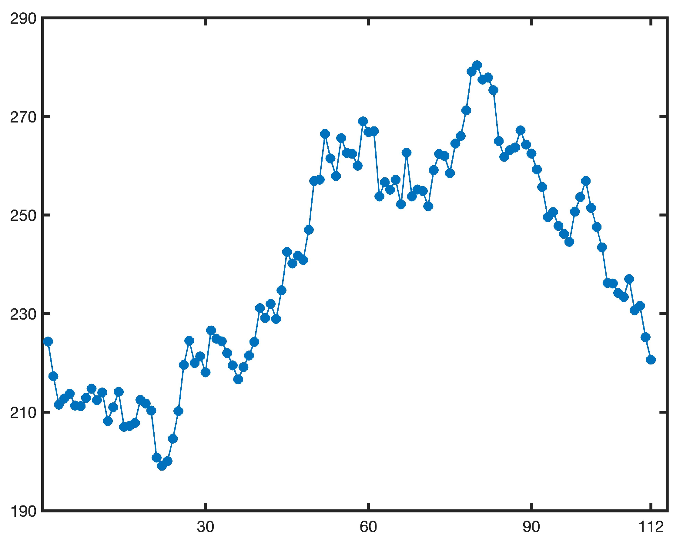
Anhui Gujinggong Liquor Co., Ltd. (Bozhou, China) is the core enterprise of Gujing Group and is the first liquor enterprise in China to issue both A shares and B shares. The stock prices of this company can to some extent reflect the fluctuations of the Chinese liquor market. In order to model the stock prices of Anhui Gujinggong Liquor Co., Ltd. (stock code: 000596.SZ), listed on the Shenzhen Stock Exchange, we collected the closing prices of the company’s stocks for all trading days from 1 January 2024 to 21 June 2024, with the currency unit being RMB. The data were sourced from the official historical trading records of Anhui Gujinggong Liquor Co., Ltd. provided by Sina Finance, which can be accessed via the webpage link (https://finance.sina.com.cn/realstock/company/sz000596/nc.shtml, accessed on 12 September 2025). The data were obtained on 12 September 2025, and a total of 112 valid data samples were obtained. The specific details of the closing prices can be seen in Table 6, while the trend of the closing prices can be seen in Figure 5.

8.2. Uncertain Stock Prices Model

Let i = 1 , 2 , , 112 denote the trading days from 1 January 2024 to 21 June 2024, and let x i , i = 1 , 2 , , 112 denote the closing prices of Anhui Gujinggong Liquor Co., Ltd., respectively. Then, we choose the following uncertain mean reversion equation,
d X t = ( m a X t ) d t + σ d C t ,
to model the closing prices x i , i = 1 , 2 , , 112 .
Next, we need to estimate the unknown parameters m, a, and σ . By substituting the observational data ( i , x i ) , i = 1 , 2 , , 112 into (4), we can obtain
h i ( m , a , σ ) = x i x i 1 m + a x i 1 σ = 1 σ x i x i 1 m + a x i 1
for i = 2 , 3 , , 112 . Then, it follows from (10) that the least squares estimation of ( m , a , σ ) solves
min m , a , σ i = 2 112 1 + exp π 3 σ x i x i 1 m + a x i 1 1 1 111 j = 2 112 I x j x j 1 + a x j 1 x i x i 1 + a x i 1 2 .
By using MATLAB to solve the above minimization problem, the optimal solution can be obtained as
m ^ = 23.2099 , a ^ = 0.0980 , σ ^ = 5.0665 .
Thus, the estimated uncertain stock prices model is
d X t = ( 23.2099 0.0980 X t ) d t + 5.0665 d C t .
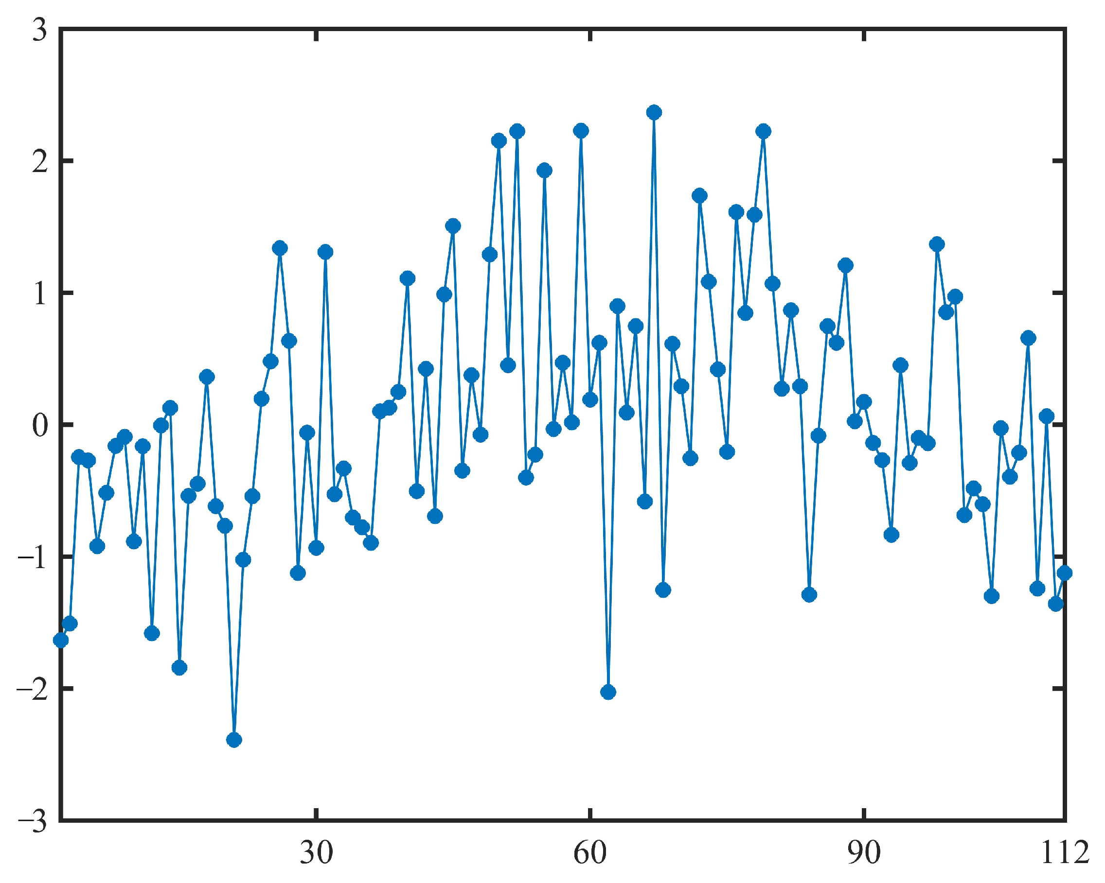
By substituting the estimated m ^ , a ^ , and σ ^ into (22), we can obtain 111 samples h 2 , h 3 , , h 112 of the normal uncertainty distribution N ( 0 , 1 ) , as shown in Table 7 and Figure 6.
If the estimated parameters m ^ , a ^ , and σ ^ are appropriate, then the obtained h 2 , h 3 , , h 112 should indeed be a set of samples of normal uncertainty distribution N ( 0 , 1 ) . That is, the test of the estimated parameters m ^ , a ^ , and σ ^ is equivalent to testing whether h 2 , h 3 , , h 112 is a set of samples of N ( 0 , 1 ) , whose test for a given significance level α = 0.01 is
W = { ( h 2 , h 3 , , h 112 ) : there   are   at   least   2   of   indexes   i s   with   2 i 112 such   that   h i < Φ 1 α 2   or   h i > Φ 1 1 α 2 ,
where
Φ 1 α = 3 π ln α 1 α
is the inverse uncertainty distribution of N ( 0 , 1 ) . As shown in Table 7 and Figure 6, it is easy to see that all the points in h 2 , h 3 , , h 112 are within the interval
Φ 1 α 2 , Φ 1 1 α 2 = [ 2.9184 , 2.9184 ] .
Thus, we obtain
( h 2 , h 3 , , h 112 ) W .
That is, the obtained h 2 , h 3 , , h 112 is indeed a set of samples of normal uncertainty distribution N ( 0 , 1 ) . Therefore, the estimated parameters m ^ , a ^ , and σ ^ are appropriate.

8.3. Stochastic Stock Prices Model

In this subsection, we retain the closing prices of Anhui Gujinggong Liquor Co., Ltd. from 1 January 2024 to 21 June 2024 shown in Table 6 and Figure 5, as described in the previous subsection, and choose the following stochastic mean reversion equation:
d X t = ( m a X t ) d t + σ d W t ,
to model the closing prices x i , i = 1 , 2 , , 112 , where W t is a Wiener process.
Before modeling the closing prices, we first derive the statistical invariant based on the above stochastic mean reversion equation. By writing the above stochastic mean reversion equation into the Euler difference form, we obtain
X i = X i 1 + ( m a X i 1 ) + σ ( W i W i 1 ) , i = 2 , 3 , , 112 .
Based on the above Euler difference form, we can obtain
X i X i 1 ( m a X i 1 ) σ = W i W i 1 , i = 2 , 3 , , 112 ,
which are independent and identically distributed standard normal random variables according to the definition of the Wiener process and its property of independent increments. That is, we have
X i X i 1 ( m a X i 1 ) σ = W i W i 1 N ( 0 , 1 ) .
We substitute the closing prices x i , i = 1 , 2 , , 112 into X i X i 1 ( m a X i 1 ) σ and write
h i ( m , a , σ ) = x i x i 1 m + a x i 1 σ , i = 2 , 3 , , 112 ,
which are a set of samples of the standard normal random distribution function N ( 0 , 1 ) .
Similar to the least squares estimation based on the uncertainty distribution, we can also derive that the least squares estimation of ( m , a , σ ) based on the random distribution function is the solution to the optimization problem,
min m , a , σ i = 2 112 Ψ x i x i 1 m + a x i 1 σ 1 111 j = 2 112 I x j x j 1 + a x j 1 x i x i 1 + a x i 1 2 ,
where Ψ is the random distribution function of the standard normal random distribution function N ( 0 , 1 ) . By using MATLAB to solve the above minimization problem, the optimal solution can be obtained as
m ^ = 36.3820 , a ^ = 0.1529 , σ ^ = 5.4680 .
Thus, the estimated stochastic stock prices model is
d X t = ( 36.3820 0.1529 X t ) d t + 5.4680 d W t .
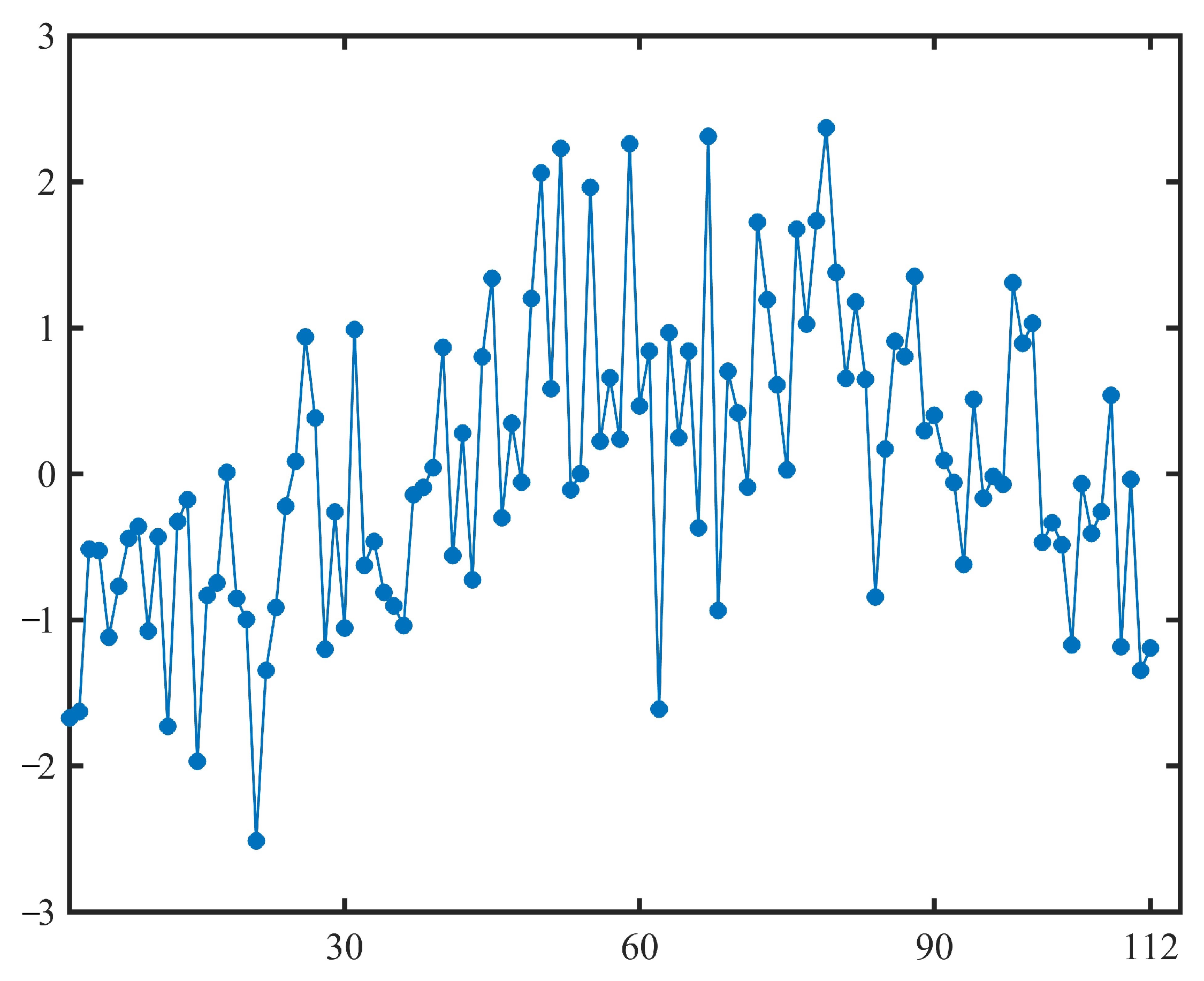
By substituting the estimated m ^ , a ^ , and σ ^ into (24), we can obtain 111 samples h 2 , h 3 , , h 112 of the standard normal random distribution function N ( 0 , 1 ) , as shown in Table 8 and Figure 7.
As shown in Table 8 and Figure 7, if we select two non-overlapping parts from the 111 samples of the standard normal random distribution function N ( 0 , 1 ) , i.e.,
h 2 , h 3 , , h 30
and
h 62 , h 63 , , h 90 ,
and use the two-sample Kolmogorov–Smirnov test to test them via the function “kstest2” in MATLAB, then the p value is 1.4798 × 10 7 , which shows that the above two parts do not come from the same population. Thus, the samples h 2 , h 3 , , h n 112 are not white noise in the sense of probability theory, nor do they follow the standard normal random distribution function N ( 0 , 1 ) . Thus, the least squares estimation based on the uncertainty distribution for uncertain differential equations is more appropriate than the least squares estimation based on the random distribution function for stochastic differential equations.

9. Conclusions

For the purpose of overcoming the disadvantage that the current parameter estimation study of uncertain differential equations is strictly dependent on the solvability of residuals and cannot be applied to general uncertain differential equations, a symmetrical statistical invariant based on the difference scheme of uncertain differential equations was constructed. Further, based on the statistical invariant and the principle of least squares, the least squares estimation for the fixed constant parameters and time-varying parameters of the uncertain differential equations were investigated, and the corresponding numerical solutions were also designed to facilitate the acquisition of the numerical solution of the above least squares estimations. Finally, two numerical examples and an empirical study were provided to illustrate the effects of the methods proposed in this paper.

Author Contributions

Conceptualization, X.X.; methodology, X.X. and Y.D.; software, X.X.; validation, X.X. and Y.D.; formal analysis, Y.D.; investigation, X.X.; resources, X.X. and Y.D.; data curation, X.X.; writing—original draft preparation, X.X.; writing—review and editing, Y.D.; supervision, X.X. and Y.D. All authors have read and agreed to the published version of the manuscript.

Funding

This research received no external funding.

Data Availability Statement

The original contributions presented in this study are included in the article, and the research data mentioned in this article have been presented in Table 1, Table 3 and Table 6. Further inquiries can be directed to the corresponding author.

Acknowledgments

The authors especially thank the editors and anonymous referees for their kindly review and helpful comments. Any remaining errors are ours.

Conflicts of Interest

We declare that we have no relevant or material financial interests that relate to the research described in this paper. Neither the entire paper nor any part of its content has been published or accepted elsewhere. It is also not being submitted to any other journal.

References

  1. Kolmogorov, A. Grundbegriffe der Wahrscheinlichkeitsrechnung; Springer: Berlin/Heidelberg, Germany, 1933. [Google Scholar]
  2. Liu, B. Uncertainty Theory, 2nd ed.; Springer: Berlin/Heidelberg, Germany, 2007. [Google Scholar]
  3. Yang, X.; Ke, H. Uncertain interest rate model for Shanghai interbank offered rate and pricing of American swaption. Fuzzy Optim. Decis. Mak. 2023, 22, 447–462. [Google Scholar] [CrossRef]
  4. Yang, L.; Liu, Y. Solution method and parameter estimation of uncertain partial differential equation with application to China’s population. Fuzzy Optim. Decis. Mak. 2024, 23, 155–177. [Google Scholar] [CrossRef]
  5. Liu, Y.; Qin, Z.; Li, X. Are the queueing systems in practice random or uncertain? Evidence from online car-hailing data in Beijing. Fuzzy Optim. Decis. Mak. 2024, 23, 497–511. [Google Scholar] [CrossRef]
  6. Liu, B. Uncertainty Theory, 5th ed.; Springer: Berlin/Heidelberg, Germany, 2025; Available online: https://cloud.tsinghua.edu.cn/d/df71e9ec330e49e59c9c/files/?p=%2FUncertainty.Theory.Book.pdf (accessed on 19 September 2025).
  7. Yao, K. Uncertain Differential Equations; Springer: Berlin/Heidelberg, Germany, 2016. [Google Scholar]
  8. Zhu, Y. Uncertain Optimal Control; Springer: Singapore, 2019. [Google Scholar]
  9. Yao, K. Uncertain Renewal Processes; Springer: Singapore, 2019. [Google Scholar]
  10. Zhang, B.; Peng, J. Uncertain Graph and Network Optimization; Springer: Singapore, 2022. [Google Scholar]
  11. Liu, B. Fuzzy process, hybrid process and uncertain process. J. Uncertain Syst. 2008, 2, 3–16. [Google Scholar]
  12. Chen, X.; Liu, B. Existence and uniqueness theorem for uncertain differential equations. Fuzzy Optim. Decis. Mak. 2010, 9, 69–81. [Google Scholar] [CrossRef]
  13. Liu, B. Some research problems in uncertainty theory. J. Uncertain Syst. 2009, 3, 3–10. [Google Scholar]
  14. Yao, K.; Gao, J.; Gao, Y. Some stability theorems of uncertain differential equation. Fuzzy Optim. Decis. Mak. 2013, 12, 3–13. [Google Scholar] [CrossRef]
  15. Yao, K.; Chen, X. A numerical method for solving uncertain differential equations. J. Intell. Fuzzy Syst. 2013, 25, 825–832. [Google Scholar] [CrossRef]
  16. Yao, K.; Liu, B. Parameter estimation in uncertain differential equations. Fuzzy Optim. Decis. Mak. 2020, 19, 1–12. [Google Scholar] [CrossRef]
  17. Liu, Z. Generalized moment estimation for uncertain differential equations. Appl. Math. Comput. 2021, 392, 125724. [Google Scholar] [CrossRef]
  18. Sheng, Y.; Yao, K.; Chen, X. Least squares estimation in uncertain differential equations. IEEE Trans. Fuzzy Syst. 2020, 28, 2651–2655. [Google Scholar] [CrossRef]
  19. Yang, X.; Liu, Y.H.; Park, G. Parameter estimation of uncertain differential equation with application to financial market. Chaos Solitons Fract. 2020, 139, 110026. [Google Scholar] [CrossRef]
  20. Liu, Y.; Liu, B. Estimating unknown parameters in uncertain differential equation by maximum likelihood estimation. Soft Comput. 2022, 26, 2773–2780. [Google Scholar] [CrossRef]
  21. Liu, Y.; Liu, B. Residual analysis and parameter estimation of uncertain differential equations. Fuzzy Optim. Decis. Mak. 2022, 21, 513–530. [Google Scholar] [CrossRef]
  22. Liu, Y.; Liu, B. A modified uncertain maximum likelihood estimation with applications in uncertain statistics. Commun. Stat.—Theory Methods 2024, 53, 6649–6670. [Google Scholar] [CrossRef]
  23. Liu, Y.; Liu, B. Estimation of uncertainty distribution function by the principle of least squares. Commun. Stat.—Theory Methods 2024, 53, 7624–7641. [Google Scholar] [CrossRef]
  24. Yao, L.; Sheng, Y. Moments estimation for multi-factor uncertain differential equations based on residuals. Soft Comput. 2023, 27, 11193–11203. [Google Scholar] [CrossRef]
  25. Liu, Z.; Liu, Y.; Gao, R. Maximum likelihood estimation for multi-factor uncertain differential equations. J. Comput. Appl. Math. 2025, 454, 116205. [Google Scholar] [CrossRef]
  26. Wu, N.; Liu, Y. Least squares estimation of multifactor uncertain differential equations with applications to the stock market. Symmetry 2024, 16, 904. [Google Scholar] [CrossRef]
  27. Yang, L.; Liu, Y. Least squares estimation of uncertain partial differential equations. Math. Method. Appl. Sci. 2025, 48, 3482–3495. [Google Scholar] [CrossRef]
  28. Ye, T.; Liu, B. Uncertain hypothesis test with application to uncertain regression analysis. Fuzzy Optim. Decis. Mak. 2022, 21, 157–174. [Google Scholar] [CrossRef]
Figure 1. The samples of normal uncertainty distribution N ( 0 , 1 ) obtained in Example 2.
Symmetry 17 01594 g001
Figure 2. The estimated μ ^ t j with t j , j = 1 , 2 , , 100 in Example 3.
Symmetry 17 01594 g002
Figure 3. The estimated σ ^ t j with t j , j = 1 , 2 , , 100 in Example 3.
Symmetry 17 01594 g003
Figure 4. The samples of normal uncertainty distribution N ( 0 , 1 ) obtained in Example 3.
Symmetry 17 01594 g004
Figure 5. The closing prices of Anhui Gujinggong Liquor Co., Ltd. from 1 January 2024 to 21 June 2024 accessed by Sina Finance https://finance.sina.com.cn/realstock/company/sz000596/nc.shtml (accessed on 12 September 2025).
Symmetry 17 01594 g005
Figure 6. The samples of normal uncertainty distribution N ( 0 , 1 ) obtained in uncertain stock prices model (23).
Symmetry 17 01594 g006
Figure 7. The samples of the standard normal random distribution function N ( 0 , 1 ) obtained in stochastic stock prices model (25).
Symmetry 17 01594 g007
Table 1. Observational data in Example 2.
t i x t i t i x t i t i x t i t i x t i
0.1784−2.10822.36770.69975.08513.18397.53214.8684
0.3556−1.98322.50700.85635.32623.26927.59464.9250
0.4238−1.86492.83551.07405.41793.36697.88155.0983
0.6345−1.57152.92971.24005.72853.75318.17755.4798
1.0840−1.04783.23641.47036.03103.91688.36595.6311
1.2637−0.82643.58881.90346.22054.03138.60055.9770
1.6510−0.15713.86252.01816.60524.17348.98396.5978
1.97100.30003.95432.15356.78234.34939.37216.7845
2.09550.46244.32822.40316.89634.44089.45266.8835
2.16230.48814.39762.43756.96334.5117
2.26160.59464.71492.91087.05614.5659
2.31720.65495.00743.13387.27044.7023
Table 2. The samples of normal uncertainty distribution N ( 0 , 1 ) obtained in Example 2.
−0.46101.55320.88620.43940.57111.54310.95590.7106−1.0881
0.26060.2793−0.10190.3590−0.54461.6123−0.37160.5653−1.0215
1.0445−0.5350−0.87201.0799−0.3492−0.5799−1.14940.24440.5937
−0.7826−0.6585−1.11930.1048−0.27210.2308−0.6980−0.5956−0.5991
−0.0716−0.65890.6814−0.26881.04591.3292−0.90000.5638
Table 3. Observational data in Example 3.
t i x t i t i x t i t i x t i t i x t i
0.03200.09311.52240.26142.97070.60734.11760.9295
0.13950.10091.62240.28602.98670.61594.17160.9777
0.21160.10651.65490.29343.00800.62554.19130.9738
0.29640.11381.70400.30243.02590.63284.29731.0292
0.32190.11611.72610.30413.03730.63494.30851.0315
0.35080.11861.74750.30703.06570.63704.36661.0360
0.42170.12501.86550.31643.08730.64364.37901.0463
0.46130.12861.91250.33073.11440.64444.43651.0874
0.53530.13631.95750.33513.19790.64254.50641.0467
0.57060.13951.98590.33823.25320.64204.67581.0420
0.58360.14082.06290.36593.27570.64204.76361.0228
0.61500.14422.18000.38833.30670.64744.78781.0249
0.62990.14592.20620.39113.34850.67894.80381.0257
0.64350.14762.26390.39793.36810.68134.84091.0516
0.74300.15922.29620.40143.43950.70164.86631.0582
0.78870.16392.34200.40843.51050.72644.91281.0196
0.84310.17082.36280.41563.52210.73124.92321.0250
0.90150.17702.37470.42103.55420.74354.96551.0038
0.94390.18132.45300.44353.58910.77714.98871.0294
1.02100.18902.51390.47243.65180.81655.01341.0285
1.08320.19652.57310.47713.70190.81485.03951.0602
1.12970.20202.60750.48413.73410.84235.08801.0946
1.17550.20582.63750.49143.77420.86245.12961.1411
1.18750.20812.66260.49333.80500.86345.15131.1391
1.21790.21172.71970.50403.88390.88385.19371.1208
1.25570.21672.74000.51173.93500.89185.25111.1385
1.31120.22552.82960.55493.97000.93355.30771.0958
1.35600.23192.84220.55443.99410.94245.31871.1050
1.37930.23582.89260.56634.01100.94175.40711.1002
1.45510.24682.90410.57064.05680.92735.43291.1186
Table 4. The estimated μ ^ t j and σ ^ t j with j = 1 , 2 , , 100 in Example 3.
μ t j σ t j μ t j σ t j μ t j σ t j μ t j σ t j
0.73540.09540.61580.29420.48970.37720.38100.4458
0.72130.11110.60910.29690.51410.41650.38270.4527
0.70640.12700.60490.31090.54990.41180.37480.4369
0.70800.13270.56750.31220.57830.39240.33000.4316
0.69320.14130.54810.33710.57900.39080.33100.4313
0.68210.14270.52770.34250.56800.41520.33430.4248
0.68080.14010.53270.35340.54020.39680.35780.4808
0.67310.14060.55180.39000.48740.39670.38060.4555
0.66900.13080.54840.38530.44250.42380.38030.4565
0.66490.13500.57230.42480.38790.41420.37570.4818
0.67050.14880.52380.42000.38110.43110.37690.4771
0.67460.16050.48500.37060.36660.43230.42490.5407
0.67550.16260.45620.31330.38830.47910.35500.5222
0.66010.14330.41640.28850.38970.47650.38620.5257
0.64150.13930.42170.27240.39350.47730.36730.5317
0.63230.16060.45880.35400.37740.45030.33270.5401
0.61210.16560.50810.40260.36470.41880.34670.5691
0.62440.20070.45210.37840.40270.38880.35900.5886
0.61390.23300.46090.36870.43040.43870.27780.5731
0.60170.26390.49050.38070.43800.45530.21950.5328
Table 5. The samples of normal uncertainty distribution N ( 0 , 1 ) obtained in Example 3.
0.28870.24860.62260.43670.29680.35720.17480.7016−0.0654
0.27300.51560.59070.98890.6417−0.00530.6515−0.1051−0.2377
−0.30430.1318−0.0391−0.70731.2839−0.07640.12710.58020.2210
0.55540.17181.11141.30880.84980.3145−0.8332−0.2165−0.7801
1.3694−0.5808−0.46251.64140.1351−0.4722−0.3969−0.4480−0.1641
1.05341.66310.62351.5862−0.58630.05380.2453−0.5593−0.0336
0.82641.2629−0.94260.12130.64041.31491.12980.80470.6414
−0.1174−0.46550.2891−0.6024−0.7542−0.6718−0.6198−0.07491.6776
−0.23470.23060.39920.54370.46531.89350.9971−0.55011.4302
0.6127−0.35980.1038−0.08751.90750.3020−0.4414−0.9219−0.2796
1.2611−0.64540.56860.0511−0.15510.99980.8180−1.0748−0.2652
−0.4971−0.0400−0.08420.83850.2111−1.27520.5928−0.82691.4410
−0.16731.55910.83241.3284−0.1970−0.60500.3042−0.96140.9620
−0.11540.8258
Table 6. The closing prices of Anhui Gujinggong Liquor Co., Ltd. from 1 January 2024 to 21 June 2024, accessed by Sina Finance https://finance.sina.com.cn/realstock/company/sz000596/nc.shtml (accessed on 12 September 2025).
224.34217.28211.55212.77213.75211.34211.21212.89214.76
212.43213.98208.2210.97214.14207.02207.2207.83212.5
211.74210.3200.79199.12200.06204.65210.22219.6224.5
220221.33218.11226.56224.88224.36222219.5216.65
219.13221.51224.26231.1229.1231.99228.94234.7242.53
240.19241.75240.87247256.89257.19266.45261.5257.92
265.6262.6262.44260269266.8267253.76256.64
255.15257.13252.18262.65253.76255.19254.85251.78259.1
262.39261.99258.47264.5266.06271.24279.12280.38277.48
277.88275.32265261.8263.13263.68267.15264.3262.47
259.24255.67249.58250.6247.77246.18244.54250.7253.65
256.9251.45247.56243.44236.2236.11234.17233.34237
230.68231.59225.21220.64
Table 7. The samples of normal uncertainty distribution N ( 0 , 1 ) obtained in uncertain stock prices model (23).
−1.6333−1.5074−0.2465−0.2703−0.9204−0.5170−0.1623−0.0923−0.8851
−0.1644−1.5811−0.00540.1271−1.8425−0.5395−0.44720.3624−0.6189
−0.7679−2.3886−1.0252−0.54230.19630.47851.33830.6356−1.1249
−0.0613−0.93361.3074−0.5285−0.3320−0.7052−0.7785−0.89600.1009
0.12910.24821.1087−0.50380.4227−0.69380.98611.5061−0.3497
0.3748−0.07661.29002.15070.44932.2236−0.4020−0.22731.9258
−0.03350.46900.01592.22660.19020.6213−2.02760.89790.0911
0.7472−0.58232.3654−1.25320.61170.2901−0.25541.73601.0822
0.4175−0.20601.61080.84521.58992.22311.06890.27220.8674
0.2910−1.2902−0.08460.74760.61941.20630.02610.1723−0.1395
−0.2691−0.83560.4499−0.2902−0.1003−0.14091.36690.85250.9688
−0.6854−0.4830−0.6037−1.2992−0.0281−0.3950−0.21340.6567−1.2423
0.0625−1.3588−1.1250
Table 8. The samples of the standard normal random distribution function N ( 0 , 1 ) obtained in stochastic stock prices model (25).
−1.6729−1.6271−0.5162−0.5260−1.1186−0.7690−0.4416−0.3599−1.0757
−0.4313−1.7285−0.3264−0.1758−1.9691−0.8331−0.74570.0107−0.8518
−0.9974−2.5135−1.3456−0.9149−0.22110.08640.93890.3819−1.2003
−0.2599−1.05480.9894−0.6269−0.4618−0.8128−0.9044−1.0383−0.1432
−0.09220.04200.8669−0.55850.2798−0.72570.80031.3399−0.3012
0.3467−0.05601.20142.06050.58312.2301−0.10980.00241.9616
0.22310.65860.23722.26110.46450.8419−1.61050.96740.2488
0.8417−0.37032.3114−0.93660.70230.4185−0.09021.72411.1917
0.60890.02711.67521.02631.73192.37061.38020.65461.1770
0.6469−0.84390.16970.90870.80331.35270.29390.40070.0935
−0.0590−0.61960.5104−0.1652−0.0175−0.07111.30950.89471.0320
−0.4682−0.3353−0.4861−1.1719−0.0667−0.4075−0.25870.5392−1.1837
−0.0381−1.3459−1.1932
Disclaimer/Publisher’s Note: The statements, opinions and data contained in all publications are solely those of the individual author(s) and contributor(s) and not of MDPI and/or the editor(s). MDPI and/or the editor(s) disclaim responsibility for any injury to people or property resulting from any ideas, methods, instructions or products referred to in the content.