The One-Fault Dimension-Balanced Hamiltonian Problem in Toroidal Mesh Graphs

Abstract

Finding a Hamiltonian cycle in a graph G = (V, E) is a well-known problem. The challenge of finding a Hamiltonian cycle that avoids these faults when faulty vertices or edges are present has been extensively studied. When the edge set of G is partitioned into k dimensions, the problem of dimension-balanced Hamiltonian cycles arises, where the Hamiltonian cycle uses approximately the same number of edges from each dimension (differing by at most one). This paper studies whether a dimension-balanced Hamiltonian cycle (DBH) exists in toroidal mesh graphs T_m,n when a single vertex or edge is faulty, called the one-fault DBH problem. We establish that T_m,n is one-fault DBH, except in the following cases: (1) both m and n are even; (2) one of m and n is 3, while the other satisfies mod 4 = 3 and is greater than 6; (3) one of m and n is odd, while the other satisfies mod 4 = 2. Additionally, this paper resolves a conjecture from prior literature, thereby providing a complete solution to the DBP problem on T_m,n.

1. Introduction

With the widespread use of networks today, we can represent the topological structure of the network with graphs, where vertices represent devices, and edges between vertices represent communication between those devices. The connection paths between vertices in the graph can show the network’s operational efficiency, where a Hamiltonian cycle can connect all the vertices and return to the original vertex, ensuring the network remains smooth. The Hamilton problem is a famous problem in interconnection networks [1,2,3,4,5]. However, when some vertices or edges fail, the Hamiltonian cycle is disrupted, causing data transmission issues. This inconvenience requires new routes for data transmission to be ensured in the network. Therefore, scholars have further discussed Hamiltonian cycles, particularly whether Hamiltonian cycles still exist in network graphs when there are faulty vertices or edges [6,7,8,9,10,11,12,13,14,15].

Given a graph G = (V, E) whose edge set E(G) is partitioned into k dimensions (E = E₁ ∪ E₂ ∪ … ∪ E_k), a cycle C in G for i with 1 ≤ i ≤ k has edges in i-dimension E_i(C), defined as E(C) ∩ E_i. A cycle C is called a dimension-balanced cycle (DBC for short) if ∣∣E_i(C)∣ − ∣E_j(C)∣∣ ≤ 1 for all i and j with 1 ≤ i < j ≤ k. If C is also a Hamiltonian cycle (passing through all vertices in the graph), it is called a dimension-balanced Hamiltonian cycle (DBH for short). If G contains a DBC of every length between 3 and |V|, G is called dimension-balanced pancyclic (DBP for short). If G contains a DBC of every length between a and |V(G)|, G is called dimension-balanced a-pancyclic (a-DBP). If for any vertex x in G there exists a DBC containing x whose length can be any integer between a and |V(G)|, G is called dimension-balanced a-vertex-pancyclic (a-DBVP). Moreover, a cycle C is called a weakly dimension-balanced cycle (WDBC for short) if ∣∣E_i(C)∣ − ∣E_j(C)∣∣ ≤ 3 for all i and j with 1 ≤ i < j ≤ k. If C is also a Hamiltonian cycle, it is called a weakly dimension-balanced Hamiltonian cycle (WDBH for short). Similarly, if G contains a WDBC of every length between 3 and |V|, G is called weakly dimension-balanced pancyclic (WDBP for short).

A cycle C_n with n vertices forms a toroidal mesh graph T_m,n when taking the Cartesian product of C_m and C_n. It is defined as follows: vertex set V(T_m,n) = {(x, y) ∣ 0 ≤ x ≤ m − 1; 0 ≤ y ≤ n − 1}, and edge set E(T_m,n) = {(x₁, y₁)(x₂, y₂) ∣ x₁ = x₂ and ∣y₁ − y₂∣ = (1 or n − 1) or ∣x₁ − x₂∣ = (1 or m − 1) and y₁ = y₂}. Figure 1 shows an example of T_4,3. The toroidal mesh graph is an important interconnection network graph. We partition its edges into two sets: horizontal edges and vertical edges. Thus, E(T_m,n) = E₁ ∪ E₂, where E₁ = {(i, j)(i + 1, j) ∣ 0 ≤ i ≤ m − 2; 0 ≤ j ≤ n − 1} ∪ {(m − 1, j)(0, j) ∣ 0 ≤ j ≤ n − 1} and E₂ = {(i, j)(i, j + 1) ∣ 0 ≤ i ≤ m − 1; 0 ≤ j ≤ n − 2} ∪ {(i, n − 1)(i, 0) ∣ 0 ≤ i ≤ m − 1}. This paper’s research is based on this partition.

The dimension-balanced Hamiltonian problem was first proposed in 2012 [16], and originated from the 3D reconstruction problem using Gray codes [17]. It has been widely explored since then [18,19,20,21]: the authors of [16] first studied the DBH problem on T_m,n, and the DBP problem on T_m,n was solved [18]. Subsequently, the extension problem known as the WDBH problem was raised, and the WDBH problem on T_m,n was solved in [19], and then, the WDBP problem was also studied [20]. In addition, [21] conducted research on the DBH problem on a 3-Dimensional Toroidal Mesh Graph T_m,n,r.

The design of the network-on-chip (NoC) has become a significant research focus in recent years. Congestion in the NoC can lead to a decline in network performance. Therefore, the efficient selection of paths and the development of effective strategies to address congestion are critical for optimizing NoC performance. This topic has attracted considerable attention in recent studies [22,23]. Through abstraction, some NoCs can be represented as a toroidal mesh graph. A dimension-balanced Hamiltonian cycle on a toroidal mesh graph provides a foundation for designing simple algorithms with low communication costs, effectively mitigating congestion. In addition to being used to assist in the design of NoC, toroidal mesh graphs are also very helpful for research in fields such as cryptography and graphics. The dimension-balanced Hamiltonian cycle problem in toroidal mesh graphs has been discussed in [16]. The question of whether a dimension-balanced Hamiltonian cycle exists for toroidal mesh graphs T_m,n has been thoroughly discussed. This paper focuses on the problem of dimension-balanced Hamiltonian cycles in toroidal mesh graphs with a faulty point f or faulty edge e.

A graph G is called k-node Hamiltonian if it remains Hamiltonian after removing any k-nodes; a graph G is called k-edge (or say k-link) Hamiltonian if it remains Hamiltonian after removing any k edges (links); G is called k-fault Hamiltonian if it remains Hamiltonian after removing any k-nodes and/or edges [5,6]. In recent years, many researchers have studied the Hamiltonian problem on several topologies with faulty nodes or edges, like Cartesian product graphs [8,11], locally twisted cubes [10], augmented cubes [7,12], hypercube graphs [13], the basic WK-recursive pyramid [14], and so on. This gives us strong motivation to study DBC problems with faulty nodes or edges.

Therefore, we have the following definitions which define a dimension-balanced Hamiltonian on a graph G with faulty nodes and/or edges. A graph G is called k-node dimension-balanced Hamiltonian (k-node DBH for short) if it has a DBH after removing any k-nodes; a graph G is called k-edge dimension-balanced Hamiltonian (k-edge DBH for short) if it remains Hamiltonian after removing any k edges; a graph G is called k-fault dimension-balanced Hamiltonian (k-fault DBH for short) if it remains Hamiltonian after removing any k-nodes and/or edges.

This paper mainly discusses under what conditions a toroidal mesh graph is one-fault dimension-balanced Hamiltonian. The main contributions of this paper are as follows:

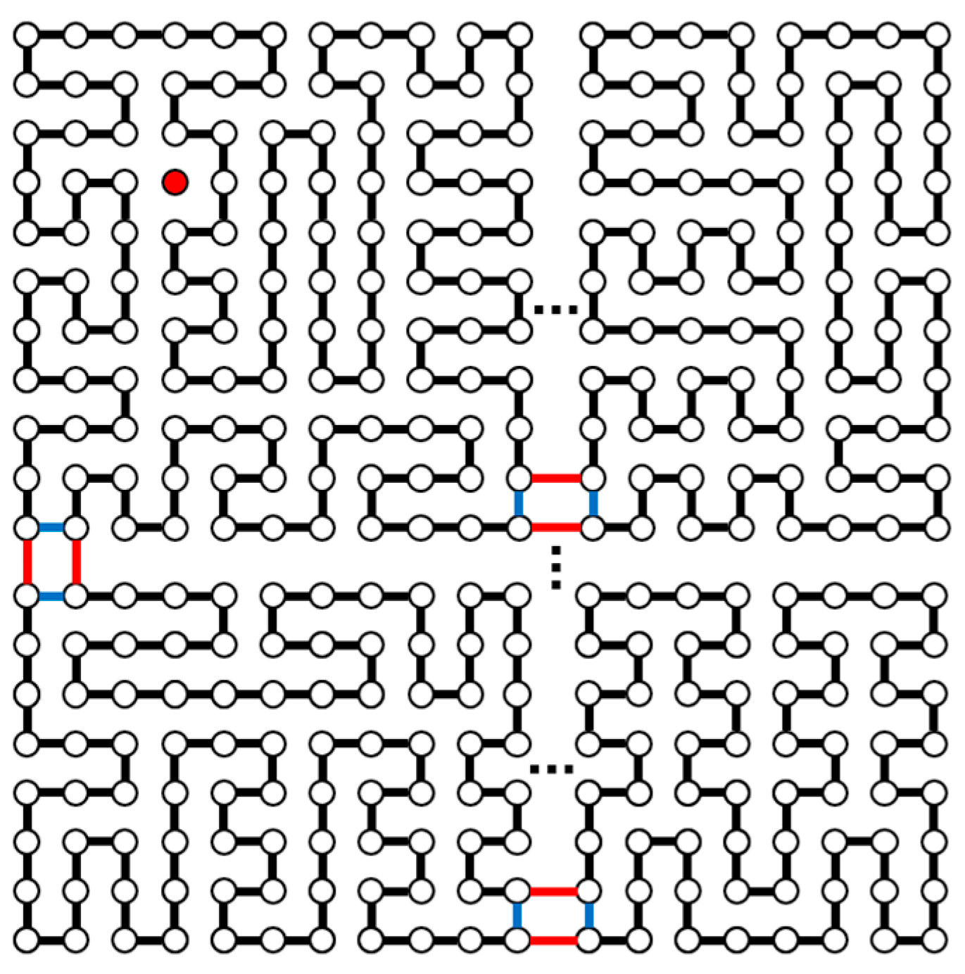
• We completely solve the one-fault dimension-balanced Hamiltonian problem on the toroidal mesh graph T_m,n.
• We prove the three conjectures in [18]: when m and n ≥ 5 are both odd numbers, for k = ⌊(mn − 1) / 4⌋, there is a DBC of length 4k in T_m,n; therefore, T_m,n is (2 max{m, n} − 1)-DBP and (2 max{m, n} − 1)-DBVP.

The rest of this paper is organized as follows. In Section 2, the problem of finding dimension-balanced Hamiltonian cycles in T_m,n − f is discussed. According to the parity of m and n, there are three subsections: both m and n are even; both m and n are odd; one of m and n is even and the other is odd. Section 3 illustrate the problem in T_m,n − e and presents our conclusions.

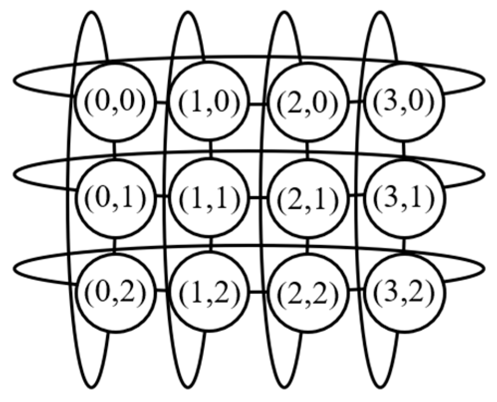
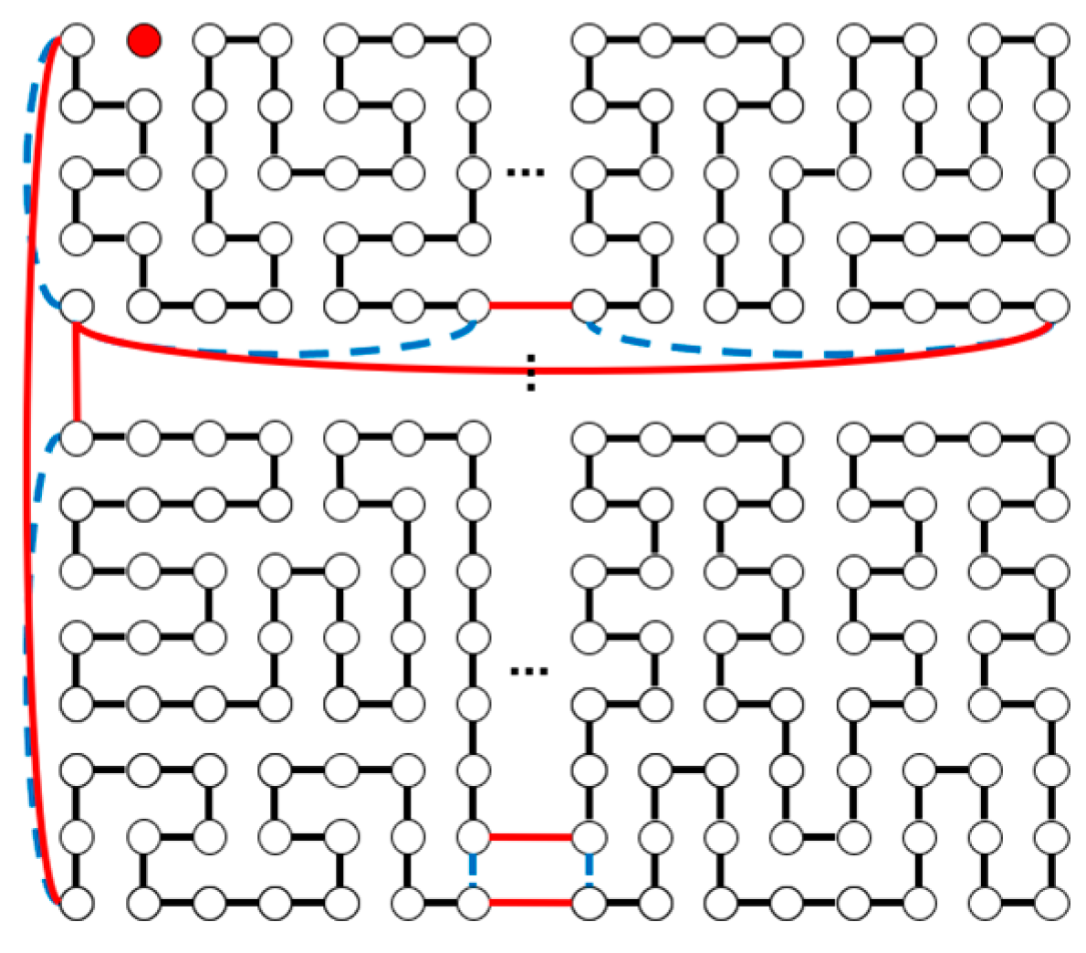
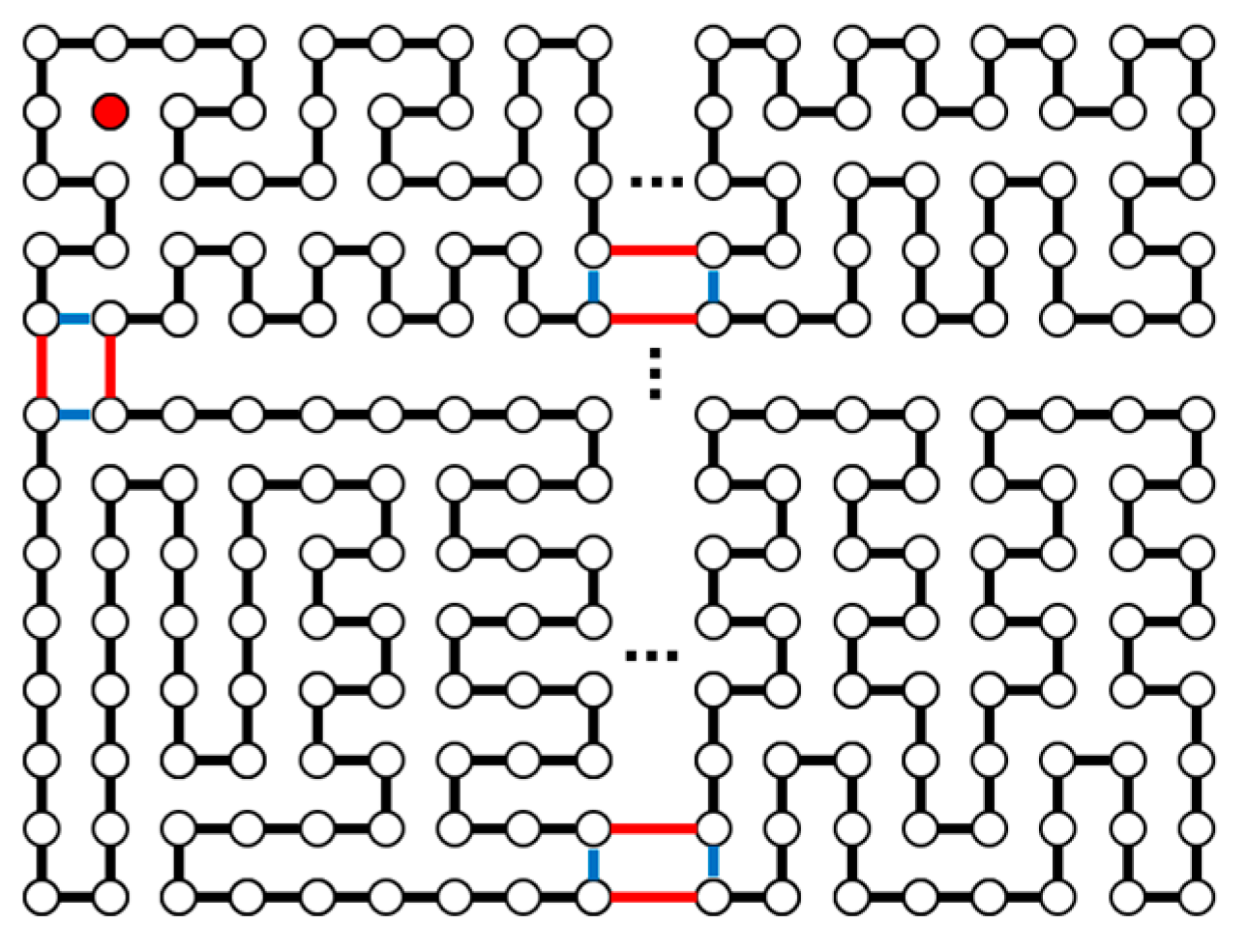
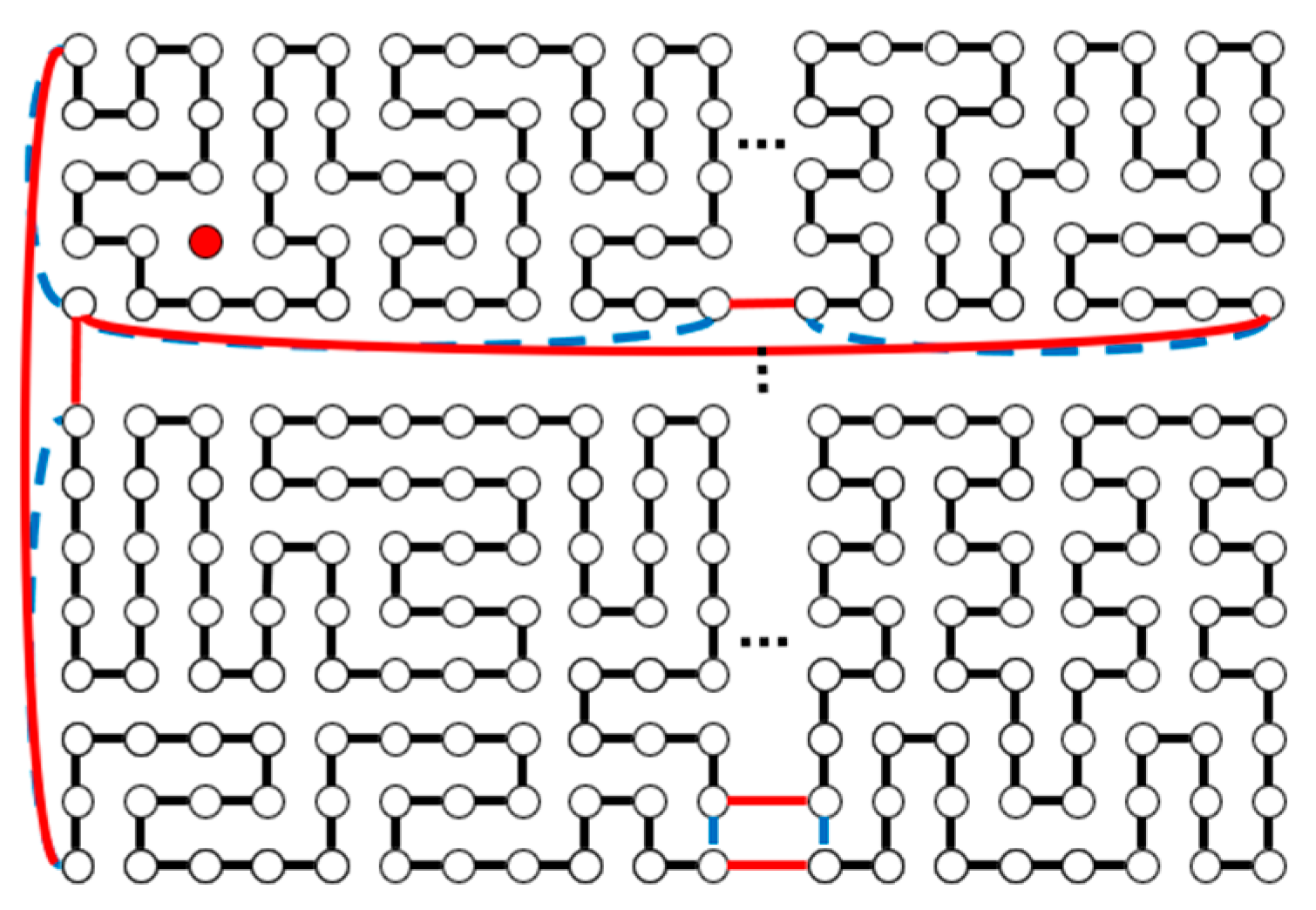
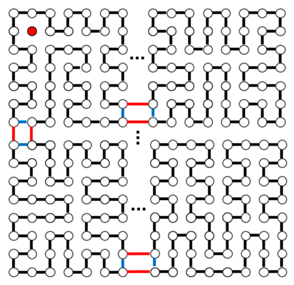
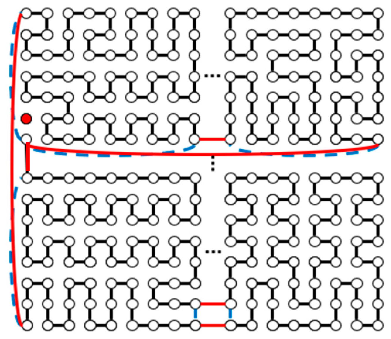
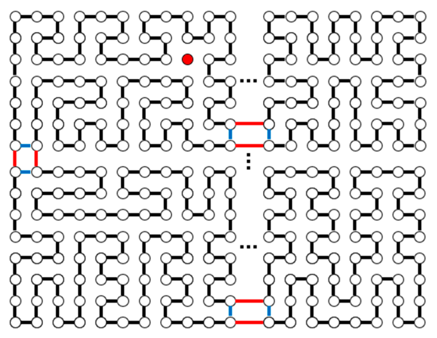
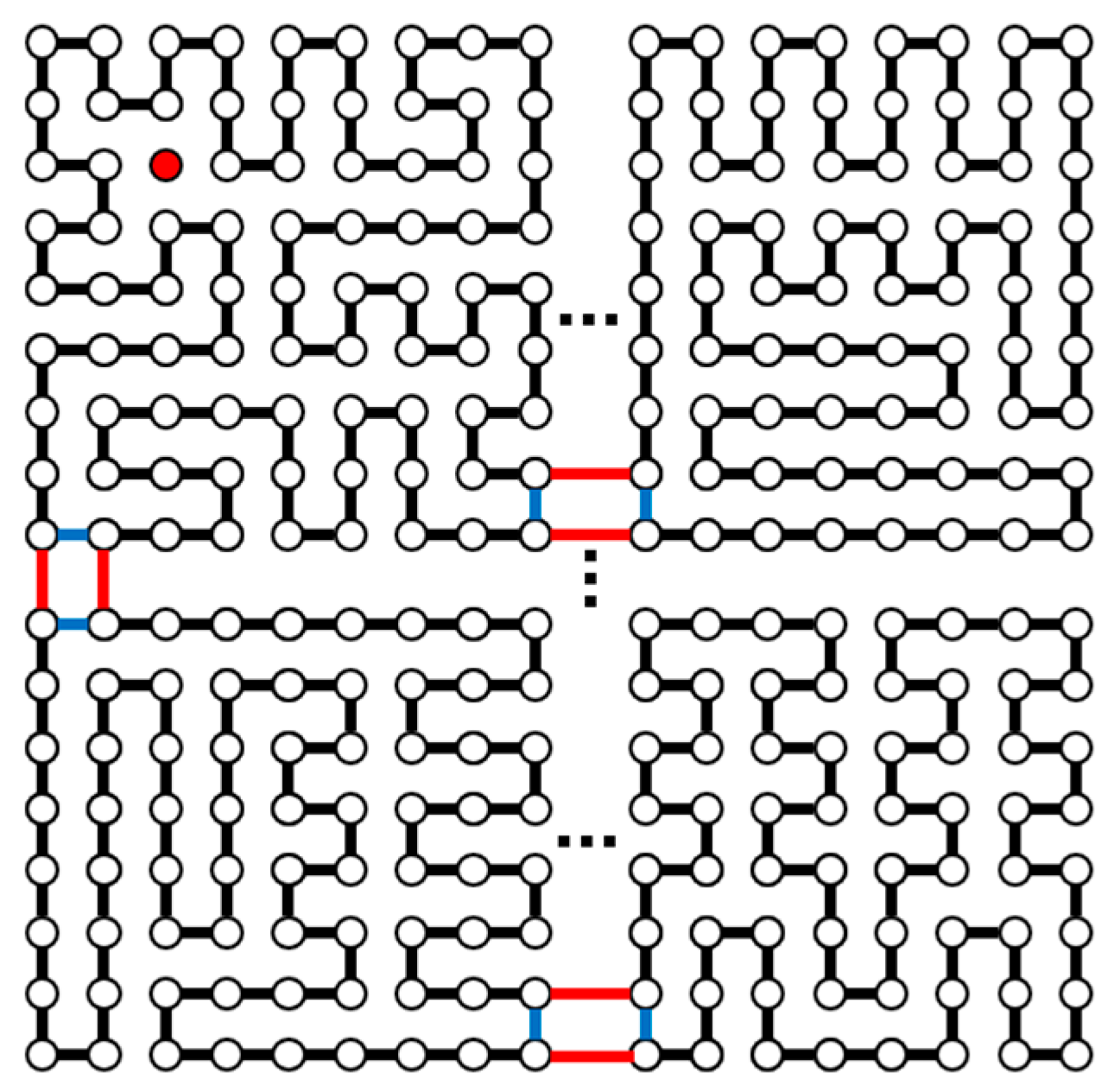
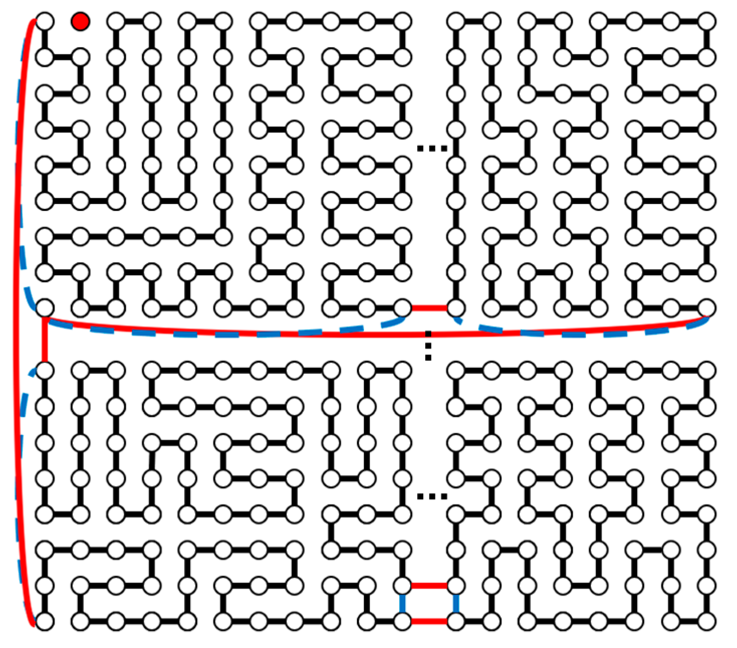
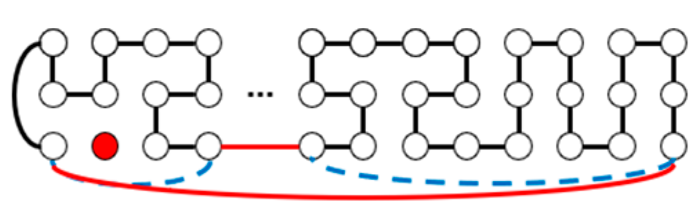
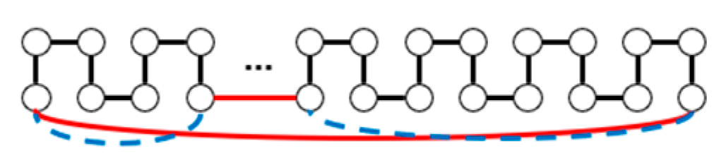
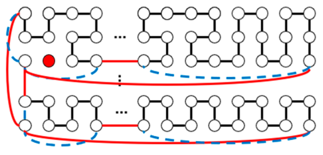
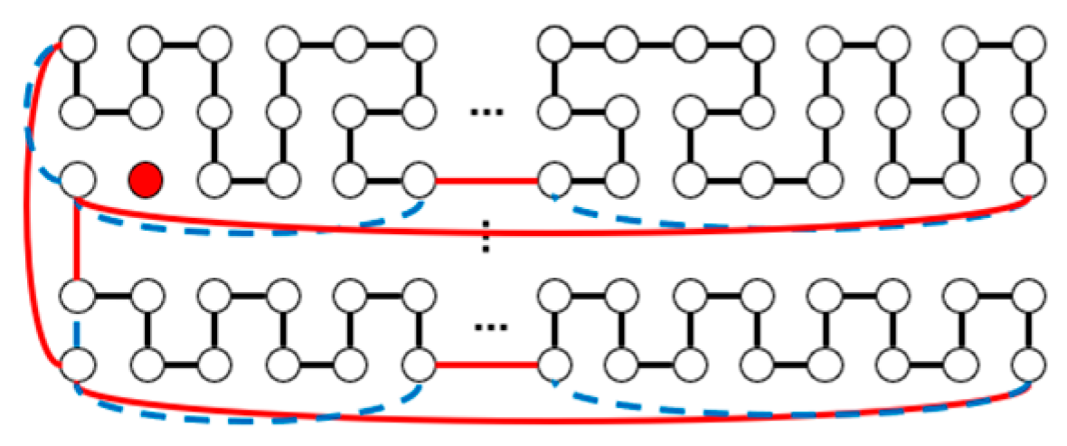
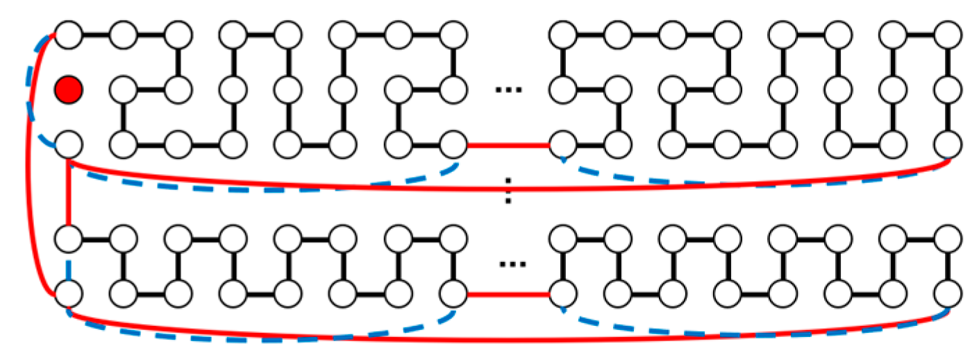
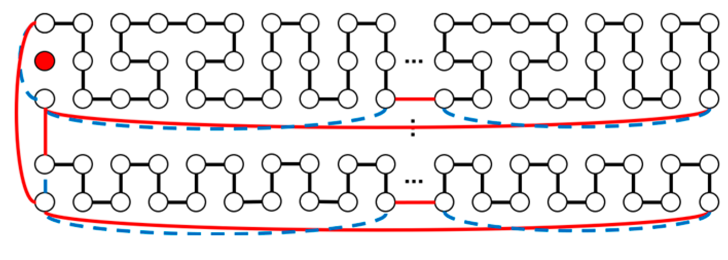
2. Main Research Results

Due to the complexity of the faulty vertex problem, this section mainly discusses it. Note that since the toroidal mesh graph is vertex-symmetric [24], the faulty vertex can be assumed to be any position in the graph. Finding a dimension-balanced Hamiltonian cycle in the graph with the faulty vertex in any position suffices. This section discusses the problem based on the parity of m and n.

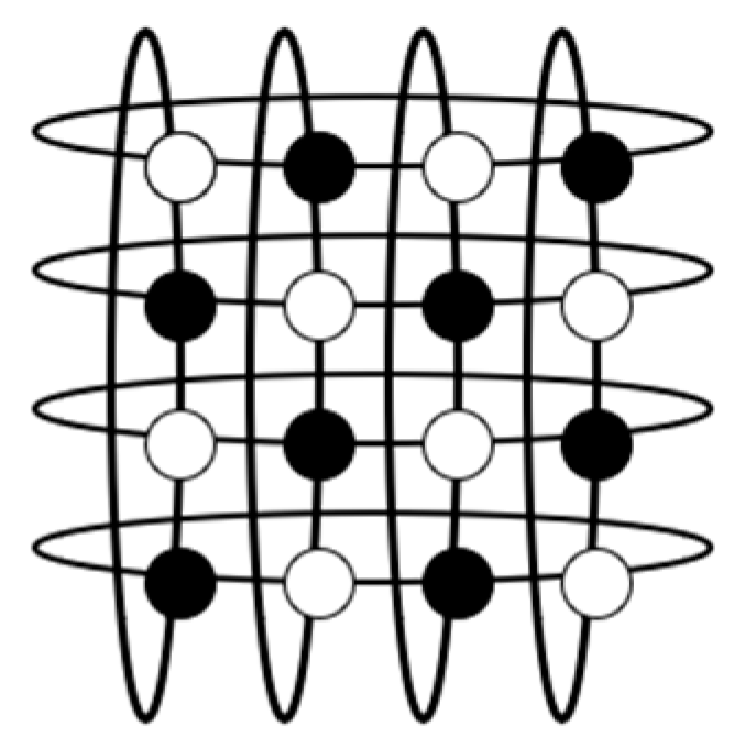
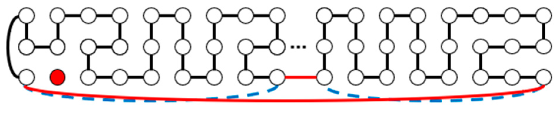
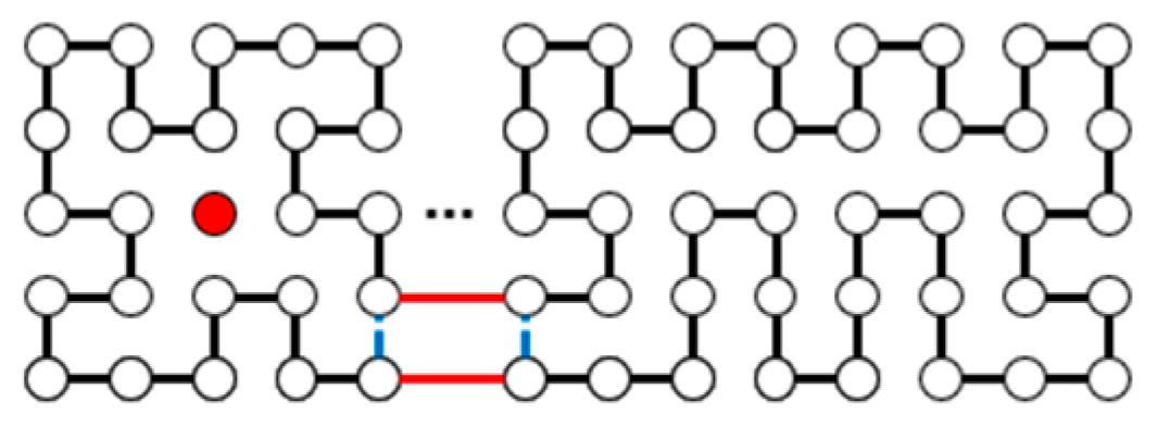
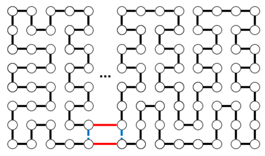
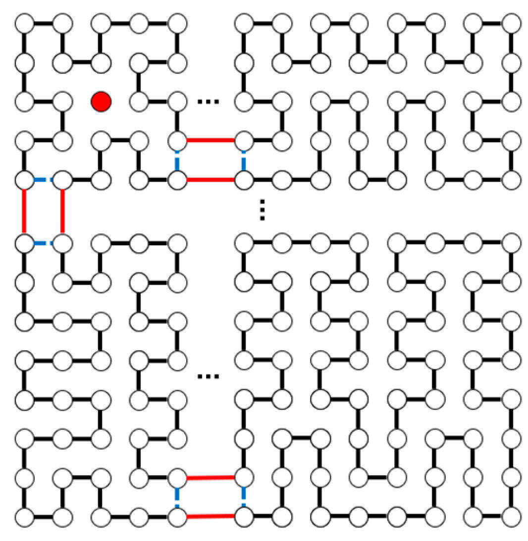
2.1. Both m and n Are Even

Theorem 1.

When both m and n are even, T_m,n − f does not have a dimension-balanced Hamiltonian cycle, where f is any vertex in the graph.

Proof of Theorem 1.

Since both m and n are even, the vertices can be divided into black and white vertices in an alternating manner (see Figure 2 as an example), ensuring black vertices are only connected to white vertices and vice versa. Thus, T_m,n can be considered a bipartite graph. The cycle in a bipartite graph must have an even number of vertices. When both m and n are even, mn − 1 is odd. Thus, T_m,n − f does not have a Hamiltonian cycle, and therefore, it does not have a dimension-balanced Hamiltonian cycle. □

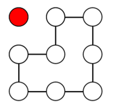
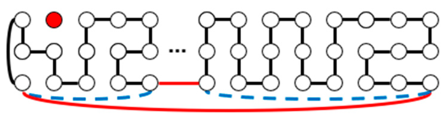
2.2. Both m and n Are Odd

This section discusses whether T_m,n − f has a dimension-balanced Hamiltonian cycle when both m and n are odd. The proof will be given through two theorems, with all cases classified based on the remainders of m and n divided by 8. A detailed classification is shown in

Table 1. Classification of cases when both m and n are odd.

	m	m, n Are Odd
n		3	5 + 8p	7 + 8p	9 + 8p	11+ 8p
3		Thm. 2 (a)	Thm. 2 (b)	Cor. 1	Thm. 2 (c)	Cor. 1
5 + 8q		Thm. 2 (b)	Thm. 3 (a)	Thm. 3 (b)	Thm. 3 (c)	Thm. 3 (d)
7 + 8q		Cor. 1	Thm. 3 (b)	Thm. 3 (e)	Thm. 3 (f)	Thm. 3 (g)
9 + 8q		Thm. 2 (c)	Thm. 3 (c)	Thm. 3 (f)	Thm. 3 (h)	Thm. 3 (i)
11 + 8q		Cor. 1	Thm. 3 (d)	Thm. 3 (g)	Thm. 3 (i)	Thm. 3 (j)

, where p and q are non-negative integers. Since T_m,n is vertex-symmetric, without loss of generality, we say n = 3 when m or n equals 3. First, we introduce a useful lemma.

Lemma 1

[18]. If m is odd, T_m,3 does not embed every 4k-DBC for k with 3 < k < ⌊3m/4⌋.

Corollary 1.

When m ≡ 3 (mod 4) and m ≥ 7, T_m,3 − f does not have a dimension-balanced Hamiltonian cycle, where f is any vertex in the graph.

Proof of Corollary 1.

Let m = 7 + 4p, where p is a non-negative integer. The number of vertices of T_{m, 3} − f is 20 + 12p = 4(5 + 3p). According to Lemma 1, we know that T_{m, 3} does not have a DBC with a length of 4(5 + 3p). So, T_{m, 3} − f does not have a DBH, where f is any vertex in the graph. □

In the following figures, the red dot represent faulty vertex f in each figure; the blue dashed lines represent edges that will be removed when forming a larger image, and the red lines represent newly added edges, for convenience.

Theorem 2.

When m = 3 or m ≡ 1 (mod 4), T_m,3 − f has a dimension-balanced Hamiltonian cycle, where f is any vertex in the graph.

Proof of Theorem 2.

The following will be divided into three cases to prove this theorem.

Case (a).

When m = 3: It can be seen from Figure 3 that T_m,3 − f has a dimension-balanced Hamiltonian cycle. In the figure, the red node denotes the faulty vertex. In the subsequent figures, the red nodes have the same meaning.

Case (b).

When m = 5 + 8p, n = 3: Figure 4 shows how to form a DBH in T_5+8p,3 − f from one DBH in T_5,3 − f and p DBHs in T_8,3. In this case, if we delete the edge set {(0, 2)(4, 2)} ∪ {(5 + 8x, 2)(12 + 8x, 2) | 0 ≤ x < p} and add {(0, 2)(4 + 8p, 2)} ∪ {(4 + 8x, 2)(5 + 8x, 2) | 0 ≤ x < p}, we obtain the Hamiltonian cycle C onT_5+8p,3 − f, where |E₁(C)| = 7 + 12p = |E₂(C)|. Therefore, ||E₁(C)| − |E₂(C)|| = 0, and cycle C satisfies the condition of dimension balance, so C is a DBH on T_5+8p,3 − f. In Figure 4, the blue dotted lines represent the edges that need to be deleted when merging the graphs, and the red lines represent the edges that need to be added when merging the graphs. In the subsequent figures, the blue dotted lines and the red lines have the same meaning.

Case (c).

When m = 9 + 8p, n = 3: Figure 5 shows how to form a DBH in T_9+8p,3 − f from one DBH in T_9,3 − f and p DBHs in T_8,3. In this case, if we delete the edge set {(0, 2)(8, 2)} ∪ {(9 + 8x, 2)(16 + 8x, 2) |0 ≤ x < p} and add {(0, 2)(8 + 8p, 2)} ∪ {(8 + 8x, 2), (9 + 8x, 2) |0 ≤ x < p}, we obtain the Hamiltonian cycle C on T_9+8p,3 − f, where |E₁(C)| = 13 + 12p = |E₂(C)|. Therefore, ||E₁(C)| − |E₂(C)|| = 0, and cycle C satisfies the condition of dimension balance, so C is a DBH on T_9+8p,3 − f. □

Theorem 3.

When m and n are both odd integers greater than 4, T_m,n − f has a dimension-balanced Hamiltonian cycle, where f is any vertex in the graph.

Proof of Theorem 3.

The following will be divided into ten cases for discussion based on the remainder of m and n divided by eight.

Case (a).

When m = 5 + 8p, n = 5 + 8q: Firstly, as Figure 6 shows, if we put p HCs (Hamiltonian cycles) of T_8,5 on the right hand side of the DBH of T_5,5 − f, delete the edge set {(4 + 8x, 3)(4 + 8x, 4) | 0 ≤ x < p} ∪ {(5 + 8x, 3)(5 + 8x, 4) | 0 ≤ x < p}, and add {(4 + 8x, 3)(5 + 8x, 3) | 0 ≤ x < p} ∪ {(4 + 8x, 4)(5 + 8x, 4) | 0 ≤ x < p}, we obtain a DBH C₁ of T_5+8p,5 − f, where |E₁(C₁)| = 12 + 20p = |E₂(C₁)|. On the other hand, as Figure 7 shows, if we put p HCs of T_8,8 on the right hand side of the HC of T_5,8, delete the edge set {(4 + 8x, 6)(4 + 8x, 7) | 0 ≤ x < p} ∪ {(5 + 8x, 6)(5 + 8x, 7) | 0 ≤ x < p}, and add {(4 + 8x, 6)(5 + 8x, 6) | 0 ≤ x < p} ∪ {(4 + 8x, 7)(5 + 8x, 7) | 0 ≤ x < p}, an HC C₂ of T_5+8p,8 is obtained, where|E₁(C₂)| = 22 + 32p, and |E₂(C₂)| = 18 + 32p. Lastly, if we put q C₂s under C₁ then delete the edge set {(0, 4 + 8x)(1, 4 + 8x) | 0 ≤ x < q } ∪ {(0, 5 + 8x)(1, 5 + 8x) | 0 ≤ x < q} and add the edge set {(0, 4 + 8x)(0, 5 + 8x) | 0 ≤ x < q} ∪ {(1, 4 + 8x)(1, 5 + 8x) | 0 ≤ x < q}, there is an HC C₃ of T_5+8p,5+8q − f (see Figure 8 for an illustration), where |E₁(C₃)| = 12 + 20p + q(20 + 32p) = |E₂(C₃)|; therefore, C₃ is a DBH of T_5+8p,5+8q − f. In Figure 8 and the subsequent figures, similarly to the previous theorem, the red node denotes the faulty vertex, the blue dotted lines represent the edges that need to be deleted when merging the graphs, and the red lines represent the edges that need to be added when merging the graphs.

Case (b).

When m = 7 + 8p, n = 5 + 8q: In this case, similarly to case (a), a DBH for T_7+8p,5+8q − f will be constructed. Please refer to Figure 9 for the DBH of T_7,5 − f, DBH of T_8,5, DBH of T_7,8, HC of T_8,8 and construction method. The obtained HC C on T_7+8p,5+8q − f has |E₁(C)| = 17 + 20p + q(28 + 32p) = |E₂(C)|, so C is a DBH on T_7+8p,5+8q − f. Since T_m,n has symmetry, by transposing this figure, a DBH on T_5+8p,7+8q − f can be obtained. Every subsequent case when m and n are not equal has this property, which will not be described again.

Case (c).

When m = 9 + 8p, n = 5 + 8q: Similarly to case (a), a DBH for T_9+8p,5+8q − f will be constructed with a DBH of T_9,5 − f, p HCs of T_8,5, q HCs of T_9,8, and pq HCs of T_8,8. Please refer to Figure 10. The constructed HC C has |E₁(C)| = 22 + 20p + q(36 + 32p) = |E₂(C)|. Therefore, C is a DBH of T_9+8p,5+8q − f.

Case (d).

When m = 11 + 8p, n = 5 + 8q: Similarly to case (b), a DBH for T_11+8p,5+8q − f will be constructed with a DBH of T_11,5 − f, p DBHs of T_8,5, q DBHs of T_11,8, and pq HCs of T_8,8. Please refer to Figure 11. The constructed HC C has |E₁(C)| = 27 + 20p + q(44 + 32p) = |E₂(C)|. Therefore, C is a DBH of T_11+8p,5+8q − f.

Case (e).

When m = 7 + 8p, n = 7 + 8q: Similarly to case (a), a DBH for T_7+8p,7+8q − f will be constructed with a DBH of T_7,7 − f, p HCs of T_8,7, q HCs of T_7,8, and pq HCs of T_8,8. Please refer to Figure 12. The constructed HC C has |E₁(C)| = 24 + 28p + q(28 + 32p) = |E₂(C)|. Therefore, C is a DBH of T_7+8p,7+8q − f.

Case (f).

When m = 9 + 8p, n = 7 + 8q: Similarly to case (b), a DBH for T_9+8p,7+8q − f will be constructed with a DBH of T_9,7 − f, p HCs of T_8,7, q DBHs of T_9,8, and pq HCs of T_8,8. Please refer to Figure 13. The constructed HC C has |E₁(C)| = 31 + 28p + q(36 + 32p) = |E₂(C)|. Therefore, C is a DBH of T_9+8p,7+8q − f.

Case (g).

When m = 11 + 8p, n = 7 + 8q: Similarly to case (a), a DBH for T_11+8p,7+8q − f will be constructed with a DBH of T_11,7 − f, p HCs of T_8,7, q HCs of T_11,8, and pq HCs of T_8,8. Please refer to Figure 14. The constructed HC C has |E₁(C)| = 38 + 28p + q(44 + 32p) = |E₂(C)|. Therefore, C is a DBH of T_11+8p,7+8q − f.

Case (h).

When m = 9 + 8p, n = 9 + 8q: Similarly to case (a), a DBH for T_9+8p,9+8q − f will be constructed with a DBH of T_9,9 − f, p HCs of T_8,9, q HCs of T_9,8, and pq HCs of T_8,8. Please refer to Figure 15. The constructed HC C has |E₁(C)| = 40 + 36p + q(36 + 32p) = |E₂(C)|. Therefore, C is a DBH of T_9+8p,9+8q − f.

Case (i).

When m = 11 + 8p, n = 9 + 8q: Similarly to case (b), a DBH for T_11+8p,9+8q − f will be constructed with a DBH of T_11,9 − f, p DBHs of T_8,9, q HCs of T_11,8, and pq HCs of T_8,8. Please refer to Figure 16. The constructed HC C has |E₁(C)| = 49 + 36p + q(44 + 32p) = |E₂(C)|. Therefore, C is a DBH of T_11+8p,9+8q − f.

Case (j).

When m = 11 + 8p, n = 11 + 8q: Similarly to case (a), a DBH for T_11+8p,11+8q − f will be constructed with a DBH of T_11,11 − f, p HCs of T_8,11, q HCs of T_11,8, and pq HCs of T_8,8. Please refer to Figure 17. The constructed HC C has |E₁(C)| = 60 + 44p + q(44 + 32p) = |E₂(C)|. Therefore, C is a DBH of T_11+8p,11+8q − f.

From the analysis of the above ten cases, it can be seen that when m and n are both odd numbers, even if there is a faulty vertex f, a DBH can be created in T_m,n − f, so the proof is completed. □

2.3. One of m and n Is Even and the Other Is Odd

This section will discuss whether T_m,n − f still has a dimension-balanced Hamiltonian cycle when one of m and n is even and the other is odd. The following theorem is the main analytical result of this section, which discusses all possibilities of the remainder after dividing m by 8. Please refer to

Table 2. Classification of cases when one of m and n is even and the other is odd.

	m	m Is Even and n Is Odd
n		4 + 8p	6 + 8p	8 + 8p	10 + 8p
3 + 2q		Thm. 4 (a)	Thm. 4 (b)	Thm. 4 (c)	Thm. 4 (d)

for specific classification cases, where p and q are non-negative integers. Since T_m,n is equivalent to C_m × C_n and isomorphic to C_n × C_m, it can be assumed without loss of generality that m is an even number and n is an odd number. When n is an even number and m is an odd number, the corresponding DBH can be obtained by transposing the DBH obtained in the theorem (horizontally versus vertically).

For convenience, Y_m is defined as the graph generated by the Cartesian product of C_m and P₂, which is called a prism graph, where P_n is the path of n vertices. Compared to T_m,n, the vertex set is the same and the edge set is the edge that lacks “crossing” edges in the vertical part (in fact, the vertical part only has two vertices, and the original definition is that there is an edge connecting the two vertices). It is defined as follows: vertex set V(Y_m) = {(x, y) | 0 ≤ x ≤ m − 1; 0 ≤ y ≤ 1}; edge set E(Y_m) = {(x₁, y₁)(x₂, y₂) | x₁ = x₂ and |y₁ − y₂| = 1, or |x₁ − x₂| = (1 or m − 1) and y₁ = y₂}. On the other hand, $Y_n^T$ represents the graph generated by the Cartesian product of P₂ and C_m, and its vertex set V($Y_n^T$) = {(x, y) | 0 ≤ x ≤ 1; 0 ≤ y ≤ m − 1}, and its edge set E($Y_n^T$) = {(x₁, y₁)(x₂, y₂) | x₁ = x₂ and |y₁ − y₂| = (1 or n − 1), or |x₁ − x₂| = 1 and y₁ = y₂}.

Theorem 4.

When one of m and n is even and the other is odd integer, both are greater than 2, T_m, n − f has a dimension-balanced Hamiltonian cycle, where f is any vertex in the graph.

Proof of Theorem 4.

Without loss of generality, it is assumed that m is an even number and n is an odd number. Since m, n ≥ 3, we start from the graph of T_4,3 to find the dimension-balanced Hamiltonian cycle when there is a faulty vertex. As shown in Table 2, four cases are discussed based on the remainder of m divided by eight.

Case (a).

m = 4 + 8p, n = 3 + 2q: Firstly, please refer to Figure 18. If we put p DBHs of T_8,3 on the right hand side of the DBH of T_4,3 − f, delete the edge set {(0, 2)(3, 2)} ∪ {(4 + 8x, 2)(11 + 8x, 2) | 0 ≤ x < p}, and add {(0, 2)(3 + 8p, 2)} ∪ {(3 + 8x, 2)(4 + 8x, 2) | 0 ≤ x < p}, we obtain a DBH C₁ of T_4+8p,3 – f, where |E₁(C₁)| = 6 + 12p, |E₂(C₁)| = 5 + 12p. Again, in Figure 18 and the subsequent figures, the red node denotes the faulty vertex, the blue dotted lines represent the edges that need to be deleted when merging the graphs, and the red lines represent the edges that need to be added when merging the graphs.

Next, as Figure 19 shows, if we put p DBHs of Y₈ on the right hand side of the DBH of Y₄, delete the edge set {(0, 4)(3, 4)} ∪ {(4 + 8x, 4)(11 + 8x, 4) | 0 ≤ x < p}, and add {(0, 4)(3 + 8p, 4)} ∪ {(3 + 8x, 4), (4 + 8x, 4) | 0 ≤ x < p}, a DBH C₂ of Y_4+8p is obtained, where |E₁(C₂)| = 4 + 8p = |E₂(C₂)|.

Lastly, if we put q C₂s under C₁ then delete the edge set {(0, 0)(0, 2)} ∪ {(0, 3 + 2x)(0, 4 + 2x) | 0 ≤ x < q} and add the edge set {(0, 0)(0, 2 + 2q)} ∪ {(0, 2 + 2x), (0, 3 + 2x) | 0 ≤ x < q}, there is an HC C₃ of T_4+8p,3+2q − f. As Figure 20 shows, after the calculation, |E₁(C₃)| = 6 + 12p + q(4 + 8p), |E₂(C₃)| = 5 + 12p + q(4 + 8p); therefore, C₃ is a DBH of T_4+8p,3+2q − f because ||E₁(C₃)| − |E₂(C₃)|| = 1.

Case (b).

m = 6 + 8p, n = 3 + 2q: Similarly to case (a), a DBH for T_6+8p,3+2q − f will be constructed with a DBH of T_6,3 − f, the same p DBHs of T_8,3, q DBHs of Y₆, and the same pq DBHs of Y₈. Please refer to Figure 21. Place p DBHs of T_8,3 on the right side of the DBH of T_6,3 − f. After deleting and connecting the appropriate edges, the DBH C₁ at T_6+8p,3 is obtained. Then, place p DBHs of Y₈ to the right of the DBH of Y₆, and after deleting and connecting the appropriate edges, the DBH C₂ at T_6+8p,8 can be obtained. Finally, place q pieces of C₂s under C₁, delete and connect the appropriate edges, and obtain the HC C₃ at T_6+8p,3+2q. Since |E₁(C₃)| = 8 + 12p + q(6 + 8p), |E₂(C₃)| = 9 + 12p + q(6 + 8p). Therefore ||E₁(C₃)| − |E₂(C₃)|| = 1, C₃ is a DBH on T_6+8p,3+2q − f.

Case (c).

m = 8 + 8p, n = 3 + 2q: Similarly to case (a), a DBH for T_8+8p,3+2q − f will be constructed with a DBH of T_8,3 − f, the same p DBHs of T_8,3, and the same q + pq DBHs of Y₈. Please refer to Figure 22, which shows how to connect these DBHs to form an HC C of T_8+8p,3+2q. Since |E₁(C)| = 12 + 12p + q(8 + 8p), |E₂(C)| = 11 + 12p + q(8 + 8p). Therefore ||E₁(C)| − |E₂(C)|| = 1, C is a DBH on T_8+8p,3+2q − f.

Case (d).

m = 10 + 8p, n = 3 + 2q: Similarly to case (a), a DBH for T_10+8p,3+2q − f will be constructed with a DBH of T_10,3 − f, the same p DBHs of T_8,3, q DBHs of Y₁₀, and the same pq DBHs of Y₈. Please refer to Figure 23, which shows how to connect these DBHs to form an HC C of T_10+8p,3+2q. Since |E₁(C)| = 14 + 12p + q(10 + 8p), |E₂(C)| = 15 + 12p + q(10 + 8p). Therefore ||E₁(C)| − |E₂(C)|| = 1, C is a DBH on T_10+8p,3+2q − f.

From the analysis of the above four cases, it can be known that for all m and n that are an even number and an odd number, respectively, if there is a faulty vertex, a DBH in T_m,n − f can be obtained. Therefore, this proof is completed. □

3. Conclusions

From the discussion in the previous section, it can be seen that in most cases of m and n, the dimension-balanced Hamiltonian cycle DBH can be found in T_m,n − f for any faulty vertex f. The following corollary can be drawn.

Corollary 2.

Assuming that f is any vertex in the graph T_m,n, T_m,n − f has a dimension-balanced Hamiltonian cycle DBH, except in the following cases:

(1) When m and n are both even numbers;

(2) When one of m and n is 3, and the other satisfies mod 4 = 3 and is greater than 6.

Proof of Corollary 2.

According to Theorem 1 and Corollary 1, we know there is no dimension-balanced Hamiltonian cycle on T_m,n − f for any faulty vertex f when (1) both m and n are even or (2) one of m and n is 3 and the other satisfies mod 4 = 3 and is greater than 6. On the other hand, according to Theorems 2–4, T_m,n − f has a dimension-balanced Hamiltonian cycle DBH when the above is not true for m and n. □

In addition, there are three conjectures in the literature [18]. If the following conjecture (that is, Conjecture 1) is true, the other two conjectures (that is, Conjectures 2 and 3) are also true, since it has already been proven in the remaining cases.

Conjecture 1

[18]. When m and n ≥ 5 are both odd numbers, for k = ⌊(mn − 1)/4⌋, there is a DBC of length 4k in T_m,n.

Conjecture 2

[18]. For odd m and n ≥ 5, T_m,n is (2max{m, n} − 1)-DBP.

Conjecture 3

[18]. For odd m and n ≥ 5, T_m,n is (2max{m, n} − 1)-DBVP.

Since it has been proven in [18] that when k = ⌊(mn − 3)/4⌋, there is a DBC of length 4k in T_m,n, we only need to discuss when k = (mn − 1)/4, that is, when mn − 1 = 4k. Theorem 3 (a), (c), (e), (g), (h), and (j) answer this question, so this paper also proves the correctness of the three conjectures in the literature [18]. And the following corollary can be concluded.

Corollary 3.

When m and n ≥ 5 are both odd numbers, for k = ⌊ (mn − 1) / 4 ⌋, there is a DBC of length 4k in T_m,n; therefore T_m,n is (2max { m, n } − 1)-DBP and (2max { m, n } − 1)-DBVP.

In addition, the following has been proven in [16]:

Theorem 5 [16].

There are dimension-balanced Hamiltonian cycles for T_m,n, except mn ≡ 2 (mod 4), that is, one of m and n is odd and the other satisfies mod 4 = 2.

Since a Hamiltonian cycle does not use all of its edges (in fact, there are two edges at any vertex that are not used), and because T _m,n is a vertex-symmetric graph, if any edge is faulty, then through appropriate rotation, a dimension-balanced Hamilton cycle without using the faulty edge can be obtained. That is to say, the following corollary can be drawn.

Corollary 4.

There are dimension-balanced Hamiltonian cycles for T_m,n – e, except mn ≡ 2 (mod 4), where e is any edge of T_m,n.

According to Corollaries 2 and 4 and the definition of one-fault dimension-balanced Hamiltonian, we draw the following conclusion.

Corollary 5.

T_m,n is one-fault dimension-balanced Hamiltonian, except in the following cases:

(1) When m and n are both even numbers;

(2) When one of m and n is 3, and the other satisfies mod 4 = 3 and is greater than 6;

(3) When one of m and n is odd, and the other satisfies mod 4 = 2.

Proof of Corollary 5.

Corollary 2 shows that T_m,n − f has a DBH for any node f, except (1) or (2). So, T_m,n is not one-fault dimension-balanced Hamiltonian when (1) or (2) holds. Corollary 4 shows that T_m,n − e has a DBH for any edge e, except (3). So, T_m,n is not one-fault dimension-balanced Hamiltonian when (3) holds. In addition, since it is true that T_m,n − f and T_m,n − e both have a DBH, except (1), (2), and (3), T_m,n is one-fault dimension-balanced Hamiltonian, except (1), (2), and (3). □

Table 3. A brief summary of previously obtained results and our results.

Reference	Multiprocessor Systems	Problems
[5]	Toroidal mesh graph (Tm,n)	two-fault H
[16]	Toroidal mesh graph (Tm,n)	DBH
[18]	Toroidal mesh graph (Tm,n)	DBP
[19]	Toroidal mesh graph (Tm,n)	WDBH
[20]	Toroidal mesh graph (Tm,n)	WDBP
[21]	3-dimensional toroidal mesh graph (Tm,n,r)	DBH
This paper	Toroidal mesh graph (Tm,n)	one-fault DBH and DBP

shows a comparison of this study with previous works. Where two-fault H means two-fault Hamiltonian. Note that the DBP and WDBH problem under other conditions (both m and n are even, or one of them is even and the other is odd) has also been studied already. The DBP and WDBP problem is completed by [18] and [20], respectively (except for the DBP problem, three conjectures remain unsolved). From Table 3, it can be observed that, compared to previous works, our study is the first to investigate the one-fault DBH problem on T_m,n. Moreover, we resolved a conjecture previously left open in the DBP problem on T_m,n, thereby completing the solution of the DBP problem.

It is not difficult to see, based on Theorems 2–5, that an algorithm for identifying a dimension-balanced Hamiltonian cycle on a toroidal mesh network (T_m,n) can be obtained when given the input size m, n and the locations of faulty nodes. Since the automorphism adjustment based on the faulty node or edge is performed in linear time, the time complexity of the algorithm is proportional to the length of the Hamiltonian cycle, which is O (mn).

In 2000, [5] proved that if m ≥ 3, n ≥ 3, and n is odd, T_m,n − F has a Hamiltonian cycle for any F with |F| ≤ 2. And whether T_m,n − F has a DBH for any F with |F| = 1 has been solved in this paper. Therefore, building on the current results, a potential future research direction is to explore the conditions under which a toroidal mesh graph T_m,n in this partition is two-fault dimension-balanced Hamiltonian based on the values of m and n. Additionally, another avenue for future study could involve investigating the dimension-balanced Hamiltonian cycle problem on a toroidal mesh graph under different partitioning schemes, expanding the applicability of the proposed approach. Please note that the DBHs constructed in this paper are all discussed based on the edge partitions E₁ and E₂ defined at the beginning of this paper, and there is no guarantee that there is a DBH on T_m,n − f or T_m,n – e for any partition of the edge set. Therefore, such studies could provide deeper insights into the fault tolerance and adaptability of Hamiltonian cycles in various configurations of toroidal mesh graphs.

References

1. Cada, R.; Flandrin, E.; Li, H. Hamiltonicity and pancyclicity of cartesian products of graphs. Discret. Math. 2009, 309, 6337–6343. [Google Scholar] [CrossRef]
2. Kühn, D.; Osthus, D. A survey on Hamilton cycles in directed graphs. Eur. J. Comb. 2012, 33, 750–766. [Google Scholar] [CrossRef]
3. Li, R. A degree sum condition for Hamiltonian graphs. Electron. J. Math. 2021, 1, 85–88. [Google Scholar]
4. Yang, Y. Hyper-Hamiltonian Laceability of Cartesian Products of Cycles and Paths. Comput. J. 2024, 67, 548–556. [Google Scholar] [CrossRef]
5. Kim, H.-C.; Park, J.-H. Fault Hamiltonicity of Two-Dimensional Torus Networks. In Proceedings of the Workshop on Algorithms and Computation WAAC’00, Tokyo, Japan, 21–22 July 2000; pp. 110–117. [Google Scholar]
6. Goddard, W.; Henning, M.A. Note Pancyclicity of the prism. Discret. Math. 2001, 234, 139–142. [Google Scholar] [CrossRef]
7. Hsu, H.-C.; Chiang, L.-C.; Tan, J.J.; Hsu, L.-H. Fault hamiltonicity of augmented cubes. Parallel Comput. 2005, 31, 131–145. [Google Scholar] [CrossRef]
8. Dimakopoulos, V.V.; Palios, L.; Poulakidas, A.S. On the hamiltonicity of the cartesian product. Inform. Process. Lett. 2005, 96, 49–53. [Google Scholar] [CrossRef]
9. Yang, M.C.; Tan, J.J.; Hsu, L.H. Hamiltonian circuit and linear array embeddings in faulty k-ary n-cubes. J. Parallel Distrib. Comput. 2007, 67, 362–368. [Google Scholar] [CrossRef]
10. Hsieh, S.-Y.; Wu, C.-Y. Edge-fault-tolerant hamiltonicity of locally twisted cubes under conditional edge faults. J. Comb. Optim. 2010, 19, 16–30. [Google Scholar] [CrossRef]
11. Cheng, C.-W.; Lee, C.-W.; Hsieh, S.-Y. Conditional edge-fault hamiltonicity of cartesian product graphs. IEEE Trans. Parallel Distrib. Syst. 2012, 24, 1951–1960. [Google Scholar] [CrossRef]
12. Hsieh, S.-Y.; Cian, Y.-R. Conditional edge-fault hamiltonicity of augmented cubes. Inform. Sci. 2010, 180, 2596–2617. [Google Scholar] [CrossRef]
13. Du, Z.-Z.; Xu, J.-M. A note on cycle embedding in hypercubes with faulty vertices. Inf. Process. Lett. 2011, 111, 557–560. [Google Scholar] [CrossRef]
14. Wang, Y.-C.; Juan, J.S.-T. Hamiltonicity of the Basic WK-recursive Pyramid with and without Faulty Nodes. Theor. Comput. Sci. 2015, 561, 542–556. [Google Scholar] [CrossRef]
15. Abdallah, M.; Cheng, E. Fault-tolerant Hamiltonian connectivity of 2-tree-generated networks. Theor. Comput. 2022, 907, 62–81. [Google Scholar] [CrossRef]
16. Peng, W.-F.; Juan, J.S.-T. The balanced Hamiltonian cycle on the Toroidal mesh graphs. In Proceedings of the World Academy of Science, Engineering and Technology, Tokyo, Japan, 29–30 May 2012; Volume 65, pp. 1047–1053. [Google Scholar]
17. Zheng, S.Y.; Hu, H.L.; Xu, X.; Le, K. Structured-light-based 3D reconstruction using Gray code and line-shift stripes. Adv. Mater. Res. 2010, 108, 799–804. [Google Scholar] [CrossRef]
18. Juan, J.S.-T.; Peng, W.-F.; Lai, Z.-Y. The dimension-balanced pancyclicity on Tm,n for both m and n are odd. In Proceedings of the International Conference on Parallel and Distributed Processing Techniques and Applications (PDPTA’21), Luxor, Las Vegas, NA, USA, 26–29 July 2021. [Google Scholar]
19. Wu, R.-Y.; Lai, Z.-Y.; Juan, J.S.-T. The weakly dimension-balanced Hamiltonian. In Proceedings of the International Conference on Parallel and Distributed Processing Techniques and Applications (PDPTA’18), Luxor, Las Vegas, NA, USA, 30 July–2 August 2018; pp. 178–182. [Google Scholar]
20. Juan, J.S.-T.; Lai, Z.-Y. The weakly dimension-balanced pancyclicity on Toroidal mesh graph Tm,n when both m and n are odd. In Computing and Combinatorics. COCOON 2021. Lecture Notes in Computer Science; Chen, C.Y., Hon, W.K., Hung, L.J., Lee, C.W., Eds.; Springer International Publishing: Berlin/Heidelberg, Germany, 2021; Volume 13025, pp. 437–448. [Google Scholar]
21. Juan, J.S.-T.; Tseng, Y.-H.; Lai, C.-S.; Lai, Z.-Y. Dimension-balanced Hamiltonian cycle on 3-dimensional Toroidal mesh graph. In Proceedings of the International Congress on Engineering and Information (ICEAI’19), Osaka, Japan, 7–9 May 2019; pp. 47–57. [Google Scholar]
22. Tedesco, L.; Mello, A.; Garibotti, D.; Calazans, N.; Moraes, F. Traffic Generation and Performance Evaluation for Mesh-based NoCs. In Proceedings of the 18th Annual Symposium on Integrated Circuits and System Design (SBCCI’05), Florianolpolis, Brazil, 4–7 September 2005; Association for Computing Machinery: New York, NY, USA, 2005; pp. 184–189. [Google Scholar]
23. Nain, Z.; Ali, R.; Anjum, S.; Afzal, M.K.; Kim, S.W. A network adaptive fault-tolerant routing algorithm for demanding latency and throughput applications of network-on-a-chip designs. Electronics 2020, 9, 1076. [Google Scholar] [CrossRef]
24. Xu, J. Theory and Application of Graphs; Springer Science & Business Media: Berlin/Heidelberg, Germany, 2013. [Google Scholar]
Figure 1. T4,3.
Symmetry 17 00093 g001
Figure 2. Viewing Tm,n as a bipartite graph.
Symmetry 17 00093 g002
Figure 3. There is a DBH in T3,3f.
Symmetry 17 00093 g003
Figure 4. There is a DBH in T5+8p,3f.
Symmetry 17 00093 g004
Figure 5. There is a DBH in T9+8p,3f.
Symmetry 17 00093 g005
Figure 6. The DBH C1 of T5+8p,5f.
Symmetry 17 00093 g006
Figure 7. The HC C2 of T5+8p,8.
Symmetry 17 00093 g007
Figure 8. The DBH C3 of T5+8p,5+8qf.
Symmetry 17 00093 g008
Figure 9. The DBH of T7+8p,5+8qf.
Symmetry 17 00093 g009
Figure 10. The DBH of T9+8p,5+8qf.
Symmetry 17 00093 g010
Figure 11. The DBH of T11+8p,5+8qf.
Symmetry 17 00093 g011
Figure 12. The DBH of T7+8p,7+8qf.
Symmetry 17 00093 g012
Figure 13. The DBH of T9+8p,7+8qf.
Symmetry 17 00093 g013
Figure 14. The DBH of T11+8p,7+8qf.
Symmetry 17 00093 g014
Figure 15. The DBH of T9+8p,9+8qf.
Symmetry 17 00093 g015
Figure 16. The DBH of T11+8p,9+8qf.
Symmetry 17 00093 g016
Figure 17. The DBH of T11+8p,11+8qf.
Symmetry 17 00093 g017
Figure 18. The DBH of T4+8p,3f.
Symmetry 17 00093 g018
Figure 19. The DBH of Y4+8pf.
Symmetry 17 00093 g019
Figure 20. The DBH of T4+8p,3+2qf.
Symmetry 17 00093 g020
Figure 21. The DBH of T6+8p,3+2qf.
Symmetry 17 00093 g021
Figure 22. The DBH of T8+8p,3+2qf.
Symmetry 17 00093 g022
Figure 23. The DBH of T10+8p,3+2qf.
Symmetry 17 00093 g023