Abstract
With the rapid expansion of urban subway networks, vibrations induced by subway operations have become an increasingly significant concern for nearby structures. To assess the influence of subway-induced vibrations on nearby structures, it is essential to predict the vibration effects accurately prior to the construction of the subway system. By combining an improved Long Short-Term Memory (LSTM) model with a spectral analysis, this paper proposes a hybrid method to enhance the accuracy and efficiency of predicting structural vibrations induced by subway operations. The improved LSTM model is composed of BiLSTM, an attention mechanism, and the DBO algorithm. The symmetry inherent in the vibration propagation paths and the structural layouts of subway systems is leveraged to improve the feature extraction and modeling accuracy. Additionally, the hybrid method utilizes the symmetric properties of vibration signals in the spectral domain to enhance prediction robustness and efficiency. Then, the hybrid method is utilized to rapidly achieve highly accurate vibration responses induced by subway operations. The verification results demonstrate the following: (1) The improved LSTM model enhances the ability to recognize patterns in time-series vibration data, leading to improved model convergence and generalization. The improved LSTM mode has a significant improvement in prediction accuracy compared to the standard LSTM network. For numerical simulation and real-world measured signals, values of R2 increased by 3% and 49.37%. (2) The proposed hybrid method significantly reduces computational time while ensuring results consistent with those obtained from the time-history analysis method. Applying the proposed hybrid method for data augmentation enhances the accuracy of the spectral analysis. The hybrid method achieves an improvement of 7% for the prediction accuracy.
1. Introduction
Subway systems, serving as the backbone of urban transportation, generate vibrations that influence the surrounding environment, including buildings, roads, and other infrastructure. These impacts are predominantly observed in three key areas: (1) construction activities may cause varying levels of damage to existing structures; (2) vibrations from subway operations can disrupt the daily lives of residents; and (3) sensitive instruments may experience data distortion or even operational malfunctions due to subway-induced vibrations [1].
Accurately predicting subway-induced vibrations is essential for mitigating their impact, particularly in densely populated urban areas. Various approaches have been proposed for this purpose, including empirical prediction methods, numerical simulation techniques, and experimental prediction methods. Empirical prediction methods use field data or established empirical equations to estimate the vibration responses caused by subway operations. Due to their simplicity and computational efficiency, these methods are typically utilized for preliminary assessments. Parameters such as train speed, track conditions, soil types, and distance from the subway line are often employed in these methods to estimate vibration levels. The earliest works in this field were conducted by Kurzweil [2], Melke [3], and Madshus and Kaynia [4], who developed the earliest empirical equations for predicting vibrations in layered soils. These empirical equations considered parameters such as soil stiffness and train speed. Although effective under specific conditions, they often lack generalizability across diverse site conditions. Based on a series of ground vibration measurements at different sites, Bahrekazemi [5] presented two different semiempirical models for the prediction of ground-borne vibration due to train traffic. Tao et al. [6] focuses on predicting train-induced floor vibrations and structure-borne noise in low-rise buildings constructed above railway tracks. They developed a detailed computational model that accounts for train dynamics, track-structure interactions, and the vibration transmission through the building’s foundation and floors. Kedia et al. [7] developed empirical relations to predict ground vibrations caused by underground metro trains. By analyzing various factors such as train speed, track conditions, and soil properties, the study establishes mathematical models that can estimate vibration levels at different distances from the track. Despite these advancements, empirical prediction methods remain limited, as they cannot account for all environmental variables and have restricted applicability in regions with varying geological conditions. Numerical simulation methods have become an indispensable tool in predicting subway-induced vibrations due to the ability to model complex interactions between the subway system, soil layers, and surrounding structures. Structural elements such as subway tunnels, track systems, and surrounding environments often exhibit symmetrical or repetitive geometrical and material properties, which play a crucial role in the propagation of vibration waves. The Finite Element Method (FEM) and Boundary Element Method (BEM) are two of the most widely used approaches for simulating subway-induced vibrations. FEM provides detailed insight into the dynamic behavior of soil–structure systems, making it ideal for vibration prediction in urban areas with diverse ground conditions. Gupta et al. [8], Amado-Mendes et al. [9], Bian et al. [10] utilized FEM to simulate the interaction between subway trains and ground vibrations, considering the influence of train speed, track design, and soil properties. While numerical simulation methods, particularly FEM, offer detailed predictions of subway-induced vibrations, they come with a few challenges. Based on vehicle-track coupled dynamics theory, wavenumber finite element theory (2.5D FEM) and Green’s function method, Qu et al. [11] proposed a method that could comprehensively analyze vibration characteristics of the source, propagation path and sensitive target/vibration receiver by appropriately considering the boundary conditions between each part. Wu et al. [12] applied a hybrid random-vibration method combining the Finite Element Method (FEM), Boundary Element Method (BEM), and Propagation Element Method (PEM) to predict low-frequency structure-borne noise in U-shaped girders of urban rail transit systems. The approach integrated these methods to model the complex interactions between train vibrations, the structure, and the surrounding environment. Alves Costa et al. [13] investigated track–ground vibrations induced by railway traffic, focusing on in situ measurements and the validation of a 2.5D FEM-BEM model. They combined the Finite Element Method (FEM) and Boundary Element Method (BEM) to simulate the interaction between the track, ground, and vibrations caused by train movement. Despite these advancements, numerical simulations remain computationally expensive and time-consuming, especially when dealing with large-scale urban systems. Experimental prediction methods involve collecting real-world vibration data through field measurements using accelerometers, geophones, or other sensors. These methods offer a direct and practical approach to predicting subway-induced vibrations by analyzing the vibrations in actual operating conditions. Liu et al. [14] proposed a framework that combines experimental data with numerical modeling to characterize the dynamic interaction between train-induced vibrations and the surrounding ground. They evaluated the excitation forces generated by train movement and analyzed their propagation through the soil, providing insights into vibration attenuation and its dependence on factors like train speed, track design, and ground properties. He et al. [15] presented an efficient prediction model for vibrations induced by underground railway traffic, supported by experimental validation. The model integrated a simplified numerical approach with key parameters of the railway system, ground, and tunnel structure to predict vibration levels accurately and efficiently. A. Colaço et al. [16] combined experimental measurements and numerical modeling to predict ground-borne vibrations induced by railway traffic. They utilized field measurements to capture key vibration characteristics and integrated them into numerical models that simulate the propagation of vibrations through the soil and structures. Recent advancements in experimental methods include the use of different instruments for high-resolution vibration measurements [17,18,19]. In addition to field studies, laboratory experiments are increasingly used to simulate subway-induced vibrations under controlled conditions [20]. Despite the strengths of experimental methods, experimental prediction methods are resource-intensive, requiring extensive fieldwork, sensor deployment, and data processing.
Recently, deep learning techniques, particularly convolutional neural networks (CNNs), Recurrent Neural Networks (RNNs), and Long Short-Term Memory (LSTM), have gained significant attention for predicting subway-induced vibrations [21]. These techniques excel at handling large datasets and uncovering complex patterns in vibration data that traditional methods might overlook. CNNs and RNNs are used to predict vibration amplitudes based on track and soil data, demonstrating that they could automatically extract spatial features [22,23,24]. The application of the LSTM model in vibration prediction has gained momentum due to their superior ability to model sequential data. Zhang et al. [25] proposed a novel approach for detecting subway tunnel damage by analyzing the dynamic response of in-service trains. They combined variational mode decomposition (VMD) to extract critical features from vibration signals, CNNs for spatial feature learning, and LSTM networks to capture temporal dependencies. Xin et al. [26] introduced a method for time-series recovery of missing or corrupted subway vibration data using adjacent channel data and an LSTM model. By training the LSTM model on historical data, the method learns patterns and dependencies to accurately recover missing information. Li et al. [27] proposed a method for identifying abnormal vibration signals in subway track beds using an ultra-weak fiber Bragg grating (FBG) sensing array combined with an LSTM network. Jie et al. [28] leveraged the LSTM’s ability to model temporal dependencies in sequential data to identify deviations from normal vibration patterns. By training the model on historical vibration sequences, it learns to predict expected behaviors, and anomalies are detected when the actual data significantly diverge from the predictions. If the vibration data exhibit symmetrical characteristics, the LSTM model can utilize this information to optimize the training process. For example, symmetry can be leveraged through data augmentation or by introducing symmetry constraints to enhance the model’s generalization capabilities. Despite their advantages, LSTM models face challenges such as high computational costs and the need for large labeled datasets.
As deep learning integrated with traditional methods presents a promising approach for improving prediction accuracy and efficiency, this paper proposes a hybrid method for subway-induced structural vibration response prediction. Firstly, to further enrich and refine the frequency-domain information of the excitation signals, an improved LSTM model is used for augmentation. Then, a spectral analysis is employed to quickly obtain highly accurate structural vibration response predictions.
2. Framework of Proposed Hybrid Method
The framework of the proposed hybrid method is depicted in Figure 1, comprising two main steps.
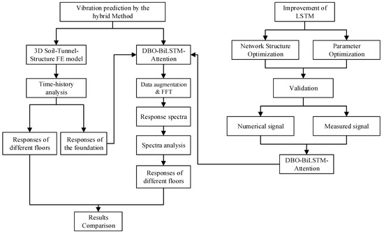
Figure 1.
Framework of proposed hybrid method.
Notes: LSTM-Long Short-Term Memory; FFT-Fast Fourier Transform; DBO-Dung Beetle Optimizer
- (1)
- LSTM Model Improvement
The first step focuses on improving the LSTM model, which involves both network structure refinement and parameter tuning. In this step, a DBO–BiLSTM–attention model is developed, which integrates multiple advanced features for improved performance. The improvement ensures accurate predictions while capturing the temporal and sequential characteristics of the data.
① Network Structure Improvement
The LSTM model is enhanced by incorporating BiLSTM layers, which enable the model to capture sequential dependencies in both forward and backward directions. This bidirectional feature improves the ability of the model to identify patterns in the time-series vibration data.
② Parameter Optimization Using Dung Beetle Optimizer (DBO) Algorithm
The DBO algorithm is applied to fine-tune the hyperparameters of the BiLSTM network, such as the number of layers, learning rate, and size of hidden units. DBO ensures the efficient exploration of the parameter space, leading to better model convergence and generalization.
③ Attention Mechanism Integration
A self-attention mechanism is integrated into the model to prioritize critical time steps or features in the vibration data. By focusing on the most relevant parts of the signal, the attention mechanism enhances the model’s ability to predict subtle changes in vibration characteristics.
④ Validation by Simulation Signal and Measured Signal
We used the numerical simulation signal and real-world subway-induced vibration signal to validate the feasibility of the DBO–BiLSTM–attention model. It is worth noting that this dual-validation approach provides a more comprehensive assessment of the algorithm’s feasibility and effectiveness.
- (2)
- Vibration Prediction by the Hybrid Method
This DBO–BiLSTM–attention model is employed to augment the excitation signals. The time-history analysis and spectral analysis are used to obtain the structural responses. This process involves the following key steps:
① Development of 3D Soil–Tunnel–Structure Model
A 3D numerical model is developed to represent the interaction between the soil, tunnel, and overlying structures. This model incorporates material properties, boundary conditions, and the geometric configurations of the specific engineering case, ensuring an accurate simulation of vibration propagation and the corresponding structural response.
② Time-history Analysis
By utilizing the time-history analysis method, the vibration response induced by subway operations on nearby buildings is analyzed. The acceleration responses at the structure’s foundation and at different floors are obtained. It is worth noting that the acceleration responses at the structure’s foundation are used as the excitation signals in the next step.
③ Fast Fourier Transform (FFT) of Excitation Signals
The excitation signals are augmented using the DBO–BiLSTM–attention model. And then FFT is applied to convert the time-domain data into the frequency domain, generating response spectra that characterize the vibrational energy distribution.
④ Spectral analysis
The response spectra derived from the excitation signals are used as input for the spectral analysis. The spectral analysis is conducted to calculate the maximum acceleration responses of the structure.
⑤ Comparison with Time-History Method
To validate the effectiveness of the proposed method, the results of the spectral analysis are compared to the outcomes obtained using the time-history analysis method.
3. Improvement of LSTM Model
LSTM is a type of RNN specifically designed to overcome the shortcomings of traditional RNNs, such as the vanishing gradient problem, which makes it difficult for RNNs to learn long-term dependencies in sequences. LSTM was introduced by Hochreiter and Schmidhuber in 1997 [29] and has since become a powerful tool for sequential data modeling, particularly in fields like time-series prediction, speech recognition, and natural language processing.
3.1. RNNs and the Vanishing Gradient Problem
Recurrent Neural Networks (RNNs) are designed to process sequences by maintaining hidden states that depend on previous inputs. At each time step t, an RNN processes the input xt and updates its hidden state ht using the following equation:
where Wh and Wx are weight matrices, b is the bias term, and f is the activation function, typically a tanh or sigmoid function. While this approach works for short sequences, RNNs encounter difficulties when dealing with long-range dependencies. The vanishing gradient problem arises during backpropagation through time (BPTT), where gradients become very small as they are propagated backward through multiple time steps, making it difficult for the model to learn long-term dependencies.
3.2. The LSTM Model
The LSTM model is an extension of the traditional RNN designed to overcome this problem. The key innovation in LSTMs is the memory cell, which serves as a long-term storage unit that can preserve information over extended periods of time. This cell is controlled by three gating mechanisms: the forget gate, the input gate, and the output gate. These gates allow the LSTM to selectively retain or forget information at each time step, addressing the limitations of standard RNNs [29]. The basic structure of LSTM is shown in Figure 2.
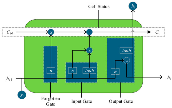
Figure 2.
Basic structure of LSTM.
3.2.1. Memory Cell
The memory cell Ct is responsible for storing information over time. The LSTM updates its memory cell at each time step based on the current input xt and the previous hidden state ht−1. The cell state is updated according to the following equation:
where Ct is the current cell state, ft is the forget gate output, Ct−1 is the previous cell state, it is the input gate output, and is the candidate cell state, which represents the new information to be added to the cell state.
3.2.2. Gates in LSTM
The LSTM employs three key gates that control the flow of information:
Forgotten Gate (ft): It decides what proportion of the previous cell state Ct−1 should be carried forward. It is computed as follows:
where σ is
the sigmoid activation function; Wf and bf
are learnable parameters.
Input Gate (it): It determines how much new information should be added to the memory cell. It is given by
Output Gate (ot): It controls how much of the cell state should be output as the hidden state. The output gate is computed as
The final hidden state ht is calculated as
where tan h is the hyperbolic tangent activation function, which ensures that the hidden state is bounded between −1 and 1.
3.2.3. Evaluation Metrics
To evaluate the performance of the LSTM model, Mean Absolute Error (MAE), Root Mean Square Error (RMSE), and Coefficient of Determination (R2) key metrics are commonly used key metrics. These metrics provide a quantitative assessment of the model’s predictive accuracy and overall reliability.
where and are the actual and predicted values, respectively.
3.3. LSTM Model Improvement
3.3.1. Network Structure Improvement
In this study, the LSTM network is enhanced in two steps to improve its predictive performance and reduce errors. The first step involves replacing the standard unidirectional LSTM network with a Bidirectional LSTM (BiLSTM) network. The second step incorporates an attention layer into the BiLSTM architecture, forming a BiLSTM–attention network. The details of these two improvements are as follows:
- (1)
- Replacement of unidirectional LSTM with BiLSTM
Traditional LSTM networks process sequential data in a unidirectional manner, relying solely on past information to predict future outputs. However, many real-world time-series datasets exhibit dependencies not only on historical states but also on future states. To address this limitation, a Bidirectional Long Short-Term Memory (BiLSTM) network is employed as a replacement for the standard unidirectional LSTM. BiLSTM combines a forward LSTM and a backward LSTM, allowing it to process data in both temporal directions. This dual-perspective processing enables the model to capture bidirectional dependencies within sequential data more effectively. The forward LSTM processes the input sequence from past to future, while the backward LSTM processes the sequence in reverse order, ensuring that both past and future contexts contribute to the prediction [30]. The BiLSTM structure is depicted in Figure 3.
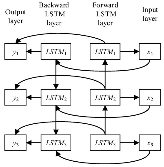
Figure 3.
Structure of BiLSTM.
- (2)
- Integration of attention mechanism
While BiLSTM effectively captures bidirectional dependencies, the relationships between different parts of the input sequence may still be underutilized. To address this issue, an attention mechanism is introduced into the BiLSTM architecture. Specifically, a self-attention mechanism is added, which proved effective in highlighting the most relevant parts of the input sequence and uncovering the intrinsic relationships within the data. The self-attention mechanism calculates a weighted representation of the input sequence, where the importance of each input element is determined by learned attention scores. Unlike traditional attention mechanisms that rely on external information, self-attention derives the Query, Key, and Value vectors from the same input sequence. This characteristic reduces the model’s dependency on external data and allows it to focus entirely on discovering internal relationships [31]. The structure of the self-attention mechanism is shown in Figure 4.
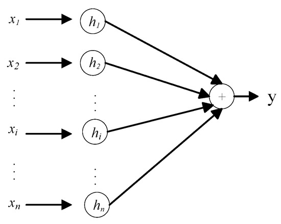
Figure 4.
Structure of self-attention mechanism.
The attention layer is integrated on top of the BiLSTM network, forming the BiLSTM–attention model. This structure enhances the network’s ability to assign different levels of importance to input elements, enabling more accurate predictions [30]. The structure of the BiLSTM–attention network is illustrated in Figure 5.
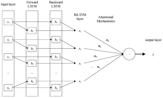
Figure 5.
Structure of BiLSTM–attention model.
3.3.2. Parameter Optimization Using DBO Algorithm
Parameter settings have a significant impact on the predictive performance of machine learning models. Manual parameter tuning is often subjective and imprecise, resulting in suboptimal outcomes. To address this issue, this study integrates the Dung Beetle Optimizer (DBO) [32] into a BiLSTM–attention network to achieve automatic hyperparameter optimization. The DBO simulates the natural behaviors of dung beetles, including rolling, foraging, navigating, mating, and stealing, to efficiently explore and exploit the parameter space. By optimizing key parameters such as the number of hidden units, maximum training epochs, and initial learning rate, the proposed DBO–BiLSTM–attention framework significantly enhances model accuracy and robustness.
The specific settings for the DBO algorithm in this study are as follows—population size: 30; maximum number of iterations: 10; lower bounds for parameters: [15 (hidden units), 30 (training epochs), 0.001 (learning rate)]; upper bounds for parameters: [150 (hidden units), 500 (training epochs), 0.1 (learning rate)].
3.4. Model Performance Validation
3.4.1. Simulation Signal Validation
- (1)
- Signal characteristics
To compare the performance of the LSTM model before and after improvement, the simulation signal was firstly used for validation. The signal is generated by combining sine and cosine functions, as shown in the following equation:
where the signal frequency f = 10 Hz, the sampling frequency Fs is 1000 Hz, the sampling time is 1 s, and there are 1000 sample points. Considering that the real-world measured signals contain varying levels of noise, four different levels (5%, 10%, 15%, and 20%) of Gaussian white noise are added to the simulated signal to mimic the actual conditions.
- (2)
- Prediction results
The model parameters were chosen with a training-to-testing dataset ratio of 0.7, a sliding window of 10, one-step prediction, 1000 training iterations, 128 hidden layer neurons, and one fully connected layer. The optimizer used was Adam. LSTM, BiLSTM, and DBO–BiLSTM–attention models were used for data prediction. The prediction results under four different operating conditions are shown in Figure 6, Figure 7, Figure 8 and Figure 9. The prediction results from different models are very close. However, noticeable differences emerge in the local rising segments. The prediction results from the DBO–BiLSTM–attention network are closer to the original signal trend compared to the other models.
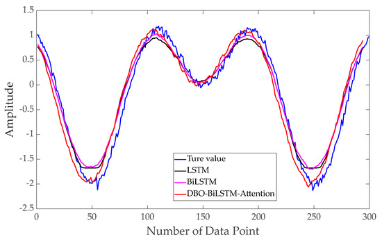
Figure 6.
Prediction results of scenario 1: Noise level of 5%.
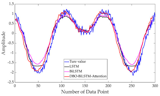
Figure 7.
Prediction results of scenario 2: Noise level of 10%.
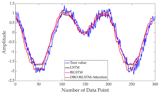
Figure 8.
Prediction results of scenario 3: Noise level of 15%.
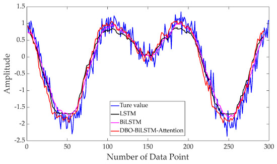
Figure 9.
Prediction results of scenario 4: Noise level of 20%.
The evaluation metric values of different models under different noise levels are shown in Table 1. As the noise level increases, the prediction errors of all models increase as well, but the DBO–BiLSTM–attention model still maintains the highest accuracy. Especially in scenario 4, the RMSE of the DBO–BiLSTM–attention network decreased by 13.1% compared to the original LSTM network, the MAE decreased by 12.7%, and the R2 improved by 3.20%.

Table 1.
Evaluation metric values of different models under different noise levels.
3.4.2. Real-World Measured Signal Validation
- (1)
- Data collection for subway-induced vibrations
The acceleration signals used in this study were obtained from data collected by Wang et al. [33], who investigated subway-induced vibrations and the influence on nearby building structures. Acceleration sensors, type 1A212E, and a DH8303 dynamic signal testing and analysis system were employed for data measurement. The sampling frequency was set to 1000 Hz, which is sufficiently high to cover the full spectrum of subway-induced vibration frequencies. This configuration ensured that the collected signals comprehensively represented the vibrational impact of subway operations on the surrounding environment, providing high-quality data for subsequent analyses.
A total of six monitoring points were arranged on the ground surface, as illustrated in Figure 10. When a train passes, the train operation can induce vibrations in the ground surface. In order to understand the influence of vibrations on the ground at different distances from the subway tunnel, measurement points were arranged according to varying distances, and vibration signals induced by subway operation were collected. The positions of the monitoring points were as follows—(1) Point 1: Located centrally between the two subway tunnels. (2) Points 2 to 6: Positioned progressively farther from Point 1 at distances of 1 m, 2 m, 4 m, 6 m, and 20 m, respectively.
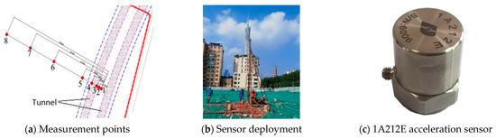
Figure 10.
Layout of measurement points.
The measured acceleration time history and corresponding frequency spectrum for Point 1 are presented in Figure 11. The time history captures the temporal variations in ground acceleration caused by subway train passage, while the frequency spectrum reveals the distribution of vibrational energy across different frequencies.
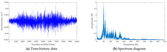
Figure 11.
Measured data of Point 1.
- (2)
- Prediction results
In this section, the prediction performance of the proposed models is validated using real-world vibration signals. The same network parameters as described in Section 3.4.1 are applied to predict the signal for measurement Point 1. The results are shown in Figure 12, Figure 13 and Figure 14. It can be observed that the predictions from the DBO–BiLSTM–attention model closely match the real-world measured signals, effectively replicating the frequency-domain range covered by the actual measured signal.
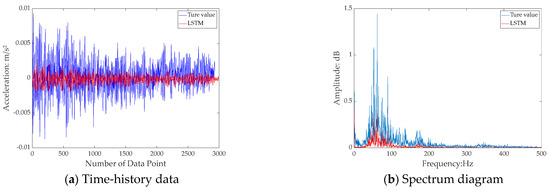
Figure 12.
Prediction results by LSTM.
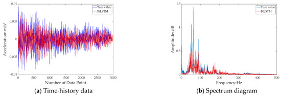
Figure 13.
Prediction results by BiLSTM.
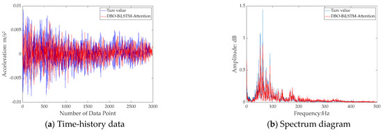
Figure 14.
Prediction results by DBO–BiLSTM–attention.
The error statistics results are shown in Table 2, where the DBO–BiLSTM–attention model demonstrates the most significant performance improvement. Compared to the LSTM network, RMSE decreased by 67.2%, MAE decreased by 67.9%, and R2 increased by 49.37%. Therefore, it can be concluded that the DBO–BiLSTM–attention model can also make relatively accurate predictions for measured signals.
Table 2.
Evaluation metric values of different models.
4. Validation of Hybrid Method
In Section 3.4.2, due to the lack of accurate information of soil layers and nearby building structures in the field, it is challenging to use the real-world measured signals to validate the proposed hybrid method. Therefore, a numerical simulation is used to validate the hybrid method in this section, and a flowchart is shown in Figure 15.
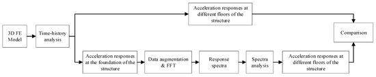
Figure 15.
The flowchart of the validation.
(1) FE Model: Using Midas GTS NX 2021 finite element software, a 3D soil–tunnel–structure model is developed. The parameters of soil layers and materials are defined, and the load functions as well as the loading points are specified.
(2) Time-history Analysis: By utilizing the time-history analysis method, the vibration response induced by subway operations on nearby buildings is analyzed. The acceleration responses at the structure’s foundation and at different floors are determined.
(3) Spectral Analysis: The DBO–BiLSTM–attention model is employed to augment the acceleration signals obtained at the structure’s foundation in Step (2). FFT is performed on both the original and augmented signals to generate the corresponding response spectra. These two different spectra are then used as inputs to calculate the maximum acceleration response of the structure. The results are compared with the baseline values obtained by the time-history analysis in Step (2).
4.1. FE Model
The FE model is illustrated in Figure 16. The dimensions are 100 m × 100 m × 50 m. For the sake of computational simplicity, the soil layers are represented as a homogeneous soil body. The above-ground structure is a three-story tower, with a total height of 10 m and inter-floor heights of 4 m, 3 m, and 3 m, respectively. The soil layers and tower are modeled by using 3D solid elements. The tunnel has a diameter of 6 m and a lining thickness of 0.6 m. In Midas GTS NX, when meshing the 3D model of the soil–tunnel–structure, the first step is to select appropriate mesh generation methods (such as 3D automatic solid mesh) for the tunnel, soil layers, and structure, respectively, and specify suitable seeding methods and mesh sizes. Then, use the automatic mesh generation function to generate the meshes for the tunnel, soil layers, and building, and perform necessary optimizations and checks to ensure that the mesh interior coupling is correct and there are no overlapping or broken mesh elements. Finally, name and group the generated meshes for a subsequent analysis and management.
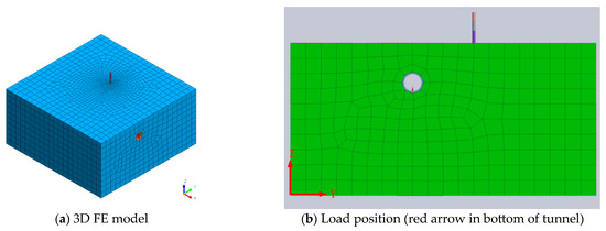
Figure 16.
FE model.
The material parameters of each component are provided in Table 3.
Table 3.
Material parameters of each component.
4.2. Time-History Analysis
A direct time-history analysis is a time-history analysis method based on the principles of a dynamic finite element analysis. It calculates the dynamic response of a structure under a given load by directly inputting the load acceleration time history into the model. In Midas GTS NX, a direct time-history analysis can be applied to a vibration response analysis of various structures, including soil, tunnels, structures, and more. This method provides a more accurate simulation of the dynamic behavior of structures under load, albeit with a relatively larger computational burden.
4.2.1. Train Dynamic Loads
Train dynamic loads are critical in assessing the effects of train movements on the surrounding environment, including tunnels, tracks, and nearby structures. The train dynamic loads generated by subway operations exhibit inherent randomness, mainly due to factors such as local track irregularities, the spacing and arrangement of rail ties, and eccentric wheel loads. However, some factors (such as train speed and wheel–rail spacing) remain constant; there are also constant components within the vibration loads. Therefore, the excitation force function (shown in Equation (12)) can be used to simulate the dynamic load of the train. This equation includes both static loads and dynamic loads iterated from a series of sine functions [34,35].
where represents the static wheel load; , , and correspond to the peak load values associated with the typical vertical displacement αi of the rail vibrations, respectively. t represents the time during which the load is applied. can be calculated using the following equation:
where m is the sprung mass of the vehicle, and is the angular frequency, calculated as
where v represents the train speed, and the parameter values are shown in Table 4.
Table 4.
Parameter values of train dynamic loads.
The train dynamic load is applied at the bottom of the tunnel by defining a time-dependent load function in Midas GTS NX, as shown in Figure 16b. In this study, a train speed of 40 km/h is selected. When v = 40 km/h, the train takes 10 s to pass through. Therefore, the total duration is set to 10 s. To assess the influence of different data lengths on prediction accuracy, sampling frequencies (Fs) of 100 Hz, 200 Hz, and 300 Hz are set. The number of sample points obtained is 1000, 2000, and 3000, respectively.
4.2.2. Results
A point selected at the structural foundation is labeled as Point 1#. Additional points are chosen at the heights of 4 m, 7 m, and 10 m in the structure, and are labeled as Points 2#, 3#, and 4#, respectively. The locations and maximum acceleration response values of the four points are shown in Figure 17.
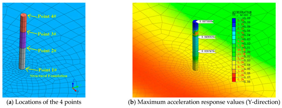
Figure 17.
The diagram of the point locations and responses.
By the time-history analysis, the dynamic responses of the structure at Points 1# to 4# under different sampling frequencies are obtained. This study focuses exclusively on the acceleration response in the Y-direction. Due to space limitations, only the time-history of the acceleration response at Point 1# (structural foundation) is presented. The Y-direction acceleration responses at Point 1# are shown in Figure 18, used as the input for the spectral analysis in the next section. Point 1#, situated at the structural foundation, exhibits notable fluctuations in the first half of the graph, primarily attributed to instantaneous vibrations induced by load activation. Over time, the acceleration at Point 1# gradually stabilizes and exhibits regular oscillations.
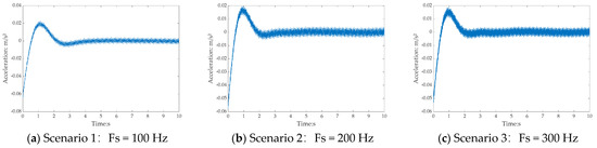
Figure 18.
Dynamic responses at Point 1# (structural foundation).
Figure 19 illustrates the maximum acceleration values of different floors (Points 2# to 4#). Notably, the maximum acceleration values at Points 2 to 4 remain relatively consistent across the three scenarios. However, due to the combined effects of factors such as mass distribution and the structure’s vibration modes, the acceleration values at Points 2# to 4# exhibit a distinct pattern, increasing progressively with height.
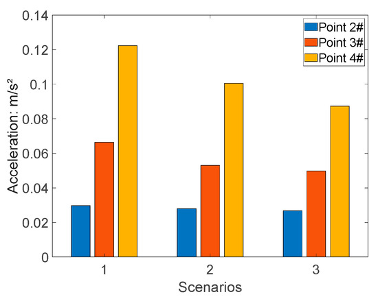
Figure 19.
Acceleration at Points 2# to 4# under different scenarios.
4.3. Spectral Analysis
4.3.1. Data Augmentation
The acceleration response data at Point 1# (structural foundation) are selected as the excitation signal for the spectral analysis. Both the original and augmented signals are used to generate the corresponding response spectra. An additional 50% data augmentation is performed using the DBO–BiLSTM–attention model. The results are shown in Figure 20 and Figure 21, and the detailed errors are provided in Table 5.
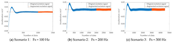
Figure 20.
Comparison of time-history data of original excitation signal and augmented excitation signal.
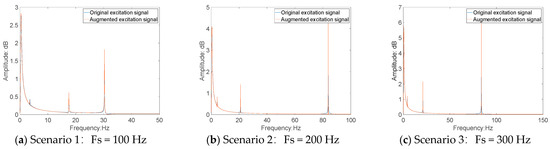
Figure 21.
Comparison of frequency spectrum of original excitation signal and augmented excitation signal.
Table 5.
Prediction errors of different Scenarios.
As shown in Figure 20 and Figure 21 and Table 5, the predicted values from the DBO–BiLSTM–attention model closely match the actual values. As the amount of training data increase, the prediction errors, represented by RMSE and MAE, gradually decrease, and the goodness of fit improves, with the R2 value progressively approaching 1.0. This indicates that a larger dataset leads to better prediction performance. Therefore, data augmentation using this model is a reliable approach.
4.3.2. Results
The FFT is applied to both the original excitation signal and the augmented excitation signal from Section 4.2.2 to obtain the corresponding response spectra. These spectra are then input into Midas GTS NX 20201, with Point 1# (the structural foundation) designated as the excitation point for the spectral analysis. Due to space limitations, only the Y-direction acceleration contour map of the structure under scenario 1 is shown in Figure 22.
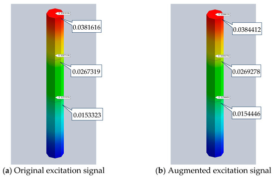
Figure 22.
The Y-direction acceleration contour map of the structure in scenario 1 (unit: m/s2).
Using the maximum acceleration response values derived from the time-history analysis in Section 4.2.2 as a baseline, Table 6 presents a comparison between the results obtained using the original excitation signal and those derived from the augmented excitation signal. The frequency difference between the results obtained from two types of input data and the baseline is shown in Figure 23. It can be observed that the errors in both cases are nearly identical, and overall, the error decreases as the number of sample points increases. This indicates that increasing the number of sample points for data augmentation effectively reduces the error. The maximum prediction error occurs in scenario 1 of Point 4#. The maximum difference between “baseline” and “original” is 0.015 m/s2. The maximum difference between “baseline” and “augmented” is 0.009 m/s2. Applying the proposed hybrid method for data augmentation enhances the accuracy of the spectral analysis. The hybrid method proposed achieves an improvement of 7% for the prediction accuracy.
Table 6.
Results derived from original excitation signal and augmented excitation signal (Unit: m/s2).
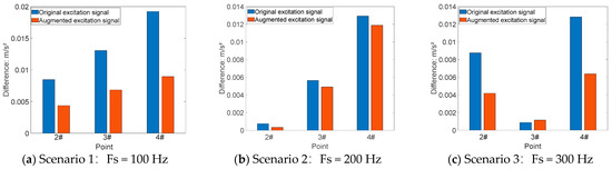
Figure 23.
The frequency difference between the results obtained from two types of input data and the baseline.
5. Conclusions
This paper proposes a hybrid method for predicting structural vibration responses induced by subway operations by combining improved LSTM and a spectral analysis. The main conclusions are as follows:
(1) The improved LSTM model is composed of BiLSTM, an attention mechanism, and the DBO algorithm, resulting in the development of the DBO–BiLSTM–attention network. This model is validated using both numerical simulation signals and measured signals. The results show a significant improvement in prediction accuracy compared to the standard LSTM network. For numerical simulation signals, values of RMSE and MAE decreased to varying degrees under different scenarios, while the value of R2 increased by at least 3% while maintaining a high level. For the measured data of subway-induced vibration, RMSE decreased by 67.2%, MAE decreased by 67.9%, and R2 increased by 49.37%.
(2) For the hybrid method, validation results from numerical simulation cases indicate that the structural acceleration response values obtained using the proposed hybrid method closely match those derived from the time-history analysis method. Additionally, as the amount of input data increases, the error decreases. Applying the proposed hybrid method for data augmentation enhances the accuracy of the spectral analysis. The hybrid method proposed achieves an improvement of 7% for the prediction accuracy.
(3) Limitations and future work: The validation of the hybrid method in this study is based on numerical simulations and lacks validation using real-world engineering data. Future research should focus on further validation and application in practical engineering projects.
Author Contributions
Conceptualization, X.L., G.X., and X. Ye; methodology, G.X.; validation, X.L. and X.Y.; formal analysis, X.L.; investigation, X.L. and G.X.; resources, X.Y.; data curation, X.L. and G.X.; writing—original draft preparation, X.L.; writing—review and editing, G.X. and X.Y.; visualization, X.L.; supervision, G.X. and X.Y. All authors have read and agreed to the published version of the manuscript.
Funding
This research received no external funding.
Institutional Review Board Statement
Not applicable.
Informed Consent Statement
Not applicable.
Data Availability Statement
All models, or code, that support the findings of this study are available from the corresponding author upon reasonable request.
Conflicts of Interest
The authors declare no conflicts of interest.
References
- Xu, D.; Zhao, Y.; Liu, H.; Zhu, H. Deformation monitoring of metro tunnel with a new ultrasonic-based system. Sensors 2017, 17, 1758. [Google Scholar] [CrossRef] [PubMed]
- Kurzweil, L.G. Ground-borne noise and vibration from underground rail systems. J. Sound Vib. 1979, 66, 363–370. [Google Scholar] [CrossRef]
- Melke, J. Noise and vibration from underground railway lines: Proposals for a prediction procedure. J. Sound Vib. 1988, 120, 391–406. [Google Scholar] [CrossRef]
- Madshus, C.; Kaynia, A.M. High-speed railway lines on soft ground: Dynamic behavior at critical train speed. J. Sound Vib. 2000, 231, 689–701. [Google Scholar] [CrossRef]
- Bahrekazemi, M. Train-Induced Ground Vibration and Its Prediction. Ph.D. Thesis, Royal Institute of Technology, Stockholm, Sweden, 2004. [Google Scholar]
- Tao, Z.; Moore, J.A.; Sanayei, M.; Wang, Y.; Zou, C. Train-induced floor vibration and structure-borne noise predictions in a low-rise over-track building. Eng. Struct. 2022, 255, 113914. [Google Scholar] [CrossRef]
- Kedia, N.K.; Kumar, A.; Singh, Y. Development of Empirical Relations to Predict Ground Vibrations due to Underground Metro Trains. KSCE J. Civ. Eng. 2023, 27, 251–260. [Google Scholar] [CrossRef]
- Gupta, S.; Degrande, G.; Lombaert, G. Experimental validation of a numerical model for subway induced vibrations. J. Sound Vib. 2009, 321, 786–812. [Google Scholar] [CrossRef]
- Amado-Mendes, P.; Costa, P.A.; Godinho, L.M.; Lopes, P. 2.5D MFS–FEM model for the prediction of vibrations due to underground railway traffic. Eng. Struct. 2015, 104, 141–154. [Google Scholar] [CrossRef]
- Bian, X.; Hu, J.; Thompson, D.; Powrie, W. Pore pressure generation in a poro-elastic soil under moving train loads. Soil Dyn. Earthq. Eng. 2019, 125, 105711. [Google Scholar] [CrossRef]
- Qu, S.; Yang, J.; Zhu, S.; Zhai, W.; Kouroussis, G. A hybrid methodology for predicting train-induced vibration on sensitive equipment in far-field buildings. Transp. Geotech. 2021, 31, 100682. [Google Scholar] [CrossRef]
- Wu, Z.; Zhang, N.; Bi, W.; Liu, J. Application of FEM–BEM–PEM Hybrid Random-Vibration Method on Low-Frequency Structure-Borne Noise Prediction of U-Shaped Girder in Urban Rail Transit. Int. J. Struct. Stab. Dyn. 2024. [Google Scholar] [CrossRef]
- Costa, P.A.; Calçada, R.; Cardoso, A.S. Track–ground vibrations induced by railway traffic: In-situ measurements and validation of a 2.5D FEM-BEM model. Soil Dyn. Earthq. Eng. 2012, 32, 111–128. [Google Scholar] [CrossRef]
- Liu, W.; Wu, Z.; Li, C.; Xu, L. Prediction of ground-borne vibration induced by a moving underground train based on excitation experiments. J. Sound Vib. 2022, 523, 116728. [Google Scholar] [CrossRef]
- He, C.; Zhou, S.; Di, H.; Zhang, X. An efficient prediction model for vibrations induced by underground railway traffic and experimental validation. Transp. Geotech. 2021, 31, 100646. [Google Scholar] [CrossRef]
- Colaço, A.; Castanheira-Pinto, A.; Costa, P.A.; Ruiz, J.F. Combination of experimental measurements and numerical modelling for prediction of ground-borne vibrations induced by railway traffic. Constr. Build. Mater. 2022, 343, 127928. [Google Scholar] [CrossRef]
- Shu, J.; Yu, H.; Liu, G. DF-CDM: Conditional diffusion model with data fusion for bridge dynamic response reconstruction. Mech. Syst. Signal Process. 2024, 222, 111783. [Google Scholar] [CrossRef]
- Wang, S.; Lin, S.; Yang, R. A lightweight convolutional neural network for multipoint displacement measurements on bridge structures. Nonlinear Dyn. 2024, 112, 11745–11763. [Google Scholar] [CrossRef]
- Sun, R.; Wang, S.; Li, M.; Zhu, Y. An algorithm for large-span flexible bridge pose estimation and multi-key point vibration displacement measurement. Measurement 2024, 240, 115582. [Google Scholar] [CrossRef]
- Wang, S.; He, J.; Fan, J.; Sun, P.; Wang, D. A time-domain method for free vibration responses of an equivalent viscous damped system based on a complex damping model. J. Low Freq. Noise Vib. Act. Control. 2023, 42, 1531–1540. [Google Scholar] [CrossRef]
- He, Y.; Zhang, Y.; Yao, Y.; He, Y.; Sheng, X. Review on the Prediction and Control of Structural Vibration and Noise in Buildings Caused by Rail Transit. Buildings 2023, 13, 2310. [Google Scholar] [CrossRef]
- Liang, R.; Liu, W.; Li, C.; Li, W.; Wu, Z. A novel efficient probabilistic prediction approach for train-induced ground vibrations based on transfer learning. J. Vib. Control 2024, 30, 576–587. [Google Scholar] [CrossRef]
- Abbas, N.; Umar, T.; Salih, R.; Akbar, M.; Hussain, Z.; Haibei, X. Structural Health Monitoring of Underground Metro Tunnel by Identifying Damage Using ANN Deep Learning Auto-Encoder. Appl. Sci. 2023, 13, 1332. [Google Scholar] [CrossRef]
- Siłka, J.; Wieczorek, M.; Woźniak, M. Recurrent neural network model for high-speed train vibration prediction from time series. Neural Comput. Applic 2022, 34, 13305–13318. [Google Scholar] [CrossRef]
- Zhang, Y.; Xie, X.; Li, H.; Zhou, B.; Wang, Q.; Shahrour, I. Subway tunnel damage detection based on in-service train dynamic response, variational mode decomposition, convolutional neural networks and long short-term memory. Autom. Constr. 2022, 139, 104293. [Google Scholar] [CrossRef]
- Xin, T.; Yang, Y.; Zheng, X.; Lin, J.; Wang, S.; Wang, P. Time Series Recovery Using Adjacent Channel Data Based on LSTM: A Case Study of Subway Vibrations. Appl. Sci. 2022, 12, 11497. [Google Scholar] [CrossRef]
- Li, S.; Qiu, Y.; Jiang, J.; Wang, H.; Nan, Q.; Sun, L. Identification of Abnormal Vibration Signal of Subway Track Bed Based on Ultra-Weak FBG Sensing Array Combined with Unsupervised Learning Network. Symmetry 2022, 14, 1100. [Google Scholar] [CrossRef]
- Jie, L.; Fang, L.; Weiping, X.; Xiaoxiong, J. Track vibration sequence anomaly detection algorithm based on LSTM. Adv. Struct. Eng. 2023, 26, 1682–1695. [Google Scholar] [CrossRef]
- Hochreiter, S.; Schmidhuber, J. Long short-term memory. Neural Comput. 1997, 9, 1735–1780. [Google Scholar] [CrossRef] [PubMed]
- Hao, X.; Liu, Y.; Pei, L.; Li, W.; Du, Y. Atmospheric Temperature Prediction Based on a BiLSTM Attention Model. Symmetry 2022, 14, 2470. [Google Scholar] [CrossRef]
- Kim, T.Y.; Cho, S.B. Predicting residential energy consumption using CNN-LSTM neural networks. Energy 2019, 182, 72–81. [Google Scholar] [CrossRef]
- Shen, B.; Liu, Y.; Chen, H.; Yu, Y. Dung Beetle Optimizer: A New Swarm Intelligence Algorithm for Global Optimization. Appl. Soft Comput. 2022, 130, 109703. [Google Scholar]
- Wang, D.; Liang, Q.; Zhou, Y.; Li, J.; Ke, X.; Ling, H.; Ding, C. Study on vertical shaking table model test of super high-rise structure over subway: Engineering background and model verification. Build. Struct. 2022, 52, 1–8, 28. (In Chinese) [Google Scholar]
- Pan, C.; Pande, G.N. Preliminary deterministic finite element study on a tunnel driven in loess subjected to train loading. China Civ. Eng. J. 1984, 17, 19–28. (In Chinese) [Google Scholar]
- Lai, J.; Zhou, H.; Wang, K.; Qiu, J.; Wang, L.; Wang, J.; Feng, Z. Shield-driven induced ground surface and Ming Dynasty city wall settlement of Xi’ an metro. Tunn. Undergr. Space Technol. 2020, 97, 103220. [Google Scholar] [CrossRef]
Disclaimer/Publisher’s Note: The statements, opinions and data contained in all publications are solely those of the individual author(s) and contributor(s) and not of MDPI and/or the editor(s). MDPI and/or the editor(s) disclaim responsibility for any injury to people or property resulting from any ideas, methods, instructions or products referred to in the content. |
© 2025 by the authors. Licensee MDPI, Basel, Switzerland. This article is an open access article distributed under the terms and conditions of the Creative Commons Attribution (CC BY) license (https://creativecommons.org/licenses/by/4.0/).