NHSH: Graph Hybrid Learning with Node Homophily and Spectral Heterophily for Node Classification

Abstract

Graph Neural Network (GNN) is an effective model for processing graph-structured data. Most GNNs are designed to solve homophilic graphs, where all nodes belong to the same category. However, graph data in real-world applications are mostly heterophilic, and homophilic GNNs cannot handle them well. To address this, we propose a novel hybrid-learning framework based on Node Homophily and Spectral Heterophily (NHSH) for node classification in graph networks. NHSH is designed to achieve state-of-the-art or superior performance on both homophilic and heterophilic graphs. It includes three core modules: homophilic node extraction (HNE), heterophilic spectrum extraction (HSE) and node feature fusion (NFF). More specifically, HNE identifies symmetric neighborhoods of nodes with the same category, extracting local features that reflect these symmetrical structures. Then, HSE uses filters to analyze the high and low-frequency information of nodes in the graph and extract the global features of the nodes. Finally, NFF fuses the above two node features to obtain the final node features in graphs. Moreover, an elaborate loss function drives the network to preserve critical symmetries and structural patterns in the graph. Experiments on eight benchmark datasets validate that NHSH performs comparably or better than existing methods across diverse graph types.

1. Introduction

In recent years, graph neural networks (GNNs) have become a hot research topic because of their good performance on various downstream tasks, such as node classification, link prediction, graph classification, etc. For homophilic graphs, where nodes of the same category tend to be connected, GNNs can integrate semantic and contextual information into node embeddings [1,2,3,4,5], as shown in Figure 1a,b. These connections often exhibit a form of structural symmetry, where nodes with similar properties tend to form symmetric neighborhoods, which GNNs leverage to learn effective representations. However, there are a large number of heterophilic graphs where nodes of different categories are often connected in real-world application scenarios [6,7,8,9]. In these graphs, the connection patterns do not follow the same symmetry seen in homophilic graphs, creating additional complexity. For example, the biological protein topology is a typical heterophilic graph with different types of amino acid bonds, and different chemical effects can be produced by connecting different amino acid bonds. Therefore, how to implement competitive GNNs to efficiently process heterophilic graphs remains an open research topic.

In order to minimize the loss of feature information when updating nodes in heterophilic graphs, a weighted multi-hop strategy is used to find homophilic nodes in a heterophilic graph [10,11,12]. The filter-based method only aggregates the low-frequency and high-frequency information of the node [13,14]. Spectral information is less affected by local noise but tends to overlook the attributes of individual nodes. Furthermore, if only homophilic nodes are considered, the topological structure of the graph cannot be effectively used to update node features [15]. Therefore, only considering the spectrum information or the implicit homophilic node information in the heterophilic graph cannot fully update the node features, nor can it fully reveal the structural pattern of the heterophilic graph. The literature review is summarized in

Table 1. Literature review.

References	Problems Areas	Proposed Methods	Similarities with NHSH	Differences with NHSH
[1,2,3,4,5,15]	Homophilic graph	By integrating semantic and contextual information, the node aggregation problem in homophilic graphs is effectively addressed through the learning of node embeddings.	Both leverage the structural information of the graph, utilizing its structural symmetry to enhance the quality of node representations for improved node classification.	NHSH not only focuses on the node aggregation problem in homophilic graphs but also combines local homophilic information with global spectral heterophilic information, enabling better handling of the complexity of heterophilic graphs.
[6,7,8,9,10,11,12]	Heterophilic graph	A graph convolution or multi-hop aggregation strategy is employed to update node features, enabling better handling of the complex connectivity patterns in heterophilic graphs.	Both focus on effectively aggregating and updating node features in heterophilic graphs, aiming to improve information aggregation strategies and minimize the risk of node feature loss.
[13,14]	Heterophilic graph	Focusing on the filter-based method, which uses low-frequency and high-frequency information to process different features of nodes in the graph.	Both propose the aggregation of node features using filters.

.

In this paper, we propose a novel graph hybrid-learning framework based on Node Homophily and Spectral Heterophily (NHSH) to effectively aggregate vital information for node classification. More specifically, we introduce a homophilic node extraction (HNE) module, which is used to analyze the neighborhood information of nodes to find nodes with the same category and then extract the local features of nodes. Then, the heterophilic spectrum extraction (HSE) module uses filters to analyze the high- and low-frequency information of nodes in the graph and extract the global features of the nodes. Finally, the node feature fusion (NFF) module fuses the above two node features to obtain the final node features based on adaptive weight. The overall architecture is shown in Figure 2.

The main contributions in this paper are as follows:

• We design a graph hybrid-learning framework based on Node Homophily and Spectral Heterophily (NHSH) that can effectively aggregate the local and global information of nodes and improve the accuracy of node classification.
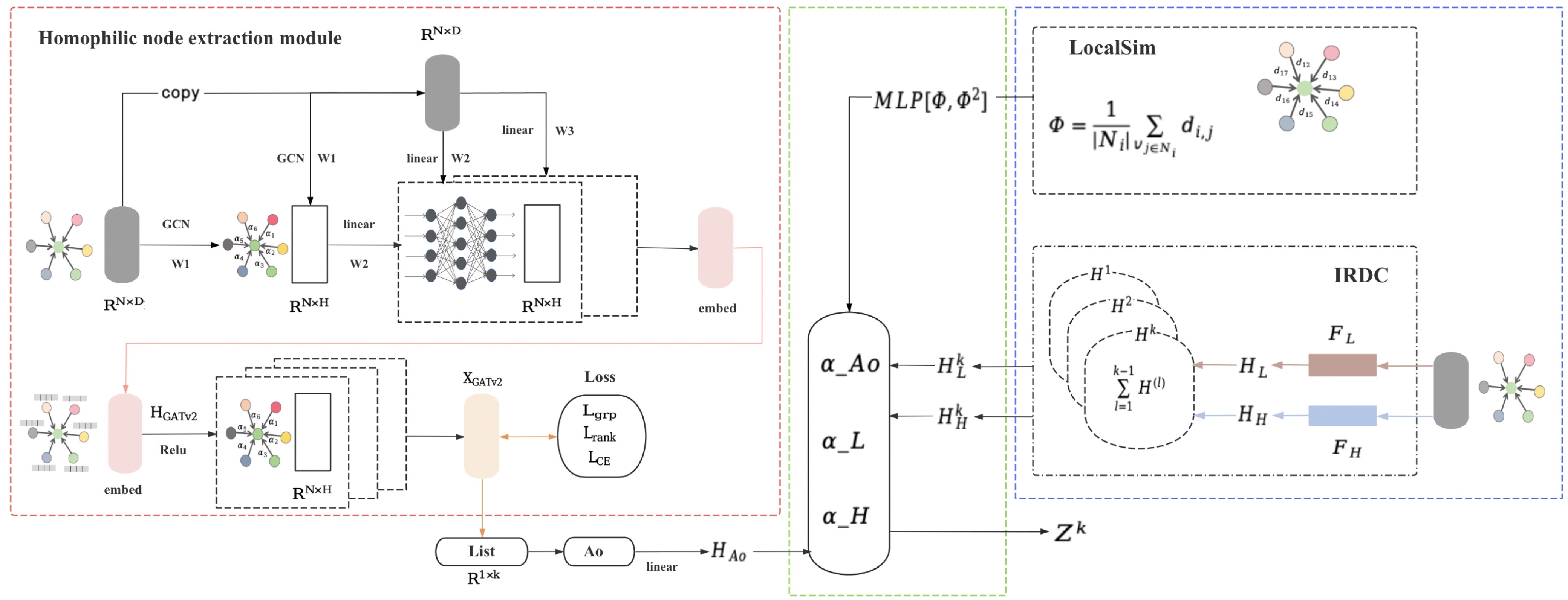
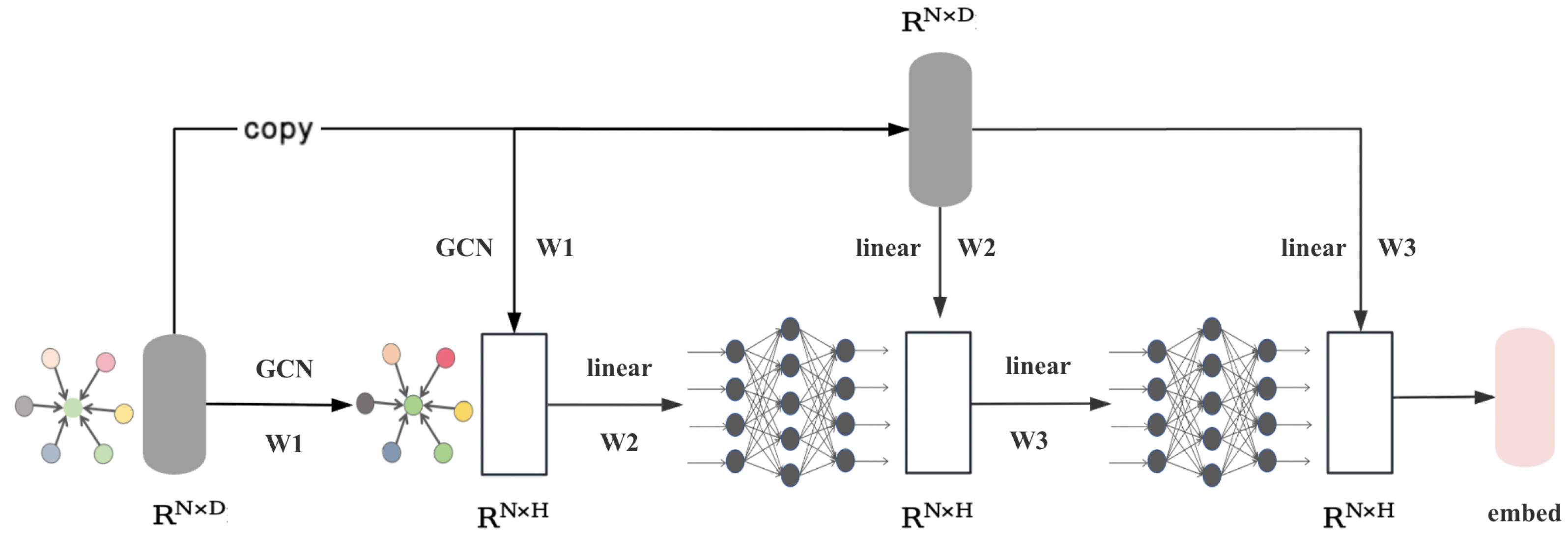
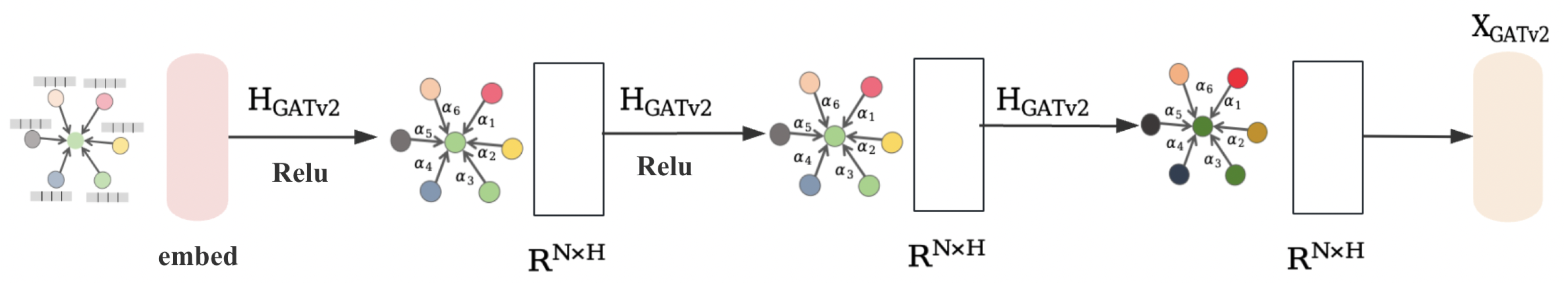
• The homophilic node extraction module combines graph convolutional network (GCN) and dynamic attention mechanism to find neighboring nodes with the same type as the central node to extract local features and obtain node homophily information. The heterophilic spectrum extraction module aggregates low- and high-frequency information from neighbors through low- and high-frequency filters to extract the global features of the nodes. The node feature fusion module uses the local topology information of the nodes to automatically generate fusion coefficients and dynamically update the final node features in graphs.
• Extensive experiments are implemented on eight benchmark datasets, demonstrating that the proposed network obtains competitive performances with eight state-of-the-art approaches in terms of quantitative comparisons.

The remainder of this paper is organized as follows. Section 2 introduces previous related works. In Section 3, we provide a detailed description of the proposed NHSH framework for node classification. Extensive experiments comparing eight methods across eight datasets are presented in Section 4. Finally, Section 5 shows the conclusion.

2. Related Works

2.1. Spectral-Based Graph Convolutional Networks

Spectral-based methods have a solid foundation in graph signal processing. Graphs are assumed to be undirected. Spectral GNN [16] treats the convolution kernel as a trainable matrix to directly capture the amplitude characteristics of the graph signal. However, this method requires the decomposition of the Laplacian matrix, which has a relatively high computational complexity. To solve this problem, ChebNet [13] defines a filter as Chebyshev polynomials of the diagonal matrix of eigenvalues, which implicitly avoids the computation of the graph Fourier basis, reducing the computational complexity. GCN [2] is known as the first-order approximation of ChebNet, where the graph convolution defined by 1stChebNet is local in space. It bridges the gap between spectral-based methods and spatial-based methods. It is considered to be a strong baseline in the research community due to its impressive performance in many node classification tasks. SGCN [17] is a further improvement of GCN. It reduces the complexity of GCN by eliminating nonlinearity and shows comparable or even better performance than GCN in various tasks. HLP [18] proposed a method using truncated singular value decomposition (TSVD) to exploit the topological structure of the graph as well as node features by modifying the aggregation strategy. GraphHeat [19] uses a heat kernel to design a more powerful low-pass filter. In addition, JacobiConv [20] discards nonlinearity and uses the Jacobi basis due to its orthogonality and flexibility to adapt to a wide range of weight functions. BernNet [21] learns arbitrary graph filters using Bernstein polynomials and is used to solve the heterophilic problem. GPRGNN [22] uses learnable negative and positive weights to aggregate features during message propagation, which is very suitable for processing heterophilic graphs because it can process both low-frequency and high-frequency components of graph signals. In summary, although spectral methods provide very clear interpretability in graph signal processing, they cannot provide a general solution for graph signals [5].

2.2. Spatial-Based Graph Convolutional Networks

Imitating the convolution operation of a conventional convolution neural network on an image, spatial-based methods define graph convolution based on a node’s spatial relations. For any graph, the spatial-based graph convolution aggregates the central node representation with its neighbor’s representation to obtain a new representation for the node [23,24]. GraphSAGE [5] generates embeddings for unseen nodes by training a set of aggregation functions, each of which aggregates information from different hops from a node. GAT [25] uses the attention mechanism to adaptively determine the weights of a node’s neighbors during aggregating feature information. MAMF-GCN [26] is proposed to better integrate features of modalities and different atlases by exploiting multi-channel correlation. PPNP [27] performs a linear transformation on node representation and then uses personalized pagerank to propagate information, which can retain the features of the node itself, but the computational cost is too high. Geo-CGN [28] uses graph embedding to transform discrete graphs into continuous geometric spaces, solving the problem of long-distance dependencies in graphs. H2GNN [14] aggregates neighbor information in a stacking manner to capture local and global information in the graph, alleviating the problem that it is difficult to distinguish different types of nodes as the number of network layers increases. MixHop [29] uses different adjacency power combinations to learn neighbor information of different distances to improve node representation capabilities. LnL-GNN [30] generates self-embedding based on the features of each node, defines two neighborhood types by calculating the mutual information between nodes, and uses a two-layer aggregation method to aggregate local and non-local neighborhood information to obtain node key features. CPGNN [31] introduces a compatibility matrix to model the homophily and heterophily of graphs and can effectively handle heterophilic graphs. The article [32] points out that homophily is not necessary when using GNNs and also outlines the performance of GNNs on heterophilic graphs. The article [33] proposed a method based on feature smoothing and label smoothing to guide GNN to process heterophilic graphs. In general, Spatial-based Graph Convolutional Networks are known for their flexibility but lack interpretability. However, it is worth noting that FAGCN [34] belongs to the spatial graph convolutional network, but it combines the advantages of spectral and spatial methods, taking into account both interpretability and flexibility. Therefore, based on existing work, this paper proposes a novel graph hybrid-learning framework based on node homophily and spectral heterophily to effectively aggregate node local and global features.

2.3. Homophily and Heterophily

The homophily rate of a node measures the degree of homophily of node connections. For a node, its homophily rate can be defined as the ratio of edges connected to nodes of the same type to the total number of edges of the node. If the homophily rate of a node is close to 1, it means that the node tends to connect to nodes of the same type, showing a high degree of homophily.

The homophily ratio of a graph is the ratio of homophilic connections in the entire graph. It can be defined as the ratio of the number of edges with homophilic connections to the total number of edges. The higher the homophily ratio of a graph, the more homophilic connections there are in the graph, and nodes are more likely to connect to nodes of the same type, reflecting the degree of homophily of the entire graph.

To measure the homophily and heterophily of a graph more precisely, we follow Pei [28] to define the node homophily ratio and graph homophily ratio as follows:

$$\begin{array}{cc}\hfill \mathcal{H}\left({\mathrm{v}}_{\mathrm{i}}\right)& ={\displaystyle \frac{\left|\left\{{\mathrm{v}}_{\mathrm{j}}\mid {\mathrm{v}}_{\mathrm{j}}\in N_i,{\mathrm{y}}_{\mathrm{j}}={\mathrm{y}}_{\mathrm{i}}\right\}\right|}{\left|N_i\right|}}\hfill \end{array}$$

(1)

$$\begin{array}{cc}\hfill \mathcal{H}\left(\mathcal{G}\right)& ={\displaystyle \frac{1}{\mathrm{n}}}\sum _{{\mathrm{v}}_{\mathrm{i}}\in \mathrm{V}}\mathcal{H}\left({\mathrm{v}}_{\mathrm{i}}\right)\hfill \end{array}$$

(2)

Similarly, the heterophily of nodes is measured by 1 −$\mathcal{H}\left({\mathrm{v}}_{\mathrm{i}}\right)$, and the heterophily of graph is measured by 1 −$\mathcal{H}\left(\mathcal{G}\right)$.

3. Proposed Method

In this section, NHSH is elaborated in detail, which mainly includes three parts: a homophilic node extraction module, which is used to extract homophilic node information from the graph; a heterophilic spectrum extraction module, which is used to extract high-frequency and low-frequency information of nodes from the graph; and a feature fusion module, which is used to fuse homophilic node features with spectrum features to form the final node features.

3.1. Overview

We use $\mathcal{G}=\left\{\mathrm{X}\in {\mathbb{R}}^{\mathrm{n}\times \mathrm{d}},\mathrm{A}\in {\mathbb{R}}^{\mathrm{n}\times \mathrm{n}}\right\}$ to represent undirected graphs and attribute graphs. $\mathrm{X}$ is a feature matrix with d dimensions and $\mathrm{A}$ is an adjacency matrix with n nodes. For the diagonal matrix $\mathrm{D}$, we define it as ${\mathrm{D}}_{ii}={\sum }_{j=1}^n{\mathrm{A}}_{ij}$, and use $\tilde{\mathrm{A}}$ and $\tilde{\mathrm{D}}$ to represent the adjacency matrix and diagonal matrix with self-loops, respectively. The normalized Laplacian matrix is referred to as $\widehat{\mathrm{L}}=\mathrm{I}-\widehat{\mathrm{A}}$, and it is a symmetric and positive semi-definite matrix. We represent the normalized adjacency matrix as $\widehat{\mathrm{A}}={\mathrm{D}}^{-{\displaystyle \frac{1}{2}}}\mathrm{A}{\mathrm{D}}^{-{\displaystyle \frac{1}{2}}}$. The notations and their meanings are summarized in Notations.

3.2. Homophilic Node Extraction

We use GCN to obtain the initial neighborhood structure of the central node, as shown in Figure 3. Since nodes of different categories are usually connected in heterophilic graphs, combining GCN with the dynamic attention mechanism [35] can further focus on the important relationships between nodes and their neighbors, capturing the subtle differences in the neighborhood structures of different nodes in a more fine-grained manner, therefore obtaining the local features of nodes more accurately.

First, we describe the GCN in Equation (3).

$${\mathrm{X}}_{\mathrm{GCN}}^{\mathrm{l}+1}={\mathrm{H}}_{\mathrm{GCN}}\left({\mathrm{X}}^{\mathrm{l}}\right)=\sigma ({\mathrm{D}}^{-{\displaystyle \frac{1}{2}}}\mathrm{A}{\mathrm{D}}^{-{\displaystyle \frac{1}{2}}}{\mathrm{X}}^{\mathrm{l}}\mathrm{W})$$

(3)

where D represents a diagonal matrix, A denotes the adjacency matrix, and l denotes the number of training layers. $\mathrm{X}\in {\mathbb{R}}^{\mathrm{n}\times \mathrm{d}}$ is the feature matrix, $\mathrm{W}\in {\mathbb{R}}^{\mathrm{d}\times \mathrm{d}}$ is the parameter to be learned. $\sigma$ represents the activation function.

The feature extraction module is implemented by the dynamic attention mechanism GATv2. This is shown in Figure 4. The dynamic attention mechanism is an improved graph attention network that computes dynamic attention by modifying the order of internal operations and is able to dynamically adjust its attention weights on neighboring nodes for each query node. The advantage of GATv2 over GAT is that it overcomes the limitation that GAT can only compute static attention and has stronger expressive power.

$$\begin{array}{c}\hfill {\mathrm{H}}_{\mathrm{GATv}2}\left({\mathrm{h}}_{\mathrm{i}},{\mathrm{N}}_{\mathrm{i}}\right)={\mathrm{h}}_{\mathrm{i}}^{\prime }=\sigma \left(\sum _{\mathrm{j}\in {\mathrm{N}}_{\mathrm{i}}}{\alpha }_{\mathrm{ij}}·{\mathrm{W}}_2{\mathrm{h}}_{\mathrm{j}}\right)\end{array}$$

(4)

$$\begin{array}{c}\hfill {\alpha }_{\mathrm{ij}}={softmax}_{\mathrm{j}}\left(\mathrm{e}\left({\mathrm{h}}_{\mathrm{i}},{\mathrm{h}}_{\mathrm{j}}\right)\right)={\displaystyle \frac{exp\left(\mathrm{e}\left({\mathrm{h}}_{\mathrm{i}},{\mathrm{h}}_{\mathrm{j}}\right)\right)}{{\sum }_{{\mathrm{j}}^{\prime }\in {\mathrm{N}}_{\mathrm{i}}}exp\left(\mathrm{e}\left({\mathrm{h}}_{\mathrm{i}},{\mathrm{h}}_{\mathrm{j}}^{\prime }\right)\right)}}\end{array}$$

(5)

$$\begin{array}{c}\hfill \mathrm{e}\left({\mathrm{h}}_{\mathrm{i}},{\mathrm{h}}_{\mathrm{j}}\right)={\mathrm{a}}^{\mathrm{T}}\mathrm{LeakyReLU}\left({\mathrm{W}}_1·\left[{\mathrm{h}}_{\mathrm{i}}\parallel {\mathrm{h}}_{\mathrm{j}}\right]\right)\end{array}$$

(6)

where ${\mathrm{h}}_{\mathrm{i}}$ and ${\mathrm{h}}_{\mathrm{j}}$ represent the feature information of node i and node j, respectively. $\sigma$ denotes the sigmoid activation function. The three parameters $\mathrm{a}\in {\mathbb{R}}^{2\mathrm{d}}$, ${\mathrm{W}}_1\in {\mathbb{R}}^{\mathrm{d}\times {\mathrm{d}}^{\prime }}$ and ${\mathrm{W}}_2\in {\mathbb{R}}^{2\mathrm{d}\times {\mathrm{d}}^{\prime }}$ are model parameters to be learned. Softmax and LeakyReLU are both activation functions.

Finally, by calculating the dot product between nodes, a similarity matrix is obtained to measure the similarity between nodes, from which the most similar nodes for each node are extracted, and then a homophilic node list Ao is constructed, which is used for subsequent fusion with frequency information.

$$\begin{array}{c}\hfill {\mathrm{D}}_{\mathrm{i},\mathrm{j}}=\mathrm{X}{\left[\mathrm{i}\right]}^{\mathrm{T}}·\mathrm{X}\left[\mathrm{j}\right]\end{array}$$

(7)

$$\begin{array}{cc}\hfill \mathrm{List}& =\left\{{\mathrm{d}}_{\mathrm{i},{\mathrm{j}}_1},{\mathrm{d}}_{\mathrm{i},{\mathrm{j}}_2},\dots ,{\mathrm{d}}_{\mathrm{i},{\mathrm{j}}_{\mathrm{k}}}\mid \mathrm{j}\in \mathbf{S};\right.\hfill \\ \hfill & \left.{\mathrm{d}}_{\mathrm{i},{\mathrm{j}}_1}>{\mathrm{d}}_{\mathrm{i},{\mathrm{j}}_2}>\dots >{\mathrm{d}}_{\mathrm{i},{\mathrm{j}}_{\mathrm{k}}}\right\}\hfill \end{array}$$

(8)

$$\begin{array}{c}\hfill \mathrm{Ao}=\left({\mathrm{j}}_1,{\mathrm{j}}_2,\dots {\mathrm{j}}_{{\mathrm{k}}_{\mathrm{homo}}}\right)\end{array}$$

(9)

where i and j represent the indices of nodes, S represents the sampled node sequence, k is the number of sampled nodes, and ${\mathrm{d}}_{\mathrm{i},{\mathrm{j}}_1}$ represents the measurement of similarity between node i and node ${\mathrm{j}}_1$.

3.3. Heterophilic Spectrum Extraction

The low-frequency and high-frequency filters are used to aggregate the low-frequency and high-frequency information from neighbors. In addition, to obtain additional intermediate information, we use Initial Residual Differential Connection (IRDC) [36] to extract the information of a node’s multi-hop neighbors.

First, IRDC can feed information from the raw input that has never been processed to the next layer, making full use of all the information provided by the initial node features.

$$\begin{array}{c}\hfill {\mathrm{H}}^{\left(\mathrm{k}\right)}={IRDC}^{\left(\mathrm{k}\right)}(\mathrm{S},\mathrm{X})=\mathrm{SX}\\ \hfill =\mathrm{S}\left((1-\gamma )\mathrm{k}-\gamma \sum _{(\mathrm{l}=1)}^{\mathrm{k}-1}{\mathrm{H}}^{\left(\mathrm{l}\right)}\right)\end{array}$$

(10)

where $\gamma$ represents hyperparameter, $\gamma \in [0,1]$, and k = 2, …, K, S is GNN filter.

And then, the low-frequency and high-frequency information can be extracted as follows:

$$\begin{array}{c}\hfill {\mathrm{F}}_{\mathrm{H}}=\mathrm{I}+{\mathrm{D}}^{-{\displaystyle \frac{1}{2}}}\mathrm{A}{\mathrm{D}}^{-{\displaystyle \frac{1}{2}}}\end{array}$$

(11)

$$\begin{array}{c}\hfill {\mathrm{F}}_{\mathrm{L}}=\mathrm{I}-{\mathrm{F}}_{\mathrm{H}}=-{\mathrm{D}}^{-{\displaystyle \frac{1}{2}}}\mathrm{A}{\mathrm{D}}^{-{\displaystyle \frac{1}{2}}}\end{array}$$

(12)

$$\begin{array}{c}\hfill {\mathrm{H}}_{\mathrm{L}}^{\left(\mathrm{k}\right)}={\mathrm{IRDC}}^{\left(\mathrm{k}\right)}\left({\mathrm{F}}_{\mathrm{L}},\mathrm{X}\right)\end{array}$$

(13)

$$\begin{array}{c}\hfill {\mathrm{H}}_{\mathrm{H}}^{\left(\mathrm{k}\right)}={IRDC}^{\left(\mathrm{k}\right)}\left({\mathrm{F}}_{\mathrm{H}},\mathrm{X}\right)\end{array}$$

(14)

where k = 2, …, K, Where $\sigma$ represents the ReLU activation function, ${\mathrm{W}}_{\mathrm{L}}^{\left(\mathrm{k}\right)}\in {\mathbb{R}}^{\mathrm{d}\times \mathrm{z}}$ and ${\mathrm{W}}_{\mathrm{H}}^{\left(\mathrm{k}\right)}\in {\mathbb{R}}^{\mathrm{d}\times \mathrm{z}}$ is the learnable weight matrix.

$$\begin{array}{c}\hfill {\tilde{\mathrm{H}}}_{\mathrm{L}}^{\left(\mathrm{k}\right)}=\sigma \left({\mathrm{H}}_{\mathrm{L}}^{\left(\mathrm{k}\right)}{\mathrm{W}}_{\mathrm{L}}^{\left(\mathrm{k}\right)}\right)\end{array}$$

(15)

$$\begin{array}{c}\hfill {\tilde{\mathrm{H}}}_{\mathrm{H}}^{\left(\mathrm{k}\right)}=\sigma \left({\mathrm{H}}_{\mathrm{H}}^{\left(\mathrm{k}\right)}{\mathrm{W}}_{\mathrm{H}}^{\left(\mathrm{k}\right)}\right)\end{array}$$

(16)

Finally, ${\mathrm{H}}_{\mathrm{L}}^{\left(\mathrm{k}\right)}$ and ${\mathrm{H}}_{\mathrm{H}}^{\left(\mathrm{k}\right)}$ are transformed into z-dimensional space through learnable parameters, resulting in the final ${\tilde{\mathrm{H}}}_{\mathrm{L}}^{\left(\mathrm{k}\right)}$ and ${\tilde{\mathrm{H}}}_{\mathrm{H}}^{\left(\mathrm{k}\right)}$.

3.4. Node Feature Fusion

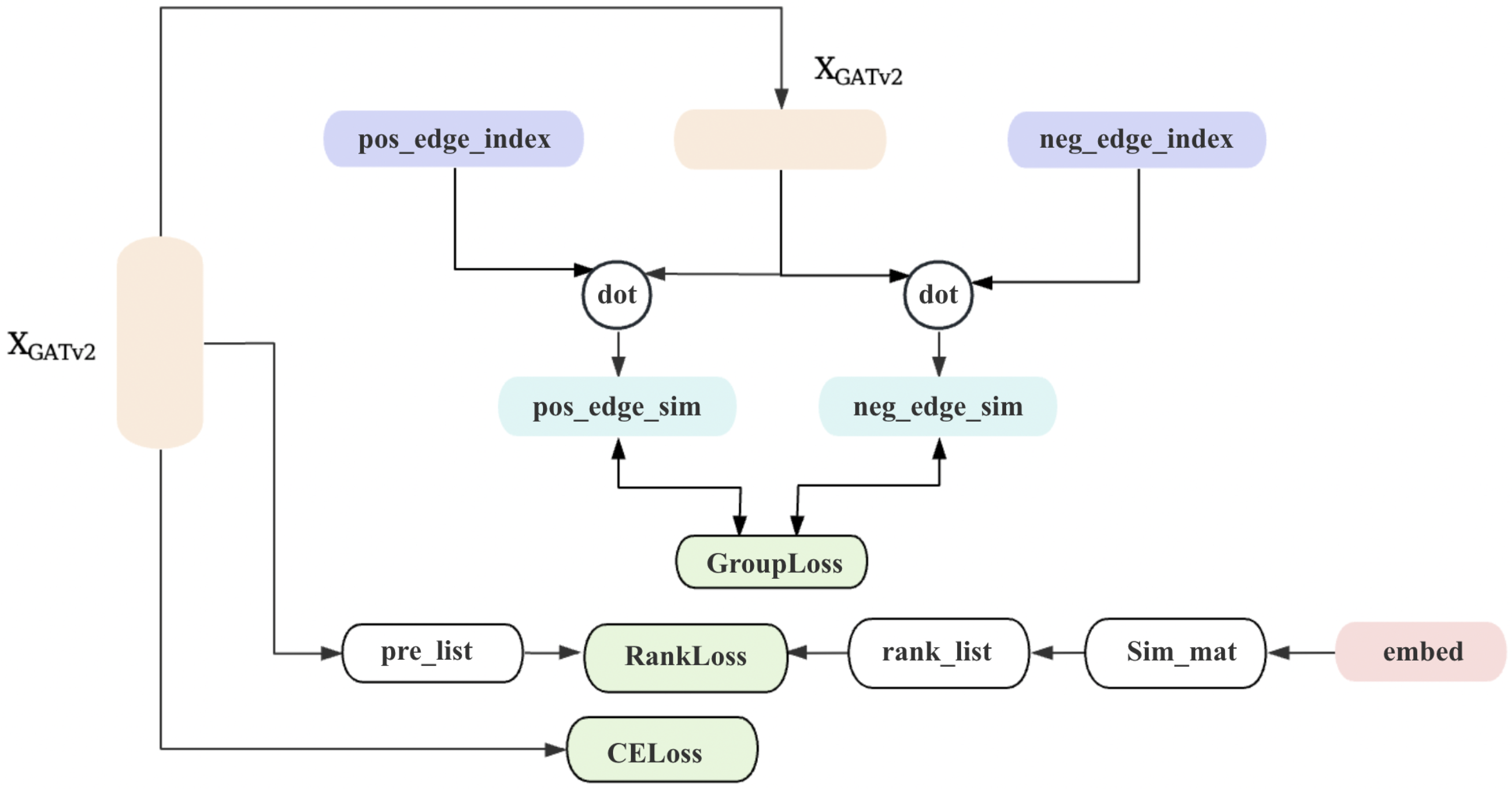
The node feature fusion module uses the local topology information of the nodes to automatically generate fusion coefficients and dynamically update the final node features in heterophilic graphs. LocalSim [36] is utilized to generate fusion coefficients for information integration.

$$\begin{array}{c}\hfill {\Phi }_{\mathrm{i}}={\displaystyle \frac{1}{\left|{\mathrm{N}}_{\mathrm{i}}\right|}}\sum _{{\mathrm{v}}_{\mathrm{j}}\in {\mathrm{N}}_{\mathrm{i}}}{\mathrm{d}}_{\mathrm{ij}}={\displaystyle \frac{1}{\left|{\mathrm{N}}_{\mathrm{i}}\right|}}\sum _{{\mathrm{v}}_{\mathrm{j}}\in {\mathrm{N}}_{\mathrm{i}}}sim\left({\mathrm{x}}_{\mathrm{i}},{\mathrm{x}}_{\mathrm{j}}\right)\end{array}$$

(17)

$$\begin{array}{c}\hfill \left[{\alpha }_{\_}\mathrm{Ao},{\alpha }_{-}\mathrm{L},{\alpha }_{-}\mathrm{H}\right]={MLP}_{\alpha }\left(\left[\Phi ,{\Phi }^2\right]\right)\end{array}$$

(18)

where sim(.,.) is a similarity measure, ${\mathrm{N}}_{\mathrm{i}}$ representing the neighboring nodes of node i. The homophilic node list Ao is fused with ${\tilde{\mathrm{H}}}_{\mathrm{L}}^{\left(\mathrm{k}\right)}$ and ${\tilde{\mathrm{H}}}_{\mathrm{H}}^{\left(\mathrm{k}\right)}$ for learning to obtain the final node representation Z.

$$\begin{array}{c}\hfill {\mathrm{H}}_{\mathrm{Ao}}=Linear\left(\mathrm{MPConv}(\mathrm{Ao},\mathrm{X})\right)\end{array}$$

(19)

$$\begin{array}{c}\hfill {\mathrm{Z}}^{\mathrm{k}}={\alpha }_{\_}{\mathrm{Ao}}^{\mathrm{k}}\odot {\mathrm{H}}_{\mathrm{Ao}}+{\alpha }_{-}{\mathrm{L}}^{\mathrm{k}}\odot {\tilde{\mathrm{H}}}_{\mathrm{L}}^{\left(\mathrm{k}\right)}+{\alpha }_{-}{\mathrm{H}}^{\mathrm{k}}\odot {\tilde{\mathrm{H}}}_{\mathrm{H}}^{\left(\mathrm{k}\right)}\end{array}$$

(20)

where k = 2, …, K, Ao is the list of homophilic nodes obtained from the previous homophilic node extraction module, ⊙ means element-wise product and X represents the node feature matrix.

3.5. Loss Function

To encourage the model to generate distinguishable features for different types of nodes, this paper adopts a feedback optimization [37], as shown in Figure 5, which contains three different loss functions: Grouploss, Rankloss and CEloss.

The positive edge in the graph is represented by two nodes of the same type with an edge connecting them, while the negative edge is represented by two nodes of different types with an edge connecting them. The Grouploss function ${\mathrm{L}}_{\mathrm{grp}}$ samples a certain number of positive edges and negative edges and performs feedback optimization on the model by increasing the similarity between nodes corresponding to positive edges and reducing the similarity between nodes corresponding to negative edges.

$$\begin{array}{cc}\hfill \mathrm{pos}& ={\displaystyle \frac{{\sum }_{(\mathrm{i},\mathrm{j})\in \mathrm{P}}{\mathrm{X}}_{\mathrm{GATv}2}^{\mathrm{T}}\left[{\mathrm{h}}_{\mathrm{i}}\right]·{\mathrm{X}}_{\mathrm{GATv}2}\left[{\mathrm{h}}_{\mathrm{j}}\right]}{\left|\mathrm{P}\right|}}\hfill \end{array}$$

(21)

$$\begin{array}{cc}\hfill {\mathrm{L}}_{\mathrm{pos}}& =-log\left(sig\left(\mathrm{pos}\right)+ϵ\right)\hfill \end{array}$$

(22)

$$\begin{array}{cc}\hfill \mathrm{neg}& ={\displaystyle \frac{{\sum }_{(\mathrm{i},\mathrm{j})\in \mathrm{N}}{\mathrm{X}}_{\mathrm{GATv}}^{\mathrm{T}}\left[{\mathrm{h}}_{\mathrm{i}}\right]·{\mathrm{X}}_{\mathrm{GATv}2}\left[{\mathrm{h}}_{\mathrm{j}}\right]}{\left|\mathrm{N}\right|}}\hfill \end{array}$$

(23)

$$\begin{array}{cc}\hfill {\mathrm{L}}_{\mathrm{neg}}& =-log\left(1-sig\left(\mathrm{neg}+ϵ\right)\right)\hfill \end{array}$$

(24)

$$\begin{array}{c}\hfill {\mathrm{L}}_{\mathrm{grp}}={\mathrm{L}}_{\mathrm{pos}}+{\mathrm{L}}_{\mathrm{neg}}\end{array}$$

(25)

where ${\mathrm{h}}_{\mathrm{i}}$ and ${\mathrm{h}}_{\mathrm{j}}$ represent the feature information of node i and node j, respectively, P is the number of positive class edges sampled, N is the number of negative class edges sampled, sig(.) represents the sigmoid function, $ϵ$ represents small value to mitigate computational errors, and ${\mathrm{X}}_{\mathrm{GATv}2}$ is obtained from the previous feature extraction module.

The Rankloss function ${\mathrm{L}}_{\mathrm{rank}}$ predicts the similarity ranking ${\mathrm{R}}_{\mathrm{i}}$ of a given node’s known sequence based on the cosine similarity between node features, focusing on the ranking relationship between data, which helps to improve the ranking performance of the model.

$$\begin{array}{c}\hfill {\mathrm{R}}_{\mathrm{i}}=\left\{{\mathrm{L}}_{\mathrm{i}}^{\mathrm{intra}}[1:\mathrm{K}]\parallel {\mathrm{L}}_{\mathrm{i}}^{\mathrm{inter}}[-\mathrm{K}:-1]\right\}\end{array}$$

(26)

$$\begin{array}{cc}\hfill {\mathrm{L}}_{\mathrm{i}}^{\mathrm{intra}}& =\left\{{\mathrm{h}}_{\mathrm{j}}^1,\dots ,{\mathrm{h}}_{\mathrm{j}}^{\mathrm{Q}}\mid {\mathrm{Y}}_{{\mathrm{h}}_{\mathrm{j}}^{\mathrm{q}}}={\mathrm{Y}}_{{\mathrm{h}}_{\mathrm{i}}};\right.\hfill \\ \hfill & \left.cos\left({\mathrm{h}}_{\mathrm{i}},{\mathrm{h}}_{\mathrm{j}}^{\mathrm{q}}\right)>cos\left({\mathrm{h}}_{\mathrm{i}},{\mathrm{h}}_{\mathrm{j}}^{\mathrm{q}+1}\right)\right\}\hfill \end{array}$$

(27)

$$\begin{array}{cc}\hfill {\mathrm{L}}_{\mathrm{i}}^{\mathrm{inter}}& =\left\{{\mathrm{h}}_{\mathrm{j}}^1,\dots {\mathrm{h}}_{\mathrm{j}}^{\mathrm{E}}\mid {\mathrm{Y}}_{{\mathrm{h}}_{\mathrm{j}}^{\mathrm{e}}}\ne {\mathrm{Y}}_{{\mathrm{h}}_{\mathrm{i}}};\right.\hfill \\ \hfill & \left.cos\left({\mathrm{h}}_{\mathrm{i}},{\mathrm{h}}_{\mathrm{j}}^{\mathrm{e}}\right)>cos\left({\mathrm{h}}_{\mathrm{i}},{\mathrm{h}}_{\mathrm{j}}^{\mathrm{e}+1}\right)\right\}\hfill \end{array}$$

(28)

where ${\mathrm{h}}_{\mathrm{i}}$ and ${\mathrm{h}}_{\mathrm{j}}$, respectively, represent the feature information of node i and node j, K is a hyperparameter representing the length of the similarity ranking sequence, cos(.,.) represents the cosine similarity function, E represents the count of inter-class nodes for node i, and Q represents the count of intra-class nodes for node i.

The CEloss function ${\mathrm{L}}_{\mathrm{CE}}$ is implemented by reducing the cross-entropy loss between the actual category and the predicted category of the node, ensuring that the model can accurately identify samples of different categories.

$$\begin{array}{c}\hfill {\mathrm{L}}_{\mathrm{CE}}=-\sum _{\mathrm{i}=1}^{\mathrm{N}}{\mathrm{y}}_{{\mathrm{h}}_{\mathrm{i}}}log\left({\mathrm{X}}_{\mathrm{GATv}2}\left[\mathrm{i}\right]\right)\end{array}$$

(29)

where N represents the total number of nodes, ${\mathrm{X}}_{\mathrm{GATv}2}$ represents the predicted class of node i, and ${\mathrm{y}}_{{\mathrm{h}}_{\mathrm{i}}}$ represents the true class of node i.

Therefore, the total loss is given as follows:

$$\begin{array}{c}\hfill \mathrm{L}={\mathrm{L}}_{\mathrm{grp}}+{\mathrm{L}}_{\mathrm{rank}}+{\mathrm{L}}_{\mathrm{CE}}\end{array}$$

(30)

The above elaborate loss function drives the network to preserve critical information.

4. Experiments

In this section, the datasets and details of implementation used in this work are provided in Section 4.1. We give a comparison of experimental results for different models in Section 4.2. Ablative experiments were conducted on the NHSH model and loss function in Section 4.3.

4.1. Experimental Details and Datasets

The experiments are conducted on a Linux server running Ubuntu 22.04.1, using Python 3.10 and PyTorch 2.4.0 for model implementation and testing. The system provides an efficient environment for training and evaluating the model.

In this study, we choose eight public datasets to validate the model, including five homophilic datasets: Cora, Citeseer, PubMed, Computer, and Photo, and three heterophilic datasets: Chameleon, Squirrel, and Actor. The dataset details are provided in

Table 2. Homophily and Heterophily Dataset.

	Homophily					Heterophily
	Cora	Citeseer	PubMed	Computer	Photo	Chameleon	Squirrel	Actor
Classes	7	6	5	10	8	5	5	5
Features	1433	3703	500	767	745	2325	2089	932
Nodes	2708	3327	19,717	13,752	7650	2277	5201	7600
Edges	5278	4552	44,324	491,722	238,162	31,371	198,353	26,659

. We randomly split the node set of a dataset according to the ratio 60%/20%/20% for training, validation and test set, respectively.

During the training phase, for the homophilic Node Extraction Module, the hyperparameters are set as follows: the learning rate is selected from 0.01, 0.001, 0.005, and the weight decay is chosen from 5 $\times {10}^{-4}$, 5 $\times {10}^{-5}$. For the Homophilic Node Extraction Module, the layer setting k for Cora, Citeseer, PubMed, Computer, Photo, Chameleon, Squirrel, and Actor datasets, respectively, are 6, 11, 11, 6, 14, 22, 16, and 21. Hidden channels are chosen from 16, 32, 64. Dropout is adjusted within the range of 0.4 to 0.9.

For evaluation metrics, we adopt graph homophily as the evaluation metric for the homophilic node extraction module. For the node classification task, we adopt node classification accuracy as the metric. We compare our model with eight state-of-the-art methods, including MLP [38], GCN [2], GAT [25], APPNP [27], GPR-GNN [22], JKNET [39], GOAL [40] and LSGNN [36], and conduct experiments strictly following the settings provided in their original papers and use the pretrained models provided by the authors.

4.2. Comparison with State-of-the-Art Methods

As can be seen from

Table 3. Overall performance of graph classification on eight datasets measured by classification accuracy.

	Cora	Citeseer	PubMed	Computer	Photo	Chameleon	Squirrel	Actor
MLP	72.09	71.67	87.47	83.59	90.49	46.55	30.67	28.75
GCN	87.50	75.11	87.20	83.55	89.30	62.72	47.26	29.98
GAT	88.25	75.75	85.88	85.36	90.81	62.19	51.80	28.17
APPNP	88.36	76.03	86.21	88.32	94.44	50.88	33.58	29.82
GPR-GNN	88.65	75.70	88.53	87.63	94.60	67.96	49.52	30.78
JKNET	86.99	75.38	88.64	86.97	92.68	64.63	44.91	28.48
GOAL	88.75	77.15	89.25	91.33	95.60	71.65	60.53	36.46
LSGNN	88.49	76.71	90.23	90.45	95.02	79.04	72.81	36.18
Running Times(s)	0.24	0.50	2.16	1.17	0.73	0.39	1.31	1.48
NHSH	90.69	83.20	90.70	91.99	96.46	86.81	83.18	39.65

The best result is highlighted in bold, and the second-best is italicized and underlined.

, the proposed NHSH has the highest accuracy on all datasets. For the Cora, Citeseer, Computer, and Photo, NHSH outperforms GOAL by 1.94%, 6.05%, 0.66%, and 0.86%, respectively. Since GOAL reconstructs the homophilic graph based on the original graph, it uses a fixed coefficient to merge the node feature information in the reconstructed graph, which may destroy the original homophily of the graph. In contrast, NHSH can not only use filters to extract spectral information without destroying the original graph structure but also strengthen node features through homophilic information. Additionally, it leverages the local topological information of nodes to automatically generate fusion coefficients and dynamically update the fusion parameters. On the PubMed dataset, NHSH is 0.47% higher than LSGNN. LSGNN uses both high-frequency and low-frequency filters to learn spectral information of nodes, but on a large-scale dataset like PubMed, fusing node homophilic information can better extract the features of nodes of the same type.

For the heterophilic graph datasets, the accuracy of all models decreased to varying degrees, reflecting the challenging nature of heterophilic graphs for graph neural networks. Nevertheless, NHSH demonstrates superior performance, achieving 7.77% and 10.37% higher accuracy than LSGNN on the Chameleon and Squirrel datasets, respectively. This improvement is attributed to NHSH’s ability to integrate homophilic node information, which is neglected by LSGNN. Relying solely on high-frequency and low-frequency information is insufficient to capture comprehensive node features, especially in heterophilic graphs where node relationships are more complex. On the Actor dataset, the accuracy of NHSH is 3.19% higher than GOAL. Since the node feature dimensions of Actor are less than those of Chameleon and Squirrel, NHSH provides richer information for learning node features by fusing homophilic node information, enabling the model to better understand the relationships and features between nodes, therefore improving the accuracy of node classification.

4.3. Ablation Studies

The ablation study presented in this paper systematically evaluates the effectiveness of the proposed model by isolating and analyzing the contributions of its individual components and configurations. It comprises five key experiments: (1) analysis of the homophilic node extraction, (2) analysis of the heterophilic spectrum extraction, (3) analysis of the node feature fusion, (4) analysis of the loss function, and (5) analysis of the hyperparameters.

The structured approach adopted in the ablation study validates the proposed model by thoroughly assessing the impact of each component, ensuring a comprehensive and reliable evaluation. The findings not only underscore the strengths of the proposed methodology but also offer valuable insights for the design and optimization of graph-based models across diverse applications.

4.3.1. Analysis of the Homophilic Node Extraction

In order to verify the effectiveness of homophilic node extraction, six different model variants are set: Linear + GCN, GCN + GCN, Linear + GAT, Linear + GATv2, GCN + GAT and GCN + GATv2. The experiments use the same parameter settings and the homophily ratio of the generated graphs as the evaluation metric.

First, we conduct comparative experiments on Linear and GCN. The experimental results show that the GCN-based extraction module performs better in local structure embedding mining. This is mainly due to the fact that GCN can effectively capture and utilize the topological structure information of the graph to represent the relationship between nodes.

Then, we conduct comparative experiments on Linear + GAT and GCN + GAT. Experimental results further show that using the attention mechanism can focus on the link relationship between nodes and their neighbors and extract the local structural features of nodes in a more fine-grained manner.

Furthermore, we compared the feature extraction capabilities of GAT and GATv2 based on the GCN module. Experimental results show that the reconstructed graphs using nodes extracted by GATv2 are superior to GAT in terms of homophily. This is because GATv2 can better handle the complex relationships between nodes and generate more discriminative node embedding representations. As can be seen from

Table 4. Homophilic node extraction ablation studies.

Local Structure Embedded	Feature Extraction	Cora	Citeseer	Chameleon	Squirrel	Actor	Photo	Computers	PubMed
Linear	GCN	0.8416	0.7341	0.7461	0.6102	0.2114	0.9207	0.8100	0.7779
GCN	GCN	0.8663	0.7915	0.7721	0.6680	0.2439	0.9273	0.8448	0.8544
Linear	GAT	0.7920	0.7396	0.7718	0.6036	0.2259	0.9188	0.8383	0.7668
Linear	GATv2	0.8309	0.7420	0.7882	0.6296	0.2145	0.9268	0.8345	0.7722
GCN	GAT	0.8779	0.7928	0.8017	0.7208	0.2504	0.9339	0.8743	0.8590
GCN	GATv2	0.9055	0.8230	0.8169	0.7282	0.3098	0.9438	0.8764	0.8848

The best result is highlighted in bold, and the second-best is italicized and underlined.

, the performance of GCN + GATv2 is consistently better than other configurations. Therefore, this paper selects GCN + GATv2 as the model configuration of the homophilic node extraction.

In order to verify whether the homophilic node extraction module can effectively extract homophilic nodes, we visualized the extracted node structure in heterophilic and homophilic datasets, as shown in Figure 6. The figure shows that the nodes extracted by the homophilic node extraction module are more likely to be connected to the same type of nodes.

4.3.2. Analysis of the Heterophilic Spectrum Extraction

To verify the effectiveness of heterophilic spectrum extraction, three different model variants are set: using only high-frequency filters, only low-frequency filters, and a combination of both filters. The experiments use the same parameter settings and use the accuracy of node classification as the evaluation metric.

First, only low-pass filters are used to extract global features of nodes, which has good results on homophilic graphs. From the experimental results in

Table 5. High-pass and low-pass filter ablation studies.

	Cora	Citeseer	Chameleon	Squirrel	Actor	Photo	Computers	PubMed
${\mathrm{F}}_{\mathrm{high}}$	79.48	71.68	78.44	73.16	37.87	92.81	88.59	89.71
${\mathrm{F}}_{\mathrm{low}}$	87.58	76.62	73.90	64.32	37.91	93.43	91.77	89.87
${\mathrm{F}}_{\mathrm{low}}$ + ${\mathrm{F}}_{\mathrm{high}}$	89.20	78.85	76.31	73.64	38.26	95.36	91.85	90.31

The best result is highlighted in bold, and the second-best is italicized and underlined.

, it is obvious that the node classification accuracy of only low-pass filters on homophilic graph datasets (such as Cora and Citeseer) is significantly higher than that of heterophilic graph datasets (such as Chameleon and Squirrel). This is because nodes of the same category in homophilic graphs tend to be linked together, and low-pass filters can effectively capture this feature and generate representative features. However, relying solely on low-frequency information may ignore the subtle differences and dynamic changes between different node types in heterophilic graphs.

Second, only high-pass filters are used to extract node feature information. High-pass filters can sensitively capture rapid changes in node features and usually perform well on heterogeneous graphs. As shown in Table 3, the use of the high-pass filter model on heterophilic graph datasets (such as Chameleon and Squirrel) improves the accuracy by 4.54% and 8.84%, respectively, compared to the low-pass filter model. However, models that rely solely on high-frequency information are susceptible to noise interference, which affects their generalization ability.

Finally, a combination of high-pass and low-pass filters is used to extract high-frequency and low-frequency information in the heterophilic graph, aiming to construct a more comprehensive and accurate node feature representation. As shown in Table 3, the model integrating high-pass and low-pass filters achieves the best performance on both homophilic and heterophilic graph datasets.

It is worth noting that on the Chameleon dataset, the node classification accuracy of the model using only the high-pass filter is even better than that of the combination of the high-pass filter and the low-pass filter. This is mainly attributed to the specific properties of the nodes in the Chameleon dataset, which makes high-frequency information particularly important. However, in order to maintain the generalization ability of the model, we still choose the combined filter to extract node features in this paper.

4.3.3. Analysis of the Node Feature Fusion

In order to verify the effectiveness of node feature fusion, we specifically compare two variants: a model that only uses spectral information (${\mathrm{NHSH}}_{\mathrm{no}\_\mathrm{homo}}$) and a model that uses fused feature (NHSH). The experimental results in

Table 6. Analyses about the node feature fusion.

	Cora	Citeseer	Chameleon	Squirrel	Actor	Photo	Computers	PubMed
${\mathrm{NHSH}}_{\mathrm{no}\_\mathrm{homo}}$	87.79 ± 1.41	76.95 ± 1.90	75.11 ± 1.20	71.59 ± 2.05	37.17 ± 1.09	95.36 ± 0.77	91.34 ± 0.51	89.84 ± 0.47
NHSH	89.46 ± 1.23	82.09 ± 1.11	85.81 ± 1.00	82.40 ± 0.78	39.05 ± 0.60	95.89 ± 0.57	91.46 ± 0.53	90.13 ± 0.57

The best result is highlighted in bold.

show that the node classification accuracy of the NHSH model is better than the former on all graph datasets, especially on heterophilic graphs, where the accuracy is improved by nearly 10%. The results show that incorporating homophilic node information into spectral information can effectively enhance the representation ability of nodes and the generalization ability of the model. NHSH can better capture the local structure and similarity between nodes, enabling the model to more accurately handle noise and local changes in graph data.

We also visualized the feature information of fused information, homophilic node information, high-frequency information, and low-frequency information in the form of a heat map, as shown in Figure 7. We compared the feature information after the first epoch of the model with the feature information after the last epoch and can intuitively feel the changes in node feature information after learning.

In order to have a more intuitive display of feature information enhancement, we visualize the intermediate process of feature extraction in the form of a scatter plot, as shown in Figure 8. As the model is continuously iteratively optimized, the feature information of nodes in the same category gradually aggregates, and finally, the node classification is achieved.

4.3.4. Analysis of the Loss Function

In order to verify the effectiveness of the loss function, We explore the necessity of three different loss functions (loss_group, loss_rank, and loss_ce) in training optimization. The experiments use the same parameter settings and the homophily of the graph as the evaluation metric.

We conducted a total of 7 experiments covering various combinations of loss modules, with the following experimental settings: only using a single loss (i.e., loss_rank, loss_group, and loss_ce) to verify the individual effect; using a combination of two loss (i.e., loss_group + loss_ce, loss_rank + loss_ce, and loss_rank + loss_group); and using all three loss at the same time (loss_rank + loss_group + loss_ce).

As can be seen from

Table 7. Feedback optimization module ablation studies. We conducted a total of seven experiments covering various combinations of loss modules, and we utilized generated node homophily as the evaluation metric. Here, ✓ denotes the presence of the component, while × signifies its absence.

loss_rank	loss_group	loss_ce	Cora	Citeseer	Chameleon	Squirrel	Actor	Photo	Computers	PubMed
✓	×	×	0.2661	0.4200	0.2294	0.2794	0.2515	0.2769	0.2631	0.4049
×	✓	×	0.8445	0.8183	0.7258	0.7057	0.3016	0.9191	0.7548	0.8791
×	×	✓	0.2930	0.2106	0.3142	0.2219	0.2258	0.2780	0.3125	0.3453
×	✓	✓	0.9137	0.8070	0.7552	0.7162	0.2800	0.9366	0.8543	0.8769
✓	×	✓	0.4781	0.3571	0.6848	0.2248	0.2029	0.8405	0.6540	0.8227
✓	✓	×	0.8905	0.8222	0.7408	0.6817	0.2806	0.9443	0.8170	0.8632
✓	✓	✓	0.9055	0.8230	0.8169	0.7282	0.3098	0.9438	0.8764	0.8848

The best result is highlighted in bold, and the second-best is italicized and underlined.

, The model that uses three losses simultaneously achieves the best performance on all datasets, fully demonstrating the indispensability of the loss in model training. Specifically, loss_group helps capture the group information in the graph data, therefore improving the generalization ability of the model; loss_rank focuses on the ranking relationship between the data, which helps to improve the ranking performance of the model; loss_ce is responsible for optimizing the classification performance of the model to ensure that the model can accurately identify samples of different categories.

We observed that the loss_group loss function has the most significant impact on improving model performance. On the Cora dataset, our model achieved node homogeneity of 84.45%, and on the Squirrel data set, the node homogeneity reached 70.57%. The above results show that obtaining node group information can help improve model performance, whether it is a homophilic graph or a heterophilic graph. In addition, when using two losses, on the Cora, Citeseer, and Squirrel datasets, the homophily of the models with loss_group + loss_ce and loss_rank + loss_group is more than 40% higher than that of the model with loss_rank + loss_ce, which further highlights the importance of the loss_group module and the impact of node homophily on model performance.

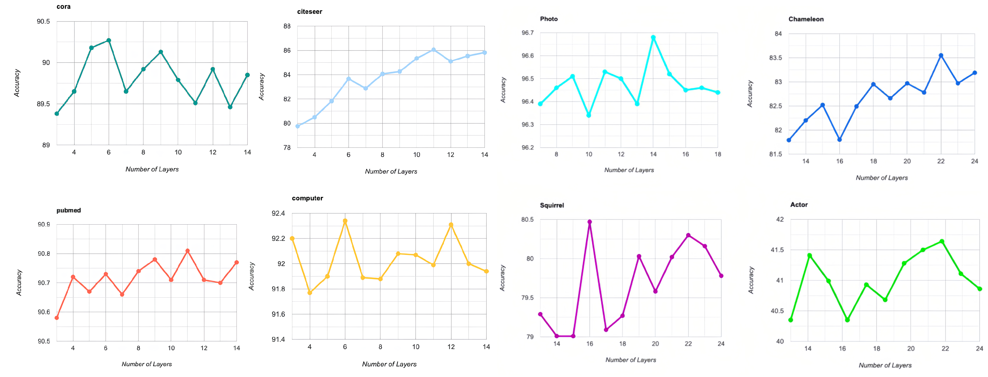
4.3.5. Analysis of the Hyperparameters

In this experiment, we delved into the relationship between model performance and the number of convolutional layers in the model. During the experiment, the number of convolutional layers K was gradually increased, and the step size was adjusted to 1 each time. The experimental results are shown in Figure 9.

The experimental visualization results show that for homogeneous datasets, the optimal value is usually smaller. In addition, when the number of categories of nodes in the graph is less than or equal to 6, the accuracy of the model is positively correlated with the number of layers K. For datasets with more than 6 node categories in the graph, the accuracy of the model fluctuates greatly as the number of layers K increases. Therefore, this paper finally determines the optimal settings of the number of layers K for Cora, Citeseer, PubMed, Photo, Computer, Chameleon, Squirrel, and Actor datasets as 6, 11, 11, 6, 14, 22, 16, and 21, respectively.

5. Conclusions

In this paper, we propose a novel graph hybrid-learning framework based on Node Homophily and Spectral Heterophily (NHSH), which can extract homophilic node information and fuse high-frequency and low-frequency information of the graph. Compared with many GNNs that only consider the spectral information or homophilic node information of the graph, the proposed NHSH has better performance for both homophilic and heterophilic graph data. The homophilic node extraction module we proposed can better extract and utilize the homophily of nodes, providing richer and more effective node features for subsequent spectrum information fusion. In addition, we use LocalSim to learn the fusion coefficient to achieve feature fusion, avoiding the tedious process of manual adjustment. Extensive evaluations over eight benchmark datasets show that our proposed method can offer comparable or superior state-of-the-art performance on both homophilic and heterophilic graphs. Therefore, NHSH provides new ideas for graph data analysis.

Although NHSH works well on the graphs used in this study, further work is needed to evaluate its performance on large-scale graphs. Future studies could focus on optimizing the computational efficiency of the method to handle graphs with millions of nodes and edges.

References

1. Pan, C.H.; Qu, Y.; Yao, Y.; Wang, M.J.S. HybridGNN: A Self-Supervised Graph Neural Network for Efficient Maximum Matching in Bipartite Graphs. Symmetry 2024, 16, 1631. [Google Scholar] [CrossRef]
2. Kipf, T.N.; Welling, M. Semi-supervised classification with graph convolutional networks. arXiv 2016, arXiv:1609.02907. [Google Scholar]
3. Wu, L.; Lin, H.; Liu, Z.; Liu, Z.; Huang, Y.; Li, S.Z. Homophily-enhanced self-supervision for graph structure learning: Insights and directions. IEEE Trans. Neural Netw. Learn. Syst. 2023, 35, 12358–12372. [Google Scholar] [CrossRef]
4. Khoushehgir, F.; Noshad, Z.; Noshad, M.; Sulaimany, S. NPI-WGNN: A Weighted Graph Neural Network Leveraging Centrality Measures and High-Order Common Neighbor Similarity for Accurate ncRNA–Protein Interaction Prediction. Analytics 2024, 3, 476–492. [Google Scholar] [CrossRef]
5. Hamilton, W.; Ying, Z.; Leskovec, J. Inductive representation learning on large graphs. Adv. Neural Inf. Process. Syst. 2017, 30. [Google Scholar]
6. Wang, Y.; Xiang, S.; Pan, C. Improving the Homophily of Heterophilic Graphs for Semi-Supervised Node Classification. In Proceedings of the 2023 IEEE International Conference on Multimedia and Expo (ICME), Brisbane, Australia, 10–14 July 2023. [Google Scholar]
7. Li, J.; Zheng, R.; Feng, H.; Li, M.; Zhuang, X. Permutation equivariant graph framelets for Heterophilous graph learning. IEEE Trans. Neural Netw. Learn. Syst. 2024, 35, 11634–11648. [Google Scholar] [CrossRef]
8. Chen, R. Preserving Global Information for Graph Clustering with Masked Autoencoders. Mathematics 2024, 12, 1574. [Google Scholar] [CrossRef]
9. Huang, W.; Guan, X.; Liu, D. Revisiting homophily ratio: A relation-aware Graph Neural Network for homophily and heterophily. Electronics 2023, 12, 1017. [Google Scholar] [CrossRef]
10. Oishi, Y.; Kaneiwa, K. Multi-Duplicated Characterization Of Graph Structures Using Information Gain Ratio For Graph Neural Networks. IEEE Access 2023, 11, 34421–34430. [Google Scholar] [CrossRef]
11. Park, H.S.; Park, H.M. Enhancing Heterophilic Graph Neural Network Performance Through Label Propagation in K-Nearest Neighbor Graphs. In Proceedings of the 2024 IEEE International Conference on Big Data and Smart Computing (BigComp), Bangkok, Thailand, 18–21 February 2024. [Google Scholar]
12. Guan, X.; Wang, D.; Xiong, C.; Li, S.; Chen, Y. PBGAN: Path Based Graph Attention Network for Heterophily. In Proceedings of the 2022 26th International Conference on Pattern Recognition (ICPR), Montreal, QC, Canada, 21–25 August 2022. [Google Scholar]
13. Sun, J.; Zhang, L.; Zhao, S.; Yang, Y. Improving your graph neural networks: A high-frequency booster. In Proceedings of the 2022 IEEE International Conference on Data Mining Workshops (ICDMW), Orlando, FL, USA, 28 November–1 December 2022. [Google Scholar]
14. Wang, Y.; Hu, L.; Cao, X.; Chang, Y.; Tsang, I.W. Enhancing Locally Adaptive Smoothing of Graph Neural Networks Via Laplacian Node Disagreement. IEEE Trans. Knowl. Data Eng. 2023, 36, 1099–1112. [Google Scholar] [CrossRef]
15. Gu, M.; Yang, G.; Zhou, S.; Ma, N.; Chen, J.; Tan, Q.; Bu, J. Homophily-enhanced structure learning for graph clustering. In Proceedings of the 32nd ACM International Conference on Information and Knowledge Management, Birmingham, UK, 21–25 October 2023. [Google Scholar]
16. Bruna, J.; Zaremba, W.; Szlam, A.; LeCun, Y. Spectral networks and locally connected networks on graphs. arXiv 2013, arXiv:1312.6203. [Google Scholar]
17. Wu, F.; Souza, A.; Zhang, T.; Fifty, C.; Yu, T.; Weinberger, K. Simplifying graph convolutional networks. In Proceedings of the International Conference on Machine Learning, PMLR, Long Beach, CA, USA, 9–15 June 2019. [Google Scholar]
18. Lingam, V.; Ragesh, R.; Iyer, A.; Sellamanickam, S. Simple truncated svd based model for node classification on heterophilic graphs. arXiv 2021, arXiv:2106.12807. [Google Scholar]
19. Xu, B.; Shen, H.; Cao, Q.; Cen, K.; Cheng, X. Graph convolutional networks using heat kernel for semi-supervised learning. arXiv 2020, arXiv:2007.16002. [Google Scholar]
20. Wang, X.; Zhang, M. How powerful are spectral graph neural networks. In Proceedings of the International Conference on Machine Learning, PMLR, Baltimore, MD, USA, 17–23 July 2022. [Google Scholar]
21. He, M.; Wei, Z.; Xu, H. Bernnet: Learning arbitrary graph spectral filters via bernstein approximation. Adv. Neural Inf. Process. Syst. 2021, 34, 14239–14251. [Google Scholar]
22. Chien, E.; Peng, J.; Li, P.; Milenkovic, O. Adaptive universal generalized pagerank graph neural network. arXiv 2020, arXiv:2006.07988. [Google Scholar]
23. Awasthi, A.K.; Garov, A.K.; Sharma, M.; Sinha, M. GNN model based on node classification forecasting in social network. In Proceedings of the 2023 International Conference on Artificial Intelligence and Smart Communication (AISC), Greater Noida, India, 27–29 January 2023. [Google Scholar]
24. Shetty, R.D.; Bhattacharjee, S.; Thanmai, K. Node Classification in Weighted Complex Networks Using Neighborhood Feature Similarity. IEEE Trans. Emerg. Top. Comput. Intell. 2024, 8, 3982–3994. [Google Scholar] [CrossRef]
25. Veličković, P.; Cucurull, G.; Casanova, A.; Romero, A.; Lio, P.; Bengio, Y. Graph attention networks. arXiv 2017, arXiv:1710.10903. [Google Scholar]
26. Pan, J.; Lin, H.; Dong, Y.; Wang, Y.; Ji, Y. MAMF-GCN: Multi-scale adaptive multi-channel fusion deep graph convolutional network for predicting mental disorder. Comput. Biol. Med. 2022, 148, 105823. [Google Scholar] [CrossRef] [PubMed]
27. Gasteiger, J.; Bojchevski, A.; Günnemann, S. Predict then propagate: Graph neural networks meet personalized pagerank. arXiv 2018, arXiv:1810.05997. [Google Scholar]
28. Pei, H.; Wei, B.; Chang, K.C.C.; Lei, Y.; Yang, B. Geom-gcn: Geometric graph convolutional networks. arXiv 2020, arXiv:2002.05287. [Google Scholar]
29. Abu-El-Haija, S.; Perozzi, B.; Kapoor, A.; Alipourfard, N.; Lerman, K.; Harutyunyan, H.; Galstyan, A. Mixhop: Higher-order graph convolutional architectures via sparsified neighborhood mixing. In Proceedings of the international Conference on Machine Learning, PMLR, Long Beach, CA, USA, 9–15 June 2019. [Google Scholar]
30. Roy, K.K.; Roy, A.; Rahman, A.M.; Amin, M.A.; Ali, A.A. Node embedding using mutual information and self-supervision based bi-level aggregation. In Proceedings of the 2021 International Joint Conference on Neural Networks (IJCNN), Shenzhen, China, 18–22 July 2021. [Google Scholar]
31. Zhu, J.; Rossi, R.A.; Rao, A.; Mai, T.; Lipka, N.; Ahmed, N.K.; Koutra, D. Graph neural networks with heterophily. Proc. Aaai Conf. Artif. Intell. 2021, 35, 11168–11176. [Google Scholar] [CrossRef]
32. Ma, Y.; Liu, X.; Shah, N.; Tang, J. Is homophily a necessity for graph neural networks? arXiv 2021, arXiv:2106.06134. [Google Scholar]
33. Chen, D.; Lin, Y.; Li, W.; Li, P.; Zhou, J.; Sun, X. Measuring and relieving the over-smoothing problem for graph neural networks from the topological view. Proc. Aaai Conf. Artif. Intell. 2020, 34, 3438–3445. [Google Scholar] [CrossRef]
34. Bo, D.; Wang, X.; Shi, C.; Shen, H. Beyond low-frequency information in graph convolutional networks. Proc. Aaai Conf. Artif. Intell. 2021, 35, 3950–3957. [Google Scholar] [CrossRef]
35. Brody, S.; Alon, U.; Yahav, E. How attentive are graph attention networks? arXiv 2021, arXiv:2105.14491. [Google Scholar]
36. Chen, Y.; Luo, Y.; Tang, J.; Yang, L.; Qiu, S.; Wang, C.; Cao, X. LSGNN: Towards general graph neural network in node classification by local similarity. arXiv 2023, arXiv:2305.04225. [Google Scholar]
37. Zheng, X.; Zhang, M.; Chen, C.; Zhang, Q.; Zhou, C.; Pan, S. Auto-heg: Automated graph neural network on heterophilic graphs. In Proceedings of the ACM Web Conference 2023, Austin, TX, USA, 30 April–4 May 2023. [Google Scholar]
38. Taud, H.; Mas, J.F. Multilayer perceptron (MLP). In Geomatic Approaches for Modeling Land Change Scenarios; Springer: Cham, Switzerland, 2018; pp. 451–455. [Google Scholar]
39. Chen, M.; Wei, Z.; Huang, Z.; Ding, B.; Li, Y. Simple and deep graph convolutional networks. In Proceedings of the International Conference on Machine Learning, PMLR, Virtual, 13–18 July 2020. [Google Scholar]
40. Zheng, Y.; Zhang, H.; Lee, V.; Zheng, Y.; Wang, X.; Pan, S. Finding the missing-half: Graph complementary learning for homophily-prone and heterophily-prone graphs. In Proceedings of the International Conference on Machine Learning, PMLR, Honolulu, HI, USA, 23–29 July 2023. [Google Scholar]
Figure 1. Visualization of homophily graph and heterophily graph. (a,b) are homophilic graph, (c,d) are heterophilic graph. Edges represent nodes connected to each other.
Symmetry 17 00115 g001
Figure 2. Overview of the NHSH architecture.
Symmetry 17 00115 g002
Figure 3. Illustration of node local structure embedding module.
Symmetry 17 00115 g003
Figure 4. Illustration of feature extraction module. It is mainly implemented by the dynamic attention mechanism GATv2.
Symmetry 17 00115 g004
Figure 5. Illustration of Feedback optimization module. It is mainly implemented by three different loss functions: the Grouploss, Rankloss, and CEloss.
Symmetry 17 00115 g005
Figure 6. We visualize the structure of the extracted node from the homophilic node extraction module on cora, citeseer, squirrel, and chameleon, and the image show clusters of 7, 6, 5, and 5, respectively, corresponding to the node classes.
Symmetry 17 00115 g006
Figure 7. Visualization of feature information in the form of heat maps. (a,b) are hybrid-learning information heat maps. (c,d) are homophilic node information heat maps. (e,f) are high-frequency information heat maps. (g,h) are low-frequency information heat maps. Furthermore, where (a,c,e,g) are the feature information heat maps obtained after the first epoch, (b,d,f,h) are the feature information heat maps obtained after the last epoch.
Symmetry 17 00115 g007
Figure 8. Visualization of intermediate feature information in the form of scatters for citeseer and squirrel. In order to obtain a more intuitive feel for the enhancement of feature information by our model, we visualize the feature information obtained through different numbers of epochs and present it in the form of a scatter plot.
Symmetry 17 00115 g008
Figure 9. Accuracy of different number of training layers K on eight datasets. During the experiment, we gradually increased the number of training layers K and adjusted the step size to 1 each time. We present it in the form of a line graph.
Symmetry 17 00115 g009