1. Introduction
The goal of computerized tomography [
1] is the three-dimensional reconstruction of generic objects slice by slice. For a physical medium, a variable proportional to the density is summed along a sequence of rays to form a projection. The application of choice is medical diagnostics, and several hundreds of projections are needed because the body consists of numerous organs with different absorption rates. In the particular case of objects with a few density values, it is possible to reduce the number of projections, thus defining the so-called discrete tomography [
2].
Classical algorithms of computerized tomography have been unable to provide satisfying results in the case of discrete tomography [
3]. Although in the literature there are many works from a theoretical point of view, this latter reconstruction task is still particularly hard to face. Moreover, all current studies involve reconstructing a single slice at a time, without actually considering the entire three-dimensional object. The computational complexity of three-dimensional discrete tomography with missing data has been considered in [
4] again from a mere theoretical viewpoint.
It can be proved in polynomial time whether there exists any object compatible with just a pair of projections [
5,
6]; the complexity of this reconstruction process becomes NP-hard in the case of at least three projections along non-parallel directions [
7,
8]. In addition, the number of binary images compatible with a small set of projections is typically huge even if these images can be very different from each other [
9].
Exact reconstruction requires additional information: not only a big enough number of projections, but also the geometric and topological properties of the object [
10]. For example, in crystallography, we may need some knowledge about the types of atoms to analyze, the probability to find holes inside the object and its topology (e.g., some configurations are energetically unstable) [
11,
12]. Particular two-dimensional reconstruction algorithms were designed for ad hoc classes of binary images (e.g., periodic images, which have repetitions of pixels along some directions [
13]; hv-convex polyominoes, which are connected sets with 4-connected rows and columns [
14,
15], convex objects [
16]; and symmetric convex polygons [
17], which is different from respecting the symmetry of particular organs of the patient [
18]). Networks flows and Boolean solvers have been proposed to reduce the number of potential solutions [
19]. Recently, a method has been proposed to determine the suitable directions of projections in the case of two-dimensional convex models [
20]. Even a relatively seemingly simple case such as two-dimensional orthogonal discrete tomography with a Hamiltonicity constraint was proven to be NP-complete [
21].
Heuristic approaches [
22,
23,
24,
25] have been applied to the reconstruction problem whereas evolutionary methodologies have shown their feasibility to reconstruct specific kinds of images such as circular or elliptical objects [
26,
27], images from interferometric fringes [
28,
29] and compact binary images [
30]. A combined tabu-search and algebraic reconstruction algorithm has been developed for discrete tomography, although it needs a large number of projections [
31].
Two-dimensional discrete tomography can be extended to the three-dimensional case by assuming some similarity between pairs of adjacent slices. This corresponds to the introduction of a model of the object to reconstruct, which may be useful from a general point of view though unfeasible in the case of security and medical imaging. To the best of our knowledge, no real, meaningful approach has been proposed so far.
This paper is organized as follows. After the description of the main parts of our evolutionary algorithm (
Section 2), we describe the used dataset and the results (
Section 3). Conclusions will highlight the advantages of the adopted technique, providing inspiration for future developments (
Section 4).
2. Materials and Methods
In short, in a genetic algorithm, candidate solutions, called individuals, evolve from one generation to another toward better and better solutions: individuals can mate to exchange information and can suffer alterations in the hope that their new genetic arrangement is better. Obviously, the solution is not known, but it is known what it will have to look like.
Indeed, a fitness function evaluates how much each individual approaches the unknown solution and lets only the best individuals survive in the next generation according to an evolutionary pressure: the best individual of the entire process is presented as the final solution. To cover as large an area of the search space as possible, various techniques are considered to prevent individuals from being overly similar to each other. A description of modern evolutionary strategies is given in [
32].
It should be noted that we do not know the exact solution to the problem, but a different representation of its appearance—specifically, its projections. Therefore, our goal is finding a data volume that satisfies the same set of projections, assuming that this is the desired solution. In fact, there is no guarantee that the output of any evolutionary algorithm will actually be the desired solution, even if it satisfies the entire set of projections. As a rule of thumb, the greater the amount of input information (i.e., the number of projections), the greater the chance that the solution will be correct.
This paper presents a substantially revised and extended account of research previously reported in [
30]. Compared to that work, we are now able to directly reconstruct three-dimensional objects from a reduced number of appropriate projections in a reasonable time (please see
Section 3). We set aside the initial idea of assuming that there is a correlation between adjacent slices because this implicitly introduces a model of the volume to reconstruct. Instead, our new approach forces the reconstruction by oblique projections that intersect different areas of separate slices. Therefore, our approach avoids the introduction of any model that could force the reconstruction of the object towards a user-defined, albeit incorrect, shape.
The algorithm keeps the population size constant during the evolution, and it stops when a suitable solution is found. This avoids a rapid performance degradation. In any case, a halt condition is established by the total number of allowed generations.
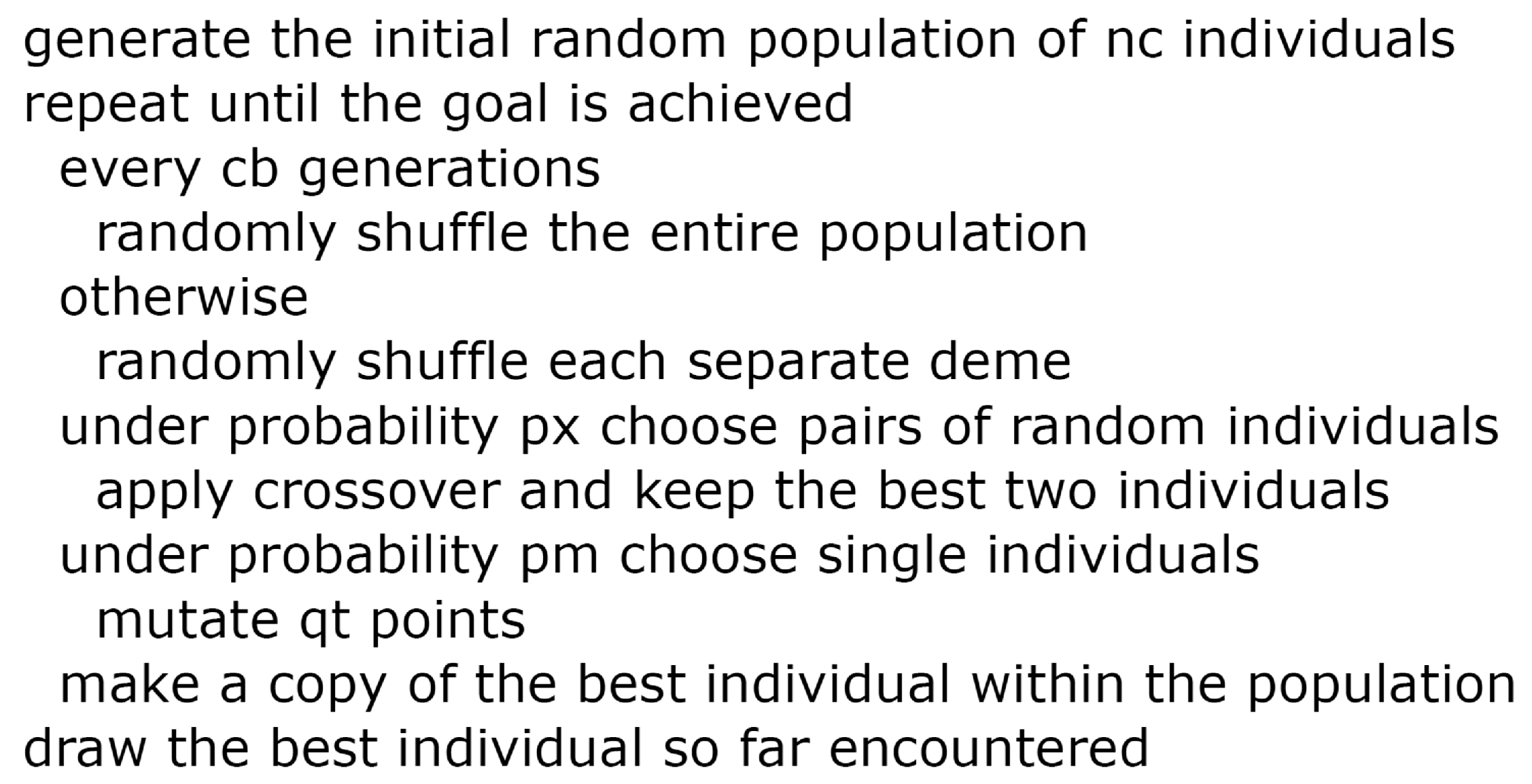
A minimalist representation of the proposed algorithm is shown in
Figure 1 (details will be provided shortly). The most suitable cardinality
of the population, number
of generations, and probabilities
and
for the genetic operators will be considered in
Section 3. For the sake of clarity, from now on, we will use the term
random to indicate a pseudorandom generation according to a uniform probability distribution. In particular, we used the Mersenne Twister [
33] algorithm with seed initialized according to the current time before each reconstruction to exclude repetitions in the experiments.
2.1. Individuals
The proposed methodology allows us to directly reconstruct cubes with binary values; for practical purposes, we will consider points with and 128. It must be noted that these sizes correspond to binary images with about , and pixels, respectively, in the case of the standard two-dimensional discrete tomography; this provides a rough sense to compare our methodology against those already known in the literature in terms of data complexity.
We define an individual as a binary matrix of size
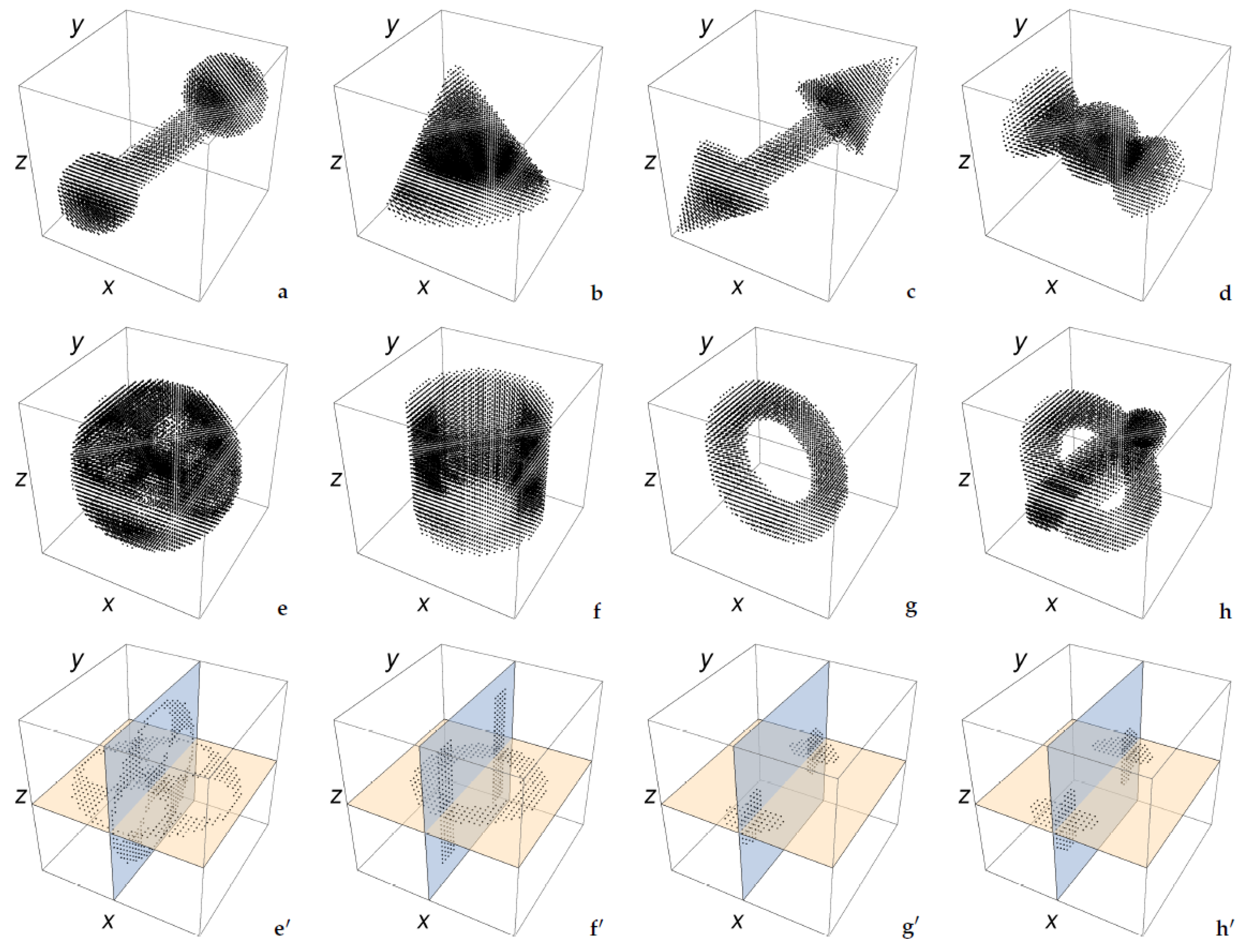
with element equal to 0 if the corresponding point is white (i.e., it belongs to the background) or equal to 1 if the point is black (i.e., it belongs to the foreground). Please note that these two colors are swapped with respect to the usual representation in order to improve the graphical rendering of the forthcoming figures (see
Figure 2).
Let
k be the total number of foreground points in the body to reconstruct. Each individual in the population is actually a binary vector of length
instead of
k three-dimensional coordinates. This choice may result in a potential waste of memory in the case of very few foreground points (i.e., sparse data) but it simplifies the genetic operators, which must be performed quickly.
Figure 3 shows the vector representation of the object in
Figure 2e.
We used no distinctive information regarding the final goal; therefore, the initial individuals are formed by completely random vectors, each containing k elements equal to 1 and the remaining elements equal to 0. Our experimental results confirm that a few generations are usually sufficient to approximate the searched solution, even in the case of small values of .
2.2. Projections
Traditionally, the tomographic reconstruction has been approached by using projections that cut the body, literally slicing and then reconstructing it. We preferred to reconstruct the whole body at once from twelve projections intended as complete “radiographs”—that is, from a few planar images representing the number of black points along the direction perpendicular to each radiograph. When a large number of projections is available, the complexity increases because the image has to satisfy more constraints, and it is also true that this reduces the presence of eventual artifacts. In this paper, constraints are retained by projections in the three-dimensional space along non-coplanar directions: the underlying idea is that these projections should not revolve around any axis.
Besides the natural direct access through coordinates to each point in the individual, we created a structure (essentially a lookup table of memory locations of about
MiB with
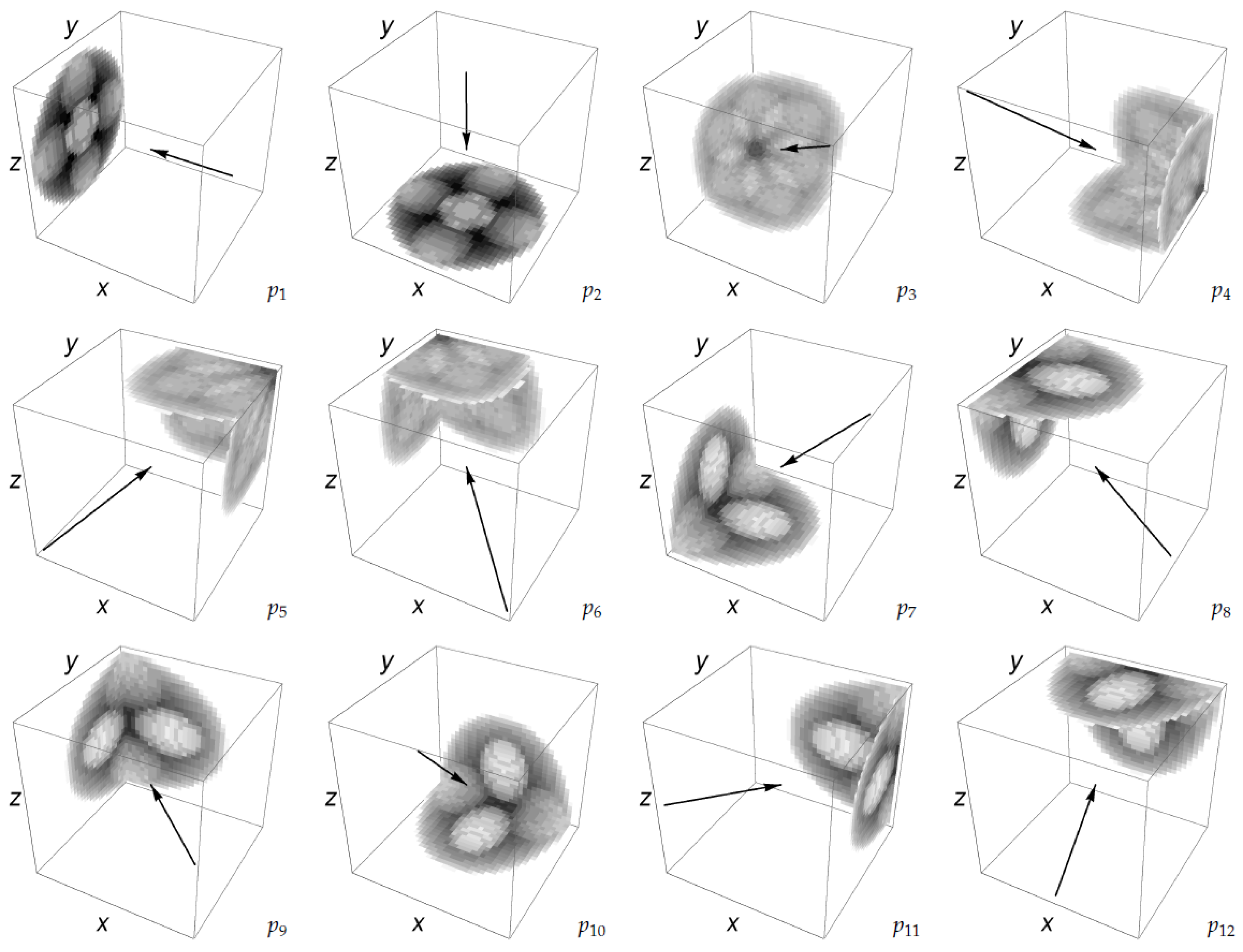
, respectively) that provides quick access to a whole projection plane by grouping all points that belong to it, arranged so as to reduce memory faults. We chose twelve particular projections (
Figure 4) because points along the same direction vector are adjacent to each other and because they make it easy to create the lookup data structure. An animation that we include in the supplementary material shows that the projection planes
vary in shape and size inside the cube, depending on both the angle and depth of the considered projection. As a complete example,
Figure 5 shows the projections of the object in
Figure 2e.
Crossover and mutation (to be described in
Section 2.4 and
Section 2.5) take most of the total processing time because each point modified in the individual’s encoding is picked up by all twelve projections, which must be updated. In the case of crossover, the entire object modifies radically and, therefore, recalculating the projections is mandatory. On the other hand, mutation affects a few points and just some parts of the projections should be updated; nonetheless, it is more convenient to recalculate all whole projections. To recalculate the projections as fast as possible, we make extensive use of the ordered coordinates in the lookup table. According to this data structure, we actually deal with all twelve projections of a given object as a numeric vector.
Figure 6 shows the projections in
Figure 5 and should not be mistaken with the binary vector illustrated in
Figure 3: the former is an example of input for our methodology whereas the latter is the corresponding output.
2.3. Fitness Function
Given an individual from the population, its fitness is merely the distance (i.e., the sum of the absolute value differences) between the individual’s projection vector and that provided as input. Better individuals correspond to lower fitness; a zero value indicates that the individual’s projections are identical to those of the object, although there is no guarantee that the two cubes are actually identical.
Despite its simplicity and fast computation, this fitness function provides enough variability to obtain correct results for all objects we considered. The population evolves until a stable solution is found or a maximum number of generations is reached.
2.4. Crossover
We considered several selection methods (e.g., tournament, ranking and roulette) to choose individuals for crossover, but they yielded poor results. As a consequence, we excluded them in the final version of the algorithm and the pair of individuals to recombine is randomly selected: this does not adhere strictly to the evolutionary theory, though it allows for more gene variability. Moreover, crossover occurs according to the probability , which is set by the user.
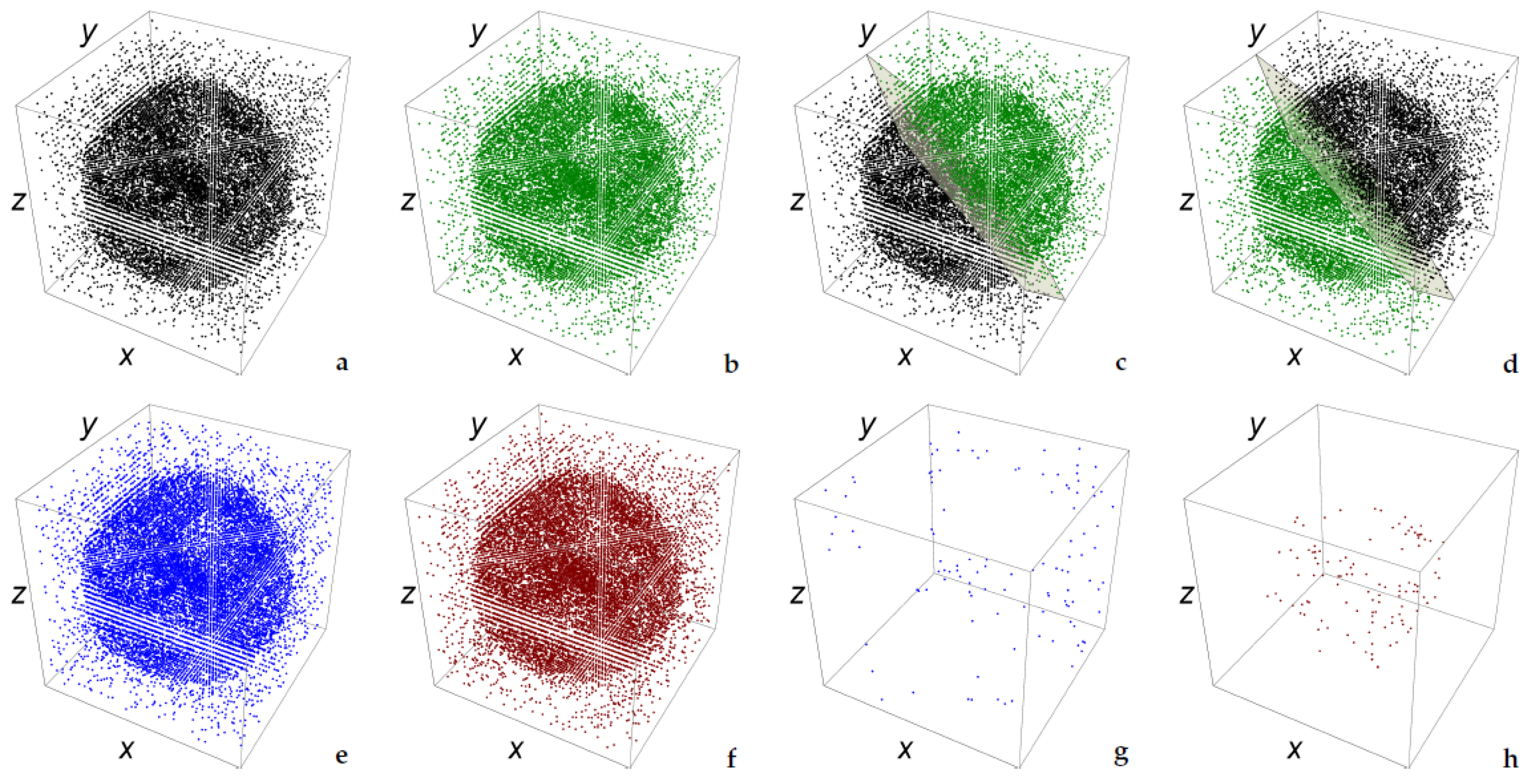
Given any point within the cube and one of the possible twelve projections directions, the crossover operator cuts both individuals (i.e., parents) along the plane passing through that point and orthogonal to that direction. Both the point and the direction are determined randomly. The parts of the cut individuals are swapped to obtain a couple of offspring; their new projections must be calculated completely. The individuals thus obtained generally possess an incorrect number of foreground points, but comparing their projections with the input ones allows us to add random points where they are missing and to eliminate them where they are in excess. This last step of the operator basically constitutes some form of mutation, although it is aimed at improving the fitness. The projections of the final individuals must be updated.
Figure 7 and
Figure 8 illustrate the crossover application on a couple of individuals attempting to reconstruct the object in
Figure 2e.
Parents and children are compared together based on their fitness values, and the two best ones remain in the future population to keep the population size constant throughout the whole process. This means that parents only are allowed to remain alive, as opposed to other techniques that replace parents with offspring in every case and regardless of their quality.
2.5. Mutation
This simple operator modifies the shape of an individual by changing the state of some of its points. The user specifies a priori the probability that an individual will undergo mutation, the amount of its points that will change from background to foreground, or vice versa. This allows finer control on the behavior of the genetic algorithm in relation to the number of individuals: in the case of a very small population, it is advantageous to have few mutating individuals (a small value of ), although the selected individuals must undergo a more pronounced mutation (a large value of ). It is noteworthy that indicates the exact number of points, meaning that during mutation it is not possible for the same point to change its state more than once. Usually, is much smaller than to guarantee a gradual convergence towards a stable solution within the search space.
As single isolated points (i.e., completely surrounded by points of opposite state) are generally attributed to noise, immediately after mutation we detect these isolated points and randomly choose them to change their state. Mutated points are chosen randomly and, therefore, the fitness of the new individual may be worse: an equal number of background and foreground points (actually, the minimum value between the quantity of these two sets of points) are exchanged to keep their total amount constant. This means that some isolated points may remain if the number of background and foreground is not equal. Regrettably, detecting isolated points is a particularly slow operation because it requires scanning each point within the cube through a sliding box with
points.
Figure 9 depicts an example of mutation.
2.6. Crossbreeding
Crossbreeding is about improving the biological quality of a hybrid progeny obtained by sharing traits from parents of different lineages. Although the resulting offspring may sometimes be inferior to the parents, this problem is overcome by the genetic algorithm that quickly removes unpromising individuals. One possible pattern involves sub-populations (named demes) evolving independently during most of the time; at regular generations, all individuals are merged to compete altogether and mix their genotype with individuals from other demes [
34].
When a deme remains isolated for a long time from the rest of the population, it may become a subspecies from the original population. In our case, each deme could converge independently to different solutions of the same problem, and this constitutes an implicit form of computational parallelism. From a practical point of view, we require that each deme evolves its gene pool independently of one another (thus covering different areas of the search space) and that in every generation the demes share information to converge toward a common best solution.
From
Section 2.4, it is clear that a simple method of randomly choosing pairs of individuals to crossover is to shuffle randomly the population at the beginning of each generation. This is performed directly with a random permutation of
integers, representing the indices of individuals in the entire population. So far, this corresponds to merging all the demes.
Let us consider each deme of equal size
, where
is the number of demes. To separate the demes, it is sufficient to assemble a permutation of
integers that has the indexes from 1 to
in the first
elements, the indexes from
to
in the elements from
to
, the indexes from
to
in the elements from
to
and so on (
Figure 10).
Basically, these demes remain alone for most of the time by way of this particular permutation; every generations, a totally random permutation of length merges them all together, thereby allowing individuals to migrate among them. From a computational perspective, the application of crossbreeding does not involve any real overhead with respect to the rest of the methodology.
2.7. Cloning
This is the ordinary elitist selection that assures that only the individual with the best fitness value will be present as two identical copies in the next population. In the case of demes, cloning is applied to each sub-population.
Usually, this reduces the variability of the hereditary characteristics in the case of very few individuals; nonetheless, we have experimentally verified that this strategy increases the accuracy of the final result when enough individuals are available.
3. Results
In order to verify the effectiveness of the proposed genetic algorithm, we produced twenty objects of different shapes with
,
and
points, sometimes composed by more than one part or with hollows inside them. Some instances have been shown in
Figure 2.
We limited the preliminary experiments to ; ; ; ; ; ; and when . This leads to 243 experiments per object. In addition, to minimize the effect of random fluctuations, each set of parameters was evaluated five times (i.e., 1215 experiments per object).
Despite the typical uncertainty of evolutionary approaches, all experiments returned correct results: not only were the final projections identical to the initial ones, but the reconstructed objects were actually identical to those satisfying the initial projections. Hence, the processing time alone can be used to identify the optimal values of parameters.
The application of crossover can be reduced as the number of individuals increases: with , it is appropriate to use , respectively. On the other hand, we have already discussed how the computation time is linearly dependent on the number of individuals.
Regarding mutation, we have experimentally verified that the values and are the most convenient, independent of the number of individuals, thus confirming the importance of genetic diversity. In other words, it is advisable to mutate just a few individuals greatly.
Crossbreeding is irrelevant with individuals because not enough gene diversity is available; instead, with individuals, it is useful to merge demes every generations.
We observed that the shape complexity of the object, which is difficult to formalize in rigorous terms, influences the computation time, whereas the mere number of points that compose the object does not modify so much the convergence rate towards the solution.
We almost always obtained the exact reconstruction of the object with individuals, making it useless to work with or even individuals; this entails a significant gain in processing time. However, it is suggested to increase the number of individuals to compute the position of a large number of points or when the object consists of various components. We considered this possibility in the conclusion below.
Ultimately, the parameters that correspond to the best trade-off between convergence speed and correctness of the solution are, in general,
Figure 11 shows the
average trend in reconstructing the objects in
Figure 2 with this set of parameters. In the additional material, we provide animations for
single reconstructions of the objects in
Figure 2e–
h.
Our algorithm was implemented in MatLab 2017b language for Windows 10 on an i7-2600 processor (produced in 2011) with 16 GiB of RAM. Although some experiments with points and with individuals took just five seconds, the average time was about thirty seconds. A single experiment with individuals takes about four minutes when and more than half an hour when . These times roughly double in the case and more than quadruple in the case .
Altogether, the initial 24300 experiments (i.e., 1215 experiments for 20 objects) with just required about three weeks. To make sure that the default parameters are indeed also the best in the case of and because the exhaustive completion of all experiments (i.e., with ) would take approximately four years, we performed further experiments with only the prefixed parameters plus 1% of random tests of the remaining experiments (corresponding to two weeks or so of calculations). Limited to the parameter values we considered, the search for the default ones is exhaustive in the case and extended to the cases. All these evaluations confirmed the correctness of the default above parameters. Regarding the hardware we used, we expect that the latest generation i7 CPU with current RAM should provide just half the calculation time.
4. Discussion
Discrete tomography differs from standard computerized tomography in the small variety of density distribution of the object to analyze and in the very few projections to take. Although this research field is now more than thirty years old, it is still particularly complex to address, and the increasing number of recent publications highlights a great interest because of the variety of possible practical applications.
The methodology we presented here is able to compute in a reasonable amount of time the reconstruction of three-dimensional binary objects from twelve projections: about 30 s for a cube of points, which corresponds to a traditional slice of pixels. Our evolutionary approach is simple and exhibits great flexibility because no model (e.g., periodicity, convexity or symmetry) is needed. To the best of our knowledge, this is the first discrete tomography algorithm able to deal with this type of reconstruction directly.
We were interested mainly in the development of reconstruction techniques, albeit in an efficient way on regular personal computers rather than in optimizations on particular hardware. In practice, we proved that it is possible to extend binary discrete tomography to the three-dimensional case with a sufficiently fast computing time.
It can be argued that twelve projections are more than what is usually proposed for the reconstruction in discrete tomography. We would like to emphasize that we use these projections for a direct reconstruction of three-dimensional objects of any shape—that is, without assuming any particular model. Indeed, many algorithms proposed in the literature use fewer projections to deal with planar reconstructions provided that it is given some information about the final appearance of the binary image.
The bottleneck of the proposed reconstruction methodology lies in accessing the three-dimensional coordinates of the points, basically as a function of the direction of the radiation considered. As described in
Section 2.1, the shape of the plane orthogonal to this direction changes together with the position of the point itself. Due to this reason, we have precomputed all spatial coordinates, although this requires a large amount of memory in the case of big cubes.
Evolutionary algorithms are particularly suitable to exploit parallel implementations. Our code was written from scratch in MatLab language without even using its Global Optimization Toolbox. Except for the native parallelism offered by this vector programming language, no parallel instructions (multi-core CPU either GPU) have been applied explicitly. This should ease the translation of our methodology onto heterogeneous, high-performance machines by implementing in parallel all operations that can be subdivided into simpler steps to be performed independently of each other.


