Article

Finite-Time Fault-Tolerant Control of Nonlinear Spacecrafts with Randomized Actuator Fault: Fuzzy Model Approach

1
Internet of Things Department, Henan Institute of Economics and Trade, Zhengzhou 450000, China
2
College of Control Science and Engineering, Zhejiang University, Hangzhou 310058, China
3
School of Electrical and Electronic Engineering, Nanyang Technological University, Singapore 639798, Singapore
4
College of Automation, Chongqing University, Chongqing 400044, China
*
Author to whom correspondence should be addressed.
Symmetry 2024, 16(7), 873; https://doi.org/10.3390/sym16070873
Submission received: 4 June 2024 / Revised: 23 June 2024 / Accepted: 3 July 2024 / Published: 9 July 2024
(This article belongs to the Section Engineering and Materials)

Abstract

:
The primary objective of this paper is to address the challenge of designing finite-time fault-tolerant control mechanisms for nonlinear flexible spacecraft systems, which are particularly vulnerable to randomized actuator faults. Diverging from traditional methodologies, our research harnesses the capabilities of the Takagi–Sugeno (T–S) fuzzy framework. A unique feature of our model is the representation of actuator failures as stochastic signals following a Markov process, thereby offering a robust solution for addressing timeliness concerns. In this paper, we introduce a generalized reciprocally convex inequality that includes adjustable parameters, broadening the scope of previous results by accommodating them as special cases. Through the amalgamation of this enhanced inequality and flexible independent parameters, we propose an innovative controller design strategy. This approach establishes a stability standard that guarantees mean-square H performance. In order to validate the efficacy of the suggested strategy, we present a numerical illustration involving a nonlinear spacecraft system, showcasing the practical advantages and feasibility of our proposed technique.

1. Introduction

In recent decades, a noteworthy surge in scholarly endeavors has been witnessed, focusing on addressing the stabilization challenges associated with flexible spacecraft systems [1,2]. This surge is evidenced by a growing body of research. The increased interest in this field is primarily driven by the growing recognition of the substantial advantages that flexible spacecraft systems offer in the realm of space activities. A closer examination of attitude control systems for flexible spacecraft reveals a complex and demanding landscape. These systems exhibit intricate dynamics, characterized by robust interconnections between flexible and rigid modes [3,4]. Moreover, the precise values of key parameters governing these nonlinearities, along with several other system parameters, often elude accurate measurement and characterization. These inherent nonlinearities and uncertainties not only present a formidable challenge in designing control strategies but also exert a discernible impact on the overall system performance.
A well-established approach to addressing such complex nonlinearities involves the utilization of fuzzy system models [5,6]. Fuzzy models excel in their capacity to approximate unparameterized functions with nonlinearity through a linearly parametrized representation, thereby achieving suitably small approximation errors [7,8]. In recent years, this methodology has yielded numerous effective control strategies tailored to address the intricate dynamics of various nonlinear systems. These advances are primarily rooted in the T–S fuzzy model framework. In the research conducted by [9], the focus was on addressing the complexities of event-triggered control through the application of an H strategy to a truck-trailer model. The study utilized the T–S fuzzy model approach to ensure system stability. Academic work [10] employed a sophisticated Lyapunov technique to design an output feedback controller for an interval type 2 T–S fuzzy system, considering the impact of external disturbances. It is vital to underscore the significance of actuators in control systems, as their failure can lead to subpar performance or even cause the system to become unstable. This is especially critical in the context of space vehicles, where the emphasis on reliability is extremely high. A decrease in the working efficiency of space vehicles due to actuator issues could potentially result in fatal accidents. As a result, there is an increasing focus on developing dependable control systems that can counteract actuator faults, ensuring robustness and high reliability, not just in space vehicles but also in industrial systems. However, it is important to note that many existing reliable control methodologies are based on the assumption that faults are deterministic. In practical scenarios, faults can exhibit both predictable and random characteristics, often due to elements such as wear and tear or harm to control parts. To address this intricacy, contemporary studies have investigated diverse strategies to handle unpredictable actuator faults. For example, in the paper [11], researchers tackled the problem of output feedback H control in nonlinear spatially distributed systems affected by Markovian jump-type actuator faults. A robust feedback control strategy for T–S fuzzy systems, affected by sensor multiplicative errors, was developed using the dynamic parallel distributed compensation technique [12]. A new T–S fuzzy controller was developed, tailored specifically for spacecraft dealing with random actuator defects. The researchers in [13,14] aimed to tackle the issues brought about by actuator faults by implementing a restriction condition, specifically to acheive H performance. Conversely, in another methodology [15], a distinct stabilization technique was employed to address the problems caused by actuator faults. This approach incorporated an innovative iterative linearization algorithm for the design of controller gains. Furthermore, in the research conducted by [16], the issue of finite-time control in a nonlinear flexible spacecraft system affected by random errors was investigated. However, the said study mainly employs Jensen’s inequality and transforms time-varying delays into maximum limits, which brings about substantial conservatism. Hence, it is essential to investigate novel techniques to enhance the application of time-varying delays [17,18].
In addition, the traditional H stabilization strategy is often utilized to scrutinize the preferred behavior of considered dynamics and investigate the asymptotic properties of controlled system trajectories, generally assuming an infinite time stability theory [19,20]. In practical scenarios, the focus often lies on the behavior of dynamic systems within a specific, limited time frame. For instance, there might be situations where the impact of external disturbances requires a guarantee that the system’s states stay within acceptable boundaries during this finite period [21,22]. In these scenarios, the principle of finite-time boundedness gains paramount significance. The past several years have seen a surge in attention towards this principle, backed by extensive studies and related refs. [23,24,25]. In this research, the method of free-weighting matrices is commonly employed, typically necessitating the inclusion of auxiliary matrices. Yet, it is vital to recognize that the adaptability of these supplementary matrices is intrinsically limited, suggesting a possible scope for improvement.
This paper investigates finite-time fuzzy fault-tolerant control for spacecraft mechanisms under the influence of actuator malfunctions, employing the T–S fuzzy paradigm. Unlike traditional methods, actuator malfunctions are represented as random signals following a stochastic Markov process, offering a comprehensive solution to concerns related to timeliness. A generalized reciprocally convex inequality with tunable parameters is introduced, which includes existing results as special cases. By integrating this enhanced inequality with flexible independent parameters, this novel controller design methodology formulates a less conservative H performance analysis condition in a mean-square sense compared with some existing works [13,14]. The effectiveness of this approach is empirically validated through a numerical example involving a fuzzy spacecraft system, demonstrating the practical applications and benefits of the proposed methodology. To enhance the flexibility of the control approach, a set of versatile parameters is incorporated. This novel controller design technique permits individual modification of these variables, offering a higher level of autonomy and personalization relative to current approaches. Significantly, these adaptable variables are predetermined, distinct from the unidentified slack matrices observed in prior research [13,16]. When compared with previous literature like [13,16], this control strategy demonstrates enhanced usability and efficacy.
The rest of this paper is organized as follows. Section 2, gives the system description and preliminaries. In Section 3, the main results are given. Section 4 provides a numerical example, and Section 5 concludes the paper.
Notation: The sum of A and its transpose is denoted as [ A ] s or A s . The symbol ⨂ is used to denote the Kronecker product for matrices. Unless explicitly stated, matrices are assumed to have compatible dimensions.

2. System Description and Preliminaries

Figure 1 illustrates the overall closed-loop dynamical system’s structure. The motion and forces of the pliable spacecraft are characterized by differential equations. To represent the rotational state of the spacecraft, quaternion notation is introduced. We set α 0 = cos ( v 2 ) and the quaternion vector can be defined as α = [ α 1 , α 2 , α 3 ] T = Λ sin ( v 2 ) . It is important to note that the constraint i = 0 3 α i 2 = 1 must be satisfied. The dynamic model of this nonlinear spacecraft model can be denoted as follows:
α ˙ 0 = 1 2 α T β ( t )
α ˙ = 1 2 ( α 0 I + H ( α ) ) β ( t )
G s β ˙ ( t ) + δ T ζ ¨ ( t ) = v ( t ) + j ( t ) H ( β ( t ) ) × ( G s β ( t ) + δ T ζ ˙ ( t ) )
ζ ¨ ( t ) + A s ζ ˙ ( t ) + F s ζ ( t ) = δ β ˙ ( t )
where for i = 1 , 2 , , n ˜ , let us define A s as the diagonal matrix
A s = d i a g { 2 ζ 1 β n 1 , 2 ζ 2 β n 2 , , 2 ζ n ˜ β n n ˜ }
and the diagonal matrix F s is defined as F s = d i a g { β n 1 2 , β n 2 2 , , β n n ˜ 2 } . Here, ζ i denotes the damping ratio for the i mode, v signifies the rotation angle about the Euler axis. The frequency for the ith mode is denoted by β n i , and β i (for i = 1 , 2 , 3 ) is associated with the pitch, yaw, and axis angular velocities, in that order. The matrix δ is responsible for coupling, and n ˜ denotes the total count of mode frequencies. The system’s control input is denoted by v ( t ) , and j ( t ) signifies an external disruption variable.
To simplify the representation, we can define a consolidated disturbance term since δ T ζ ¨ ( t ) , δ T ζ ˙ ( t ) , and δ T β ˙ ( t ) are interrelated. This consolidated disturbance term can be expressed as follows:
α ˜ ( t ) = j ( t ) + δ T ( A s ζ ˙ ( t ) + F s ζ ( t ) ) H ( β ( t ) ) δ T ζ ˙ ( t )
Recalling (3) and (4), one has
( G s δ T δ ) β ˙ ( t ) = H ( β ( t ) ) G s β ( t ) + v ( t ) + j ˜ ( t )
where G s is a positive definite matrix, δ indicates the coupling matrix with a sufficiently small norm.
Given that the condition 0 T j ˜ T ( t ) j ˜ ( t ) j ˜ holds true for j ˜ ( t ) L 2 [ 0 , T ] . The state vector can be defined as follows: χ T = [ χ β T , χ α T ] T = [ β 1 , β 2 , β 3 , α 1 , α 2 , α 3 ] T . Here, α denotes the quaternion, and β signifies the angular rate, both are viewed as the regulated outputs. By amalgamating Equations (1) through (5), the dynamic system is obtained by an “IF-THEN” fuzzy principle.
Rule i: IF { ϵ 1 ( t ) is N 1 i } , { ϵ 2 ( t ) is N 2 i } , …, { ϵ η ( t ) is N l i } , THEN
χ ˙ ( t ) = A i χ ( t ) + B i v ( t ) + B i j ˜ ( t ) p ( t ) = C i χ ( t )
We define ϵ T ( t ) = [ ϵ 1 ( t ) , ϵ 2 ( t ) , , ϵ n ( t ) ] T , and N j 1 ( j = 1 , 2 , , η ) are recognized as T–S fuzzy sets. Here, the expression of the system matrices, denoted as A i , B i , and C i can be delineated in the subsequent manner:
A i = ( G s δ T δ ) 1 H ( χ β i ) G s 0 1 2 1 | | χ α i | | 2 I 1 2 H ( χ β i ) B i = ( G s δ T δ ) 1 0 , C i = I .
Hence, the T–S fuzzy system can be delineated as
χ ˙ ( t ) = A i χ ( t ) + B i v ( t ) + D i j ˜ ( t ) p ( t ) = C i χ ( t )
where
h i ( ϵ ( t ) ) = φ i ( ϵ ) / i = 1 r φ i ( ϵ , h i ( ϵ ( t ) ) > 0 φ i ( ϵ ( t ) ) = j = 1 η M j i ( ϵ j ( t ) ) , i = 1 r h i ( ϵ ( t ) ) = 1 .
Remark 1. 
It should be clarified that the set of fuzzy rules employed in this study is meticulously designed to cover all possible operational scenarios of the nonlinear spacecraft system. Consequently, each rule is crafted to address distinct conditions, ensuring that the control logic is exhaustive in the sense that at least one rule is always applicable, as seen in [13,14,21]. For instance, within the context of Rule 1, should the premise conditions not be met, the system seamlessly transitions to assess subsequent rules. This approach guarantees that the system’s response is consistently governed by the most pertinent rule, thereby preserving the integrity and performance of the control system.
The sensor grid intercepts system output signals, employing an output feedback technique for the formulation of the controller. In actual systems, the output vector p ( t ) is periodically sampled at set t 0 , t 1 , , t k , t k + 1 , via a sampling device. This discretely sampled output signal is then directed into the input interface of the sensor network. In controller design, signals from the system’s output are captured by the sensor network using an output feedback method. It is important to note that at a specific sampling point, say t k , the value of p ( t k ) stays constant during the time interval [ t k , t k + 1 ) . Therefore, the signal that the sensors receive during this interval, i.e., for t [ t k , t k + 1 ) , is consistently represented by p ( t k ) .
It is important to underscore that the components of the adjacency matrix should be positive for the edges present in the graph, which is expressed as θ i j 0 for all ( i , j ) E . Moreover, for nodes belonging to V , the diagonal elements of the matrix Θ are determined as l 2 = 1 , l 2 l 1 m θ l 1 l 2 .
The ideal control input is
v ( t ) = F i z ( t k )
the output of the l 2 t h sensor is given by z l 2 ( t k ) = l 1 = 1 m θ l 1 l 2 y ( t k ) and z t k = l 2 = 1 m z l 2 ( t k ) . Here, L l 2 denotes the output matrix of the l 2 -th sensor, and θ satisfies the corresponding limit.
θ l 1 l 2 0 , if l 1 l 2 θ l 1 l 2 = l 2 = 1 , l 2 l 1 m θ l 1 l 2
This paper considers a situation where the sampling intervals are not periodic but remain bounded. This means that between successive sampling points, one has 0 < t k + 1 t k τ k τ M . Define τ ( t ) = t t k to represent the elapsed time from the previous sampling point t k . It is crucial to observe that τ ( t ) complies with the condition 0 τ ( t ) τ M and τ ˙ ( t ) = 1 for all instances, barring the distinct sampling point t = t k .
Taking into account randomized failures, we have
v f ( t ) = F r ( t ) v ( t ) + G r ( t ) u ( t )
Here, u ( t ) can be seen in (7), v ( t ) is a bounded actuator fault. For scalar u ¯ , u ( t ) can be denoted as 0 T u T ( t ) u ( t ) d t u ¯ . Moreover, the fault matrices can be defined as F r ( t ) and G r ( t ) , where F r ( t ) = d i a g ( f ψ ( r ( t ) ) ) for ψ = 1 , , n . The stochastic Markov process can be denoted by r t ( t 0 ) , which satisfies
Π = [ π i j ]
and transition rates can be denoted as follows:
P r { r t + f = j | r t = i } = π i j f + o ( f ) , j i 1 + π i i f + o ( f ) , j = i
where π i j 0 and π i i = j = 1 , j i N π i j 0 .
In order to streamline the symbols, we establish F r = F ( r ( t ) ) , f r ψ = f ψ ( r ( t ) ) , and likewise for G r with g r ψ in { 0 , 1 } . In addition, in Equation (8), we set the constraints 0 f ̲ r ψ f r ψ f ¯ r ψ 1 , where f ̲ r ψ and f ¯ r ψ respectively denote the lower and upper bounds of f r ψ . Defining F ̲ r = d i a g { f ̲ r ψ } , F ¯ r = d i a g { f ¯ r ψ } , F r 0 = F ̲ r + F ¯ r 2 , and F r 1 = F ¯ r F ̲ r 2 , F r can be depicted as the amalgamation of F r 0 and F r 1 scaled by r , where r is defined as d i a g { σ r 1 , σ r 2 , , σ r n } with 1 σ r ψ 1 .
By amalgamating (6) and (8), we put forth the subsequent fuzzy FTC methodology. This controller, under the influence of the sampled-data input, is architected as follows:
Rule i: IF { ϵ 1 ( t k ) is N 1 i } , { ϵ 2 ( t k ) is N 2 i } , …, { ϵ η ( t k ) is N l i } , THEN
v f ( t ) = j = 1 p h j ( ϵ ( t k ) ) { F r F r j l 1 = 1 m l 2 = 1 m θ l 1 l 2 L l 2 p ( t k ) + G r u ( t ) } , t [ t k , t k + 1 )
where F r j is the required controller.
Setting h i j = i = 1 p j = 1 p h i ( ϵ ( t ) ) h j ( ϵ ( t k ) ) and θ l 12 = l 1 = 1 m l 2 = 1 m θ l 1 l 2 , combining (10) and (6), we can derive the following dynamical system:
χ ˙ ( t ) = h i j [ A i χ ( t ) + B i F r F r j θ l 12 L l 2 C i χ ( t τ ( t ) ) + B i G r v ( t ) + D i j ˜ ( t ) p ( t ) = h i j C i χ ( t )
Furthermore, by recognizing that B i F r F r j θ l 12 L l 2 = B i F r F r j I T q m ( Θ I q ) L C i χ ( t τ ( t ) ) , model (11) can be rewritten as
x ˙ ( t ) = h i j [ A i χ ( t ) + B i F r F r j I q m T ( Θ I q ) × L C i χ ( t τ ( t ) ) + B i G r u ( t ) + D i j ˜ ( t ) p ( t ) = h i j C i χ ( t )
where I q m T = [ I q , I q , , I q ] m and L = [ L 1 , L 2 , , L m ] T .
In our pursuit of addressing the challenge of fuzzy FTC control with stochastic actuator faults, our chief aim is to architect a fuzzy fault-tolerant controller that meets the subsequent performance benchmarks:
(i) Given the positive scalars a 1 , a 2 , τ M , β ¯ , T , and a positive definite matrix Z, we can ascertain that system (12) demonstrates FTSDB in relation to the parameters ( a 1 , a 2 , τ M , β ¯ , T , M ) , provided certain prerequisites are met:
sup τ U s 0 E [ χ T ( s ) Z χ ( s ) , χ ˙ T ( s ) Z χ ˙ ( s ) ] a 1 E [ χ T ( t ) Z χ ( t ) ] < a 2 , t [ 0 , T ]
(ii) For positive values of T > 0 and γ > 0 , if the subsequent condition is satisfied, then system (12) attains the H performance level:
0 T γ 2 β T ( s ) β ( s ) p T ( s ) p ( s ) d s > 0
By defining β ( s ) [ u T ( s ) , j ˜ T ( s ) ] T and imposing the constraint 0 T β T ( s ) β ( s ) d s u ¯ + j ¯ β ¯ , we construct a strategy that employs the captured output from an individual sensor and its adjacent sensors. This innovative technique presents a distinctive condition for preserving system stability and concurrently attaining H performance. Furthermore, we develop a procedure for formulating controller gains that satisfy these particular criteria.

3. Main Results

Thus far, the Lyapunov stability analysis technique has been widely employed in the creation of controllers for delay systems due to its adaptability across diverse scenarios. This approach has been the foundation for the primary conclusions of this study. As we develop the FTC method, we will present two fundamental preconditions.
Lemma 1. 
[26] Assuming the constants γ 2 , γ 1 , where γ 2 > γ 1 > 0 , along with Z > 0 , and the variable χ: [ γ 1 , γ 2 ] × R n R n , the following holds:
( γ 2 γ 1 ) γ 1 γ 2 χ T ( p ) Z χ ( p ) d p γ 1 γ 2 χ T ( p ) d p Z γ 1 γ 2 χ ( p ) d p
Lemma 2. 
For real scalars α 1 , α 2 ( 0 , 1 ) with the constraint α 1 + α 2 = 1 and real symmetric positive definite matrices Z R m × m , along with κ 1 1 and κ 2 1 , if there exist real matrices Y 1 , Y 2 R m × m , then the following matrix inequality is valid:
τ M t τ M t χ ˙ T ( p ) Z χ ˙ ( p ) d p ξ 1 T [ ( 1 + κ 1 α 2 ) Z κ 1 α 2 Y Z 1 Y T ) ] ξ 1 + 2 ξ 1 T Y ξ 2 + ξ 2 T [ ( 1 + κ 2 α 1 ) Z κ 2 α 1 Y T Z 1 Y ) ] ξ 2
where ξ 1 = x ( t τ ( t ) ) χ ( t ) and ξ 2 = x ( t τ M ) x ( t τ ( t ) ) .
Proof. 
Based on Lemma 1, it yields
τ M t τ M t χ ˙ T ( p ) Z χ ˙ ( p ) d p τ M τ ( t ) ξ 1 T Z ξ 1 + τ M τ M τ ( t ) ξ 2 T Z ξ 2
Set α 1 = τ ( t ) τ M and α 2 = τ M τ ( t ) τ M , one has
1 α 1 ξ 1 T Z χ 1 + 1 β ξ 2 T Z χ 2 ξ 1 T [ Z + α 2 κ 1 ( Z Y Z 1 Y T ) ] ξ 1 + ξ 2 T ( Z + α 1 κ 2 ( Z Y T Z 1 Y ) ) ξ 2 + 2 ξ 1 T Y ξ 2 .
Arranging it, one has (14). This completes the proof. □
Remark 2. 
In comparison to the existing reciprocally convex inequality, Lemma 2 depends on two parameters, κ 1 and κ 2 , which it generalizes. Therefore, it can be termed as the generalized reciprocally convex inequality (GRCI). The advantages of GRCI are twofold:
(i) Two prespecified parameters, κ 1 and κ 2 , lead to the derivation of a more stringent reciprocally convex inequality without the introduction of additional decision variables.
(ii) In contrast to the traditional reciprocally convex inequalities with a predetermined parameter α ( 0 , 1 ) , the two parameters, κ 1 and κ 2 , in GRCI are not constrained. This allows for their selection without limitations, facilitating the pursuit of less conservative stability conditions when needed.
Lemma 3. 
[13] Assuming P, Q, and R, if it is the case that | | Q | | 1 exists, then for any ϵ greater than zero, the subsequent requirement is satisfied:
[ P Q R ] s ϵ 1 P P T + ϵ R T R
Theorem 1. 
Assuming the scalar quantities κ 1 , κ 2 , positive scalars α , γ , τ M , c 1 , and H, system (12) is capable of exhibiting FTSDB in relation to the variables ( c 1 , c 2 , τ M , w ¯ , d ^ , T , H ) . Furthermore, it can fulfill the H performance standard given the existence of scalar quantities c 2 , ρ 1 , P r l > 0 , Q > 0 , R > 0 , W > 0 , Z i j > 0 , and matrices U 1 , U 2 , such that the following matrix inequality is met for any 1 i j p :
Ω i j 1 Y i j Ω i j 2 κ 2 I 14 τ ( t ) Y T I 14 T * Z i j 0 0 * * τ M R 0 * * * τ M R < 0
Ω i j 0.5 Y i j Ω i j 2 κ 2 I 14 τ ( t ) Y T I 14 T * Z i j 0 0 * * τ M R 0 * * * τ M R < 0
e α T { c 1 [ μ 1 + μ 2 μ ] + 2 ( c 1 μ 3 + d ^ ) μ + γ 2 β ¯ } < c 2 m u 0
where Ω i j ( e 0.5 α τ ( t ) ) = [ φ s l ] 5 × 5 and
Ω i j 1 = 1 2 ( Ω i j ( 1 ) + Ω i j ( 1 ) ) + X i j Z i j X i j T Ω i j 0.5 = 1 2 ( Ω i j ( e 0.5 α τ M ) + Ω i j s l ( e 0.5 α τ M ) ) + X i j Z i j X i j T Ω i j 2 = κ 1 I 13 ( τ M τ ( t ) ) Y I 13 T μ 0 = μ m i n ( 1 ρ 1 2 P ˜ r ) , μ 1 = μ m a x ( P ˜ r ) μ 2 = μ m a x ( Q ˜ ) , μ 3 = μ m a x ( R ˜ ) P ˜ r = ρ 1 2 H 1 2 P r H 1 2 , Q ˜ = ρ 1 2 H 1 2 Q H 1 2 R ˜ = ρ 1 2 H 1 2 A i R A i H 1 2 μ = e α τ M 1 α , μ = e α τ M α 2 1 α 2 τ M α 2 φ 11 = Q α P r ( 1 + κ 1 ( τ M τ ( t ) ) τ M ) R π 2 4 τ M 2 W + C i T C i + U 1 T A i + A i T U 1 + h = 1 N π r h P h φ 12 = P r l U 1 T + A i T U 2 φ 13 = ( 1 + κ 1 ( τ M τ ( t ) ) τ M ) R Y + e 0.5 α τ ( t ) π 2 4 τ M 2 W + ε 1 U 1 T B i F r F r j I q m T ( Θ I q ) L C i φ 14 = Y , φ 15 = U 1 T D i + U 1 T B i G r φ 22 = τ M R U 2 T U 2 + W φ 23 = U 2 T B i F r F r j I q m T ( Θ I q ) L C i φ 25 = U 2 T D i + U 2 T B i G r φ 33 = ( 1 + κ 1 ( τ M τ ( t ) ) τ M ) R + 2 Y ( 1 + κ 2 τ ( t ) τ M ) R e α τ ( t ) π 2 4 τ M 2 W , φ 34 = ( 1 + κ 2 τ ( t ) τ M ) R Y φ 44 = e α τ M Q ( 1 + κ 2 τ ( t ) τ M ) R , φ 55 = γ 2 I n X i j = ε 1 ( B i + B j ) T 2 [ U 1 , U 2 , 0 ] T [ I , I , , I ] r Y i j = [ 0 , I , 0 ] [ ( C i + C j ) 2 L T ( Θ I q ) T I q m F r 1 T F r T , , ( C i + C j ) 2 L T ( Θ I q ) T I q m F r p T F r T ] I 13 = [ I , 0 , I , 0 , 0 ] , I 14 = [ 0 , 0 , I , I , 0 , 0 ] .
Proof. 
We can construct the Lyapunov functional as follows:
V ( t , r t ) = i = 1 4 V i ( t , r t )
where
V 1 ( t , r t ) = χ T ( t ) P r χ ( t ) V 2 ( t , r t ) = t τ M t e α ( t p ) χ T ( p ) Q χ ( p ) d p V 3 ( t , r t ) = t τ M t β t e α ( t p ) χ ˙ T ( p ) R χ ˙ ( p ) d s d β V 4 ( t , r t ) = t k t d d p ( e 0.5 α ( t p ) χ ( p ) ) T W ( e 0.5 α ( t p ) χ ( p ) ) d p π 2 4 τ M 2 t k t ( e 0.5 α ( t p ) χ ( p ) e 0.5 α ( t t k ) χ ( t k ) ) T × W ( e 0.5 α ( t p ) χ ( p ) e 0.5 α ( t t k ) χ ( t k ) ) d s
Letting L be the weak infinitesimal generator along the stochastic Markov distribution (12), we thus arrive at the following result:
L V 1 ( t , r t ) = 2 χ T ( t ) P r χ ˙ ( t ) + χ T ( t ) [ j = 1 N π r j P j ] χ ( t )
L V 2 ( t , r t ) = α V 2 ( t , r t ) + χ T ( t ) Q χ ( t ) e α τ M χ T ( t τ M ) Q ( t τ M ) + τ M χ ˙ T ( t ) R χ ˙ ( t ) e α τ M χ ˙ T ( t ) R χ ˙ ( t ) t τ M t e α ( T S ) χ ˙ T ( s ) R χ ˙ ( s ) d s + χ ˙ T ( t ) W χ ˙ ( t ) π 2 4 τ M 2 [ χ ( t ) e 0.5 α ( t t k ) χ ( t k ) ] T × W [ χ ( t ) e 0.5 α ( t t k ) χ ( t k ) ] .
By Lemma 2, we establish a lower bound for t τ M t χ ˙ T ( p ) R χ ˙ ( p ) d p as follows:
t τ M t x ˙ T ( p ) R x ˙ ( p ) d p 1 τ M { χ 1 T ( R + κ 1 τ M τ ( t ) τ M ( R Y R 1 Y T ) χ 1 + 2 χ 1 T Y χ 2 + χ 2 T ( R + κ 2 τ ( t ) τ M ( R Y T R 1 Y ) χ 2 }
where χ 1 = χ ( t τ ( t ) ) χ ( t ) and χ 2 = χ ( t τ M ) χ ( t τ ( t ) ) .
For U 1 , U 2 and any free parameters ε 1 , ε 2 , it yields
2 { χ ˙ ( t ) i = 1 p i = 1 p h i ( ϵ ( t ) ) h j ( ϵ ( t k ) ) [ A i χ ( t ) + B i F r F r j I q m T ( Θ I q ) L C i χ ( t k ) + B i G r u ( t ) + D i d ˜ ( t ) ] } U T ζ ( t ) = 0
where U = [ ε 1 U 1 , ε 2 U 2 , 0 , 0 , 0 ] T , ζ = [ χ T ( t ) , χ ˙ T ( t ) , χ T ( t τ ( t ) ) , χ T ( t τ M ) , β T ( t ) ] T .
With the above procedure, it yields:
L V ( t , r t ) γ 2 β T ( t ) β ( t ) + p T ( t ) p ( t ) i = 1 p j = 1 p h i ( ϵ ( t ) ) h j ( ϵ ( t k ) ) ζ T ( t ) Ω i j ζ ( t ) + α V ( t , r t )
Setting ϵ j ( ϵ ( t ) ) = h j ( ϵ ( t k ) ) h j ( ϵ ( t ) ) , k = 1 p ϵ ( ϵ ( t k ) ) = 0 , it yields
X i j Z i j X i j T + Y i j Z i j 1 Y i j T + 1 τ M κ 1 I 13 ( τ M τ ( t ) ) Y R 1 Y T I 13 T + 1 τ M κ 2 I 14 τ ( t ) Y T R 1 Y I 14 T ϵ i j
where
U 1 = U 1 T B i + B j 2 F r F r k I q m T ( Θ I q ) L C i + C j 2 U 2 = U 2 T B i + B j 2 F r F r k I q m T ( Θ I q ) L C i + C j 2 Γ ( ϵ ( t ) ) = d i a g { ϵ 1 ( ϵ ( t ) ) , ϵ 2 ( ϵ ( t ) ) , , ϵ p ( ϵ ( t ) ) }
Given the presence of the stochastic terms ψ 13 and ψ 33 , it is important to note that the inequality in (16) is infinite and nonlinear. We define p ( t ) = e 0.5 α τ ( t ) . Since 1 p ( t ) e 0.5 α τ M , if the matrices Ω i j ( 1 ) and Ω i j ( e 0.5 α τ M ) satisfy the conditions (16) and (17), it yields
i = 1 r j = 1 r h i ( ϵ ( t ) ) h j ( ϵ ( t k ) ) ξ T Ω i j + Ω j i ξ < 0
From the condition p T ( t ) p ( t ) 0 , one has
L V ( t , r t ) < α V ( t , r t ) + γ 2 β T ( t ) β ( t )
From the interval ( t , t k ) , it yields
E [ V ( t , r t ) ] < E [ V ( t k , r t ) ] e α ( t t k ) + t k t γ 2 β T ( p ) β ( p ) d p < E [ V ( t k , r t ) ] e α ( t t k ) + t k t e α ( T S ) γ 2 β T ( p ) β ( p ) d p .
In the next steps, we aim to define an upper limit for V ( t 0 , r 0 ) , considering the continuity characteristic lim t t k V ( t , r t ) = V ( t k , r t k )
E [ V ( t , r t ) ] < E [ V ( t k , r t ) ] e α ( t t k ) + t k t e α ( t p ) γ 2 β T ( p ) β ( p ) d p = E [ V ( t k 1 , r t ) ] e α ( t t k 1 ) + t k 1 t e α ( t p ) γ 2 β T ( p ) β ( p ) d p < E [ V ( t 0 , r t ) ] e α ( t t 0 ) + t 0 t e α ( t p ) γ 2 β T ( p ) β ( p ) d p
Assuming that t 0 may not align with 0, we tackle V ( t 0 , r 0 ) by taking into account the following: When t falls within the range [ τ M , t 0 ] , we assign v ( t ) = 0 . As a result, based on the subsequent limit, we can extract the nonlinear spacecraft for t [ τ M , t 0 ]
χ ˙ ( t ) = A ( t ) χ ( t ) + j ^ ( t ) , A ( t ) = i = 1 r h i ( ϵ ( t ) ) A i
which implies
χ ( t ) = e 0 t A ( v ) d v x ( 0 ) + e 0 t A ( v ) d v 0 t e 0 s A ( u ) d u j ^ ( v ) d v .
Based the norm space, one has
| | χ ( t ) | | = | | e 0 t A ( v ) d v | | · | | χ ( 0 ) | | + | | e 0 t A ( v ) d v | | · | | 0 t e 0 p A ( s ) d s j ^ ( v ) d v | | .
For ϱ 1 , ϱ 2 and ϱ 3 , it yields
ϱ 2 | | e 0 t A ( v ) d v | | · | | 0 t e 0 s A ( s ) d s d ^ ( v ) d v | | ϱ 3 | | e 0 t A ( v ) d v | | | | η ( t ) | | ϱ 3 | | χ ( 0 ) | | + ϱ 2 = ϱ 1 | | χ ( 0 ) | | .
For H > 0 , it yields
χ T ( t ) H χ ( t ) ϱ 1 2 χ T ( 0 ) H χ ( 0 ) .
It is further obtained that
V ( t 0 , r t 0 ) = χ T ( t 0 ) P a χ ( t 0 ) + t 0 τ M t 0 e α ( t 0 p ) χ T ( p ) Q χ ( p ) d p + t 0 τ M t 0 β t 0 e α ( t 0 p ) χ ˙ T ( p ) R χ ˙ ( p ) d p d β
Setting t = t 0 in (26) and letting χ 0 be known, we have
V ( t 0 , r t 0 ) ψ 1 χ T ( 0 ) H χ ( 0 ) + t 0 τ M t 0 e α ( t 0 p ) ψ 2 χ T ( 0 ) H χ ( 0 ) d p + t 0 τ M t 0 β t 0 e α ( t 0 p ) χ ˙ T ( s ) R χ ˙ ( s ) d p d β
It yields from (25)
χ ˙ T ( v ) R χ ˙ ( v ) = A ( v ) χ ( v ) + j ^ ( v ) T R A ( v ) χ ( v ) + j ^ ( v ) 2 [ A ( v ) χ ( v ) ] T R [ A ( v ) χ ( v ) ] + 2 j ^ T ( v ) R j ^ ( v )
We can thus further obtain
V ( t 0 , r t 0 ) ψ 1 χ T ( 0 ) H χ ( 0 ) + t 0 τ M t 0 e α ( t 0 p ) ψ 2 χ T ( 0 ) H χ ( 0 ) d p + 2 t 0 τ M t 0 β t 0 e α ( t 0 p ) [ χ T ( p ) A T ( p ) R A ( p ) χ ( p ) + j ^ T ( p ) + j ^ T ( p ) R j ^ ( p ) ] d p d β
Setting s u p τ M p 0 [ χ T ( p ) H χ ( p ) ] = c 1 , j ^ T ( p ) R j ^ ( p ) j ^ , it is not difficult to observe that
V ( t 0 , r t 0 ) ψ 1 c 1 + ψ 2 t 0 τ M t 0 e α ( t 0 p ) c 1 d p + 2 t 0 τ M t 0 β t 0 e α ( t 0 p ) ( ψ 3 c 1 + d ^ ) d p d β = c 1 ψ 1 + ψ 2 1 α ( e α τ M 1 ) + 2 ( c 1 ψ 3 + d ^ ) 1 α 2 e α τ M 1 α 2 1 α τ M
From V ( t , r t ) ψ 0 χ T ( t ) H χ ( t ) , one has
ψ 0 χ T ( t ) H χ ( t ) < e α t [ V ( t 0 , r t 0 ) + γ 2 β ¯ ] < e α T c 1 [ ψ 1 + ψ 2 ψ ] + 2 ( c 1 ψ 3 + d ^ ) ψ + γ 2 β ¯ < ψ 0 c 2
Due to L V ( t , r t ) γ 2 β T ( t ) β ( t ) + p T ( t ) p ( t ) < α V ( t , r t ) , one has
V ( t , r t ) < e α ( t t 0 ) V ( t 0 , r t 0 ) + e α t t 0 t ( γ 2 β T ( s ) β ( s ) p T ( s ) p ( s ) ) d s
Under the initial condition, one has
V ( t 0 + , r t 0 + ) < t 0 t 0 + γ 2 β T ( s ) β ( s ) d s p T ( s ) p ( s ) d s
Recalling V ( t , r t ) > 0 , one has
γ 2 β T ( t ) β ( t ) p T ( t ) p ( t ) > 0 0 T γ 2 β T ( s ) β ( s ) p T ( s ) p ( s ) d s > 0
This concludes the proof. □
Remark 3. 
It should be noted that A ( t ) in (25) is linearized through the IF-THEN rules of the fuzzy logic system, meaning it is not a conventional time-varying matrix but rather a piecewise linear matrix, which has been widely studied in [5,14,21]. In this context, A ( t ) can be considered a piecewise constant matrix, with each segment corresponding to the activation of a specific fuzzy rule. Consequently, within the activation region of each rule, A ( t ) can be treated as a constant matrix, and the exponential matrix function e 0 t A ( v ) d v is applicable.
Remark 4. 
In this research, the expression χ T ( t ) P r ( t ) χ ( t ) within V 1 ( t , r t ) holds pivotal importance as it facilitates the incorporation of data pertaining to the stochastic Markov process. In this study, the term χ T ( t ) P r ( t ) χ ( t ) within V 1 ( t , r t ) is of crucial significance as it enables the integration of information related to the stochastic Markov jumps, which notably enhances the realism of our results in comparison to previous works. It is worth mentioning that the transformation shown in Equation (23) is instrumental in effectively handling L V 1 ( t , r t ) . Furthermore, the introduction of bounded values, represented as v n , aids in converting the nonlinearity into a more manageable linearity.

Control Design

It is worth noting that addressing Theorem 1 poses a difficulty due to the intrinsic nonlinearity. Following this, a feasible condition for realizing the finite-time fuzzy controller will be suggested.
Theorem 2. 
Assuming any ε 1 , ε 2 and positive values α, γ, τ M , c 1 , η 1 , η 2 , η 3 , T, any positive definite matrix H, we can verify the presence of positive-definite matrices P ¯ r , Q ¯ , R ¯ , W ¯ , Z i j , and any matrices Y ¯ , K r j , U ¯ for r S such that
Ω ˜ i j 11 Y ¯ i j Ω ˜ i j 13 Ω ˜ i j 14 * Z i j 0 0 * * τ M R ¯ 0 * * * τ M R ¯ < 0
H ¯ P ¯ a < 0
P ¯ r ( η 1 U ¯ + η 1 U ¯ T ) I * μ 1 η 1 2 H < 0
Q ¯ ( η 2 U ¯ + η 2 U ¯ T ) I * μ 2 η 2 2 H < 0
R ¯ ( η 3 U ¯ + η 3 U ¯ T ) I * μ 3 η 3 2 H < 0
c 1 μ 1 + c 1 μ 2 ψ + 2 ( c 1 μ 3 + d ^ ) ψ + γ 2 w ¯ < c 2 e α T
where ψ ( α ) = e α τ M 1 α , ψ ( α ) = 1 α 2 e α τ M 1 α 2 1 α τ M , H ¯ = U ¯ T H U ¯ , symmetric matrix Ω ¯ i j = [ ϕ ¯ ] 5 × 5
Ω ˜ i j 11 = Ω ¯ j i + Ω ¯ i j 2 + X ¯ i j Z i j X ¯ i j T Ω ˜ i j 13 = κ 1 I 13 T ( τ M τ ( t ) ) Y ¯ I 13 Ω ˜ i j 14 = κ 2 I 14 T τ ( t ) Y ¯ T I 14 ϕ ¯ 11 = Q ¯ α P ¯ a ( 1 + κ 1 ( τ M τ ( t ) ) τ M ) R ¯ π 2 4 τ M 2 W ¯ + ε 1 2 U ¯ T C i T C i U ¯ + ε 1 A ¯ i U ¯ + ε 1 U ¯ T A ¯ i T + b = 1 N π a b P ¯ b , ϕ ¯ 12 = P ¯ a ε 1 U ¯ + ε 2 U ¯ T A ¯ i T ϕ ¯ 13 = ( 1 + κ 1 ( τ M τ ( t ) ) τ M ) R ¯ Y ¯ + e 0.5 α τ ( t ) π 2 4 τ M 2 W ¯ + ε 1 B i F a F a j I q m T ( Θ I q ) L C i U ¯ ϕ ¯ 15 = D i + B i G a , ϕ ¯ 22 = τ M R ¯ ε 2 U ¯ T + W ¯ ϕ ¯ 23 = ε 2 B i F a F a j I q m T ( Θ I q ) L C i U ¯ ϕ ¯ 25 = ε 2 D i + ε 2 B i G a ϕ ¯ 33 = ( 1 + κ 1 ( τ M τ ( t ) ) τ M ) R ¯ + 2 Y ¯ ( 1 + κ 2 τ ( t ) τ M ) R ¯ e α τ ( t ) π 2 4 τ M 2 W ¯ ϕ ¯ 34 = ( 1 + κ 2 τ ( t ) τ M ) R ¯ Y ¯ ϕ ¯ 44 = e α τ M Q ¯ ( 1 + κ 2 τ ( t ) τ M ) R ¯ , ϕ ¯ 55 = γ 2 I n X i j = B i + B j 2 ε 2 B i + B j 2 0 I I I
Y i j = 0 I 0 ε 1 F a F a 1 I q m T ( Θ I q ) L C i T + C j T 2 U ¯ ε 1 F a F a 2 I q m T ( Θ I q ) L C i T + C j T 2 U ¯ ε 1 F a F a r I q m T ( Θ I q ) L C i T + C j T 2 U ¯ T
It can be inferred that the dynamical fuzzy system, as characterized by (12), demonstrates stochastic FTSDB characteristics in relation to the set ( c 1 , c 2 , τ M , w ¯ , T ) , while also satisfying the H performance standards.
Proof. 
To begin with, we apply the operation of multiplication to both sides of inequalities (16) and (17) by d i a g { U T , U T , U T , U T , I ( r + 1 ) n } and its transpose, correspondingly. This leads to U 1 = ε 1 U , U 2 = ε 2 U , U 1 = U ¯ , P ¯ r l = U T P r l U 1 , Q ¯ = U T Q U 1 , R ¯ = U T R U 1 , Y ¯ = U T Y U 1 , W ¯ = U T W U 1 . With these, we can formulate inequality Equation (27) grounded on the inequalities Equations (16) and (17). We will proceed to demonstrate that inequalities (28)–(32) infer inequality (18). Assuming η 1 > 0 and μ 1 > 0 , it is evident that
( η 1 μ 1 H 1 U ¯ T ) μ 1 H ( η 1 μ 1 H 1 U ¯ T ) 0
μ 1 H ¯ η 1 U ¯ + η 1 U ¯ T η 1 2 μ 1 H 1
Following this, it can be inferred that H ¯ < P ¯ a < μ 1 H based on Schur’s complement theorem and inequalities (28) and (29). As a result, it is obtained that I < P ˜ a < μ 1 I . In a similar vein, we can confirm that 0 < Q ˜ < μ 2 I and 0 < R ˜ < μ 3 I , leading to the inference that ψ 0 > 1 , ψ 1 < μ 1 , ψ 2 < μ 2 , and ψ 3 < μ 3 . In essence, the Equation (32) is valid. This marks the end of the proof. □
Remark 5. 
In earlier studies, time-varying delays are typically bounded as constant upper limits and estimated using Jensen’s inequality. However, if these delays are not converted into constants, they introduce nonlinearity. The amalgamation of these factors leads to significant conservatism. Hence, this paper tackles both of these issues by introducing a generalized reciprocally convex inequality. This method effectively utilizes time-varying delay information and presents less conservative conditions for controller design.
Remark 6. 
Contrary to the slack matrices U 1 and U 2 in prior works [13,16], the two parameters ε 1 and ε 2 are unrestricted and mutually autonomous. This characteristic permits the individual adjustment of these parameters, thereby augmenting the adaptability in the design of the controller.
Remark 7. 
Compared to the existing literature [13,14], the most significant innovation of this paper is the introduction of a novel controller design approach. This approach integrates a GRCI with adjustable parameters, enabling us to formulate H performance analysis conditions in the sense of mean-square error. However, this paper is solely oriented towards theoretical research, and the exploration of practicality is somewhat lacking. Fortunately, we acknowledge that the implementation of non-uniform sampling may impact the fundamental properties of the system, such as reachability, observability, controllability, and constructability [27,28]. Additionally, the practical application of boundary value problems for differential equations remains one of the most critical issues of our time, exemplified by the intriguing challenges associated with ordinary differential equations featuring BVPs. In this context, controlling nonlinear flexible systems, which are also utilized in spacecraft applications, becomes crucial, particularly in the realm of compliant mechanisms with applications in MEMS [29]. Therefore, extending the methods presented in this paper to address the practical applications of differential equation boundary value problems and further exploring the impact of non-uniform sampling on the properties of aerospace systems remains a pressing task for future research.

4. Numerical Example

We consider the spacecraft dynamics (1), as referenced from [13]. Most of the energy linked to elastic oscillation is focused in the modes of low frequency. As a result, it becomes crucial to focus solely on the initial four elastic modes. The vector of natural frequencies for these modes is denoted as [ w n 1 , w n 2 , w n 3 , w n 4 ] = [ 0.7681 , 1.1038 , 1.8733 , 2.5496 ] rad/s, and the associated damping ratios are [ ς 1 , ς 2 , ς 3 , ς 4 ] = [ 0.0056 , 0.0086 , 0.013 , 0.025 ] . Following this, G s and δ are defined accordingly.
G s = 350 3 4 3 270 10 4 10 190 ( k g m 2 ) δ = 6.45637 1.27814 2.15629 1.25619 0.91756 1.67264 1.11687 2.48901 0.83674 1.23637 2.6581 1.12503 ( k g 1 / 2 m / s 2 )
and j ( t ) = [ d 1 , d 2 , d 3 ] T is given as
j ( t ) = 10 1 2 + c o s ( 0.06 t ) c o s ( 0.8 t ) 2 + 2 s i n ( 0.6 t ) 1 c o s ( 0.4 t ) 2 + 1.5 s i n ( 0.5 t ) 1 s i n ( 0.8 t )
By choosing three operating points, setting χ T = [ x 1 T , x 2 T , x 3 T , x 4 T , x 5 T , x 6 T ] T = [ χ β T , χ q T ] = [ 0 , 0 , 0 , 0 , 0 , 0 ] , [ 1 , 1 , 1 , 0.55 , 0.55 , 0.55 ] , and [ 1 , 1 , 1 , 0.55 , 0.55 , 0.55 ] , the flexible spacecraft can be formulated as follows:
Rule 1: IF { x 1 is M 1 1 } , { x 2 is M 2 1 } , , { x 6 is M 6 1 } , THEN
χ ˙ ( t ) = A 1 χ ( t ) + B 1 v ( t ) + D 1 β ( t ) , p ( t ) = C 1 χ ( t )
Rule 2: IF { x 1 is M 1 2 } , { x 2 is M 2 2 } , , { x 6 is M 6 2 } , THEN
χ ˙ ( t ) = A 2 χ ( t ) + B 2 v ( t ) + D 2 β ( t ) , p ( t ) = C 2 χ ( t )
Rule 3: IF { x 1 is M 1 3 } , { x 2 is M 2 3 } , , { x 6 is M 6 3 } , THEN
χ ˙ ( t ) = A 3 z ( t ) + B 3 v ( t ) + D 3 β ( t ) , p ( t ) = C 3 χ ( t )
The determination of lower and upper membership functions proceeds as such: when j assumes values of 1 , 2 , 3
M j 1 = x j + 1 , 1 x j < 0 x j + 1 , 0 x j 1 M j 2 = x j , 1 x j < 0 0 , 0 x j 1 M j 3 = 0 , 1 x j < 0 x j , 0 x j 1
if j = 4 , 5 , 6
M j 1 = 1.818 x j + 1 , 0.55 x j < 0 1.818 x j + 1 , 0 x j 0.55 M j 2 = 1.818 x j , 0.55 x j < 0 0 , 0 x j 0.55 M j 3 = 0 , 0.55 x j < 0 1.818 x j , 0 x j 0.55
Remark 8. 
Note that the selection of the membership function in this paper is predicated on the determination of the specific values of χ, aligning with the inherent characteristics of the flight systems under consideration. Actually, the choice of the membership function is congruent with the nature of the problem at hand. For instance, Gaussian membership functions, owing to their smoothness and symmetry, are frequently utilized for data that exhibit properties of normal distribution. This selection criterion ensures that the analytical approach is not only consistent with the system’s attributes but also optimally equipped to handle the statistical nuances of the data involved.
Taking into account the aforementioned triad of operational points, we can ascertain the values of the matrices A i , B i , and C i for i = 1 , 2 , 3 , subject to the effect of the external disturbance j ( t ) . The matrices are depicted in Figure 2. For the purpose of ensuring stability in the flexible spacecraft system, the matrix Θ is given as follows:
Θ = 0.8 0.3 0.5 0.5 1 0.5 0.7 0.6 1.3
The matrices corresponding to the sensor output are defined as follows: L 1 = 0.8 I , L 2 = 0.5 I , and L 3 = 0.9 I . For F r and G r , we examine the subsequent trio of scenarios:
(1) A normal mode:
F 1 = I , G 1 = 0
(2) Compromised operational condition with a degree of functionality impairment.
F 2 = 0.7 0 0 0 0.8 0 0 0 0.6 , G 2 = 0
(3) Bias faulty mode:
F 1 = I , G 1 = I
The transition rate matrix corresponding to the Markov process is presented below:
Π = 1.7 0.9 0.8 1 5 4 1.6 1.1 2.7
Setting γ = 0.1 , ε 1 = 2 , ε 2 = 1.1 , and applying Theorem 2, we find that the maximum permissible upper bound for c 2 is calculated to be 5.8847 . This value surpasses the previously reported upper bound of 5.4 in [16], highlighting the benefits and enhancements introduced by the parameters proposed in this paper. Moreover, setting γ = 0.2 with other parameters unchanged, and applying Theorem 2, we find that the maximum permissible upper bound for c 2 is calculated to be 5.9271 , which shows the advantages of the introduced GRCI. Additionally, predicated on the stipulation outlined in Equation (35), Theorem 2 furnishes the feedback gains in the following manner:
F 11 = F 11 1 F 12 1 , F 21 = F 21 1 F 22 1 F 31 = F 31 1 F 32 1 , F 12 = F 11 2 F 12 2 F 22 = F 21 2 F 22 2 , F 23 = F 31 2 F 32 2
where
F 11 1 = 76.1350 14.9900 6.1100 12.7200 82.2550 0.2400 7.2850 3.6200 36.0650 F 12 1 = 27.2650 2.8900 1.0150 2.1450 34.1300 0.0550 2.8900 0.3900 22.7250 F 21 1 = 77.1350 15.5200 6.3700 13.0700 82.1050 0.4550 7.2850 4.2200 38.7400 F 22 1 = 28.1200 2.7350 1.2700 2.2850 34.7200 0.3650 2.6600 0.4800 22.7250 F 31 1 = 75.6350 15.4350 6.3150 13.1850 78.0700 0.2750 7.5650 3.1300 36.2050 F 32 1 = 27.8650 32.6350 1.2450 2.2300 32.1700 2.8150 3.2600 0.3250 0.0650 F 11 2 = 90.2514 45.2551 20.7517 103.9045 82.5521 6.9053 0.0614 12.7045 11.5531 F 12 2 = 27.2515 2.9074 1.1514 2.4512 31.3054 1.1353 1.8047 0.6071 15.2502 F 21 2 = 94.2147 45.5141 27.2517 109.2174 85.4414 9.0536 6.1401 17.4454 11.5114 F 22 2 = 25.2115 29.0074 5.1114 4.2417 33.0247 3.5345 8.1010 6.0214 12.5241 F 31 2 = 92.1144 44.2114 25.1174 102.1754 84.4951 0.5311 1.4441 14.5417 15.1251 F 32 2 = 22.1142 20.0444 1.1414 2.4117 30.2472 4.5247 1.0141 0.2441 15.5414
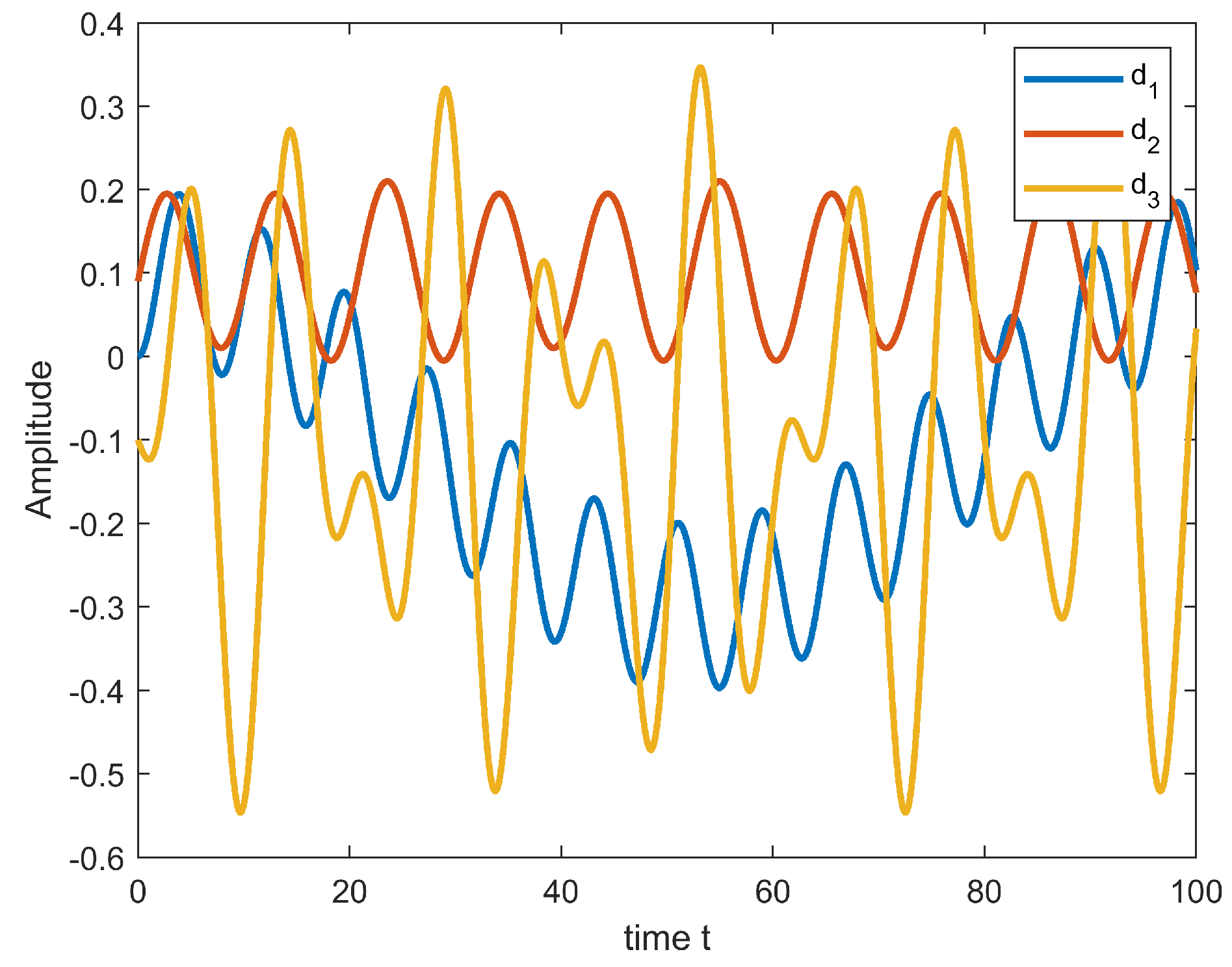
Initiating the system with χ ( 0 ) = [ 5 , 3 , 1 , 1 , 3 , 5 ] , the state responses of the closed-loop fuzzy system can be visualized in Figure 3. The illustrations emphasize the efficacy of the control design methodology, particularly in managing a stochastic Markovian process.
Remark 9. 
It should be pointed out that, in Figure 3, disturbances typically represent environmental influences, such as wind speed, pressure changes, and temperature variations, all of which can affect the performance and control of the aircraft system. In this paper, the disturbances we chose mainly serve to validate the effectiveness of the proposed method. The two sinusoidal waves can simulate periodic changes in wind speed, pressure, or temperature. It is worth noting that this paper does not consider the issue of disturbance amplitude, as the current disturbances are sufficient to demonstrate the advantages of our method. Additionally, actuator faults and disturbances are two different focus points in the system we consider, and their cumulative effects can impact the system’s robustness. Therefore, these disturbances are closely related to actuator faults, see Figure 1.

5. Conclusions

This study has addressed the significant challenge of implementing finite-time fault-tolerant control in nonlinear flexible spacecraft systems prone to random actuator faults. The approach is grounded on the T–S fuzzy model, where actuator malfunctions are represented as stochastic signals controlled by random Markov jumps. To adeptly navigate the intricacies brought about by these factors, we employ a depiction of the stochastic Markov process in the form of a polytope set. Our suggested approach entails the establishment of a sturdy stochastic Lyapunov stability structure, which is further augmented by the incorporation of adjustable parameters. Unlike the existing work [14], this work introduces a novel approach called GRCI, which maximizes the use of system information. This innovative controller design strategy culminates in a stability criterion that guarantees mean-square H performance. A numerical instance is illustrated to show the effectiveness and advantages of our suggested approach.

Author Contributions

Writing-original draft, W.X.; Writing-review & editing, Z.J.; Validation, Y.T. All authors have read and agreed to the published version of the manuscript.

Funding

This research was funded by the China Postdoctoral Science Foundation under Grant 2023M730411; the Chongqing postdoctoral innovativetalents support program under Grant CQBX202205; the Postdoctoral Fellowship Program of CPSF under GZB 20230913, GZC20241490.

Data Availability Statement

Data are contained within the article.

Conflicts of Interest

The authors declare no conflicts of interest.

References

  1. Dong, K.; Liu, H.; Zhu, X.; Wang, X.; Xu, F.; Liang, B. Force-free control for the flexible-joint robot in human-robot interaction. Comput. Electr. Eng. 2019, 73, 9–22. [Google Scholar] [CrossRef]
  2. Nath, K.; Bera, M.K. Event-triggered neuro sliding mode control for an uncertain Euler-Lagrange system: An impulsive dynamical system approach. Comput. Electr. Eng. 2022, 97, 107612. [Google Scholar] [CrossRef]
  3. Pradeep, C.; Eapen, M.E.; Joby, P.P.; Kizhakkethottam, J. Online placement and scheduling algorithm for reconfigurable cells in self-repairable field-programmable gate array systems. Comput. Electr. Eng. 2018, 67, 836–850. [Google Scholar]
  4. Mu, S.; Shibata, S.; Yamamoto, T.; Obayashi, H. Interface using eye-gaze and tablet input for an avatar robot control in class participation support system. Comput. Electr. Eng. 2023, 111, 108914. [Google Scholar] [CrossRef]
  5. Tian, Y.; Wang, Z. Stability analysis and generalized memory controller design for delayed T–S fuzzy systems via flexible polynomial-based functions. IEEE Trans. Fuzzy Syst. 2022, 30, 728–740. [Google Scholar] [CrossRef]
  6. Tian, Y.; Wang, Z. Finite-time extended dissipative filtering for singular T–S fuzzy systems with nonhomogeneous Markov jumps. IEEE Trans. Cybern. 2022, 52, 4574–4584. [Google Scholar]
  7. Li, A.; Liu, M.; Shi, Y. Adaptive sliding mode attitude tracking control for flexible spacecraft systems based on the Takagi–Sugeno fuzzy modelling method. Acta Astronaut. 2020, 175, 570–581. [Google Scholar] [CrossRef]
  8. Kumar, S.V.; Raja, R.; Anthoni, S.M.; Cao, J.; Tu, W. Robust finite-time non-fragile sampled-data control for T–S fuzzy flexible spacecraft model with stochastic actuator faults. Appl. Math. Comput. 2018, 321, 483–497. [Google Scholar]
  9. Cheng, J.; Park, J.; Wang, H. Event-triggered H control for T–S fuzzy nonlinear systems and its application to truck-trailer system. Appl. Math. Comput. 2016, 65, 62–71. [Google Scholar]
  10. Li, H.; Pan, Y.; Shi, P.; Shi, Y. Switched fuzzy output feedback control and its application to mass-spring-damping system. IEEE Trans. Fuzzy Syst. 2016, 24, 1259–1269. [Google Scholar] [CrossRef]
  11. Qiu, J.; Ding, S.; Gao, H.; Yin, S. Fuzzy-model-based reliable static output feedback H control of nonlinear hyperbolic PDE systems. IEEE Trans. Fuzzy Syst. 2016, 24, 388–400. [Google Scholar] [CrossRef]
  12. Dharani, S.; Rakkaiyappan, R.; Cao, J. Robust stochastic sampled-data H control for a class of mechanical systems with uncertainties. J. Dyn. Syst. Meas. Control. 2015, 137, 101008. [Google Scholar] [CrossRef]
  13. Sun, G.; Xu, S.; Li, Z. Finite-time fuzzy sampled-data control for nonlinear flexible spacecraft with stochastic actuator failure. IEEE Trans. Ind. Electron. 2017, 64, 3851–3861. [Google Scholar] [CrossRef]
  14. Xu, J.; Song, T.; Wang, J. Finite-time fuzzy fault-tolerant control for nonlinear flexible spacecraft system with stochastic actuator faults. Mathematics 2024, 12, 503. [Google Scholar] [CrossRef]
  15. Hu, S.; Yue, D.; Du, Z.; Liu, J. Reliable H non-uniform sampling tracking control for continuous-time non-linear systems with stochastic actuator faults. IET Control. Theory Appl. 2012, 6, 120–129. [Google Scholar] [CrossRef]
  16. Wang, C.; Zhang, H.; Yang, S.; Bo, C.; Li, J. Fuzzy-model-based finite-time control of nonlinear spacecrafts over a distributed sensor network. J. Frankl. Inst. 2023, 360, 2729–2750. [Google Scholar] [CrossRef]
  17. Wang, D.; Wu, F.; Lian, J.; Li, S. Observer-Based asynchronous control for stochastic nonhomogeneous semi-Markov jump systems. IEEE Trans. Autom. Control. 2023, 69, 2559–2566. [Google Scholar] [CrossRef]
  18. Golmakani, M.; Hubbard, R.; Miglioretti, D. Nonhomogeneous Markov chain for estimating the cumulative risk of multiple false positive screening tests. Biometrics 2022, 78, 1244–1256. [Google Scholar] [CrossRef] [PubMed]
  19. Tian, Y.; Su, X.; Shen, C.; Ma, X. Exponentially extended dissipativity-based filtering of switched neural networks. Automatica 2024, 161, 111465. [Google Scholar] [CrossRef]
  20. Tian, Y.; Wang, Z. Extended dissipativity analysis for Markovian jump neural networks via double-integral-based delay-product-type Lyapunov functiona. IEEE Trans. Neural Netw. Learn. Syst. 2021, 32, 3240–3246. [Google Scholar] [CrossRef]
  21. Xu, C.; Wu, B.; Wang, D.; Zhang, Y. Decentralized event-triggered finite-time attitude consensus control of multiple spacecraft under directed graph. J. Franklin Institute 2021, 358, 9794–9817. [Google Scholar] [CrossRef]
  22. Gao, S.; Liu, X.; Jing, J.; Dimirovski, G. A novel finite-time prescribed performance control scheme for spacecraft attitude tracking. Aerosp. Sci. Technol. 2021, 118, 107044. [Google Scholar] [CrossRef]
  23. Amrr, S.; Nabi, M. Finite-time fault tolerant attitude tracking control of spacecraft using robust nonlinear disturbance observer with anti-unwinding approach. Adv. Space Res. 2020, 66, 1659–1671. [Google Scholar] [CrossRef]
  24. Lee, D. Fault-tolerant finite-time controller for attitude tracking of rigid spacecraft using intermediate quaternion. IEEE Trans. Aerosp. Electron. Syst. 2020, 57, 540–553. [Google Scholar] [CrossRef]
  25. Zheng, C.; Cao, J.; Hu, M.; Fan, X. Finite-time stabilisation for discrete-time T–S fuzzy model system with channel fading and two types of parametric uncertainty. Int. J. Syst. Sci. 2017, 48, 34–42. [Google Scholar] [CrossRef]
  26. Gu, K. Stability of time-delay systems: Some recent advances. Automatica 2003, 39, 2099–2110. [Google Scholar]
  27. De la Sen, M. On the properties of reachability, observability, controllability, and constructibility of discrete-time positive time-invariant linear systems with aperiodic choice of the sampling instants. Discret. Dyn. Nat. Soc. 2007, 2007, 084913. [Google Scholar] [CrossRef]
  28. Troch, I. Sampling with arbitrary choice of the sampling instants. Automatica 1973, 9, 117–124. [Google Scholar] [CrossRef]
  29. Iandiorio, C.; Salvini, P. Elasto-kinematics and instantaneous invariants of compliant mechanisms based on flexure hinges. Micromachines 2023, 14, 783. [Google Scholar] [CrossRef]
Figure 1. Structure of the considered control system.
Symmetry 16 00873 g001
Figure 2. The disturbance of considered system.
Symmetry 16 00873 g002
Figure 3. The state responses of closed-loop control system.
Symmetry 16 00873 g003
Disclaimer/Publisher’s Note: The statements, opinions and data contained in all publications are solely those of the individual author(s) and contributor(s) and not of MDPI and/or the editor(s). MDPI and/or the editor(s) disclaim responsibility for any injury to people or property resulting from any ideas, methods, instructions or products referred to in the content.

