Improvement and Application of Hale’s Dynamic Time Warping Algorithm

Abstract

Due to the different generation and propagation mechanisms of P- and S-waves, there may be significant differences in the seismic data collected by the two, which poses a great obstacle to the time domain matching of P- and S-waves in multiwave exploration. Furthermore, the quality and accuracy of the matching effect will directly affect the subsequent multiwave joint inversion and interpretation effect. Therefore, the study of P and S-wave-matching methods plays a crucial role in seismic exploration. In 2013, Hale improved the classical Dynamic Time Warping (DTW) algorithm applied to solve the problem of speech recognition, and obtained the DTW algorithm suitable for solving the matching of P-waves and S-waves. The seismic wave-matching results generated by this algorithm are horizontal discontinuous (different trajectories) and need further processing. This study analyses the algorithm based on simulations of seismic waves using Ricker wavelets. In response to existing problems, this paper proposes strategies to improve the DTW algorithm. The algorithm in this study significantly improved the continuity of the registration results of the actual seismic wave data in the horizontal direction (different traces).

1. Introduction

Gaiser used the average velocity ratio $v_p/v_s$ of P-waves and S-waves to match P-waves and S-waves [1]. Chan used a new asymmetric shift-out correction (AMOC) technique to convert S-waves into pseudo P-waves for registration [2]. Dok and Gaiser used the principle of maximum similarity to scan the P-wave velocity ratio spectrum of seismic data in three blocks and selected the average P-wave velocity ratio to match the multiwaves in the time domain [3]. Baan and Kendall proposed a new fast method that uses the $\tau -\pi$ transform to accurately calculate the P- and S-wave reflection time-difference curves in layered, horizontally uniform, and anisotropic media [4]. Yuan used a simulated annealing algorithm to match P- and S-waves based on their maximum similarity objective function [5]. Garotta used the initial velocity ratio, simulated annealing method, and correlation method to update the P-wave and S-wave velocity ratios and complete the time-domain registration [6]. Deangelo conducted registration research of P-waves and S-waves in the depth domain and achieved a good practical application effect [7]. Fomel and Backus used the least-squares method to automatically match the time domains of the P- and S-waves, thereby reducing the interference of manually detecting the horizon. This method requires a suitable initial model to prevent the convergence result from falling into a local minimum [8]. Stewart et al. analysed the information obtained by conventional seismic exploration, mainly using compressional wave processing. Multicomponent seismic exploration uses both P- and S-waves to improve seismic imaging and to extract valuable additional information from underground physical parameters [9]. Liner and Clapp applied a nonlinear algorithm for P- and S-wave registration [10]. Nickel and Sonneland used P- and S-wave attributes for matching, calculated the P- and S-wave velocity ratios through multiple iterations, and then accurately matched the P- and S-waves in the time domain [11]. Fomel et al. first performed least-squares registration on the P-wave and S-wave data in the time domain; then, after registering the amplitudes and frequencies of the P- and S-waves, the remaining velocity ratio was scanned to update the time relationship between the P-wave and S-wave to complete the registration. This method can avoid the problem of local minima and has good adaptability to initial model errors. However, this method, which is based on the normalised cross-correlation between P-waves and S-waves, has certain requirements for the average velocity ratio of P-waves and S-waves [12]. Calvert et al. achieved a reasonable match when the similarity between P- and S-waves reached a maximum through the iterative calculation of the simulated annealing method, and also considered the influence of frequency band spectral whitening and phase correction [13]. Fomel and Jin introduced a method to match time-varying shifts in seismic data based on the local similarity of the two datasets [14]. Wang et al. applied a curve transformation to multicomponent seismic waves. The results showed that the registration result of this method was better than that of the mistie registration method, particularly in the case of significant noise. In addition, compared with previous single-scale registration methods, multiscale registration is less dependent on initial guesses [15]. Wang et al. proposed a one-norm minimization method to register the corresponding amplitudes of reflected events in P- and S-wave data [16]. Gao and Sacchi used the Gaussian-Newton method to calculate the regularisation function of the minimum cost function to realise P- and S-wave registrations [17]. Sarhan et al. proposed an image registration workflow that established a cost function to quantify the registration quality of images, and iteratively solved the optimisation problem until a registration image that met the requirements was obtained [18]. Mojtabazadeh-Hasanlouei et al. proposed a complete formula of the attenuated orthogonal time-domain half-space boundary element method for the analysis of the transient SH-wave scattering problem. A simple numerical model named DASBEM is successfully established by using the time-domain boundary element method (TD-BEM) based on the half-space Green function to analyse the heterogeneous orthogonal mountain topography [19,20,21].

Caparica and de Moraes used dynamic time warping (DTW) with initial speed and slope constraints for data registration [22]. Senin systematically summarised the application fields and theories of DTW [23]. Hale introduced time-varying shifts in the DTW method and applied them to P- and S-wave registrations [24]. Compton and Hale further expanded the DTW method to obtain multidimensional P- and S-wave registrations [25]. Venstad designed a regularisation method for the DTW algorithm to further improve its anti-noise performance [26]. Dhara and Bagaini developed a supervised machine learning problem based on optical flow estimation that can be solved using convolutional neural networks (CNNs), which achieved a higher accuracy than windowed cross-correlation (WCC) and dynamic image warping (DIW) [27].

Sakoe and Chiba added a slope constraint to the DP algorithm, avoiding the influence of the warping function and greatly improving the accuracy of the DP algorithm results [28]. Geler et al. compared Sakoe–Chiba global constraints and Itakura global constraints in neural networks [29]. Zhao proposes a structure-adaptive matching tracking method that combines DTW algorithm to estimate the similarity between adjacent seismic tracks and extract the optimal wavelet along the inclined plane. This structured implementation will significantly speed up the convergence of the decomposition process. The DTW algorithm is improved by combining the Euclidean distance of the seismic trace with the first time derivative of the seismic trace. Based on the principle of least squares, the amplitudes of all the extracted wavelets are updated synchronously, which improves the robustness and accuracy of seismic trace decomposition [30].

Hale proposed a DTW algorithm to achieve better registration results for one-dimensional S-waves after several iterations. However, for multidimensional S-waves, smoothness cannot be guaranteed in the horizontal direction, and overall, further processing is still required to obtain better registration results, such as two-sided smoothing, DIW, TSDP, etc. However, these methods require certain assumptions and reduce the accuracy of the registration results.

First, this study analyses the shortcomings of the path backtracking of Hale’s DTW algorithm using synthesised P-waves and S-waves obtained based on Ricker wavelets. Subsequently, an improvement strategy and improved DTW algorithm are proposed, and their effectiveness is verified using synthetic seismic wave data. Finally, actual seismic data are used to simulate and compare the matching results of the improved DTW algorithm and Hale’s DTW algorithm, which indicate that the improved DTW algorithm can obtain high-precision longitudinal and transverse wave-matching results only once, avoiding further processing, reducing time complexity, and improving matching efficiency.

2. DTW Algorithm

The DTW algorithm was first used in automatic speech recognition and is a classic algorithm for solving automatic speech recognition problems. The DTW algorithm can calculate the similarity between two time sequences, particularly for time sequences of different lengths and rhythms (such as audio sequences of the same word read by different people). The DTW algorithm warps the time sequence according to its characteristics (i.e., local scaling on the time axis) to make the morphology of the two sequences as consistent as possible and obtain the maximum possible similarity. In multiwave seismic exploration, the different conditions of anisotropy, geology, subsurface horizons, and other conditions mean that P-waves and S-waves are nonlinear transformation relationships, similar to the nonlinear registration of template sequence a (P-wave) and test sequence b (S-wave) for automatic speech recognition.Therefore, the DTW algorithm is suitable for solving the problems of P- and S-wave registration.

2.1. Principles of Algorithm

2.1.1. The Matching Process of DTW Algorithm

Suppose there are two sequences: template sequence $A=\left(a\right(1),a(2),\dots a(n\left)\right)$ and sequence $B=\left(b\right(1),b(2),\dots ,b(m\left)\right)$ to be matched.

1.

Alignment errors: The distance matrix $e(i,j)$ between different features is calculated based on the features of the two sequences, and the equation is as follows:

$$\begin{array}{c}\hfill e(i,j)={(a\left(i\right)-b\left(j\right))}^2,i=1,2,\dots ,n,j=1,2,\dots ,m\end{array}$$

Here, the alignment error e is an $n\times m$ matrix, $e(i,j)$ represents the distance between the i-th feature of the template sequence A and the j-th feature of the sequence B to be matched. The larger the difference between the two features, the larger the distance, and conversely, the smaller the distance. Note that the alignment error here can be changed to other non-negative functions; just make sure that each term of the alignment error e is non-negative.

2.

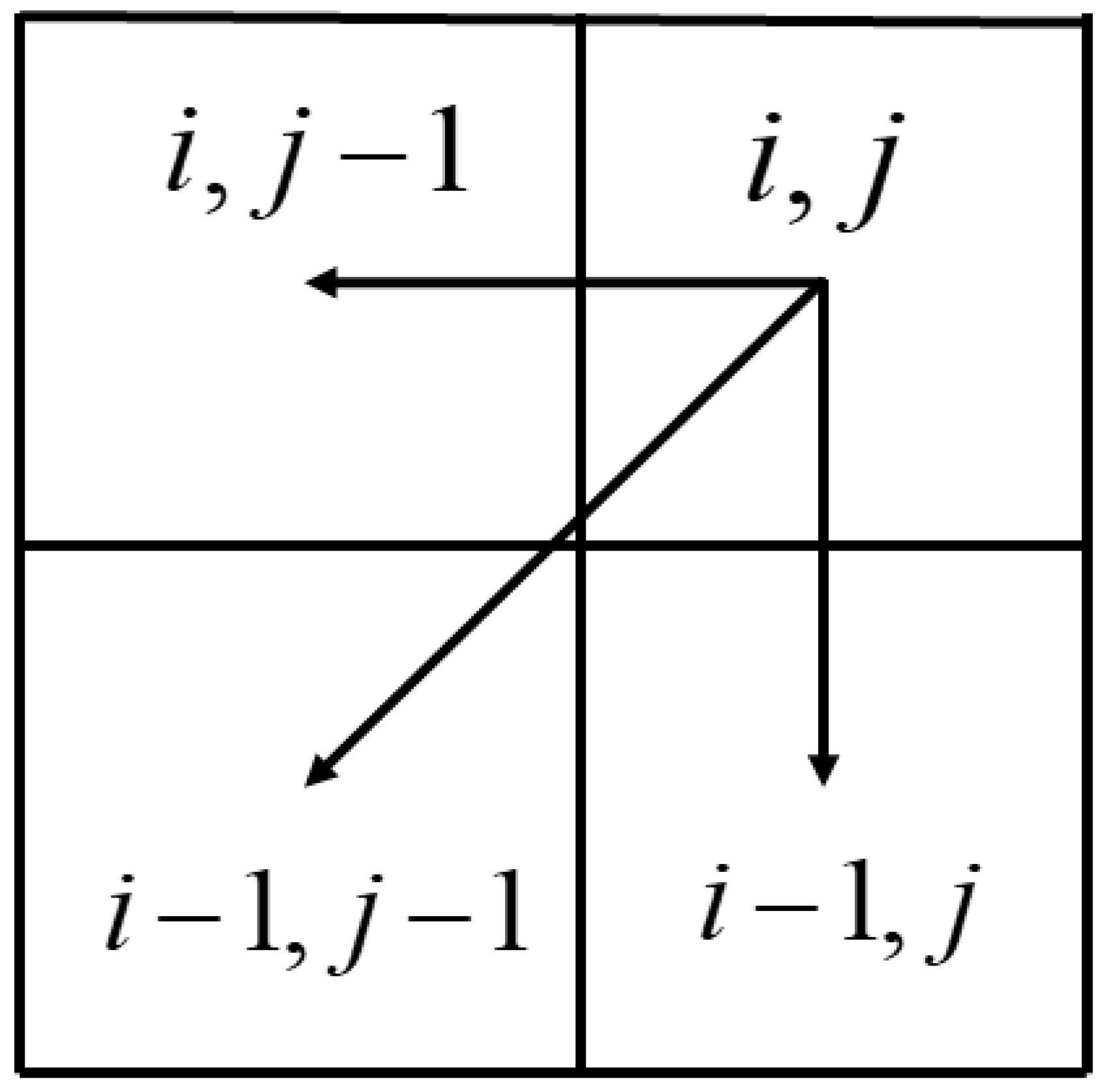
Accumulation: The global distance matrix $d(i,j)$ is obtained by recursive computation from the alignment error array $e(i,j)$, and the equation is as follows:

$$d(i,j)=min\left\{\begin{array}{c}d(i-1,j)+e(i,j),\hfill \\ d(i-1,j-1)+2e(i,j),\hfill \\ d(i,j-1)+e(i,j)\hfill \end{array}\right.j=2,3,\dots ,n,i=2,3,\dots ,n$$

Here, the accumulation d is an $n\times m$ matrix, the visualization of the formula process is shown in Figure 1, accumulation $d(i,j)$ is the minimum value obtained by summing the alignment errors $e(i,j)$ with $d(i-1,j)$, $d(i-1,j-1)$, and $d(i,j-1)$, respectively, where 2 is the weight coefficient, which is used to compensate for the displacement from $(i-1,j-1)$ to $(i,j)$ in the diagonal directions, and can be adjusted appropriately. The essential feature of the algorithm is to decompose a problem into a series of nested subproblems, so each $d(i,j)$ here is recorded as the minimum distance from the initial points $(1,1)$ to $(i,j)$, and similarly, d is the global minimum distance between the template sequence A and the sequence B to be matched.

3.

Backtracking: The path is obtained from the overall distance matrix inversion.

Through accumulation $d(n,m)$, the corresponding temporal relationship between the features of the template sequence A and sequence B to be matched can be inverted step by step, then the matching result can be obtained.

In the matching process, four constraints need to be satisfied: monotonicity, continuity, boundary conditions, and slope constraints.

2.1.2. Ricker Wavelet Principle

Mathematically, the Ricker wavelet is the second-order derivative of a Gaussian function that is symmetric in the time domain. In fact, they tend to be asymmetrical and are closer to the first-order derivative or the 1.5 derivative of a Gaussian function. However, the amplitude spectrum of the order derivatives of the Gaussian function are similar and obey a Gaussian distribution, so the Riker wavelet is often used in seismic analysis, for example, wave field simulation, reflection coefficient inversion, etc. The Ricker wavelet formula is

$$r\left(\tau \right)=(1-\frac{1}{2}{f}_p^2{\tau }^2)exp(-\frac{1}{4}{f}_p^2{\tau }^2)$$

where $\tau$ is the sampling interval, ms; $f_p$ is the centre frequency, Hz.

Figure 2a shows a synthetic P-wave based on the Ricker wavelet. $pp\left(i\right)$, $i=1,\dots ,n$, represents the P-wave amplitude, $n=396$ ms represents the sampling time. Figure 2b shows a synthetic S-wave based on the Ricker wavelet. $ps\left(i\right)$, $i=1,\dots ,m$, represents the S-wave amplitude and $m=396$ ms represents the sampling time length. Since S-waves propagate more slowly, it is realistic that the synthetic S-wave features are more backward compared to the synthetic P-wave, such that, for example, 250 ms for synthetic P-wave (a) actually corresponds approximately to 350 ms for synthetic S-wave (b). It can provide S-wave data for analysing the DTW algorithm.

2.2. Hale’s DTW Algorithm Analysis and Improvement Strategy

Figure 3a shows a synthetic P-wave based on the Ricker wavelet. $pp\left(i\right)$, $i=1,\dots ,n$, represents the P-wave amplitude, $n=396$ ms represents the sampling time. Figure 3b shows a synthetic S-wave based on the Ricker wavelet. $ps\left(i\right)$, $i=1,\dots ,m$, represents the S-wave amplitude and $m=396$ ms represents the sampling time length. Figure 3c represents the synthetic S-wave after registration using Hale’s DTW algorithm. Figure 3c, compared with Figure 3b, shows that the synthetic S-wave after registration loses data before 100 ms and after 300 ms of the synthetic S-wave. Figure 4 shows the time correspondence between the synthetic P- and S-waves after registration. The upper curve represents the synthetic P-wave, the lower curve represents the S-wave, and the connecting line represents the time correspondence between the synthetic P-wave and S-wave after registration. Figure 4 shows that the P-wave times corresponding to 130–150 ms and 235–250 ms of the synthetic S-wave times did not satisfy monotonicity in terms of the time sequence. Figure 5 shows the local time correspondence of 235–250 ms in Figure 4. From the orange solid line, it can be clearly observed that the time correspondence between the synthetic P-wave and synthetic S-wave is nonmonotonic; that is, there are cases of $(i,j)$ and $(i-1,j+1)$. In summary, Hale’s DTW algorithm has three problems with registration results:

1.

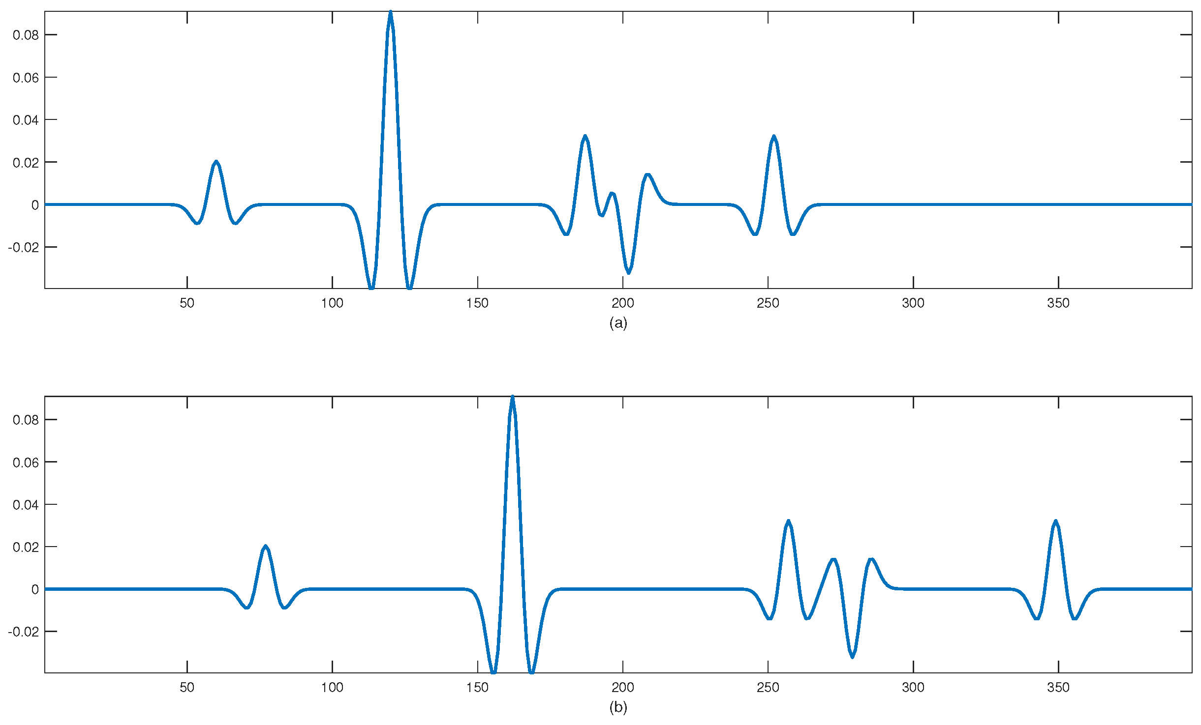
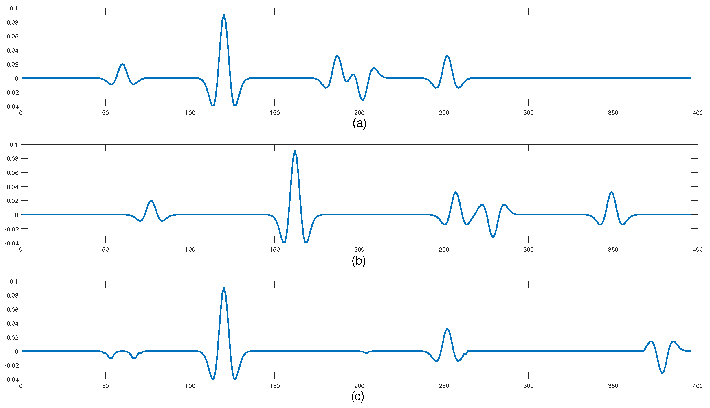
The synthetic S-wave lost some data after registration.

2.

The synthetic S-wave after registration and the synthetic P-wave were nonmonotonic in the corresponding time sequence.

3.

The synthetic S-wave after registration lost some of the data before the synthetic S-wave, which is similar to Problem 1, but for different reasons.

Supplementary concepts:

1.

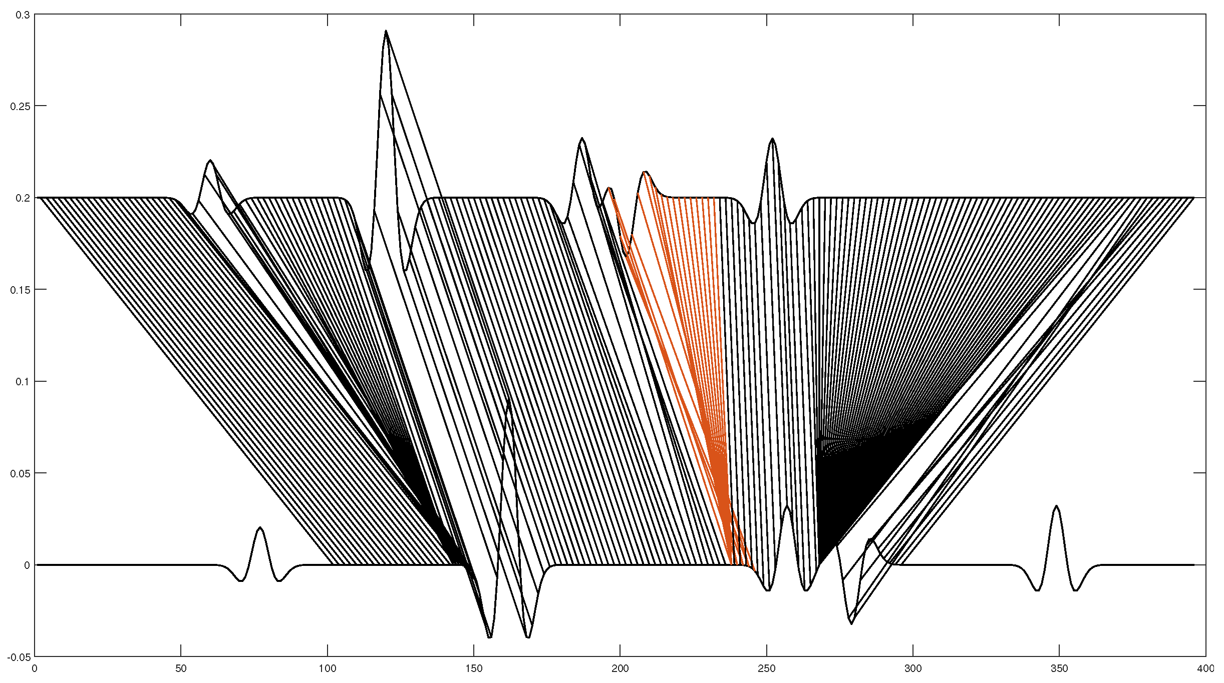
The time shift u is recorded in the S-wave after registration time point j corresponding to the P-wave time point i.

2.

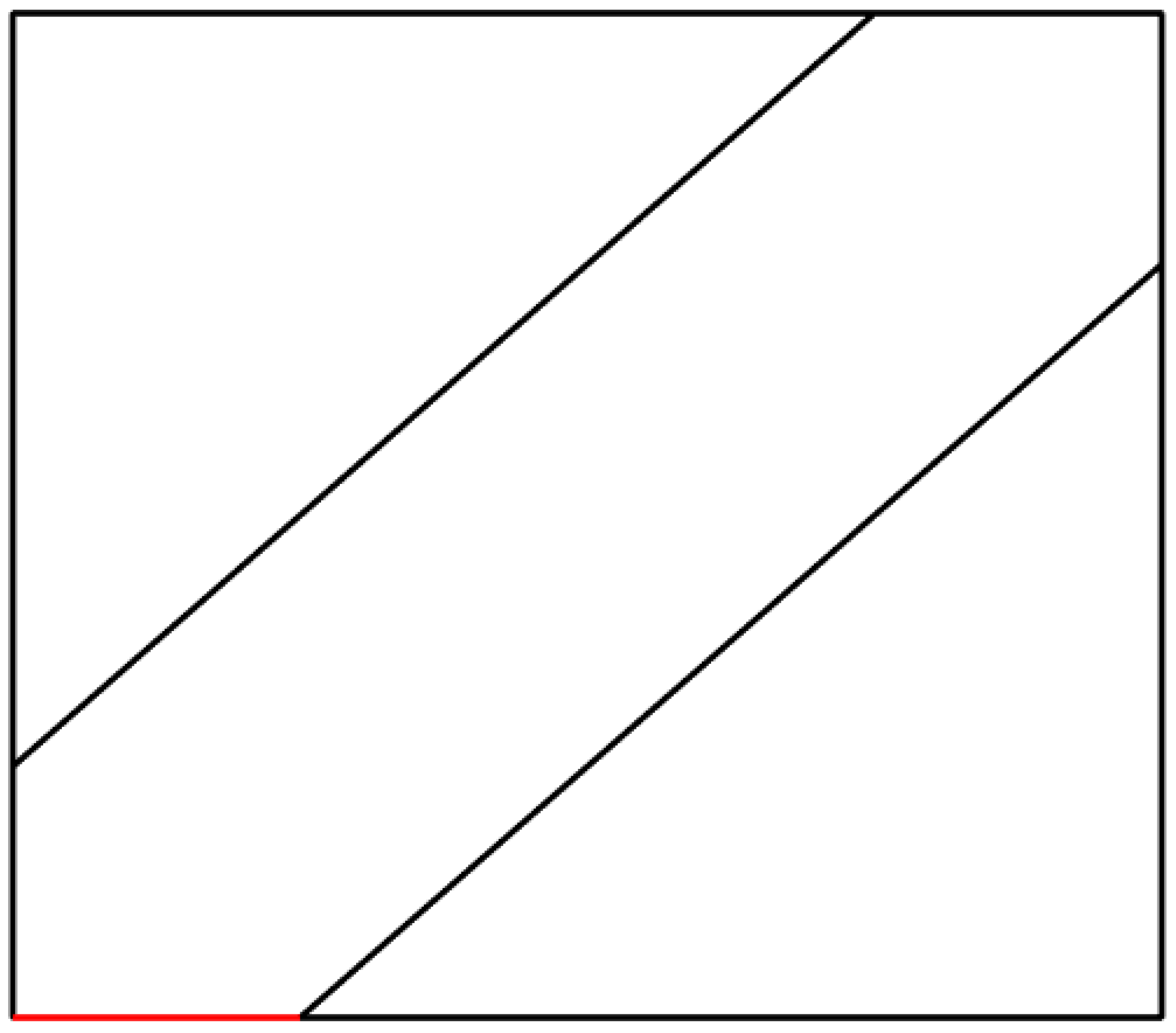
The slope constraint (Sakoe–Chiba constraint) can limit the registration range of P-wave and S-waves to quasi-diagonal, avoiding extreme situations. Assigning infinite values to areas outside the quasi-diagonal significantly reduces computational complexity and improves registration efficiency. L represents the range of slope constraints, which is the length of the red solid line in Figure 6. The P- and S-wave times between the two parallel lines satisfy $|i-j|<L$.

Next, we analyse the reasons for these three problems in detail, propose improvement strategies, and verify their feasibility using synthetic data.

Problem 1 is that the equation for the starting time shift $u\left(n\right)$ of Hale’s DTW algorithm path backtracking is

$$u\left(n\right)=arg\underset{j}{min}d(n,j)$$

That is, $u\left(n\right)$ takes the P-wave time point n corresponding to the S-wave time point j with the smallest accumulation within the slope constraint range ł. This may seem like an uncertain correspondence between the end times of the P- and S-waves, which to some extent dynamically selects the time points of the S-wave. However, when the end time of the P-wave corresponds to the end time of the S-wave or the effective duration of the S-wave is greater than the effective duration of the P-wave, some data on the time after the S-wave are lost, as shown in Figure 3c. The effective duration represents the time from time zero until the final amplitude is not zero (e.g., synthetic P-wave and synthetic S-wave).

Problem 2 occurs because the equation for the non-initial time shifts u of Hale’s DTW algorithm backtracking is

$$u\left(i\right)=\underset{j\in \left\{u\right(i+1)-1,u(i+1),u(i+1)+1\}}{argmin}d(i,j),i=n-1,n-2,\dots ,1$$

When $u\left(i\right)=u(i+1)+1$, the corresponding time sequences of $u\left(i\right)$ and $u(i+1)$ are nonmonotonic.

Problem 3 occurred because the initial amplitude of the P-wave was smaller than that of the S-wave. In Hale’s DTW algorithm backtracking, when $u\left(i\right)=u(i+1)-1$, the corresponding forward step size of the synthetic S-wave is 1, which is small. Therefore, at the P-wave time point $i=1$, the corresponding S-wave time point $j>1$ results in a loss of time before the S-wave.

Improvement strategy 1: Change the initial time shift $u\left(n\right)$ of the backtracking to

$$\begin{array}{c}\hfill u\left(n\right)=m\end{array}$$

(1)

$u\left(n\right)$ is equal to the last moment m of the S-wave; that is, the last time point n of the synthetic P-wave corresponds to the last time point m of the S-wave.

It should be noted that the P-wave time length n is not equal to the S-wave time length m. Because of the properties of an S-wave, m is typically greater than n. If m is approximately n, then zeros are added at the end of the P-wave. If there is a significant difference (by a factor of 1.5), it is necessary to compress the S-wave such that the S-wave time length m is equal to the P-wave time length n or slightly greater than the P-wave time length n and then add zero at the end of the P-wave.

Improvement strategy 2: Change $u(i+1)+1$ to $u(i+1)-2$ to avoid time sequence nonmonotonicity and increase the local step size. The equation for the non-initial time shift $u\left(i\right)$ of backtracking is

$$u\left(i\right)=\underset{j\in \left\{u\right(i+1)-2,u(i+1)-1,u(i+1\left)\right\}}{argmin}d(i,j),i=n-1,n-2,\dots ,1$$

Next, we verified the effect of $u(i+1)-2$.

The backtracking equation without $u(i+1)-2$.

$$u\left(n\right)=m$$

$$\begin{array}{c}\hfill u\left(i\right)=\underset{j\in \left\{u\right(i+1)-1,u(i+1\left)\right\}}{argmin}d(i,j),i=n-1,n-2,\dots ,1\end{array}$$

(2)

The accumulation equation corresponding to this backtracking is

$$d(1,j)=e(1,j),j=1,2,\dots ,m,$$

$$d(i,1)=e(i,1)+d(i-1,1),i=2,3,\dots ,n,$$

$$d(i,j)=e(i,j)+min\left\{\begin{array}{c}d(i-1,j-1),\hfill \\ d(i-1,j)\hfill \end{array}\right.,j=2,3,\dots ,n,i=2,3,\dots ,n$$

The backtracking equation with $u(i+1)-2$

$$u\left(n\right)=m$$

$$\begin{array}{c}\hfill u\left(i\right)=\underset{j\in \left\{u\right(i+1)-2,u(i+1)-1,u(i+1\left)\right\}}{argmin}d(i,j),i=n-1,n-2,\dots ,1\end{array}$$

(3)

The accumulation equation corresponding to this backtracking is

$$d(1,j)=e(1,j),j=1,2,\dots ,m,$$

$$d(i,1)=e(i,1)+d(i-1,1),i=2,3,\dots ,n,$$

$$d(i,2)=e(i,2)+min\left\{\begin{array}{c}d(i-1,1),\hfill \\ d(i-1,2)\hfill \end{array}\right.,i=2,3,\dots ,n$$

$$d(i,j)=e(i,j)+min\left\{\begin{array}{c}d(i-1,j-2),\hfill \\ d(i-1,j-1),\hfill \\ d(i-1,j)\hfill \end{array}\right.,j=3,4,\dots ,n,i=2,3,\dots ,n$$

Figure 7a shows a synthetic P-wave based on the Ricker wavelet. Figure 7b shows a synthetic S-wave based on the Ricker wavelet. Figure 7c shows the synthetic S-wave after registration using Equation (2). Figure 8 shows the time correspondence between the synthetic P- and S-waves after registration using Equation (2). Comparing Figure 7b and Figure 7c, it was found that the synthetic S-wave after registration did not lose data after 300 ms of the synthetic S-wave. In Figure 8, the time correspondence sequence between the synthetic P-wave and synthetic S-wave after registration with Equation (2) satisfies monotonicity, but the loss before 100 ms of data of the synthetic S-wave after registration still exists.

Figure 9a shows a synthetic P-wave based on the Ricker wavelet. Figure 9b shows a synthetic S-wave based on the Ricker wavelet. Figure 9c presents the synthetic S-wave after registration using Equation (3). Figure 10 shows the time correspondence between the synthetic P- and S-waves after registration using Equation (3). By comparing Figure 7c and Figure 9c, it was found that the registration results with Equation (3) were significantly better than those with Equation (2). In Figure 10, the amplitudes within the effective duration are preserved; thus, $u(i+1)-2$ has a good effect.

2.3. Improved DTW Algorithm

Based on the analysis and strategy of Hale’s DTW algorithm described in Section 2.2, an improved DTW algorithm was proposed. Suppose $pp$ is a P-wave with a sampling time of n, $pp\left(i\right),i=1,\dots ,n$. represents the P-wave amplitude, $ps$ is an S-wave with a sampling time of m, $ps\left(j\right),j=1$,…, and m. represents the S-wave amplitude. If $n\ne m$, the pre-processing method mentioned earlier must be used to process the S-wave. The improved DTW algorithm is as follows.

• Alignment Errors $e(i,j)$

$$\begin{array}{c}\hfill e(i,j)={(pp\left(i\right)-ps\left(j\right))}^2,i,j=1,2,\dots ,n\end{array}$$

(4)

• Accumulation $d(i,j)$

$$d(1,j)=e(1,j),j=1,2,\dots ,m,$$

$$d(i,1)=e(i,1)+d(i-1,1),i=2,3,\dots ,n,$$

$$d(i,2)=e(i,2)+min\left\{\begin{array}{c}d(i-1,1),\hfill \\ d(i-1,2)\hfill \end{array}\right.,i=2,3,\dots ,n$$

$$d(i,j)=e(i,j)+min\left\{\begin{array}{c}d(i-1,j-2),\hfill \\ d(i-1,j-1),\hfill \\ d(i-1,j)\hfill \end{array}\right.,j=3,4,\dots ,n,i=2,3,\dots ,n$$

(5)

Note here the range of shear wave time j, which needs to satisfy $j-1>0$ and $j-2>0$.

• Backtracking $s\left(i\right)$

$$u\left(n\right)=m$$

$$u\left(i\right)=\underset{j\in \left\{u\right(i+1)-2,u(i+1)-1,u(i+1\left)\right\}}{argmin}d(i,j),i=n-1,n-2,\dots ,1$$

$$\begin{array}{c}\hfill s\left(i\right)=ps\left(u\right(i\left)\right),i=1,2,\dots ,n\end{array}$$

(6)

3. Results and Discussion

The improved DTW algorithm was compared with Hale’s DTW algorithm using two field datasets.

From Figure 11, it can be seen that the DTW algorithm’s data matching results for any single-channel set of seismic data 1 still suffers from the three problems that occur in the synthetic data simulation. First, the S-wave still suffers from the first and the last data being discarded because the window width $L=36$ ms, and at most 72 ms (36 ms before and after) of the data can be discarded. Second, the problem of temporal nonmonotonicity still exists at 1600 ms and 1900 ms. Third, from the beginning of the path backtracking (2500 ms) when the time of the S-wave leads the time of the corresponding P-wave to the end of the path backtracking (0 ms) when the time of the S-wave lags behind the time of the corresponding P-wave, the gap between the time of the S-wave and that of the corresponding P-wave gradually increases throughout the path backtracking process, and it does not stop increasing until it is restricted by the constraint L. In conclusion, the simulation analysis based on synthetic data is accurate, not because of the particularity of synthetic data.

Field Data 1: The P-wave sampling time was 2501 ms, with a sampling interval of 1 ms, and the S-wave sampling time was 5001 ms, with a sampling interval of 1 ms. There were 1601 traces for both P- and S-waves.

Field Data 2: The P-wave sampling time was 2501 ms, with a sampling interval of 1 ms, and the S-wave sampling time was 5001 ms, with a sampling interval of 1 ms. There were 526 traces of P- and S-waves.

Because the sampling times of the P- and S-waves are different, it is necessary to pre-process the S-wave to obtain $m=n$. The equation used is as follows:

$$ps1\left(i\right)=max\left(ps\right(2i-1),ps(2i\left)\right),i=1,2,\dots ,2500$$

$$ps1\left(2501\right)=ps\left(5001\right)$$

An improved DTW algorithm such as Hale’s DTW method requires iterative processing of the S-wave of each trace for multidimensional shift registration.

Figure A1 presents a P-wave image from Data 1. Figure A2 shows an S-wave image from Data 1. Figure A3 shows the S-wave image after registration using Hale’s DTW algorithm within the range of the slope constraint $L=36$. Figure A4 shows the S-wave image after registration using the improved DTW algorithm within the range of slope constraint $L=36$. Figure A5 shows the estimated shift in Data 1 using Hale’s DTW algorithm. Figure A6 shows the estimated shift in Data 1 using the improved DTW algorithm.

Figure A7 shows the P-wave image of Data 2. Figure A8 shows an S-wave image from Data 2. Figure A9 shows the S-wave image after registration using Hale ’s DTW algorithm within the range of the slope constraint $L=200$. Figure A10 shows the S-wave image after registration using the improved DTW algorithm within the range of slope constraint $L=200$. Figure A11 shows the estimated shift in Data 1 using Hale’s DTW algorithm. Figure A12 shows the estimated shift in Data 1 using the improved DTW algorithm.

By comparing Figure A3 and Figure A4, as well as Figure A9 and Figure A10, the improved DTW algorithm can obtain clearer and smoother multidimensional S-wave registration results.

We find three problems in DTW algorithm through simulation. First, the selection of the initial path is unstable, resulting in the loss of the amplitude features of the later part of the shear wave. Second, the time is not monotonous, and the actual matching result is contradictory. Third, the backward step size is small, which will lose the amplitude characteristics of the time in front of the synthesised shear wave. In view of the existing problems, an improved strategy is proposed. The simulation verifies that the improved strategy is effective and there is no contradiction between the improved strategies, and the improved DTW algorithm is obtained by integrating the improved side rate. The improved DTW algorithm is generally applicable to the actual seismic data, and compared with the DTW algorithm, the similarity of matching results is greatly improved, and the X-axis direction is continuous. However, due to the increase in the backtracking step length, the matching result of the improved DTW algorithm is obviously discontinuous.

4. Conclusions

We find that the DTW algorithm has three problems in the simulation of single-channel integrated P-waves and synthetic S-waves. First, the selection of the initial path in the path backtracking results in the loss of amplitude features in the latter part of the synthetic S-wave. Second, the time order of the S-wave corresponding to the P-wave is not monotonic due to the selection of the non-starting path in path backtracking. Third, the amplitude features of the resultant S-wave front are lost due to the long and small advance of the resultant S-wave front in the path backtracking. The improved DTW algorithm is proposed to solve the three problems. Through the simulation and verification of synthetic P-wave and synthetic S-wave algorithms, the improved DTW algorithm solves the three problems, and the matching results are greatly improved to achieve the expected effect.

We still have three problems with the DTW algorithm in the measured seismic data, which are not caused by the difference between the synthetic data and the actual seismic data. Furthermore, the improved DTW algorithm is suitable for matching the measured seismic data of multi-channel sets. It shows that the improved DTW algorithm is universal and achieves higher similarity in the matching results of single and multi-channel sets.

Only the DTW and improved DTW methods are discussed here and effective matching results are obtained. In future work, we will improve the model and further quantify the matching results by adding constraints such as error analysis. Meanwhile, we would like to discuss the practicality of this problem by comparing more different matching methods.

References

1. Gaiser, J.E. Multicomponent vp/vs correlation analysis. Geophysics 1996, 61, 1137–1149. [Google Scholar] [CrossRef]
2. Chan, W. Analyzing Converted-Wave Seismic Data: Statics, Interpolation, Imaging, and p-p Correlation. Ph.D. Thesis, University of Calgary, Calgary, AB, Canada, 1998. [Google Scholar]
3. Dok, R.V.; Gaiser, J.E. Stratigraphic description of the morrow formation using mode-converted shear waves: Interpretation tools and techniques for three land surveys. Geophysics 2001, 61, 1042–1047. [Google Scholar]
4. Baan, M.V.D.; Kendall, J.M. Estimating anisotropy parameters and traveltimes in the r-p domain. Geophysics 2002, 67, 1076–1086. [Google Scholar] [CrossRef]
5. Yuan, J. Analysis of Four-Component Seafloor Seismic Data for Seismic Anisotrophy. Ph.D. Thesis, University of Edinburgh, Edinburgh, UK, 2001. [Google Scholar]
6. Garota, R.J. Acquisition/processing—Combined interpretation of pp and ps data provides direct access to elastic rock properties. Geophysics 2002, 21, 532–535. [Google Scholar]
7. Deangelo, M. Interpreters’ corner—Depth registration of p-wave and c-wave seismic data for shallow marine sediment characterization, gulf of mexico. Geophysics 2003, 22, 96–105. [Google Scholar]
8. Fomel, S.; Backus, M.M. Multicomponent seismic data registration by least squares. In SEG Technical Program Expanded Abstracts; SEG: Houston, TX, USA, 2003; Volume 22, pp. 781–784. [Google Scholar]
9. Stewart, R.R.; Gaiser, J.E.; Brown, R.J.; Lawton, D.C. Converted-wave seismic exploration: Applications. Geophysics 2003, 68, 40–57. [Google Scholar] [CrossRef]
10. Liner, C.L.; Clapp, R.G. Nonlinear pairwise alignment of seismic traces. Geophysics 2004, 69, 1552–1559. [Google Scholar] [CrossRef]
11. Nickel, M.A.; Sonneland, L. Automated ps to pp event regitration and estimation of a high-resolution vpvs ratio volume. In SEG Technical Program Expanded Abstracts; SEG: Houston, TX, USA, 2004; pp. 869–872. [Google Scholar]
12. Fomel, S.; Backus, M.M.; Fouad, K.; Hardage, B.A.; Winters, G. A multistep approach to multicomponent seismic image regitration with application to a west texas carbonate reservoir study. In SEG Technical Program Expanded Abstracts; SEG: Houston, TX, USA, 2005; pp. 1018–1021. [Google Scholar]
13. Calert, A.S.; Bloor, R.; Nathan, G.; Yuan, J. Automated C-wave registration by simulated annealing. In SEG Technical Program Expanded Abstracts; SEG: Houston, TX, USA, 2008; Volume 83, pp. 1043–1047. [Google Scholar]
14. Fomel, S.; Jin, L. Time-lapse image registration using the local similarity attribute. Geophysics 2009, 74, 2979–2983. [Google Scholar] [CrossRef]
15. Wang, H.; Cheng, Y.; Ma, J. Curvelet-based registration of multi-component seismic waves. Geophysics 2014, 104, 90–96. [Google Scholar] [CrossRef]
16. Wang, H.; Sacchi, M.D.; Ma, J. Linearized dynamic warping with ll-norm constraint for multi-component registration. Geophysics 2017, 139, 170–176. [Google Scholar]
17. Gao, W.; Sacchi, M.D. Multicomponent seismic data registration by nonlinear optimization. Geophysics 2018, 83, V1–V10. [Google Scholar] [CrossRef]
18. Sarhan, M.; Hathon, L.A.; Myers, M.; Arad, A. Development of multimodal/multidimensional image registration tools. In Proceedings of the SEG International Meeting for Applied Geoscience & Energy, Houston, TX, USA, 28 August–1 September 2022; pp. 2498–2501. [Google Scholar]
19. Mojtabazadeh-Hasanlouei, S.; Panji, M.; Kamalian, M. Attenuated orthotropic time-domain half-space BEM for SH-wave scattering problems. Geophys. J. Int. 2022, 229, 1881–1913. [Google Scholar] [CrossRef]
20. Mojtabazadeh-Hasanlouei, S.; Panji, M.; Kamalian, M. Scattering attenuation of transient SH-wave by an orthotropic gaussian-shaped sedimentary basin. Eng. Anal. Bound. Elem. 2022, 140, 186–219. [Google Scholar] [CrossRef]
21. Mojtabazadeh-Hasanlouei, S.; Panji, M.; Kamalian, M. A simple TD-BEM model for heterogeneous orthotropic hill-shaped topographies. Discov. Appl. Sci. 2024, 6, 57. [Google Scholar] [CrossRef]
22. Caparica, J.F.; de Moraes, F.S. On the use of dynamic time warping for multicomponent seismic data registration. In Proceedings of the 13th International Congress of the Brazilian Geophysical Society, Rio de Janeiro, Brazil, 26–29 August 2013. [Google Scholar]
23. Senin, P. Dynamic Time Warping Algorithm Review; Information and Computer Science Department University of Hawaii at Manoa: Honolulu, HI, USA, 2008; Volume 855, pp. 1–23. [Google Scholar]
24. Hale, D. Dynamic warping of seismic images. Geophysics 2013, 78, 105–115. [Google Scholar] [CrossRef]
25. Complon, S.; Hale, D. Estimating vp/vs ratios using smooth dynamic image warping. Geophysics 2014, 79, 201–215. [Google Scholar] [CrossRef]
26. Venstad, J.M. Dynamic time warping—An improved method for 4d and tomography time shift estimation. Geophysics 2014, 79, 209–220. [Google Scholar] [CrossRef]
27. Dhara, A.; Bagaini, C. Seismic image registration using multiscale convolutional neural networks. Geophysics 2020, 85, 425–441. [Google Scholar] [CrossRef]
28. Sakoe, H.; Chiba, S. Dynamic programming algorithm optimization for spoken word recognition. IEEE Trans. Acoust. Speech Signal Process. 1978, 26, 159–165. [Google Scholar] [CrossRef]
29. Geler, Z.; Kurbalia, V.; Ivanović, M.; Radovanović, M. Elastic distances for time-series classification: Itakura versus sakoe-chiba constraints. Knowl. Inf. Syst. 2022, 64, 2797–2832. [Google Scholar] [CrossRef]
30. Zhao, Z.; Rao, Y.; Wang, Y. Structure-adapted Multichannel Matching Pursuit for Seismic Trace Decomposition. Geophysics 2023, 180, 851–861. [Google Scholar] [CrossRef]
Figure 1. Schematic diagram of accumulation of the classic DTW algorithm.
Symmetry 16 00645 g001
Figure 2. (a) Synthetic P-wave based on the Ricker wavelet. (b) Synthetic S-wave based on the Ricker wavelet.
Symmetry 16 00645 g002
Figure 3. (a) Synthetic P-wave based on the Ricker wavelet. (b) Synthetic S-wave based on the Ricker wavelet. (c) Synthetic S-wave after registration with Hale’s DTW algorithm.
Symmetry 16 00645 g003
Figure 4. Time correspondence between the synthetic P-wave and the synthetic S-wave after registration.
Symmetry 16 00645 g004
Figure 5. At 235–250 ms in Figure 2, it can be seen that the local time sequence does not satisfy the monotonicity.
Symmetry 16 00645 g005
Figure 6. Sakoe–Chiba slope constraint.
Symmetry 16 00645 g006
Figure 7. (a) Synthetic P-wave based on the Ricker wavelet. (b) Synthetic S-wave based on the Ricker wavelet. (c) Synthetic S-wave after registration with Equation (2).
Symmetry 16 00645 g007
Figure 8. Time correspondence between the synthetic P-wave and the synthetic S-wave after registration with Equation (2).
Symmetry 16 00645 g008
Figure 9. (a) Synthetic P-wave based on the Ricker wavelet. (b) Synthetic S-wave based on the Ricker wavelet. (c) Synthetic S-wave after registration with Equation (3).
Symmetry 16 00645 g009
Figure 10. Time correspondence between the synthetic P-wave and the synthetic S-wave after registration with Equation (3).
Symmetry 16 00645 g010
Figure 11. (a) P-wave from Data 1. (b) S-wave from Data 1. (c) S-wave after registration with Hale’s DTW algorithm.
Symmetry 16 00645 g011
Disclaimer/Publisher’s Note: The statements, opinions and data contained in all publications are solely those of the individual author(s) and contributor(s) and not of MDPI and/or the editor(s). MDPI and/or the editor(s) disclaim responsibility for any injury to people or property resulting from any ideas, methods, instructions or products referred to in the content.