A New Three-Parameter Inverse Rayleigh Distribution: Simulation and Application to Real Data

Abstract

In this paper, we introduce a new three-parameter inverse Rayleigh distribution that extends the inverse Rayleigh distribution, constructed based on the generalized transmuted family of distributions proposed by Alizadeh, Merovci, and Hamedani. We explore statistical properties such as the quantile function, moments, harmonic mean, mean deviation, stress–strength reliability, and entropy. Parameter estimation is performed using various methods, including maximum likelihood, least squares, the method of the maximum product of spacings, and the method of Cramér–von Mises. The usefulness of the new three-parameter inverse Rayleigh distribution is illustrated by modeling a real dataset, demonstrating its superior fit compared to several other distributions.

1. Introduction

Initially, Treyer [1] introduced the inverse Rayleigh distribution as a model for analyzing reliability and survival data. The model later underwent further examination by Voda [2], who observed that the lifetime distributions of various experimental units could be closely approximated with the inverse Rayleigh distribution. Additionally, Voda explored its properties and provided a maximum likelihood (ML) estimator for the scale parameter.

Gharraph [3] conducted an in-depth analysis of the inverse Rayleigh distribution, deriving five key measures of location: the mean, harmonic mean, geometric mean, mode, and median. Furthermore, Gharraph explored various estimation methods to determine the unknown parameter of this distribution. A numerical comparison of these estimation techniques was conducted, focusing on their bias and root-mean-squared error (RMSE), providing valuable insights into their performance and applicability.

Mukherjee and Maiti [4] developed a percentile estimator for the scale parameter $\theta$ of one-parameter inverse Rayleigh distribution and investigated its asymptotic efficiency. Howlader et al. [5] established Bayesian prediction bounds for both Rayleigh and inverse Rayleigh lifetime models. Additionally, they demonstrated that the inverse Rayleigh (IR) model can serve as a viable alternative to the log-normal distribution for analyzing the survival time of specific diseases. Soliman et al. [6] addressed both Bayesian and non-Bayesian issues related to parameter estimation in the IR distribution.

Almarashi et al. [7] propose a two-parameter extension of the inverse Rayleigh distribution, employing the half-logistic transformation to address limitations in modeling moderately right-skewed or near-symmetrical lifetime data. Their theoretical contributions encompass mathematical properties and empirical evidence, demonstrating the model’s effectiveness in handling diverse right-skewed datasets.

Chiodo and Noia [8] present the inverse Rayleigh probability distribution as a robust model for estimating extreme wind speeds, crucial in wind power production and mechanical safety assessment. Their study not only validates the model’s capability in interpreting real wind speed data, but also introduces a novel Bayesian approach for estimating a dynamic “risk index”. Through extensive numerical simulations, they highlight the method’s precision and robustness, emphasizing its practical relevance for system engineers.

Furthermore, Chiodo et al. [9] introduce the compound inverse Rayleigh distribution as a model tailored for extreme wind speeds, essential in wind power generation and turbine safety evaluation. They provide a practical framework for real-world data analysis, accompanied by a novel Bayesian estimation approach, supported by extensive numerical simulations and robustness assessments.

In a different context, Bakoban and Al-Shehri [10] introduce the beta generalized inverse Rayleigh distribution, a four-parameter lifetime model, and conduct a comprehensive investigation into its properties and applications, further expanding the domain of inverse Rayleigh-based distributions.

Several generalizations of the inverse Rayleigh distribution have been recently proposed by numerous authors, with the aim of enhancing its adaptability. For example, Khan et al. [11] studied the modified inverse Rayleigh distribution and discussed its theoretical properties. Khan and King [12] enhanced the inverse Rayleigh distribution by proposing the transmuted modified inverse Rayleigh distribution, a new variant crafted through the utilization of the quadratic rank transmutation map (QRTM). Goual and Yousof [13] introduced an extension of the inverse Rayleigh distribution, termed the Burr XII inverse Rayleigh model, by integrating the Burr XII family framework initially introduced by Cordeiro et al. [14]. Ali [15] explored the use of the inverse Rayleigh distribution in mixture models to analyze the complex nature of engineering systems’ lifetimes. Drawing on the weighted distributions framework established by Fisher [16] and Rao [17], Fatima and Ahmad [18] introduced the Weighted Inverse Rayleigh (WIR) distribution. They conducted a comprehensive study of its statistical properties, contributing to the understanding and application of weighted distribution models in statistical analysis.

Rao and Mbwambo [19] developed the exponentiated inverse Rayleigh distribution (EIRD) to offer a more adaptable approach for life data analysis. This study examines its key statistical characteristics and assesses different estimation techniques such as the maximum likelihood and least squares. Banerjee and Bhunia [20] introduced the exponential transformed inverse Rayleigh distribution.

The generation of new distributions by adding one or more parameters to standard distributions enhances their applicability to complex data across various fields. Motivated by this approach, several authors have proposed different methods for generating new distributions. These include the Marshall–Olkin-G distribution [21], the Beta-G distribution introduced by Eugene et al. [22], the Kumaraswamy-G distribution by Cordeiro and Castro [23], and the McDonald-G distribution by Alexander et al. [24]. Shaw and Buckley [25] introduced the transmuted-G class of distributions, which was further expanded by the development of the exponentiated transmuted-G distribution [26] and the generalized transmuted G distribution [27].

Definition 1 

([27]). A random variable X is said to have a generalized transmuted-G distribution if its cumulative distribution function (CDF) is given by:

$$\begin{array}{c}\hfill F\left(x\right)=(1+\lambda )G{\left(x\right)}^{\alpha }-\lambda G{\left(x\right)}^{2\alpha },\alpha >0,-1\le \lambda \le 1,\end{array}$$

(1)

where $G\left(x\right)$ denotes the baseline cumulative distribution function.

The density function corresponding to this $\left(1\right)$ is given by

$$f\left(x\right)=\alpha g\left(x\right)G{\left(x\right)}^{\alpha -1}\left[1+\lambda -2\lambda G{\left(x\right)}^{\alpha }\right],$$

(2)

where $g\left(x\right)$ denotes the baseline probability density function.

Definition 2. 

A continuous random variable X is said to have an inverse Rayleigh distribution if its PDF is given by:

$$f(x;\sigma )=\frac{2{\sigma }^2}{x^3}{e}^{-{\left(\frac{\sigma }{x}\right)}^2},\mathit{for}x\ge 0\mathit{and}\sigma >0.$$

(3)

The CDF of the inverse Rayleigh distribution is given by:

$$F(x;\sigma )=e^{-{\left(\frac{\sigma }{x}\right)}^2},\mathrm{for}x\ge 0\mathrm{and}\sigma >0.$$

(4)

Substituting the PDF and CDF of the inverse Rayleigh distribution into Equations (1) and (2) results in the development of a new three-parameter inverse Rayleigh distribution, named the generalized transmuted inverse Rayleigh distribution.

Definition 3. 

A continuous random variable X is said to have a generalized transmuted inverse Rayleigh distribution (GTIR) if its PDF is given by:

$$f(x;\lambda ,\alpha ,\sigma )=\frac{2\alpha (1+\lambda ){\sigma }^2}{x^3}{e}^{-\alpha {\left(\frac{\sigma }{x}\right)}^2}-\frac{4\alpha \lambda {\sigma }^2}{x^3}{e}^{-2\alpha {\left(\frac{\sigma }{x}\right)}^2},$$

(5)

for $x\ge 0,\sigma >0,\alpha >0,$ and $\left|\lambda \right|\le 1.$

The cumulative distribution function of the generalized transmuted inverse Rayleigh distribution is given by:

$$F(x;\lambda ,\alpha ,\sigma )=\left(1+\lambda \right)e^{-\alpha {\left(\frac{\sigma }{x}\right)}^2}-\lambda e^{-2\alpha {\left(\frac{\sigma }{x}\right)}^2},$$

(6)

for $x\ge 0,\sigma >0,\alpha >0,$ and $\left|\lambda \right|\le 1.$

The hazard rate function (HRF) of the generalized transmuted inverse Rayleigh distribution is given by:

$$\begin{array}{cc}\hfill h(x;\lambda ,\alpha ,\sigma )& =\frac{f(x;\lambda ,\alpha ,\sigma )}{1-F(x;\lambda ,\alpha ,\sigma )}\hfill \\ \hfill & =\frac{\frac{2\alpha (1+\lambda ){\sigma }^2}{x^3}{e}^{-\alpha {\left(\frac{\sigma }{x}\right)}^2}-\frac{4\alpha \lambda {\sigma }^2}{x^3}{e}^{-2\alpha {\left(\frac{\sigma }{x}\right)}^2}}{1-\left(1+\lambda \right)e^{-\alpha {\left(\frac{\sigma }{x}\right)}^2}-\lambda e^{-2\alpha {\left(\frac{\sigma }{x}\right)}^2}}.\hfill \end{array}$$

(7)

Gupta [28] utilized the expression

$$\eta \left(x\right)=-\frac{f^{\prime }\left(x\right)}{f\left(x\right)},$$

to ascertain the monotonicity of the hazard function. Differentiating $f\left(x\right)$ with respect to x, we obtain:

$$\begin{array}{cc}\hfill \frac{\partial f\left(x\right)}{\partial x}& =\frac{-2\alpha {\sigma }^2}{x^6}exp\left(-\alpha \frac{{\sigma }^2}{x^2}\right)\hfill \\ \hfill & \times (8\alpha {\sigma }^{2}exp\left(-\alpha \frac{{\sigma }^2}{x^2}\right)\lambda -6exp\left(-\alpha \frac{{\sigma }^2}{x^2}\right)x^2\lambda \hfill \\ \hfill & -2\alpha \lambda {\sigma }^2-2\alpha {\sigma }^2+3\lambda x^2+3x^2).\hfill \end{array}$$

(8)

Now,

$$\begin{array}{cc}\hfill \eta \left(x\right)& =-\frac{f^{\prime }\left(x\right)}{f\left(x\right)}\hfill \\ \hfill & =-\frac{8\alpha \lambda {\sigma }^{2}exp\left(-\alpha \frac{{\sigma }^2}{x^2}\right)-6\lambda x^{2}exp\left(-\alpha \frac{{\sigma }^2}{x^2}\right)-2\alpha \lambda {\sigma }^2-2\alpha {\sigma }^2+3\lambda x^2+3x^2}{x^3\left(2\lambda exp\left(-\alpha \frac{{\sigma }^2}{x^2}\right)-\lambda -1\right)},\hfill \end{array}$$

(9)

$\eta \left(x\right)$ and $h\left(x\right)$ possess the same properties, and so, if $h\left(x\right)$ is unimodal, called an upside bathtub (UBT), we have ${\eta }^{\prime }\left(x\right)>0$ for $x\in (0,x_0)$, ${\eta }^{\prime }\left(x_0\right)=0$, and ${\eta }^{\prime }\left(x\right)<0$ for $x\in (x_0,\infty ),$ where $x_0$ can be obtained by solving the following equation:

$$\begin{array}{cc}\hfill 0=& \left(3{\lambda }^2+6\lambda +3\right)x_0^4+\left(-6\alpha {\sigma }^2{\lambda }^2-12\alpha {\sigma }^2\lambda -6\alpha {\sigma }^2\right)x_0^2{e}^{\frac{2\alpha {\sigma }^2}{x_0^2}}\hfill \\ \hfill & +\left(\left(-12{\lambda }^2-12\lambda \right)x_0^4+\left(36\alpha {\sigma }^2{\lambda }^2+36\alpha {\sigma }^2\lambda \right)x_0^2\right.\hfill \\ \hfill & \left.-8{\alpha }^2{\sigma }^4{\lambda }^2-8{\alpha }^2{\sigma }^4\lambda \right)e^{\frac{\alpha {\sigma }^2}{x_0^2}}+12{\lambda }^2{x}_0^4-48\alpha {\sigma }^2{\lambda }^2{x}_0^2.\hfill \end{array}$$

Solving this equation analytically would be quite complex due to its structure, involving both polynomial and exponential terms in $x_0$. Such equations usually do not have simple closed-form solutions and are typically approached with numerical methods for specific values of $\lambda$, $\alpha$, and $\sigma$.

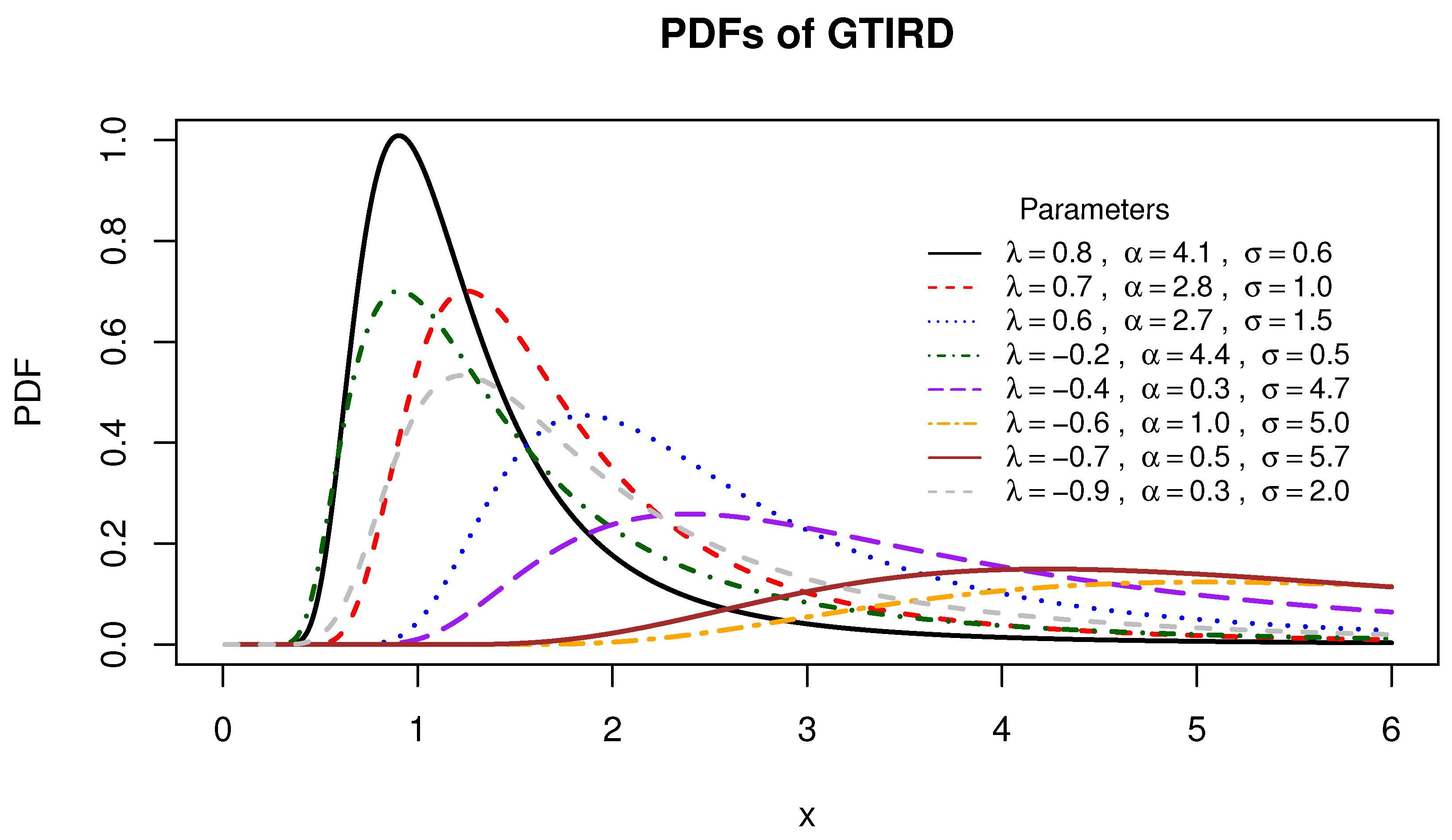
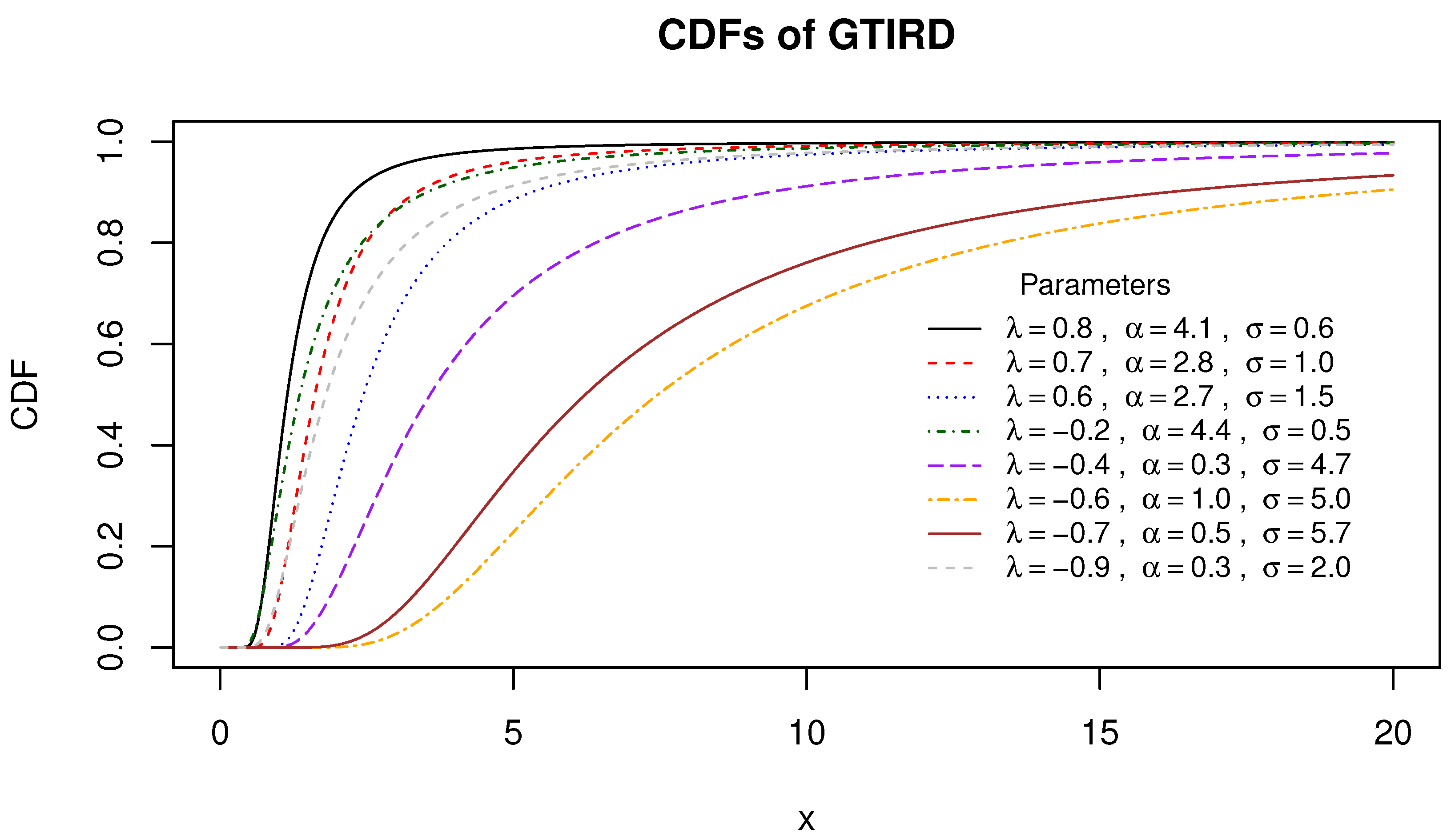
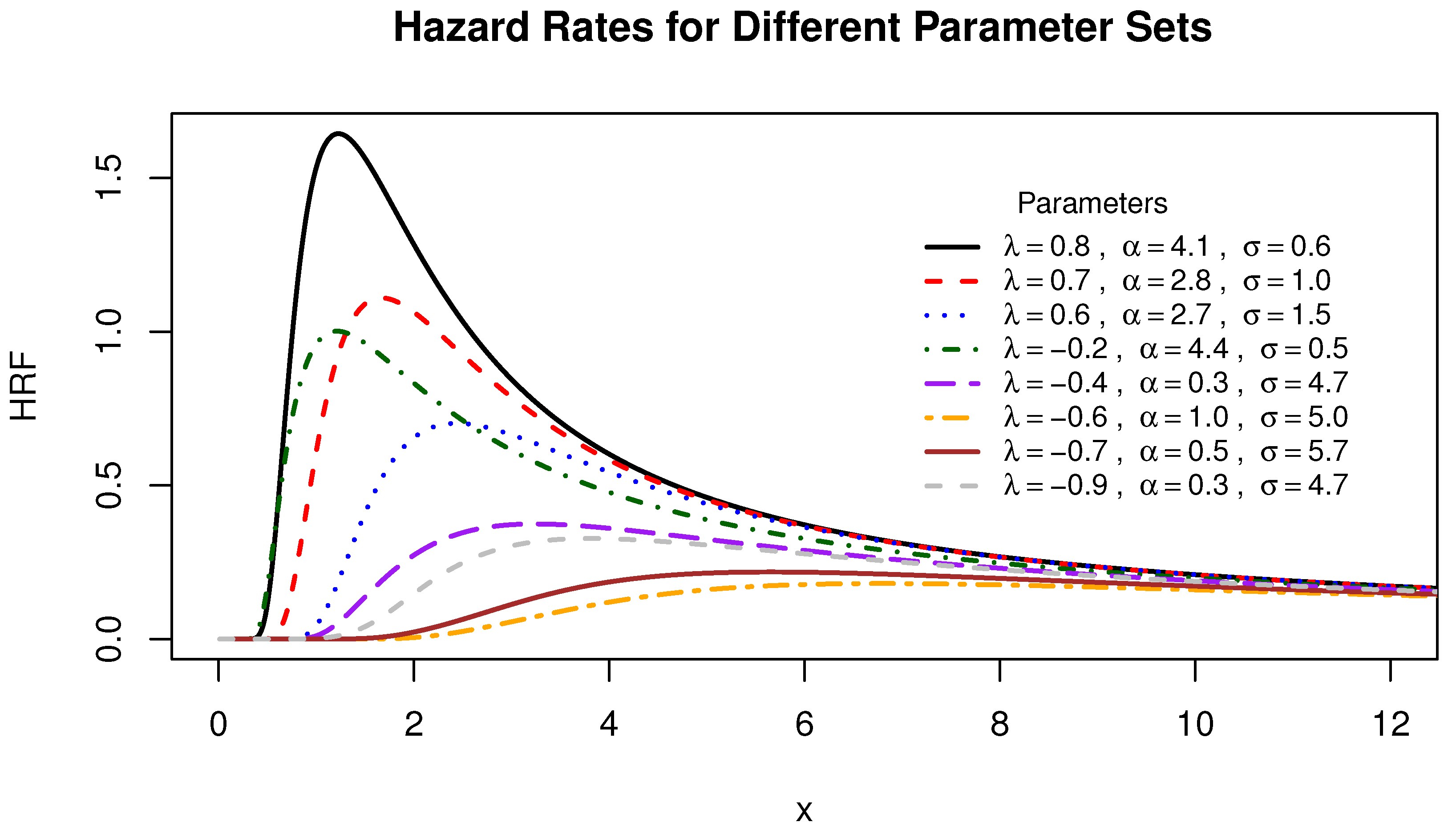
Figure 1, Figure 2 and Figure 3 illustrate the variability in the shapes of the PDF, CDF, and HRF for the generalized transmuted inverse Rayleigh distribution.

Figure 1 illustrates that the probability density function of the generalized transmuted inverse Rayleigh distribution displays shapes marked by decreasing, increasing, and unimodal patterns. From Figure 3, it is deduced that the hazard function of the generalized transmuted inverse Rayleigh distribution showcases a pattern characterized by decreasing, increasing, and unimodal shapes.

By varying the parameters, distinct distributions are obtained. For instance, when $\lambda =0$ and $\alpha =1$, the inverse Rayleigh distribution is attained. For $\alpha =1$ and $\left|\lambda \right|\le 1$, the transmuted inverse Rayleigh distribution is derived. Additionally, when $\lambda =-1$, the exponentiated inverse Rayleigh distribution with a shape parameter of $2\alpha$ is obtained.

2. Moments

Theorem 1. 

Let X be a random variable following a generalized transmuted inverse Rayleigh distribution with parameters $\lambda ,\alpha ,$ and $\sigma ,$ where λ is the transmutation parameter, α is the shape parameter, and σ is the scale parameter. The rth moment about the origin of X, denoted by $E\left(X^r\right)$, gives as:

$$E\left(X^r\right)={\alpha }^{\frac{r}{2}}{\sigma }^2\Gamma \left(1-\frac{r}{2}\right)\left[1+\lambda -2^{\frac{r}{2}}\lambda \right],r<2.$$

(10)

Proof. 

$$\begin{array}{cc}\hfill E\left(X^r\right)& ={\int }_0^{\infty }{x}^{r}f\left(x\right)dx={\int }_0^{\infty }{x}^r\left[\frac{2\alpha (1+\lambda ){\sigma }^2}{x^3}{e}^{-\alpha {\left(\frac{\sigma }{x}\right)}^2}-\frac{4\alpha \lambda {\sigma }^2}{x^3}{e}^{-2\alpha {\left(\frac{\sigma }{x}\right)}^2}\right]dx\hfill \\ \hfill & =2\alpha (1+\lambda ){\sigma }^2{\int }_0^{\infty }{x}^{r-3}{e}^{-\alpha {\left(\frac{\sigma }{x}\right)}^2}dx-4\alpha \lambda {\sigma }^2{\int }_0^{\infty }{x}^{r-3}{e}^{-2\alpha {\left(\frac{\sigma }{x}\right)}^2}dx\hfill \\ \hfill & =2\alpha (1+\lambda ){\sigma }^2{I}_1-4\alpha \lambda {\sigma }^2{I}_2.\hfill \end{array}$$

By using the integral formula

$${\int }_0^{\infty }{x}^{a-1}{e}^{-bx}dx=\frac{1}{b^a}\Gamma \left(a\right),$$

(11)

for $\Re \left(a\right)>0$ and $\Re \left(b\right)>0$ (see [29], p. 346), we have:

$$\begin{array}{cc}\hfill I_1& ={\int }_0^{\infty }{x}^{r-3}{e}^{-\alpha {\left(\frac{\sigma }{x}\right)}^2}dx\hfill \\ \hfill & =\left(\frac{1}{x^2}=t\Rightarrow x=\frac{1}{\sqrt{t}},dx=-\frac{1}{2}{t}^{-\frac{3}{2}}dt\right)\hfill \\ \hfill & =\frac{1}{2}{\int }_0^{\infty }{t}^{-\frac{r}{2}}{e}^{-\alpha {\sigma }^{2}t}dt=\frac{1}{2}{\int }_0^{\infty }{t}^{\left(1-\frac{r}{2}\right)-1}{e}^{-\alpha {\sigma }^{2}t}dt\hfill \\ \hfill & =\frac{1}{2{\left(\alpha {\sigma }^2\right)}^{1-\frac{r}{2}}}\Gamma \left(1-\frac{r}{2}\right),\hfill \end{array}$$

$$I_2={\int }_0^{\infty }{x}^{r-3}{e}^{-2\alpha {\left(\frac{\sigma }{x}\right)}^2}dx=\frac{1}{2{\left(2\alpha {\sigma }^2\right)}^{1-\frac{r}{2}}}\Gamma \left(1-\frac{r}{2}\right).$$

Now,

$$E\left(X^r\right)={\alpha }^{\frac{r}{2}}{\sigma }^2\Gamma \left(1-\frac{r}{2}\right)\left[1+\lambda -2^{\frac{r}{2}}\lambda \right],r<2.$$

   □

From Equation (10), it is evident that the generalized transmuted inverse Rayleigh distribution only possesses the first moment (mean). This indicates our ability to calculate the mean, but determining the variance and the higher order moments of this distribution is not possible. The mean of X is:

$$E\left(X\right)={\sigma }^2\sqrt{\pi \alpha }\left[1+\lambda -\sqrt{2}\lambda \right].$$

(12)

3. Harmonic Mean

Theorem 2. 

Let X be a random variable following a generalized transmuted inverse Rayleigh distribution with parameters λ, α, and σ. The harmonic mean (H) of X is given by:

$$H=\frac{\sqrt{\pi }}{2\sigma \sqrt{\alpha }}\left[1+\lambda -\frac{\sqrt{2}}{2}\lambda \right].$$

Proof. 

$$\begin{array}{cc}\hfill H& =E\left(\frac{1}{X}\right)\hfill \\ \hfill & ={\int }_0^{\infty }\frac{1}{x}f\left(x\right)dx\hfill \\ \hfill & ={\int }_0^{\infty }\frac{1}{x}\left[\frac{2\alpha (1+\lambda ){\sigma }^2}{x^3}{e}^{-\alpha {\left(\frac{\sigma }{x}\right)}^2}-\frac{4\alpha \lambda {\sigma }^2}{x^3}{e}^{-2\alpha {\left(\frac{\sigma }{x}\right)}^2}\right]dx\hfill \\ \hfill & =2\alpha (1+\lambda ){\sigma }^2{\int }_0^{\infty }{x}^{-4}{e}^{-\alpha {\left(\frac{\sigma }{x}\right)}^2}dx-4\alpha \lambda {\sigma }^2{\int }_0^{\infty }{x}^{-4}{e}^{-2\alpha {\left(\frac{\sigma }{x}\right)}^2}dx\hfill \\ \hfill & =\left.\left(\frac{1}{x^2}=t\Rightarrow x=\frac{1}{\sqrt{t}},dx=-\frac{1}{2}{t}^{-\frac{3}{2}}dt\right)\right|\hfill \\ \hfill & =\alpha (1+\lambda ){\sigma }^2{\int }_0^{\infty }{t}^{\frac{3}{2}-1}{e}^{-\alpha {\sigma }^{2}t}dt-2\alpha \lambda {\sigma }^2{\int }_0^{\infty }{t}^{\frac{3}{2}-1}{e}^{-2\alpha {\sigma }^{2}t}dt\hfill \\ \hfill & =\alpha (1+\lambda ){\sigma }^2\frac{1}{{\left(\alpha {\sigma }^2\right)}^{\frac{3}{2}}}\Gamma \left(\frac{3}{2}\right)-2\alpha \lambda {\sigma }^2\frac{1}{{\left(2\alpha {\sigma }^2\right)}^{\frac{3}{2}}}\Gamma \left(\frac{3}{2}\right)\hfill \\ \hfill & =\frac{\sqrt{\pi }}{2\sigma \sqrt{\alpha }}\left[1+\lambda -\frac{\sqrt{2}}{2}\lambda \right].\hfill \end{array}$$

   □

4. Quantile Function

In the study of probability distributions, the $\left(100p\right)$th percentile, denoted as ${\pi }_p$, where $0\le p\le 1$, is mathematically characterized by the value at which the cumulative distribution function (CDF), F, attains the probability p. This relationship is formalized by the equation:

$$F\left({\pi }_p\right)=P(X\le {\pi }_p)=p.$$

Theorem 3. 

The quantile function of the generalized transmuted inverse Rayleigh distribution, with parameters λ, α, and σ, is given by

$$x_p=Q\left(p\right)=\left\{\begin{array}{cc}\frac{-\alpha {\sigma }^2}{ln\left[\frac{1+\lambda -\sqrt{{(1+\lambda )}^2-4\lambda p}}{2\lambda }\right]}\hfill & \mathit{if}\lambda \ne 0,\hfill \\ \frac{\sigma }{\sqrt{-\frac{1}{\alpha }ln\left(p\right)}}\hfill & \mathit{if}\lambda =0.\hfill \end{array}\right.$$

(13)

Proof. 

Given the cumulative distribution function $F(x_p;\lambda ,\alpha ,\sigma )=p$, we start with the equation

$$\left(1+\lambda \right)e^{-\alpha {\left(\frac{\sigma }{x_p}\right)}^2}-\lambda e^{-2\alpha {\left(\frac{\sigma }{x_p}\right)}^2}=p.$$

(14)

For $\lambda \ne 0$, this equation simplifies to

$$\lambda e^{-2\alpha {\left(\frac{\sigma }{x_p}\right)}^2}-\left(1+\lambda \right)e^{-\alpha {\left(\frac{\sigma }{x_p}\right)}^2}+p=0.$$

By letting $e^{-\alpha {\left(\frac{\sigma }{x_p}\right)}^2}=t$, we obtain a quadratic equation in terms of t:

$$\lambda t^2-\left(1+\lambda \right)t+p=0.$$

Solving for t gives

$$t=\frac{1+\lambda -\sqrt{{(1+\lambda )}^2-4\lambda p}}{2\lambda }.$$

Substituting t back in terms of $x_p$, we obtain the quantile function as

$$x_p=Q\left(p\right)=\frac{-\alpha {\sigma }^2}{ln\left[\frac{1+\lambda -\sqrt{{(1+\lambda )}^2-4\lambda p}}{2\lambda }\right]}.$$

For $\lambda =0$, Equation (14) simplifies to

$$e^{-\alpha {\left(\frac{\sigma }{x_p}\right)}^2}=p,$$

which, upon rearrangement, yields the expression for $x_p$:

$$-\alpha {\left(\frac{\sigma }{x_p}\right)}^2=ln\left(p\right).$$

Solving for $x_p$, we obtain:

$$x_p=\frac{\sigma }{\sqrt{-\frac{1}{\alpha }ln\left(p\right)}}.$$

   □

Typically, the primary quartiles are identified as $Q_1$, signifying the 25th percentile with $Q_1=Q\left(0.25\right)$; $Q_2$, denoting the median or 50th percentile with $Q_2=Q\left(0.5\right)$; and $Q_3$, which corresponds to the 75th percentile with $Q_3=Q\left(0.75\right)$. These values are derived by setting the probabilities $p=0.25$, $p=0.5$, and $p=0.75$ into $X_p$. Furthermore, quartiles play a crucial role in determining the asymmetry and tail thickness of a distribution by aiding in the computation of its skewness and kurtosis.

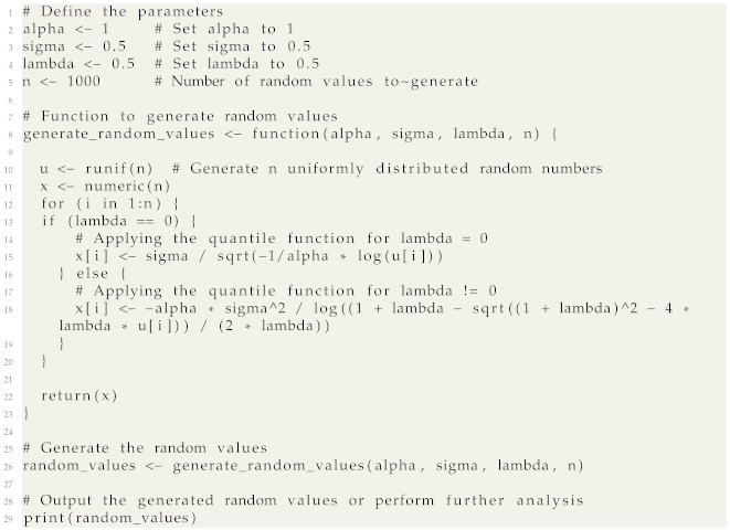
Assume a uniformly distributed variable U over the interval $(0,1)$, indicated as $U\sim \mathrm{Uniform}(0,1)$. Utilizing the equation referenced as (13), we can simulate a set of n random numbers consistent with a generalized transmuted inverse Rayleigh distribution. The formula to compute each random value $x_i$ is given by:

$$x_i=\left\{\begin{array}{cc}\frac{-\alpha {\sigma }^2}{ln\left[\frac{1+\lambda -\sqrt{{(1+\lambda )}^2-4\lambda u_i}}{2\lambda }\right]}\hfill & \mathrm{if}\lambda \ne 0,\hfill \\ \frac{\sigma }{\sqrt{-\frac{1}{\alpha }ln\left(u_i\right)}}\hfill & \mathrm{if}\lambda =0,\hfill \end{array}\right.$$

where i = 1, 2, 3, …, n.

5. R Code for Simulation Random Numbers from Generalized Transmuted Inverse Rayleigh Distribution

The following R script (Listing 1) demonstrates how to generate random values from the generalized transmuted inverse Rayleigh distribution:

Listing 1. R script for generating random values from the generalized transmuted inverse Rayleigh distribution.

6. Skewness and Kurtosis

Skewness is a statistical metric that captures the extent of asymmetry in a random variable’s probability distribution relative to the mean. A distribution may exhibit positive skewness, characterized by an elongated tail on the distribution’s right-hand side and a dense aggregation of data points on the left. Alternatively, a distribution may display negative skewness, which is denoted by a prolonged tail to the left and a denser accumulation of data on the right side of the distribution. The absence of skewness (zero value) signifies a symmetric distribution about the mean. However, there are instances when skewness cannot be determined. The coefficient of skewness using quartiles is expressed by the following equation:

$$\mathrm{Coefficient}\mathrm{of}\mathrm{Skewness}=\frac{Q_3-2Q_2+Q_1}{Q_3-Q_1},$$

where $Q_1$, $Q_2$, and $Q_3$ are the first, second (median), and third quartiles, respectively.

An alternative method for calculating kurtosis based on quantiles has been proposed by Moors [30]. This approach utilizes the following formula:

$$\mathrm{Kurtosis}=\frac{(E_7-E_5)+(E_3-E_1)}{(E_6-E_2)},$$

where $E_i$ is the ith octile, $E_i=F^{-1}(i/8).$

7. Mode

The mode of a continuous random variable with a probability density function $f\left(x\right)$ is the value at which $f\left(x\right)$ attains its maximum. Now, the mode of the generalized transmuted inverse Rayleigh distribution can be obtained by the solution of Equation (15):

$$\left.\begin{array}{cc}\hfill & \frac{\partial f}{\partial x}(x;\lambda ,\alpha ,\sigma )=0;\hfill \\ \hfill & \frac{{\partial }^{2}f}{\partial x^2}\left(x\right)<0;\hfill \\ \hfill & \frac{2\alpha {\sigma }^2{e}^{-\alpha {\left(\frac{\sigma }{x}\right)}^2}}{x^6}\left[(1+\lambda )(2\alpha {\sigma }^2-3x^2)+6\lambda x^2{e}^{-\alpha {\left(\frac{\sigma }{x}\right)}^2}-2\lambda e^{-\alpha {\left(\frac{\sigma }{x}\right)}^2}\right]=0.\hfill \end{array}\right\}$$

(15)

8. Mean Deviations

Deviation from the mean and median serves as a measure of the dispersion or scatter within a population. The collective deviations from both the mean and median contribute to what is referred to as the mean deviation about the mean and the mean deviation about the median. The mean Deviation about the mean is given by:

$${\delta }_1={\int }_0^{\infty }|x-\mu |f\left(x\right)dx=2\mu F\left(\mu \right)-2{\int }_0^{\mu }xf\left(x\right)dx$$

(16)

The mean deviation about the median is given by:

$${\delta }_2={\int }_0^{\infty }|x-m|f\left(x\right)dx=\mu -2{\int }_0^{m}xf\left(x\right)dx.$$

(17)

Theorem 4. 

The mean deviation about the mean and mean deviation about the median for the generalized transmuted inverse Rayleigh distribution are given by:

$$\begin{array}{cc}\hfill {\delta }_1& =2\mu F\left(\mu \right)-2\alpha (1+\lambda )\sigma ·\sqrt{\frac{\pi }{\alpha }}erfc\left(\frac{1}{\mu \sqrt{\frac{1}{\alpha {\sigma }^2}}}\right)\hfill \\ \hfill & +4\alpha \lambda \sigma ·\sqrt{\frac{\pi }{2}}\frac{1}{\sqrt{\alpha }}erfc\left(\frac{\sqrt{2}}{\mu \sqrt{\frac{1}{\alpha {\sigma }^2}}}\right),\hfill \end{array}$$

(18)

and

$$\begin{array}{cc}\hfill {\delta }_2=& \mu -2\alpha (1+\lambda )\sigma ·\sqrt{\frac{\pi }{\alpha }}erfc\left(\frac{1}{M\sqrt{\frac{1}{\alpha {\sigma }^2}}}\right)\hfill \\ \hfill & +4\alpha \lambda \sigma ·\sqrt{\frac{\pi }{2}}\frac{1}{\sqrt{\alpha }}erfc\left(\frac{\sqrt{2}}{M\sqrt{\frac{1}{\alpha {\sigma }^2}}}\right).\hfill \end{array}$$

(19)

Proof. 

$$\begin{array}{cc}\hfill {\int }_0^{\mu }xf\left(x\right)dx& ={\int }_0^{\mu }x\left[\frac{2\alpha (1+\lambda ){\sigma }^2}{x^3}{e}^{-\alpha {\left(\frac{\sigma }{x}\right)}^2}-\frac{4\alpha \lambda {\sigma }^2}{x^3}{e}^{-2\alpha {\left(\frac{\sigma }{x}\right)}^2}\right]dx\hfill \\ \hfill & =2\alpha (1+\lambda ){\sigma }^2{\int }_0^{\mu }\frac{1}{x^2}{e}^{-\alpha {\left(\frac{\sigma }{x}\right)}^2}dx-4\alpha \lambda {\sigma }^2{\int }_0^{\mu }\frac{1}{x^2}{e}^{-2\alpha {\left(\frac{\sigma }{x}\right)}^2}dx\hfill \\ \hfill & =\alpha (1+\lambda )\sigma ·\sqrt{\frac{\pi }{\alpha }}erfc\left(\frac{1}{\mu \sqrt{\frac{1}{\alpha {\sigma }^2}}}\right)\hfill \\ \hfill & -2\alpha \lambda \sigma ·\sqrt{\frac{\pi }{2}}\frac{1}{\sqrt{\alpha }}erfc\left(\frac{\sqrt{2}}{\mu \sqrt{\frac{1}{\alpha {\sigma }^2}}}\right).\hfill \end{array}$$

(20)

By substituting the expression from (20) into both (16) and (17), the mean deviations are obtained. □

9. Entropy

Two popular entropy measures are the Shannon entropy and its generalization, known as the Rényi entropy [31,32]. The Shannon entropy for GTIR distribution is given by:

$$\begin{array}{cc}\hfill H\left(X\right)& =-{\int }_0^{\infty }f\left(x\right)log\left[\alpha g\left(x\right)G{\left(x\right)}^{\alpha -1}\left(1+\lambda -2\lambda G{\left(x\right)}^{\alpha }\right)\right]dx\hfill \\ \hfill & =-{\int }_0^{\infty }f\left(x\right)\left[log\left(\alpha \right)+log\left(g\left(x\right)\right)+(\alpha -1)log\left(G\left(x\right)\right)+log\left(1+\lambda -2\lambda G{\left(x\right)}^{\alpha }\right)\right]dx\hfill \\ \hfill & =-log\left(\alpha \right)-{\int }_0^{\infty }f\left(x\right)log\left(g\left(x\right)\right)dx\hfill \\ \hfill & -(\alpha -1){\int }_0^{\infty }f\left(x\right)log\left(G\left(x\right)\right)dx\hfill \\ \hfill & -{\int }_0^{\infty }f\left(x\right)log\left[1+\lambda -2\lambda G{\left(x\right)}^{\alpha }\right]dx\hfill \\ \hfill & =-log\left(2\alpha {\sigma }^2\right)+3{\int }_0^{\infty }f\left(x\right)log\left(x\right)dx\hfill \\ \hfill & +(2\alpha -1){\sigma }^2{\int }_0^{\infty }\frac{1}{x^2}f\left(x\right)dx\hfill \\ \hfill & -{\int }_0^{\infty }f\left(x\right)log\left[1+\lambda -2\lambda e^{-\alpha {\left(\frac{\sigma }{x}\right)}^2}\right]dx\hfill \\ \hfill & =-log\left(2\alpha {\sigma }^2\right)+3{\int }_0^{\infty }\left[\frac{2\alpha (1+\lambda ){\sigma }^2}{x^3}{e}^{-\alpha {\left(\frac{\sigma }{x}\right)}^2}-\frac{4\alpha \lambda {\sigma }^2}{x^3}{e}^{-2\alpha {\left(\frac{\sigma }{x}\right)}^2}\right]log\left(x\right)dx\hfill \\ \hfill & +(2\alpha -1){\sigma }^2{\int }_0^{\infty }\frac{1}{x^2}\left[\frac{2\alpha (1+\lambda ){\sigma }^2}{x^3}{e}^{-\alpha {\left(\frac{\sigma }{x}\right)}^2}-\frac{4\alpha \lambda {\sigma }^2}{x^3}{e}^{-2\alpha {\left(\frac{\sigma }{x}\right)}^2}\right]dx\hfill \\ \hfill & -{\int }_0^{\infty }\left[\frac{2\alpha (1+\lambda ){\sigma }^2}{x^3}{e}^{-\alpha {\left(\frac{\sigma }{x}\right)}^2}-\frac{4\alpha \lambda {\sigma }^2}{x^3}{e}^{-2\alpha {\left(\frac{\sigma }{x}\right)}^2}\right]log\left[1+\lambda -2\lambda e^{-\alpha {\left(\frac{\sigma }{x}\right)}^2}\right]dx.\hfill \end{array}$$

(21)

The above integrals cannot be solved directly through analytical methods. Therefore, we use some numerical techniques to solve the integrals.

10. Stress–Strength Reliability

The stress–strength reliability, often represented in the context of engineering and reliability analysis, is a measure used to predict the reliability or performance of a system under operational conditions. It is based on the comparison between the distribution of stress (representing the demands or loads placed on the system) and the distribution of strength (representing the system’s ability to withstand those demands) over a certain period of time or under specific conditions.

Mathematically, stress–strength reliability can be denoted as $R=P(Strength>Stress)$, which means it is the probability that the strength of a component or system exceeds the stress applied to it during its operational life. This probability is crucial for designing components and systems that are expected to perform reliably under a range of operational conditions and for predicting their lifespan or the likelihood of failure. The stress–strength reliability is defined by the following.

Theorem 5. 

Let the strength of a system be $X\sim GTIR(x;{\lambda }_1,{\alpha }_1,{\sigma }_1)$ and the stress $Y\sim GTIR(y;{\lambda }_2,{\alpha }_2,{\sigma }_2)$. The reliability under the GTIR stress–strength model is given by:

$$\begin{array}{cc}\hfill R& =\frac{{\alpha }_1(1+{\lambda }_1)(1+{\lambda }_2){\sigma }_1^2}{{\alpha }_1{\sigma }_1^2+{\alpha }_2{\sigma }_2^2}-\frac{2{\alpha }_1{\lambda }_1(1+{\lambda }_2){\sigma }_1^2}{2{\alpha }_1{\sigma }_1^2+{\alpha }_2{\sigma }_2^2}\hfill \\ \hfill & -\frac{2{\alpha }_1(1+{\lambda }_1){\lambda }_2{\sigma }_1^2}{{\alpha }_1{\sigma }_1^2+2{\alpha }_2{\sigma }_2^2}+\frac{2{\alpha }_1{\lambda }_1{\lambda }_2{\sigma }_1^2}{2{\alpha }_1{\sigma }_1^2+2{\alpha }_2{\sigma }_2^2}.\hfill \end{array}$$

(22)

Proof. 

$$\begin{array}{cc}\hfill R& ={\int }_0^{\infty }\left\{{\int }_0^x{f}_Y(y;{\lambda }_2,{\alpha }_2,{\sigma }_2)dy\right\}{f}_X(x;{\lambda }_1,{\alpha }_1,{\sigma }_1)dx\hfill \\ \hfill & ={\int }_0^{\infty }{f}_X(x;{\lambda }_1,{\alpha }_1,{\sigma }_1)F_Y(x;{\lambda }_2,{\alpha }_2,{\sigma }_2)dx\hfill \\ \hfill & ={\int }_0^{\infty }\left[\frac{2{\alpha }_1(1+{\lambda }_1){\sigma }_1^2}{x^3}{e}^{-{\alpha }_1{\left(\frac{{\sigma }_1}{x}\right)}^2}-\frac{4{\alpha }_1{\lambda }_1{\sigma }_1^2}{x^3}{e}^{-2{\alpha }_1{\left(\frac{{\sigma }_1}{x}\right)}^2}\right]\hfill \\ \hfill & \times \left[\left(1+{\lambda }_2\right)e^{-{\alpha }_2{\left(\frac{{\sigma }_2}{x}\right)}^2}-{\lambda }_2{e}^{-2{\alpha }_2{\left(\frac{{\sigma }_2}{x}\right)}^2}\right]dx\hfill \\ \hfill & ={\int }_0^{\infty }\frac{2{\alpha }_1(1+{\lambda }_1)(1+{\lambda }_2){\sigma }_1^2}{x^3}{e}^{-\left(\frac{{\alpha }_1{\sigma }_1^2+{\alpha }_2{\sigma }_2^2}{x^2}\right)}dx\hfill \\ \hfill & -{\int }_0^{\infty }\frac{4{\alpha }_1{\lambda }_1(1+{\lambda }_2){\sigma }_1^2}{x^3}{e}^{-\left(\frac{2{\alpha }_1{\sigma }_1^2+{\alpha }_2{\sigma }_2^2}{x^2}\right)}dx\hfill \\ \hfill & -{\int }_0^{\infty }\frac{2{\alpha }_1(1+{\lambda }_1){\lambda }_2{\sigma }_1^2}{x^3}{e}^{-\left(\frac{{\alpha }_1{\sigma }_1^2+2{\alpha }_2{\sigma }_2^2}{x^2}\right)}dx\hfill \\ \hfill & +{\int }_0^{\infty }\frac{4{\alpha }_1{\lambda }_1{\lambda }_2{\sigma }_1^2}{x^3}{e}^{-\left(\frac{2{\alpha }_1{\sigma }_1^2+2{\alpha }_2{\sigma }_2^2}{x^2}\right)}dx.\hfill \\ \hfill & \left(\frac{1}{x^2}=t\Rightarrow ,dx=-\frac{1}{2}{t}^{-\frac{3}{2}}dt,1/x^3=t^{\frac{3}{2}}\right)\hfill \\ \hfill & ={\alpha }_1(1+{\lambda }_1)(1+{\lambda }_2){\sigma }_1^2{\int }_0^{\infty }{e}^{-\left({\alpha }_1{\sigma }_1^2+{\alpha }_2{\sigma }_2^2\right)t}dt\hfill \\ \hfill & -2{\alpha }_1{\lambda }_1(1+{\lambda }_2){\sigma }_1^2{\int }_0^{\infty }{e}^{-\left(2{\alpha }_1{\sigma }_1^2+{\alpha }_2{\sigma }_2^2\right)t}dt\hfill \\ \hfill & -2{\alpha }_1(1+{\lambda }_1){\lambda }_2{\sigma }_1^2{\int }_0^{\infty }{e}^{-\left({\alpha }_1{\sigma }_1^2+2{\alpha }_2{\sigma }_2^2\right)t}dt\hfill \\ \hfill & +2{\alpha }_1{\lambda }_1{\lambda }_2{\sigma }_1^2{\int }_0^{\infty }{e}^{-\left(2{\alpha }_1{\sigma }_1^2+2{\alpha }_2{\sigma }_2^2\right)t}dt.\hfill \\ \hfill & =\frac{{\alpha }_1(1+{\lambda }_1)(1+{\lambda }_2){\sigma }_1^2}{{\alpha }_1{\sigma }_1^2+{\alpha }_2{\sigma }_2^2}-\frac{2{\alpha }_1{\lambda }_1(1+{\lambda }_2){\sigma }_1^2}{2{\alpha }_1{\sigma }_1^2+{\alpha }_2{\sigma }_2^2}\hfill \\ \hfill & -\frac{2{\alpha }_1(1+{\lambda }_1){\lambda }_2{\sigma }_1^2}{{\alpha }_1{\sigma }_1^2+2{\alpha }_2{\sigma }_2^2}+\frac{2{\alpha }_1{\lambda }_1{\lambda }_2{\sigma }_1^2}{2{\alpha }_1{\sigma }_1^2+2{\alpha }_2{\sigma }_2^2}.\hfill \end{array}$$

□

11. Order Statistics

Consider $X_1,X_2,\dots ,X_n$, a set of continuous random variables that are independent and identically distributed (iid). Each variable has a probability density function denoted as $f\left(x\right)$ and a cumulative distribution function represented by $F\left(x\right)$. The probability density function for the kth smallest value among these random variables, known as the kth order statistic $X_{\left(k\right)}$, can be expressed as follows:

$$f_{X_{\left(k\right)}}\left(x\right)=\frac{n!}{(k-1)!(n-k)!}{f}_X\left(x\right){\left[F_X\left(x\right)\right]}^{k-1}{\left[1-F_X\left(x\right)\right]}^{n-k},$$

where k indexes from 1 to n.

The pdf of the kth order statistic for a generalized transmuted inverse Rayleigh distribution is given by:

$$\begin{array}{cc}\hfill f_{X_{\left(k\right)}}\left(x\right)=& \frac{n!}{(k-1)!(n-k)!}\left[\frac{2\alpha (1+\lambda ){\sigma }^2}{x^3}{e}^{-\alpha {\left(\frac{\sigma }{x}\right)}^2}-\frac{4\alpha \lambda {\sigma }^2}{x^3}{e}^{-2\alpha {\left(\frac{\sigma }{x}\right)}^2}\right]\hfill \\ \hfill & \times {\left[\left(1+\lambda \right)e^{-\alpha {\left(\frac{\sigma }{x}\right)}^2}-\lambda e^{-2\alpha {\left(\frac{\sigma }{x}\right)}^2}\right]}^{k-1}\hfill \\ \hfill & \times {\left[1-\left(1+\lambda \right)e^{-\alpha {\left(\frac{\sigma }{x}\right)}^2}+\lambda e^{-2\alpha {\left(\frac{\sigma }{x}\right)}^2}\right]}^{n-k}.\hfill \end{array}$$

The smallest order statistic, also denoted as $X_{\left(1\right)}$, is recognized as the sample minimum. Its probability density function is given by:

$$f_{X_{\left(1\right)}}\left(x\right)=n{f}_X\left(x\right){\left[1-F_X\left(x\right)\right]}^{n-1}.$$

The pdf of the smallest order statistic for a generalized transmuted inverse Rayleigh distribution is given by:

$$\begin{array}{cc}\hfill f_{X_{\left(1\right)}}\left(x\right)=& n\left[\frac{2\alpha (1+\lambda ){\sigma }^2}{x^3}{e}^{-\alpha {\left(\frac{\sigma }{x}\right)}^2}-\frac{4\alpha \lambda {\sigma }^2}{x^3}{e}^{-2\alpha {\left(\frac{\sigma }{x}\right)}^2}\right]\hfill \\ \hfill & \times {\left[1-\left(1+\lambda \right)e^{-\alpha {\left(\frac{\sigma }{x}\right)}^2}+\lambda e^{-2\alpha {\left(\frac{\sigma }{x}\right)}^2}\right]}^{n-1}.\hfill \end{array}$$

The largest order statistic, symbolized by $X_{\left(n\right)}$, epitomizes the sample maximum. The probability density function for $X_{\left(n\right)}$ is given by:

$$f_{X_{\left(n\right)}}\left(x\right)=n{f}_X\left(x\right){\left[F_X\left(x\right)\right]}^{n-1}.$$

The pdf of the largest order statistic for a generalized transmuted inverse Rayleigh distribution is given by:

$$\begin{array}{cc}\hfill f_{X_{\left(n\right)}}\left(x\right)=& n\left[\frac{2\alpha (1+\lambda ){\sigma }^2}{x^3}{e}^{-\alpha {\left(\frac{\sigma }{x}\right)}^2}-\frac{4\alpha \lambda {\sigma }^2}{x^3}{e}^{-2\alpha {\left(\frac{\sigma }{x}\right)}^2}\right]{\left[\left(1+\lambda \right)e^{-\alpha {\left(\frac{\sigma }{x}\right)}^2}-\lambda e^{-2\alpha {\left(\frac{\sigma }{x}\right)}^2}\right]}^{n-1}.\hfill \end{array}$$

12. Different Methods Of Estimation

12.1. Maximum Likelihood Estimates

The maximum likelihood estimates (MLEs) of the parameters inherent within the generalized transmuted inverse Rayleigh probability distribution function are given by the following:

Let $X_1,X_2,\dots ,X_n$ be a sample of size n from a generalized transmuted inverse Rayleigh probability distribution function. Then, the likelihood function is given by:

$$L(\lambda ,\alpha ,\sigma ;x)=\prod _{i=1}^{n}f(x_i;\lambda ,\alpha ,\sigma )=\prod _{i=1}^n\frac{2\alpha {\sigma }^2}{x_i^3}{e}^{-\alpha {\left(\frac{\sigma }{x_i}\right)}^2}\left[1+\lambda -2\lambda e^{-\alpha {\left(\frac{\sigma }{x_i}\right)}^2}\right].$$

(23)

Upon applying the natural logarithm to (23), the log-likelihood function is obtained.

$$\begin{array}{cc}\hfill l& =lnL(\lambda ,\alpha ,\sigma ;x)\hfill \\ \hfill & =nln\left(2\right)+nln\left(\alpha \right)+2nln\left(\sigma \right)-3\sum _{i=1}^{n}ln\left(x_i\right)-\alpha {\sigma }^2\sum _{i=1}^n\frac{1}{x_i^2}\hfill \\ \hfill & +\sum _{i=1}^{n}ln\left[1+\lambda -2\lambda e^{-\alpha {\left(\frac{\sigma }{x_i}\right)}^2}\right].\hfill \end{array}$$

To find the maximum likelihood estimates of the parameters $\lambda$, $\alpha$, and $\sigma$, we differentiate the log-likelihood function with respect to each parameter and set the result equal to zero. The partial derivatives of the log-likelihood function, l, with respect to each parameter, known as the score functions, are given in Appendix A.

The maximum likelihood estimate (MLE) of $\widehat{\theta }=(\lambda ,\alpha ,\sigma )$ for $\theta =(\lambda ,\alpha ,\sigma )$ is derived by solving a nonlinear system of equations. In practice, it is often more efficient to employ nonlinear optimization algorithms, such as the quasi-Newton algorithm, to numerically maximize the sample likelihood function as specified in Equation (1). Utilizing the standard large-sample approximation, the MLE $\widehat{\theta }$ is approximated as following a trivariate normal distribution with mean vector $\theta$ and the variance–covariance matrix equal to the inverse of the Fisher information matrix, i.e.,

$$\sqrt{n}(\widehat{\theta }-\theta )\stackrel{d}{\to }N\left(0,n{I}^{-1}\left(\theta \right)\right).$$

The elements of the $3\times 3$ Fisher information matrix $I\left(\theta \right)$ can be estimated using

$$I_{ij}\left(\widehat{\theta }\right)=-{\left.\frac{{\partial }^2\ell }{\partial {\theta }_i\partial {\theta }_j}\right|}_{\theta =\widehat{\theta }},i,j\in \{1,2,3\},$$

where ℓ represents the log-likelihood function. The second partial derivatives of the log-likelihood function are in the Appendix A.

In R, it is straightforward to compute the Hessian matrix, its inverse, and thus, derive standard errors and asymptotic confidence intervals.

The theorem we are discussing next explains whether the maximum likelihood estimate (MLE) for the parameter $\alpha$ exists and is unique.

Theorem 6. 

Suppose that the parameters λ, α, and σ from the GTIR model are known, with $\lambda \in (0,1)$. Then, there exists a unique maximum likelihood estimate for the parameter α.

Proof. 

To establish the existence of a unique MLE for $\alpha$, we analyze the log-likelihood function $l\left(\alpha \right)$ derived from the GTIR model. The concavity of $l\left(\alpha \right)$ is crucial for demonstrating the uniqueness of the MLE. This concavity is verified by examining the second derivative with respect to $\alpha$, shown as follows:

$$\frac{{\partial }^{2}l}{\partial {\alpha }^2}=-\frac{n}{{\alpha }^2}-2\sum _{i=1}^n\left(\frac{\lambda {\sigma }^4(\lambda +1)e^{-\frac{\alpha {\sigma }^2}{x_i^2}}}{x_i^4{\left(2\lambda e^{-\frac{\alpha {\sigma }^2}{x_i^2}}-\lambda -1\right)}^2}\right)<0.$$

which is negative, indicating that $l\left(\alpha \right)$ is concave with respect to $\alpha$. Given that $\lambda \in (0,1)$, it follows that $\frac{{\partial }^{2}l}{\partial {\alpha }^2}<0$, indicating that $\frac{\partial l}{\partial \alpha }$ is a monotonically decreasing function. Moreover, we observe that:

$$\underset{\alpha \to 0}{lim}\frac{\partial l}{\partial \alpha }=\infty \mathrm{and}\underset{\alpha \to \infty }{lim}\frac{\partial l}{\partial \alpha }=-{\sigma }^2\sum _{i=1}^n\left(\frac{1}{x_i^2}\right)<0,$$

which confirms the uniqueness of the MLE for $\alpha$. □

12.2. Maximum Product Spacing Estimates

Cheng and Amin [33] introduced the Maximum Product Spacing (MPS) method, which is predicated on uniformly distributed gaps between successive data points. The method calculates the geometric mean of these spacings as follows:

$$\mathrm{Geometric}\mathrm{Mean}\left(\mathrm{GM}\right)=\sqrt[n+1]{\prod _{i=1}^{n+1}{\int }_{x_{(i-1)}}^{x_{\left(i\right)}}f(x,\lambda ,\alpha ,\sigma )}.$$

(24)

It is essential to note that $F(x_{\left(0\right)},\lambda ,\alpha ,\xi )=0$ and $F(x_{(n+1)},\lambda ,\alpha ,\sigma )=1$. To derive the MPS estimators ${\widehat{\lambda }}_{\mathrm{MPS}},{\widehat{\alpha }}_{\mathrm{MPS}}$, and ${\widehat{\sigma }}_{\mathrm{MPS}}$ for parameters $\lambda ,\alpha ,$ and $\sigma$, one maximizes the geometric mean of the spacings. By inserting the probability density function of the GTIR and taking logarithm of the above expression, we obtain:

$$\begin{array}{c}\hfill ln\left(GM\right)=\frac{1}{n+1}\sum _{i=1}^{n+1}log\left[F(x_{\left(i\right)},\lambda ,\alpha ,\sigma )-F(x_{(i-1)},\lambda ,\alpha ,\sigma )\right].\end{array}$$

(25)

The MPS estimators ${\widehat{\lambda }}_{\mathrm{MPS}},{\widehat{\alpha }}_{\mathrm{MPS}}$, and ${\widehat{\sigma }}_{\mathrm{MPS}}$ of $\lambda ,\alpha$ and $\sigma$ can be obtained as the simultaneous solution of the following non-linear equations:

$$\frac{\partial LogGM}{\partial \lambda }=0,\frac{\partial LogGM}{\partial \alpha }=0,\mathrm{and}\frac{\partial F}{\partial \lambda }=0.$$

The derivatives are provided in Appendix B.

13. Cramér–von Mises estimates

The Cramér–von Mises estimates ${\widehat{\lambda }}_{CVM}$, ${\widehat{\alpha }}_{CVM}$, and ${\widehat{\sigma }}_{CVM}$ of the parameters $\lambda$, $\alpha$, and $\sigma$ are obtained by minimizing the function:

$$CVM(\lambda ,\alpha ,\sigma )=\frac{1}{12n}+\sum _{i=1}^n{\left[F(x_{i:n},\lambda ,\alpha ,\sigma )-\frac{2i-1}{2n}\right]}^2.$$

(26)

Least Squares Estimates

Let $x_{\left(1\right)},x_{\left(2\right)},\dots ,x_{\left(n\right)}$ be the ordered sample of size n from the GTIR distribution. Then, the expectation of the empirical cumulative distribution function is defined as

$$E\left[F\left(X_{\left(i\right)}\right)\right]=\frac{i}{n+1};i=1,2,\dots ,n.$$

(27)

The least squares estimates (LSEs) ${\widehat{\lambda }}_{LS},{\widehat{\alpha }}_{LS}$, and ${\widehat{\sigma }}_{LS}$ of $\lambda ,\alpha$, and $\sigma$ are obtained by minimizing

$$Z\left(\lambda ,\alpha ,\sigma \right)=\sum _{i=1}^n{\left(F\left(x_{\left(i\right)},\lambda ,\alpha ,\sigma \right)-\frac{i}{n+1}\right)}^2.$$

Therefore, ${\widehat{\lambda }}_{LS},{\widehat{\alpha }}_{LS}$, and ${\widehat{\mathit{\xi }}}_{LS}$ of $\lambda ,\alpha$ and $\mathit{\xi }$ can be obtained as the solution of the following system of equations:

$$\frac{\partial Z\left(\lambda ,\alpha ,\sigma \right)}{\partial \lambda }=0,\frac{\partial Z\left(\lambda ,\alpha ,\sigma \right)}{\partial \alpha }=0,\mathrm{and}\frac{\partial Z\left(\lambda ,\alpha ,\sigma \right)}{\partial \sigma }=0.$$

The derivatives are presented in Appendix C.

14. Simulation

To generate a random sample from the $GTIR(x,\lambda ,\alpha ,\sigma )$ distribution, we generated 1000 random samples for each sample size n.

This is performed using an inversion method, which is based on the quantile function (qf) described in Equation (13). The MPS, MLE, LSE, and CVM for the parameters $\alpha$, $\lambda$, and $\sigma$ were computed for each generated sample. This procedure was repeated 10,000 times to derive the following:

• Average bias

  $$\left|BIAS\right|=\frac{1}{K}\sum _{i=1}^K|\widehat{{\theta }_i}-\theta |$$
• Mean-squared errors

  $$MSE=\frac{1}{K}\sum _{i=1}^K{(\widehat{{\theta }_i}-\theta )}^2$$
• mean relative errors

  $$MRE=\frac{1}{K}\sum _{i=1}^K|\frac{\widehat{{\theta }_i}-\theta |}{\theta }.$$

These are detailed in

Table 1. Average bias, mean-squared errors, and mean relative errors with varying sample size when $\alpha =1.65$, $\lambda =0.75$, and $\sigma =0.65$.

n		Parameter	MPS	MLE	LSE	CVM
20	$\left|BIAS\right|$	$\lambda$	0.4482	0.3293	1.1373	0.4534
		$\sigma$	0.0270	0.0241	0.0323	0.0267
		$\alpha$	0.2171	0.1614	0.5343	0.2184
	MSE	$\lambda$	0.4906	0.2480	4.1725	0.5649
		$\sigma$	0.0009	0.0006	0.0016	0.0007
		$\alpha$	0.2245	0.1136	1.9068	0.2584
	MRE	$\lambda$	0.8964	0.6586	2.2745	0.9068
		$\sigma$	0.2704	0.2409	0.3227	0.2462
		$\alpha$	0.5335	0.4113	1.1876	0.5272
50	$\left|BIAS\right|$	$\lambda$	0.1488	0.1373	0.4110	0.1888
		$\sigma$	0.0128	0.0128	0.0155	0.0143
		$\alpha$	0.0626	0.0582	0.1653	0.0787
	MSE	$\lambda$	0.0396	0.0281	0.4859	0.0607
		$\sigma$	0.0002	0.0002	0.0003	0.0003
		$\alpha$	0.0152	0.0108	0.1849	0.0232
	MRE	$\lambda$	0.2976	0.2746	0.8220	0.3775
		$\sigma$	0.1278	0.1275	0.1551	0.1430
		$\alpha$	0.1704	0.1610	0.3913	0.2085
80	$\left|BIAS\right|$	$\lambda$	0.1093	0.1065	0.2924	0.1518
		$\sigma$	0.0105	0.0105	0.0126	0.0118
		$\alpha$	0.0399	0.0390	0.1017	0.0545
	MSE	$\lambda$	0.0183	0.0140	0.1930	0.0319
		$\sigma$	0.0001	0.0001	0.0001	0.0001
		$\alpha$	0.0059	0.0045	0.0616	0.0102
	MRE	$\lambda$	0.2186	0.2130	0.5848	0.3036
		$\sigma$	0.1048	0.1053	0.1259	0.1175
		$\alpha$	0.1007	0.0991	0.2212	0.1311
100	$\left|BIAS\right|$	$\lambda$	0.0796	0.0773	0.1971	0.1096
		$\sigma$	0.0079	0.0078	0.0094	0.0087
		$\alpha$	0.0413	0.0401	0.0974	0.0558
	MSE	$\lambda$	0.0095	0.0077	0.0796	0.0172
		$\sigma$	0.0001	0.0001	0.0001	0.0001
	MRE	$\lambda$	0.1592	0.1545	0.3942	0.2191
		$\sigma$	0.0785	0.0777	0.0941	0.0873
		$\alpha$	0.1013	0.0989	0.2081	0.1306

and

Table 2. Average bias, mean-squared errors, and mean relative errors with varying sample size when $\alpha =0.85$, $\lambda =0.5$, and $\sigma =0.9$.

n		Parameters	MPS	MLE	LSE	CVM
20	$\left|BIAS\right|$	$\lambda$	0.5273	0.4657	0.7873	0.5324
		$\sigma$	0.1484	0.1409	0.1719	0.1503
		$\alpha$	0.3030	0.2720	0.4301	0.3062
	MSE	$\lambda$	0.2848	0.1922	0.8116	0.3369
		$\sigma$	0.0208	0.0169	0.0297	0.0213
		$\alpha$	0.1395	0.0954	0.3842	0.1636
	MRE	$\lambda$	0.5550	0.4902	0.8288	0.5605
		$\sigma$	0.2967	0.2819	0.3437	0.3007
		$\alpha$	0.4486	0.4067	0.6175	0.4536
50	$\left|BIAS\right|$	$\lambda$	0.1661	0.1652	0.2411	0.1912
		$\sigma$	0.0543	0.0527	0.0596	0.0547
		$\alpha$	0.1009	0.1006	0.1383	0.1131
	MSE	$\lambda$	0.0335	0.0294	0.0718	0.0420
		$\sigma$	0.0033	0.0030	0.0040	0.0034
		$\alpha$	0.0174	0.0153	0.0213	0.0174
	MRE	$\lambda$	0.1749	0.1739	0.2538	0.2013
		$\sigma$	0.1086	0.1055	0.1192	0.1094
		$\alpha$	0.1095	0.1087	0.1446	0.1204
80	$\left|BIAS\right|$	$\lambda$	0.1162	0.1149	0.1698	0.1347
		$\sigma$	0.0381	0.0381	0.0416	0.0388
		$\alpha$	0.0617	0.0612	0.0846	0.0694
	MSE	$\lambda$	0.0180	0.0168	0.0392	0.0239
		$\sigma$	0.0019	0.0018	0.0022	0.0019
		$\alpha$	0.0084	0.0078	0.0174	0.0109
	MRE	$\lambda$	0.1223	0.1209	0.1788	0.1417
		$\sigma$	0.0762	0.0761	0.0832	0.0775
		$\alpha$	0.0827	0.0822	0.1092	0.0914
100	$\left|BIAS\right|$	$\lambda$	0.0845	0.0795	0.1226	0.0968
		$\sigma$	0.0275	0.0274	0.0303	0.0281
		$\alpha$	0.0408	0.0390	0.0557	0.0455
	MSE	$\lambda$	0.0094	0.0090	0.0213	0.0129
		$\sigma$	0.0010	0.0010	0.0013	0.0011
		$\alpha$	0.0038	0.0037	0.0083	0.0052
	MRE	$\lambda$	0.0889	0.0837	0.1290	0.0968
		$\sigma$	0.0549	0.0548	0.0605	0.0562
		$\alpha$	0.0513	0.0495	0.0677	0.0565

. From Table 1 and Table 2, we observe that the biases, mean-squared errors, and mean relative errors of the all estimators decrease as the sample size n increases, demonstrating the consistency of the estimators. The performances of the MLEs are generally better than the other estimators.

15. Application to a Real Data Set

In this section, we analyze two real datasets:

Dataset 1: The first dataset originates from the study conducted by Bjerkedal [34], which records the survival times (in days) of 72 guinea pigs after being infected with virulent tubercle bacilli. These observations are detailed in

Table 3. Survival times of guinea pigs after being infected with virulent tubercle bacilli.

12	15	22	24	24	32	32	33
34	38	38	43	44	48	52	53
54	54	55	56	57	58	58	59
60	60	60	60	61	62	63	65
65	67	68	70	70	72	73	75
76	76	81	83	84	85	87	91
95	96	98	99	109	110	121	127
129	131	143	146	146	175	175	211
233	258	258	263	297	341	341	376

and are utilized to assess the fitting efficacy of the generalized transmuted inverse Rayleigh distribution in comparison to other statistical distributions: Kumaraswamy inverse Rayleigh [35], exponentiated inverse Rayleigh (EIR) [36], generalized inverse Rayleigh (GIR), odd Fréchet inverse Rayleigh (OFIR) [37], and inverse Rayleigh (IR), among others. This comparison aims to demonstrate the potential superiority of the GTIR distribution in providing a more accurate fit for survival data, with the probability density functions (pdfs) of these distributions presented subsequently. The PDFs are given below:

• Kumaraswamy inverse Rayleigh distribution:

  $$f\left(x\right)=a·b·\frac{2·{\sigma }^2}{x^3}·exp\left(-a·{\left(\frac{\sigma }{x}\right)}^2\right)·{\left(1-exp\left(-a·{\left(\frac{\sigma }{x}\right)}^2\right)\right)}^{b-1}.$$
• Exponentiated inverse Rayleigh distribution:

  $$f\left(x\right)=2·\alpha ·\frac{{\sigma }^2}{x^3}·exp\left(-(\alpha +1)·{\left(\frac{\sigma }{x}\right)}^2\right).$$
• Odd Fréchet inverse Rayleigh distribution:

  $$f\left(x\right)=2\sigma \alpha ·\frac{exp\left(\frac{\alpha }{x^2}\right)}{x^3}·exp\left(-{\left[exp\left(\frac{\alpha }{x^2}\right)-1\right]}^{\sigma }\right)·{\left[exp\left(\frac{\alpha }{x^2}\right)-1\right]}^{\sigma -1}.$$
• Generalized inverse Rayleigh distribution:

  $$f\left(x\right)=\frac{2\eta }{{\rho }^2{x}^3}exp\left[-{\left(\rho x\right)}^{-2}\right]{\left(1-exp\left[-{\left(\rho x\right)}^{-2}\right]\right)}^{\eta -1},$$

  where $x>0$, $\sigma >0$, $a>0$, $b>0$, $\alpha >0$, $\eta >0$, and $\rho >0$.

In order to compare the two distribution models, we considered criteria like the following:

• Negative twice the log-likelihood ($-2\ell$): $-2\ell =-2log\left(L\right);$
• Akaike Information Criterion (AIC): $\mathrm{AIC}=2k-2log\left(L\right);$
• Corrected Akaike Information Criterion (AICC): $\mathrm{AICC}=\mathrm{AIC}+\frac{2k^2+2k}{n-k-1};$
• Bayesian Information Criterion (BIC): $\mathrm{BIC}=log\left(n\right)k-2log\left(L\right);$
• Kolmogorov–Smirnov criterion (KS):

  $$D=max\left|F\left(x\right)-F_n\left(x\right)\right|.$$

Here, k denotes the number of parameters in the model, n the sample size, and ℓ the peak value of the log-likelihood function for the model in question.

Models with lower values of the $-2\ell$, AIC, AICC, BIC, and KS are considered superior in terms of fit to the observed data.

Table 4. Estimates and goodness-of-fit measures for different distributions for data set I.

Model	Parameters and (SEs)	$-2\mathit{\ell }$	AIC	AICC	BIC	KS
IR	$\sigma =46.73$(0.091)	813.47	815.47	815.53	817.75	0.236
EIR	$\alpha =3936.64$ (12.231)	815.47	817.47	817.64	822.03	0.237
	$\sigma =0.745$ (0.172)
Kw-IR	$a=8.18$ (0.425)	801.83	807.82	808.18	814.65	0.196
	$b=0.616$ (0.101)
	$\sigma =13.65$ (0.323)
OFIR	$\sigma =0.448$ (0.042)	838.66	842.66	842.84	847.22	0.344
	$\alpha =736.05$ (91.030)
GIR	$\eta =0.616$ (0.091)	801.82	807.82	808.01	810.38	0.196
	$\rho =0.025$ (0.002)
GTIR	$\lambda =-0.781$ (0.130)	797.84	803.84	804.19	810.67	0.166
	$\alpha =1.343$ (0.281)
	$\sigma =33.837$ (1.423)

presents the computed values for the $-2\ell$, AIC, AICC, BIC, and KS.

The values presented in Table 4 demonstrate that the GTIR provides a superior fit to the data compared to the GIR, OFIR, Kw-IR, EIR, and IR distributions.

The likelihood ratio (LR) test statistic to test the hypotheses

$$H_0:\lambda =0,\alpha =1,$$

vs.

$$H_1:\lambda \ne 0,\alpha \ne 1$$

for dataset I is

$$\omega =15.63>5.99;$$

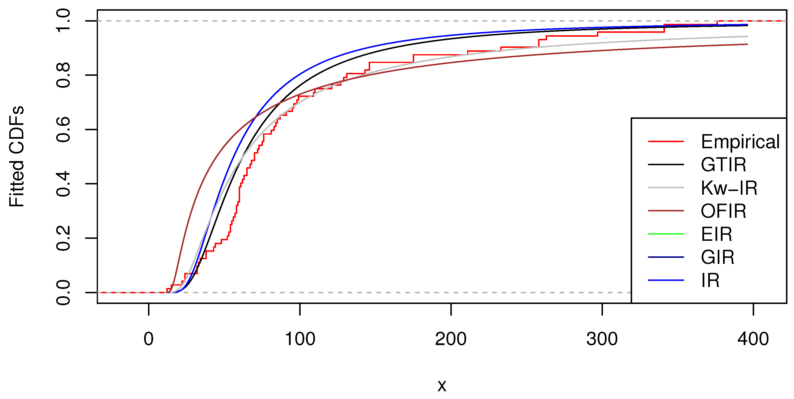
therefore, we reject the null hypothesis. Figure 4 illustrates the empirical cumulative distribution function (ECDF), GIR, OFIR, Kw-IR, EIR, and IR distributions for the data presented in Table 3.

The LSEs and MPSEs of ($\lambda ,\alpha$, $\sigma$) from the GTIR for data set I are given by:

• $({\widehat{\lambda }}_{\mathrm{MPS}},{\widehat{\alpha }}_{\mathrm{MPS}}$, ${\widehat{\sigma }}_{\mathrm{MPS}})=(-0.783,9.090,32.666),$
• (${\widehat{\lambda }}_{LS},{\widehat{\alpha }}_{LS}$, ${\widehat{\sigma }}_{LS})=(-0.677,8.047,33.033)$, and
• (${\widehat{\lambda }}_{CVM},{\widehat{\alpha }}_{CVM}$, ${\widehat{\sigma }}_{CVM})=(-0.725,7.814,31.125)$, respectively.

Dataset 2: The second dataset, collected by Nichols and Padgett [38], presents 100 observations on the breaking stress of carbon fibers of 50 mm in length. These data are showcased in

Table 5. Breaking stress data for carbon fibers (50 mm in length).

3.70	2.74	2.73	2.50	3.60	3.11	3.27	2.87	1.47	3.11
4.42	2.41	3.19	3.22	1.69	3.28	3.09	1.87	3.15	4.90
3.75	2.43	2.95	2.97	3.39	2.96	2.53	2.67	2.93	3.22
3.39	2.81	4.20	3.33	2.55	3.31	3.31	2.85	2.56	3.56
3.15	2.35	2.55	2.59	2.38	2.81	2.77	2.17	2.83	1.92
1.41	3.68	2.97	1.36	0.98	2.76	4.91	3.68	1.84	1.59
3.19	1.57	0.81	5.56	1.73	1.59	2.00	1.22	1.12	1.71
2.17	1.17	5.08	2.48	1.18	3.51	2.17	1.69	1.25	4.38
1.84	0.39	3.68	2.48	0.85	1.61	2.79	4.70	2.03	1.80
1.57	1.08	2.03	1.61	2.12	1.89	2.88	2.82	2.05	3.65

.

The results presented in

Table 6. Estimates and goodness-of-fit measures for different distributions for data set II.

Model	Parameters and (SEs)	$-2\mathit{\ell }$	AIC	AICC	BIC	KS
IR	$\sigma =3.275$ (0.327)	350.48	352.48	352.52	355.08	0.172
EIR	$\begin{array}{c}\alpha =3325.72\left(10.314\right)\\ \sigma =0.031\left(0.008\right)\end{array}$	350.54	354.54	354.66	359.75	0.173
OFIR	$\begin{array}{c}\sigma =0.495\left(0.037\right)\\ \alpha =0.837\left(0.080\right)\end{array}$	450.81	454.81	454.93	460.02	0.387
Kw-IR	$\begin{array}{c}a=1.322\left(0.211\right)\\ b=1.139\left(0.156\right)\\ \sigma =1.646\left(0.234\right)\end{array}$	349.68	355.68	355.93	363.49	0.189
GIR	$\begin{array}{c}\eta =1.139\left(0.165\right)\\ \rho =0.528\left(0.036\right)\end{array}$	349.68	355.68	355.81	358.89	0.189
GTIR	$\begin{array}{c}\lambda =-0.885\left(0.103\right)\\ \alpha =1.064\left(0.183\right)\\ \sigma =1.371\left(0.224\right)\end{array}$	335.13	341.13	341.38	348.94	0.154

indicate that, in terms of fitting the data, the generalized transmuted inverse Rayleigh distribution stands out as the most effective model among those considered. It demonstrates superior performance compared to the GIR, OFIR, Kw-IR, EIR, and IR distributions.

The likelihood ratio (LR) test statistic to test the hypotheses

$$H_0:\lambda =0,\alpha =1$$

vs.

$$H_1:\lambda \ne 0,\alpha \ne 1$$

for dataset II is

$$\omega =15.35>5.99={\chi }_{2;0.05}^2;$$

therefore, we reject the null hypothesis.

The LSEs and MPSEs of ($\lambda ,\alpha$, $\sigma$) from the GTIR for data set II are given by:

• $({\widehat{\lambda }}_{\mathrm{MPS}},{\widehat{\alpha }}_{\mathrm{MPS}}$, ${\widehat{\sigma }}_{\mathrm{MPS}})=(-0.870,1.045,1.369),$
• (${\widehat{\lambda }}_{LS},{\widehat{\alpha }}_{LS}$, ${\widehat{\sigma }}_{LS})=(-0.875,1.194,1.581)$, and
• (${\widehat{\lambda }}_{CVM},{\widehat{\alpha }}_{CVM}$, ${\widehat{\sigma }}_{CVM})=(-0.864,1.215,1.498)$, respectively.

16. Conclusions

In this article, we introduced the generalized transmuted inverse Rayleigh distribution, which offers a versatile and comprehensive framework for the statistical analysis of positive data. Parameter estimation is carried out using maximum likelihood, least squares, and maximum product spacing methods, alongside deriving asymptotic confidence intervals for the model parameters. We detail the quantile function, moments, harmonic mean, mean deviation, stress–strength reliability, and entropy. Additionally, we utilize the likelihood ratio test statistic to compare the model with its baseline counterpart. Two applications of the GTIR demonstrate its superior fit compared to other statistical models. We believe that our proposed model will find widespread applicability in addressing real-world problems across various disciplines, including medicine, engineering, and the social sciences.

17. Future Work

Future research can focus on further exploration and refinement of the Bayes estimators and maximum likelihood estimators for the unknown parameters of the generalized transmuted inverse Rayleigh distribution, especially in the context of both type I and type II censored samples.