Article

Direct and Inverse Kinematics of a 3RRR Symmetric Planar Robot: An Alternative of Active Joints

by
Jordy Josue Martinez Cardona
1,
Manuel Cardona
2,
Jorge I. Canales-Verdial
3 and
Jose Luis Ordoñez-Avila
1,*
1
Faculty of Engineering, Universidad Tecnológica Centroamericana (UNITEC), San Pedro Sula 21112, Honduras
2
Research Department, Universidad Don Bosco, Soyapango 1774, El Salvador
3
Mechatronics Department, Central New Mexico Community College, Albuquerque, NM 87106, USA
*
Author to whom correspondence should be addressed.
Symmetry 2024, 16(5), 590; https://doi.org/10.3390/sym16050590
Submission received: 20 March 2024 / Revised: 19 April 2024 / Accepted: 20 April 2024 / Published: 10 May 2024
(This article belongs to the Special Issue Symmetry in Mechanical Engineering: Properties and Applications)

Abstract

:
Existing direct and inverse kinematic models of planar parallel robots assume that the robot’s active joints are all at the bases. However, this approach becomes excessively complex when modeling a planar parallel robot in which the active joints are within one single kinematic chain. To address this problem, our article unveils an alternative for a 3RRR symmetric planar robot modeling technique for the derivation of the robot workspace and the analysis of its direct and inverse kinematics. The workspace was defined using a system of inequalities, and the direct and inverse kinematics models were generated using vectorial analysis and an optimized geometrical approach, respectively. The resulting models are systematically presented and validated. Two final model renditions are delivered supplying a thorough equation analysis and an applicability discussion based on the importance of the robot’s mobile platform orientation. The advantages of this model are discussed in comparison to the traditional modeling approach: whereas conventional techniques require the solution of complex eighth-degree polynomials for the analysis of the active joint configuration of these robots, these models provide an efficient back-of-the-envelope analysis approach that requires the solution of a simple second-degree polynomial.

Graphical Abstract

1. Introduction

Kinematic models supply a practical mathematical analysis toolbox to predict robotic operation performance. Robot kinematics can be defined as an analytical method that describes a robot’s spatiotemporal motion by modeling the relationship between a robot’s joint positions and its end-effector’s position and orientation coordinates [1]. Direct kinematic models begin with the joint position variables and yield the resulting end-effector’s position and orientation coordinates. Moreover, direct kinematics harness geometric methods to derive models by the implementation of homogeneous transformation matrices, the Denavit–Hartenberg algorithm, and the use of quaternions [2]. In contrast, inverse kinematics reverse the approach starting first with a desired end-effector position and orientation and then ascertains the required robot joint position values. Nonetheless, despite being a counterpart to direct kinetics, inverse kinematic models can also be derived via geometric methods; in this case, however, it is through means of homogeneous transformation matrices, kinematic decoupling, and Screws theory [2,3].
Robot kinematic models exist to comprehend a robot’s motion and conduct an operation performance analysis. These models must facilitate the engineer’s decision making and design the action-planning process. However, traditional modeling approaches for 3RRR parallel planar robots [3,4,5,6,7,8,9,10,11,12] do not provide simple models for robot configurations with active joints that are all placed within one single kinematic chain. The traditional models with the active joints located at the bases actually render the modeling of single kinematic chain active joint robots as a complex task that requires solving computing-intensive calculations. Therefore, the originality of this paper is the kinematic modeling of 3RRR parallel planar robots with single kinematic chain active joints. These kinematics are demystified by providing a simplified approach that reduces the computational task from a burdensome eighth-degree polynomial model to a simple back-of-the-envelope solvable mathematical model.

1.1. Planar Parallel Robots

An industrial robot is an automatically controlled, reprogrammable, and multipurpose manipulator with at least three independent movements (degrees of freedom); for use in manufacturing processes, this manipulator has the ability to move a variety of functional objects through previously configured movements for the purpose of performing different tasks [13]. Robots can be classified into open and closed kinematic chain robots. Open-chain robots, which have links that are connected in series, have become ubiquitous in industrial robotic applications. In the case of the 3RRR, which has three independent closed kinematic chains, the characteristics of symmetry allow for the mathematical modeling of one of the chains and generalization to the other two. The subset of planar robots in which the motion is restricted to a single 2D plane is called planar parallel robots. Considering the R label for revolute joints and P label for prismatic joints, the possible configurations for parallel planar robots are depicted in Figure 1. The PPP configuration is not feasible due to the lack of independence. The end effectors are situated at the centroid of the internal triangle of the robot, enabling it to perform tasks in soft robotics [14,15], traditional pick-and-place operations [16], and even medical applications [17].
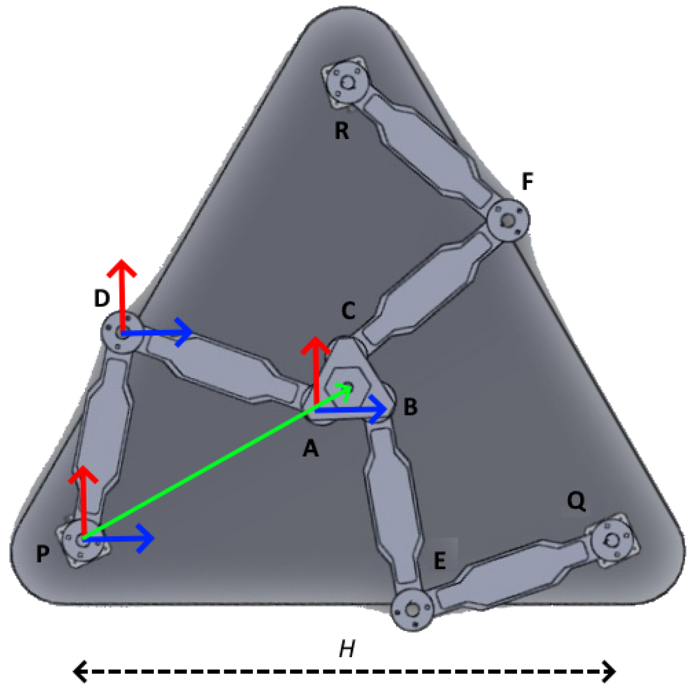
The particular 3RRR symmetric planar robot studied in this work is shown in Figure 2. This robot contains six chain links that may be of different or equal sizes and a triangular chain that joins the three interdependent kinematic chains and acts as the tool center point. Moreover, this planar robot’s movement is restricted to 2D-planar motion. Generally, parallel robots that do not exhibit singularities are isotonic. Therefore, using Grubler’s formula, it is determined that this robot contains only three degrees of freedom: x, y, and ϕ , where x and y describe the robot’s position with respect to the Cartesian plane and ϕ corresponds to the orientation angle that the end-effector forms with the horizontal. Given this robot configuration, kinematic models are required to describe the robot’s operation motion.
The planar robots studied in this research apply the similarity law (six chains of the same size); this means the robot has geometic symmetry [18,19,20,21]. Also, symmetry is present in the Jacobian matrix condition index, which can be evidenced by graphically observing the distribution of the condition index throughout the workspace [3]. Additionally, the symmetry of parallel robots is present in the differential mathematical model, which is represented through Jacobian matrices [18].

1.2. Existing 3RRR Symmetric Planar Robot Kinematic Models

Mathematical models exist in the literature for the analysis of articulated parallel robots. Table 1 shows an approach comparison among the modeling methods used by researchers, including the active joints for the mathematical modeling techniques, which were implemented to derive direct and inverse kinematics. Geometric models have the advantage of being more conventional, allowing the planar robot to move with speed and precision. The main disadvantage of geometric models is the computational expense due to the complexity of their kinematic equations. The advantage of screw theory is that it enables the development of a simple dynamic model with which controllers can be developed.
Among the referenced literature, it is observed that most articles base their analyses under the assumption that the active joints are all placed at the kinematic chain bases in P, Q, and R in Figure 2. The only exception is [22], which studies two additional configurations but limits its analysis to the singularities. It is also observed that the geometric method is the most common approach to derive both direct and inverse kinematic models. However, this approach yields eighth-degree polynomial-based models, which must be solved via the implementation of large-scale computational resources. Moreover, solving these conventional mathematical models generates eight possible solutions to configure the position angles of the robot’s active joints, which also increments workspace robot singularities.
Non-articulated planar parallel robot modeling has also been actively studied in P, D, and A joints [23,24,25,26,27,28] and cable-driven planar robots [29,30,31,32]. Furthermore, the applications of these planar parallel robots can range from window-washing applications [29] to orthopedics [23,25] and even neurorehabilitation [33]. Hence, the models derived in this paper may be applied to all the referenced literature in this section and broaden the body of knowledge of the planar parallel robot.

1.3. 3RRR Symmetric Planar Robot Active Joints

Robotic joints are the mechanical connections between chain links. A robotic joint can be categorized according to its kinematic design into revolute (R), prismatic (P), screw (H), cylindrical (C) universal (U), spherical (S), or parallelogram (Pa) joints. Each of these joints can be further classified into active or passive joints. Active joints, notated by an underscored joint abbreviation, exert a controlled force to generate a robotic position shift. Active joints utilize motors to control robotic motion and orientation. In contrast, passive joints move through externally actuated forces transmitted by kinematic chains.
This study focuses on the 3RRR symmetric planar robot shown in Figure 2. Existing literature models [3,4,5,6,7,8,9,10,11,12] position active joints at the base joints, i.e., P, Q, and R, whereas passive joints are at points A, B, C, D, E, and F. This study proposes a mathematical model of a planar parallel robot where the active joints are rather located at joints P, D, and A, all of which belong to a single kinematic chain. The kinematic models derived in this work are then compared and contrasted to the conventional models in Table 1, and a discussion of the advantages of our derived models is provided.

2. Methods

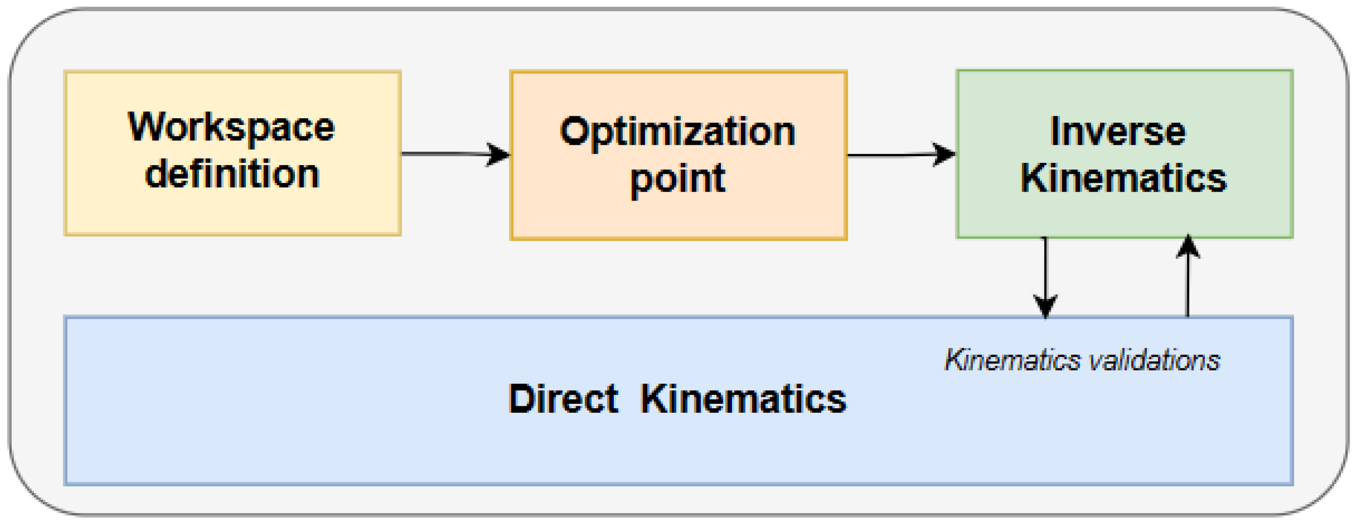
This work aims to develop the forward kinematics and inverse kinematics of a 3RRR planar robot with its active joints in a kinematic chain. To achieve this, several concepts are developed, starting with the definition of the workspace and followed by orientation points, inverse kinematics, and finally forward kinematics, which validate all previous models as shown in Figure 3.
Also, some assumptions and methods are taken for the kinematic model derivation, including the following:
  • The location of the robot’s active joints was taken at joints P, D, and A, as shown in Figure 2.
  • Joints Q, E, B, C, F, and R in Figure 2 are all passive joints.
  • The mathematical methods implemented for model derivation are the law of cosines, trigonometric properties, geometric relations, the Pythagoras theorem, derivatives, vectors, and matrices.
  • The mathematical models obtained are the workspace, the direct kinematics models, and the inverse kinematics models.
  • The workspace is defined using a system of inequalities provided by the constraints from the lengths of the fully extended kinematic chains.
  • The derivation of the direct kinematics model is approached via vectorial analysis.
  • The inverse kinematic model is derived through the geometric method and optimization techniques.
  • Model validation is achieved using MATLAB-based software corroboration.
The following parameter definitions were also conducted for model derivation:
Take H as the distance between the base joints in the planar robot, i.e., the length of segments P Q ¯ , Q R ¯ , and P R ¯ . Moreover, to reduce the robot singularities, all chains are assumed to be of equal length l and the end-effector is assumed to have the fixed dimensions of an equilateral triangle platform [3]. Hence, the dimensions of the chains and the end-effector sides can be calculated by (1) and (2):
h = 1 10 H
l = 2 5 H
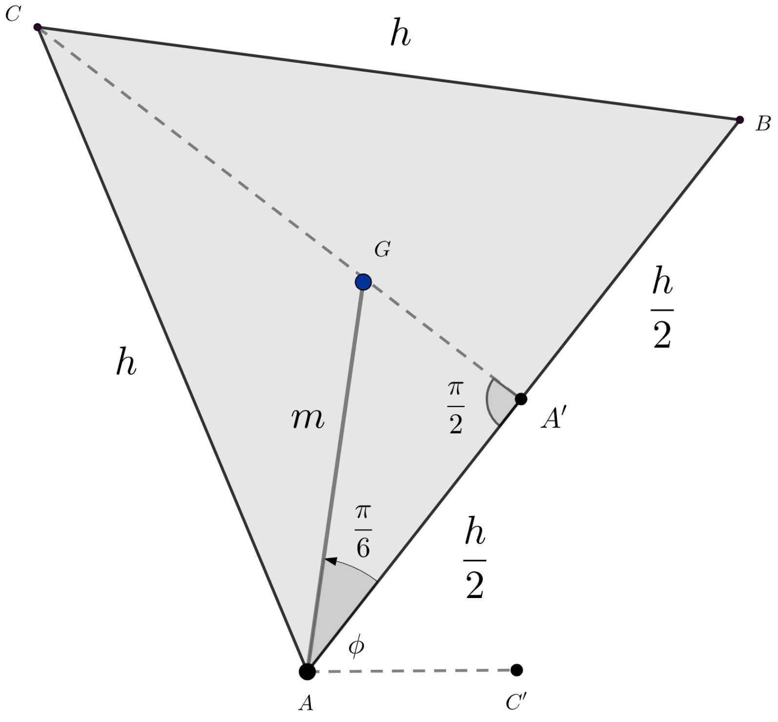
where l is the length of each of the robot’s six chains and h is the length of the three sides of the mobile platform’s end-effector [3]. Furthermore, the distance from vertex point A to the centroid point G of the end-effector (as shown in Figure 4) must also be considered.
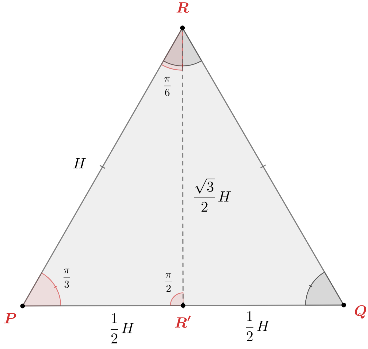
Given that point G is the centroid of the equilateral-triangle-shaped end-effector, Δ A B C , let segment A G ¯ be equal to m, as shown in Figure 4. Furthermore, when the segment C G ¯ is extended, it bisects segment A B ¯ at point A . Moreover, given that the orthocenter, incenter, and centroid of an equilateral triangle are all the same point, then A A ¯ = A B ¯ = h 2 , C A A = π 2 , and G A A = π 6 . Furthermore, since Δ A G A is a right triangle, the definition of the cosine trigonometric function (3) is used to find m in (4):
cos π 6 = A A ¯ A G ¯
Given that cos π 6 = 3 2 , A A ¯ = h 2 , and A G ¯ = m , isolating m leads to
m = h 3
Then, using Equation (1) and rationalizing, m becomes a function of H:
m = 1 10 H 1 3
m = 1 10 3 H
m = 3 30 H
This method is applicable to symmetric 3RRR planar robots, which use parameters H, h, and l as design parameters, where l and h depend on H at the moment of designing the robot. Additionally, the active joints are located in one of the robot’s kinematic chains. To perform the calculations, MATLAB was used, in which functions were developed for both the direct kinematics and the inverse kinematics of the robot.

3. Results

3.1. Workspace Definition

Taking each of the robot’s kinematic chains with a specific position in a Cartesian reference plane [34], let point G with coordinates ( P x , P y ) be the final position of the end-effector’s centroid. Then, to derive the robot’s workspace, consider the delimitations given by the kinematic chain constraints.

3.1.1. First Kinematic Chain Workspace Constraints

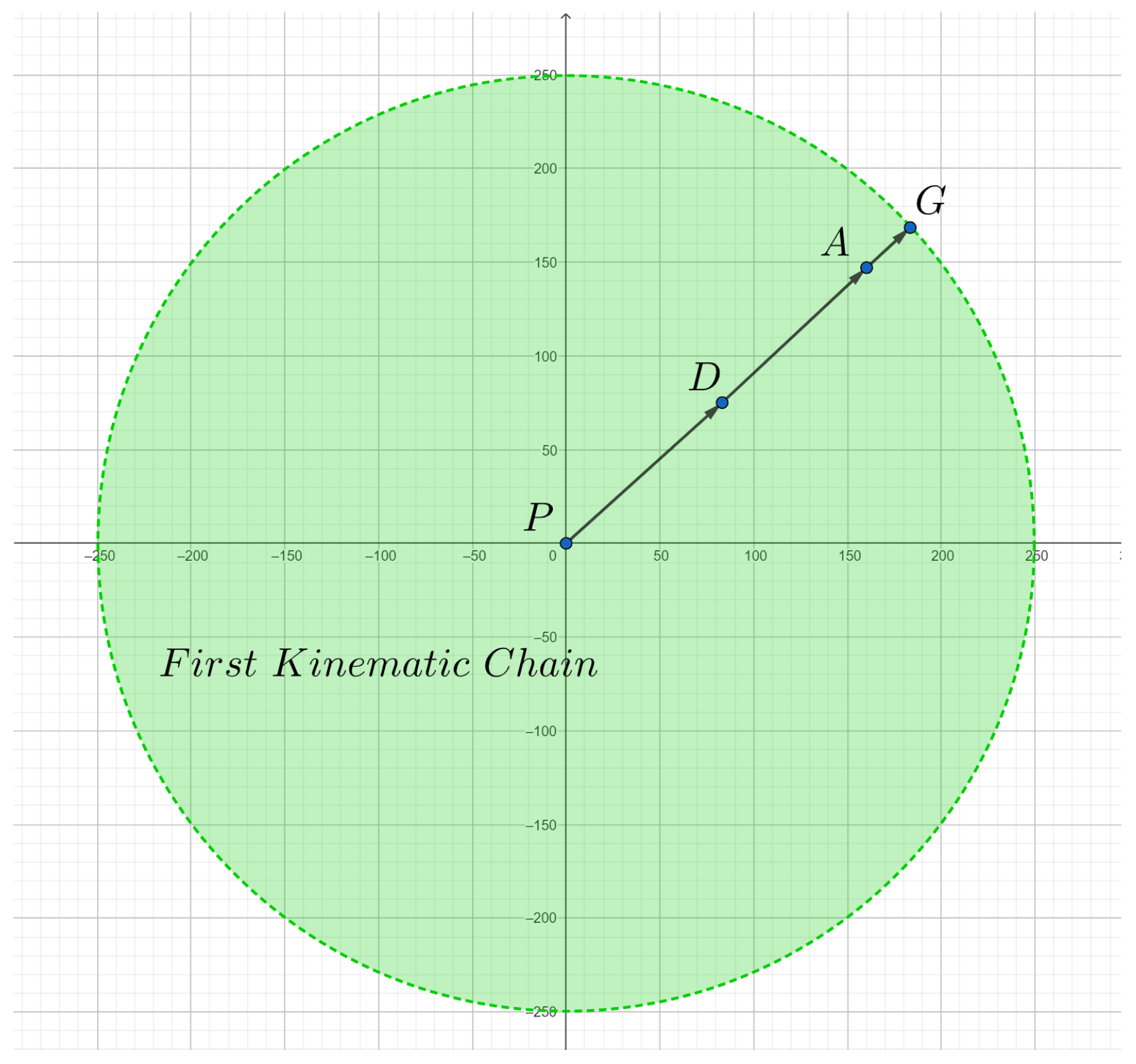
The first kinematic chain, composed of links P D ¯ , D A ¯ , and A G ¯ , has active joints at all three of its articulations P, D, and A. Moreover, its base articulation P is set at position ( 0 , 0 ) . Then, letting G, with coordinates ( P x , P y ) , be all the possible positions that the end-effector’s centroid can reach, the inequality shown in expression (8) is derived. This expression acts as the first workspace constraint, where the end-effector’s position is limited by the length of the fully extended first kinematic chain, and it is shown in Figure 5:
P x 2 + P y 2 < ( 2 l + m ) 2
Note that the workspace has been defined using less-than inequalities to avoid working mode misconfigurations. Whereas the conventional planar parallel robot kinematic models provide eight solutions to this robot configuration, only two of them have no singularities in their workspace [3]. In this research, by making the workspace definitions less-than inequatities, we prevent the robot from reaching potential working modes that, due to inertia, could result in a misconfiguration of the position of the kinematic chains. Hence, the models presented in this work yield two viable non-singular positions within the workspace: (1) a position when all kinematic chains are oriented elbow-down and (2) when they are oriented elbow-up.

3.1.2. Second Kinematic Chain Workspace Constraints

The second kinematic chain, composed of links R F ¯ , F C ¯ , and C G ¯ , has a passive joint in all three of its articulations R, F, and C. Moreover, this chain’s base joint, R, has a fixed position given by coordinates 1 2 H , 3 2 H , as shown in Figure 6.
Hence, the inequality shown in expression (9) further delimits the robot’s workspace due to the second kinematic chain’s length. As with the first kinematic chain, the distance from C G ¯ must be taken into consideration. However, given that Δ A B C is an equilateral triangle, A G ¯ = B G ¯ = C G ¯ = m ; hence, (9) provides the second workspace constraint:
P x H 2 2 + P y 3 2 H 2 < ( 2 l + m ) 2
This expression further reduces the robot’s workspace as shown in Figure 7 because the allowed final end-effector position, G, must satisfy both (8) and (9).

3.1.3. Third Kinematic Chain Workspace Constraints

The third kinematic chain, composed of links Q E ¯ , E B ¯ , and B G ¯ , has passive joints in all three of its articulations Q, E, and B. Moreover, its base joint Q has a fixed position given by coordinates ( H , 0 ) , as shown in Figure 6. Hence, analogously to the workspace constraint expressions derived for the first two kinematic chains, the end-effector’s final position G is delimited by expression (10):
( P x H ) 2 + P y 2 < ( 2 l + m ) 2
Therefore, the end-effector’s final position G, with coordinates ( P x , P y ) , must satisfy all three inequality expressions (8)–(10), as shown in Figure 8.
Thus, this workspace description method offers a novel and straightforward approach. This system of inequalities can be visualized as the common area of three symmetric circles. These inequality systems will be utilized for both the direct and inverse kinematics of the study in the next two sections.

3.2. Direct Kinematics Model

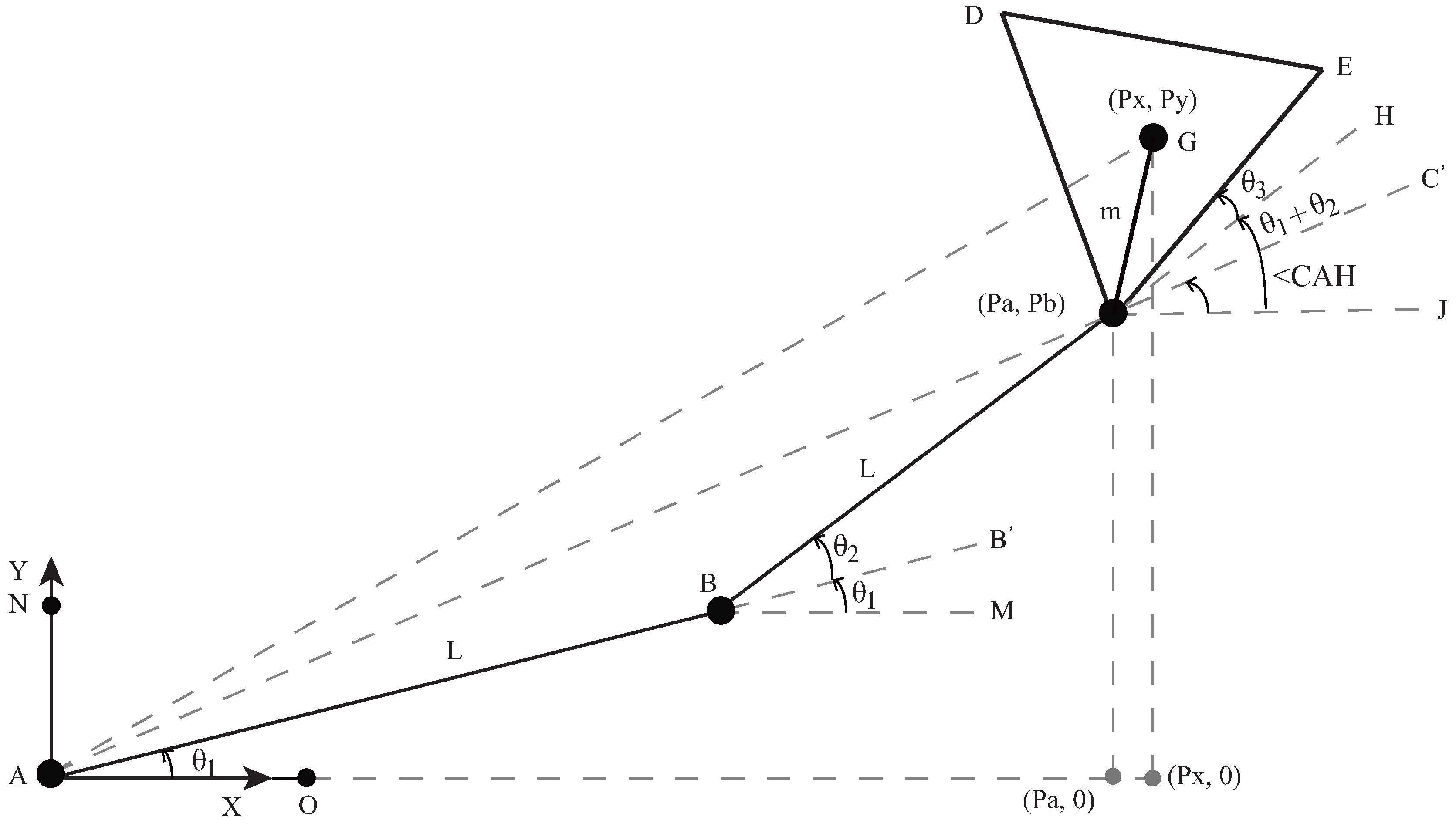
The reference system is located at the active joint A according to Figure 9. Hence, P x and P y will be referenced there. To obtain the direct kinematics, a vector addition is used, where the links A B ¯ , B C ¯ , and C G ¯ will determine the vectors. The result of the vector A G is given in (11):
A B + B C + C G = A G
In Figure 9, each vector can be broken down into its components, as shown in (12)–(14):
A B = ( l cos θ 1 ) i ^ + ( l sin θ 1 ) j ^
B C = [ l cos ( θ 1 + θ 2 ) ] i ^ + ( l sin ( θ 1 + θ 2 ) ) j ^
C G = m c o s θ 1 + θ 2 + θ 3 + π 6 i ^ + m sin θ 1 + θ 2 + θ 3 + π 6 j ^
If A G = P x i ^ + P y j ^ is the vector sum of (11), then the following Equations (15) and (16) are obtained for each component of the vector A G :
P x = l cos θ 1 + l cos ( θ 1 + θ 2 ) + m c o s θ 1 + θ 2 + θ 3 + π 6
P y = l sin θ 1 + l sin ( θ 1 + θ 2 ) + m sin θ 1 + θ 2 + θ 3 + π 6
To obtain the orientation of the triangular chain Δ C D E , the angle E C J is analyzed. From here, it is deduced that
ϕ = θ 1 + θ 2 + θ 3
In conclusion, Equations (15)–(17) describe the 3-DOF that the 3RRR symmetric planar robot can have.

3.3. Inverse Kinematics Model

The geometric method will be utilized to determine the inverse kinematics. To achieve this, we analyze Figure 9, depicting the motorized kinematic chain of the robot.
Point C with coordinates ( P a , P b ) is defined, which will help find the angles of the active joints θ 1 , θ 2 , and θ 3 in terms of these coordinates and the final position G with coordinates ( P x , P y ) .
The first step is to analyze the chains AB and BC.
Solution for θ 1 : Based on [35], if we analyze the angles forming N A O , it can be expressed as (18):
N A O = N A C + C A B + θ 1
Since N A O = π 2 is an angle of the reference coordinate system, if θ 1 is isolated, then (19) occurs:
θ 1 = π 2 N A C C A B
To find angle N A C , it is observed that the segments N A and C H are parallel since the sum of angles N A O and A H C equals π . Therefore, N A C = A C H . So, A C H is obtained by (20):
cos ( A C H ) = C H C A
If C H = P b , C A = P a 2 + P b 2 , and N A C = A C H , if A C H is isolated and substitutes the other variables, the result is (21):
N A C = arccos P b P a 2 + P b 2
To obtain C A B , the triangle Δ C A B is analyzed; using the cosine law on this triangle, the following is obtained (22):
C D 2 = C A 2 + A B 2 2 ( C A ) ( A B ) cos ( C A B )
If C B = A B = l and C A = P a 2 + P b 2 , then (23):
l 2 = P a 2 + P b 2 + l 2 2 l P a 2 + P b 2 cos ( C A B )
If C A B is isolated, (24):
C A B = arccos P a 2 + P b 2 2 l P a 2 + P b 2
Therefore, replacing Equations (21) and (24) in (19), θ 1 is obtained in terms of known variables using (25):
θ 1 = π 2 arccos P b P a 2 + P b 2 arccos P a 2 + P b 2 2 l P a 2 + P b 2
Solution for θ 2 : The triangle Δ A B C is analyzed [35], from which it is deduced that in (26),
A C ¯ 2 = A B ¯ 2 + B C ¯ 2 2 ( A B ¯ ) ( B C ¯ ) cos ( A B C )
If C A ¯ = P a 2 + P b 2 and C B ¯ = A B ¯ = l , then (27):
P a 2 + P b 2 = l 2 + l 2 2 ( l ) ( l ) cos ( A B C )
Isolating for cos ( A B C ) results in (28):
cos ( A B C ) = P a 2 + P b 2 2 l 2 2 l 2
If A B C = 180 θ 2 , then (29):
cos ( 180 θ 2 ) = P a 2 + P b 2 2 l 2 2 l 2
By the trigonometric property cos ( 180 θ ) = cos ( θ ) , cos ( 180 θ 2 ) = cos θ 2 ; therefore, (30).
cos ( θ 2 ) = P a 2 + P b 2 2 l 2 2 l 2
Isolating for θ 2 , it is deduced that (31):
θ 2 = arccos P a 2 + P b 2 2 l 2 2 l 2
Solution for θ 3 : The triangle Δ A C G is analyzed, and it is deduced that (32):
A G ¯ 2 = A C ¯ 2 + C G ¯ 2 2 ( A C ¯ ) ( C G ¯ ) cos ( A C G )
If A G ¯ = P x 2 + P y 2 , C A ¯ = P a 2 + P b 2 and C G ¯ = m , then (33):
P x 2 + P y 2 = P a 2 + P b 2 + m 2 2 m P a 2 + P b 2 cos ( A C G )
Isolating for cos ( A C G ) results in (34):
cos ( A C G ) = P x 2 + P y 2 P a 2 P b 2 m 2 2 m P a 2 + P b 2
If A C G = 180 G C C , then (35):
cos ( 180 G C C ) = P x 2 + P y 2 P a 2 P b 2 m 2 2 m P a 2 + P b 2
Since cos ( 180 G C C ) = cos G C C , then (36):
cos ( G C C ) = P x 2 + P y 2 P a 2 P b 2 m 2 2 m P a 2 + P b 2
By trigonometry properties, it is known that tan 2 ( G C C ) + 1 = sec 2 ( G C C ) . Isolating for G C C , it is deduced that G C C = arctan ( ± sec 2 ( G C C ) 1 ) . If sec ( G C C ) = 1 cos ( G C C ) , using Equation (36), (37) is deduced:
G C C = arctan ± 2 m P a 2 + P b 2 P x 2 + P y 2 P a 2 P b 2 m 2 2 1
This result generated two solutions for G C C . It would be necessary to validate which of the two solutions is the correct one. For this, the answers will be validated using the direct kinematics of the robot proposed in this research.
If the angles between the angle G C J are analyzed, (38):
θ 1 + θ 2 + θ 3 + π 6 = G C C + C C J
If C C J = C A H , and if θ 3 is isolated, then (39):
θ 3 = G C C + C A H θ 1 θ 2 π 6
If C A H = arctan P b P a , substituting in Equation (39), it is concluded that (40):
θ 3 = arctan P b P a + arctan ± 2 m P a 2 + P b 2 P x 2 + P y 2 P a 2 P b 2 m 2 2 1 θ 1 θ 2 π 6
Therefore, Equations (25), (31) and (40) describe the inverse kinematics of the robot. To reach position ( P x , P y ) , the inverse kinematics will give two possible results, which must be validated using the direct kinematics to identify the correct angle configuration θ 1 , θ 2 , and θ 3 .

Solution for P a and P b

Figure 10 represents the geometry of a mobile platform; all the parameters P a and P b are utilized. These parameters depend on the initial parameters P x and P y , selected from a mathematical equation. Additionally, P a and P b could be contingent upon the orientation angle ϕ , though it is essential to ascertain if the orientation of the robot truly impacts its application. An analysis will be conducted to determine the values of P a and P b in two scenarios: one where the orientation ϕ of the triangle Δ C D E is significant and another where it is not. In the latter case, the solutions will be based on a criterion involving the minimum distance from the active joints 1 and 3.
Solution for P a and P b where the orientation ϕ matters.
It is assumed that P x and P y belong to the workspace. From Figure 10, if G C C = π 6 + ϕ , then the following Equations (41) and (42) can be deduced:
P x P a = m cos π 6 + ϕ
P y P b = m cos π 6 + ϕ
Isolating for P a in (41) and P b in Equation (42), the required values would be found to have the complete inverse kinematics considering the orientation ϕ (43) and (44):
P a = P x m cos π 6 + ϕ
P b = P y m sin π 6 + ϕ
Solution for P a and P b where the orientation ϕ does not matter:
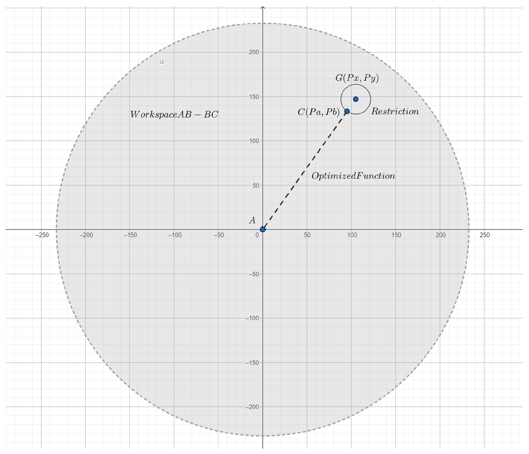
Given that ( P x , P y ) is the desired position of the robot, in this case, ϕ is not considered in this analysis and the point ( P a , P b ) is taken using the following criterion: ( P a , P b ) is the minimum possible distance from active joint 1; in other words, from point A according to Figure 9. From this criterion, the problem needs a solution using optimization. Also, by geometry, ( P a , P b ) has a workspace given by the two chains A B ¯ and B C ¯ that can be defined by the following inequality (45):
P a 2 + P b 2 < 4 l 2
For this problem, a function to optimize and a restriction are needed. The optimization function is the distance between the active joints 1 and 3, which will be denoted by r. Putting it into an equation results in (46) as shown in Figure 11:
r 2 = P a 2 + P b 2
The only restriction that this case has is the distance between point G, where the end-effector is located, and point C, where the active joint is located, so (46):
m 2 = ( P x P a ) 2 + ( P y P b ) 2
From here, P b is isolated, taking the positive square root of the process, and replaced in (46). So, the function to optimize is (48):
r 2 = P y m 2 ( P x P a ) 2 2 + P a 2
The derivative of r with respect to P a is taken, and (49) is deduced:
d r d P a = P y P a + P x m 2 ( P x P a ) 2 P y P x m 2 ( P x P a ) 2 P a 2 + P y m 2 ( P x P a ) 2 2
Let d r d P a = 0 , and the value of P a that satisfies the equation is found by (50):
P y P a + P x m 2 ( P x P a ) 2 P y P x = 0
By doing arithmetic operations, it follows that (51) occurs:
( P x 2 + P y 2 ) P a 2 + ( 2 P x P y 2 2 P x 3 ) P a + ( P x 2 P y 2 P x 2 m 2 + P x 4 ) = 0
In order to work in a more organized manner, it is stated that a = P x 2 + P y 2 , b = 2 P x P y 2 2 P x 3 , and c = P x 2 P y 2 P x 2 m 2 + P x 4 , so (52):
a P a 2 + b P a + c = 0
By the quadratic equation, the roots of the equation are found by (53):
P a = b ± b 2 4 a c 2 a
Since there are two results of P a , there must be two points: ( P a 1 , P b 1 ) and ( P a 2 , P b 2 ) . The point P b is determined with (54):
P b = P y m 2 ( P x P a ) 2
When isolating for P b , the positive square root was taken. Now, the negative square will be taken and the same process will be performed, so P b is now as shown in (55):
P b = P y + m 2 ( P x P a ) 2
Consequently, the new function to optimize is the following (56):
r 2 = P y + m 2 ( P x P a ) 2 2 + P a 2
If the derivative of d r d P a of Equation (56) is calculated, the derivative equals zero, and P b is isolated, the solution for P a is exactly the same as Equation (51). Since there are two solutions for P a in that case, there are two more solutions: ( P a 3 , P b 3 ) and ( P a 4 , P b 4 ) .
In brief, this proposed criterion will give four different answers obtained, as shown in Table 2.
To find out which of the four possible points to use, (46) is used to determine which generates the smallest distance r. Realizing a rigorous analysis of finding the expression that generates the smallest result, it is found that solution 2 generates the smallest distance r. Then, to generate the smallest distance between joint 1 and joint 3, (57), and (58) must be used:
P a = b b 2 4 a c 2 a
P b = P y m 2 ( P x P a ) 2
The summary of the most relevant equations for the development of functions in Matlab is shown in Figure 12. In the inverse kinematics, an equation from the forward kinematics is used to determine the correct value of θ 3 . And, a = P x 2 + P y 2 , b = 2 P x P y 2 2 P x 3 , and c = P x 2 P y 2 P x 2 m 2 + P x 4 .

4. Model Validation

4.1. Kinematics Model Implementations

Prior to employing direct and inverse kinematics, it is imperative that the desired point ( P x , P y ) of the 3RRR symmetric planar robot belongs to the workspace defined by the inequalities (8), (9) and (10).
The inverse kinematics model, in the two approaches explained (considering the orientation ϕ of the mobile platform Δ C D E ), will invariably produce two possible solutions for the angle configurations necessary to reach the desired point ( P x , P y ) . The correct angle selection is determined by inputting these angle values into the direct kinematics to verify if the data obtained correspond to the primary values inputted in the inverse kinematics. An algorithm is employed to ascertain the correct angles.
For example, let H = 136 , P x = 136 , P y = 16 , and ϕ = π 4 . In this scenario, the values of P x and P y satisfy the three inequalities of the workspace. Therefore, it is feasible for the robot to reach that location. Subsequently, if Equations (1), (2) and (4) are obtained using the aforementioned parameters, then l = 92 , m = 13.28 , and h = 23 , respectively. With this data, the equations describing the inverse kinematics are employed. If Equations (25), (31) and (40) are utilized,
  • If the orientation of the mobile platform Δ C D E is considered, then, employing Equations (43) and (44) to determine P a and P b , the two solutions in the form ( θ 1 , θ 2 , θ 3 ) for this case would be ( 42 . 52 ° , 87 . 78 ° , 0 . 26 ° ) and ( 42 . 52 ° , 87 . 78 ° , 147 . 52 ° ) , respectively.
There are two solutions, and to determine the correct one, the solutions are inputted into the direct kinematics to obtain the resulting values. For the first solution ( θ 1 , θ 2 , θ 3 ) = ( 42 . 52 ° , 87 . 78 ° , 0 . 26 ° ) , the direct kinematics yield P x = 136 , P y = 16 , and ϕ = 45 ° . For the second solution ( 42 . 52 ° , 87 . 78 ° , 147 . 52 ° ) , the direct kinematics yield P x = 136.61 , P y = 9.47 , and ϕ = 102 . 26 ° . Therefore, the correct configuration of angles is the first one.
  • If the orientation of the mobile platform Δ C D E is not considered, then utilizing Equations (57) and (58) to determine P a and P b , respectively, yields the two identical solutions in the form ( θ 1 , θ 2 , θ 3 ) , which are both ( 41 . 52 ° , 95 . 55 ° , 77 . 77 ° ) .
If the solution is validated in the direct kinematics, then the result would be P x = 136 , P y = 16 , and ϕ = 23 . 29 ° . Therefore, P x and P y are exactly as desired, but ϕ is different. However, this discrepancy is inconsequential as the angle ϕ is deemed unconsidered for the application.
To verify the proposed equations in the inverse kinematics and direct kinematics models, functions were implemented in MATLAB. These functions were used to ensure that the data from the inverse kinematics corresponded to those from the direct kinematics and vice versa. The conducted tests are presented in Table 3 and Table 4, where the parameter H is varied across different values, thus causing the values of h, m, and l to adjust accordingly. This illustrates how the direct and inverse equations are utilized to showcase the values of certain desired points and their corresponding angles required to reach those positions. Table 3 presents the results using the model where the orientation ϕ was considered, and Table 4 demonstrates the outcomes using the model where ϕ was not considered and an optimization process was executed.

4.2. Analysis of the Optimization of ( P a , P b )

Now for the optimization, it is crucial to understand the relationship between the two mathematical models found, both considering and not considering the orientation ϕ and how they can be compared. Basic statistical calculations will be employed to describe Table 5, which will contain the desired values P x and P y of the end-effector along with the two possible solutions. The standard deviation will be computed from each column of the table containing the angles. Additionally, it is noted that H = 230 and ϕ = 45 ° are constants. A total of 100 data points were collected to calculate the standard deviation. The table below presents a subset of 20 points.
Then, if the standard deviation of each one of the columns that corresponds to an angle is included, the results are shown in Table 6.

5. Discussion

In general, parallel robots offer several advantages over robotic arms, such as high speed and the ability to move masses, although they often have limitations in terms of their workspace and the complexity of kinematic equations [36]. This paper proposes a solution that preserves the advantages of parallel robots while reducing the complexity of kinematic equations by a vector analysis. The presented algorithm offers two alternatives: the traditional one, which requires knowledge of the orientation phi of the end-effector and is used in various applications as pick and place [37,38], or medical rehabilitation [39,40]. There is also an alternative that eliminates the need to know this orientation, using instead an optimization method, useful in monitoring applications like conventional or thermal cameras [41]. This means that the similarity law of planar 3RRR robots reduces the number of singularities obtained in kinematic models. Most models use P, Q, and R as active joints [3,4,5,6,7,8,9,10,11,12], which is the major difference from this kinematic model, which has active joints in P, D, and A. This complexity in kinematic models leads to the use of polynomial equations of degree eight for their solution. The workspace of this model is delimited by the areas common to the circles generated in P, Q, and R with the sum of the links as the radius. The main contribution of this work is the proposal of a new alternative for the implementation of planar 3RRR robots. This proposal has (15)–(17) as direct kinematics and (25), (31) and (40) as inverse kinematics. For applications where phi is not necessary, the application of inverse kinematic systems is proposed.

6. Conclusions

The development of a mathematical model for robots of this type can be challenging, with the aim of simplifying their behavior description. This research has led to the creation of a mathematical model that achieves this goal, offering a simpler alternative to the traditional approach. Despite being based on conventional methods, the mathematics of this model is notably more user-friendly. Basic mathematical tools and optimization techniques were employed in its development, aiming to streamline robot motion. An initial optimization analysis yielded promising standard deviations, yet further evaluation using more sophisticated statistical methods is warranted to fully assess the method’s efficiency. Moreover, there is still much to explore, including the differential kinematics model and dynamic considerations, to draw comprehensive conclusions regarding the robot’s positioning and configuration. As a future endeavor, the aim is to develop the dynamic model of this planar robot and conduct comparisons to assess its advantages and disadvantages relative to traditional models.

Author Contributions

Conceptualization, J.L.O.-A.; Methodology, J.L.O.-A.; Validation, M.C.; Formal analysis, J.J.M.C.; Investigation, J.J.M.C. and J.I.C.-V.; Writing—original draft, J.J.M.C.; Writing—review & editing, J.I.C.-V. and J.L.O.-A.; Visualization, M.C. and J.I.C.-V. All authors have read and agreed to the published version of the manuscript.

Funding

This work was supported by the Research Fund of Universidad Tecnológica Centroamericana (UNITEC), Honduras.

Data Availability Statement

Data are contained within the article.

Acknowledgments

This work was supported by the Research Fund of Universidad Tecnológica Centroamericana (UNITEC), Honduras.

Conflicts of Interest

The authors declare no conflict of interest.

References

  1. Torres Vargas, L.Z. Introducción a la Robótica; Grupo Editorial Éxodo: Miguel Hidalgo, Mexico, 2012. [Google Scholar]
  2. Barrientos, A. Fundamentos de Robótica, 2nd ed.; McGraw-Hill España: Madrid, Spain, 2012. [Google Scholar]
  3. Cardona, M.N. Similarity law for the design and workspace optimization of 3RRR planar parallel robots. In Proceedings of the 2014 IEEE Central America and Panama Convention (CONCAPAN XXXIV), Panama City, Panama, 12–14 November 2014; pp. 1–6. [Google Scholar] [CrossRef]
  4. Serrano, F.; Rodriguez, B.; Cardona, M. Obtención de un Modelo Dinámico Para un Robot 3RRR Basado en Teoría de Screws. Rev. Iberoam. Autom. E Inform. Ind. 2018, 15, 384–390. [Google Scholar] [CrossRef]
  5. Rodelo, M.; Villa, J.; Duque, J.; Yime, E. Kinematic Analysis and Performance of a Planar 3RRR Parallel Robot with Kinematic Redundancy using Screw Theory. In Proceedings of the 2018 IEEE 2nd Colombian Conference on Robotics and Automation (CCRA), Barranquilla, Colombia, 1–3 November 2018; IEEE: Barranquilla, Colombia, 2018; pp. 1–6. [Google Scholar] [CrossRef]
  6. Martinez-Zamudio, P.; Gonzalez-Villela, V.J.; Lopez-Parra, M.; Ramirez-Reivich, A.C. Cinemática Diferencial de un Manipulador Paralelo Plano 3RRR-(RRR)v con Actuación Virtual Indirecta. Ing. Mec. Tecnol. Desarro. 2015, 5, 321–331. [Google Scholar]
  7. Zubizarreta, A.; Cabanes, I.; Marcos, M.; Pinto, C.; Portillo, E. Redundant dynamic modelling of the 3RRR parallel robot for control error reduction. In Proceedings of the 2009 European Control Conference (ECC), Budapest, Hungary, 23–26 August 2009; pp. 2205–2210. [Google Scholar] [CrossRef]
  8. Sheng, L.; Li, W. Optimization Design by Genetic Algorithm Controller for Trajectory Control of a 3-RRR Parallel Robot. Algorithms 2018, 11, 7. [Google Scholar] [CrossRef]
  9. Rodelo, M.; Polo, S.; Duque, J.; Villa, J.; Yime, E. Robust Adaptive Control of a Planar 3RRR Parallel Robot for Trajectory-Tracking Applied to Crouch Gait Cycle in Children with Cerebral Palsy. In Proceedings of the 2019 IEEE 4th Colombian Conference on Automatic Control (CCAC), Medellin, Colombia, 15–18 October 2019; pp. 1–6. [Google Scholar] [CrossRef]
  10. Oarcea, A.; Cobilean, V.; Stan, S.D. Trajectory planning of a 3-RRRRR planar parallel robot. In Proceedings of the 2021 9th International Conference on Modern Power Systems (MPS), Cluj-Napoca, Romania, 16–17 June 2021; pp. 1–6. [Google Scholar] [CrossRef]
  11. Noshadi, A.; Mailah, M.; Zolfagharian, A. Active force control of 3-RRR planar parallel manipulator. In Proceedings of the 2010 International Conference on Mechanical and Electrical Technology, Singapore, 10–12 September 2010; pp. 77–81. [Google Scholar] [CrossRef]
  12. Al-Mayyahi, A.; Aldair, A.A.; Chatwin, C. Control of a 3-RRR planar parallel robot using fractional order PID controller. Int. J. Autom. Comput. 2020, 17, 822–836. [Google Scholar] [CrossRef]
  13. Saha, S.K. Introducción a la Robótica; McGraw-Hill: México City, Mexico, 2011. [Google Scholar]
  14. Sierra, E.M.; Ordoñez-Avila, J.L. Mathematical Modeling of a Multi-Chamber Pneumatic Soft Actuator. Actuators 2022, 11, 221. [Google Scholar] [CrossRef]
  15. Wang, Y.; Wang, Y.; Mushtaq, R.T.; Wei, Q. Advancements in Soft Robotics: A Comprehensive Review on Actuation Methods, Materials, and Applications. Polymers 2024, 16, 1087. [Google Scholar] [CrossRef]
  16. Wong, C.C.; Tsai, C.Y.; Chen, R.J.; Chien, S.Y.; Yang, Y.H.; Wong, S.W.; Yeh, C.A. Generic Development of Bin Pick-and-Place System Based on Robot Operating System. IEEE Access 2022, 10, 65257–65270. [Google Scholar] [CrossRef]
  17. Amador, L.D.F.; Castillo Castañeda, E.; Laribi, M.A.; Carbone, G. Design and Analysis of VARONE a Novel Passive Upper-Limb Exercising Device. Robotics 2024, 13, 29. [Google Scholar] [CrossRef]
  18. Durango, S.; Restrepo, D.; Ruiz, O.; Restrepo-Giraldo, J.; Achiche, S. Symmetrical Observability of Kinematic Parameters in Symmetrical-Parallel Mechanisms. Blucher Mech. Eng. Proc. 2014, 1, 254–272. [Google Scholar] [CrossRef]
  19. Chablat, D.; Wenger, P. The Kinematic Analysis of a Symmetrical Three-Degree-of-Freedom Planar Parallel Manipulator. In Proceedings of the 15th CISM-IFToMM Symposium on Robot Design, Dynamics and Control (Romansy), CISM-IFToMM, Montréal, QC, Canada, 14–18 June 2004; pp. 1–7. [Google Scholar]
  20. Mejia, L.; Simas, H.; Martins, D. Force Capability Maximization Of a 3RRR Symmetric Parallel Manipulator by Topology Optimization. In Proceedings of the 22nd International Congress of Mechanical Engineering (COBEM 2013), Ribeirao Preto, Brasil, 3–7 November 2013. [Google Scholar]
  21. Zhao, J.S.; Chu, F.; Feng, Z.J. Singularities within the workspace of spatial parallel mechanisms with symmetric structures. Proc. Inst. Mech. Eng. Part C J. Mech. Eng. Sci. 2010, 224, 459–472. [Google Scholar] [CrossRef]
  22. Yang, G.; Chen, W.; Chen, I.-M. A geometrical method for the singularity analysis of 3-RRR planar parallel robots with different actuation schemes. In Proceedings of the IEEE/RSJ International Conference on Intelligent Robots and System, Las Vegas, NV, USA, 25–29 October 2020; IEEE: Lausanne, Switzerland, 2002; Volume 3, pp. 2055–2060. [Google Scholar] [CrossRef]
  23. Lilge, S.; Nuelle, K.; Boettcher, G.; Spindeldreier, S.; Burgner-Kahrs, J. Tendon actuated continuous structures in planar parallel robots: A kinematic analysis. J. Mech. Robot. 2021, 13, 011025. [Google Scholar] [CrossRef]
  24. Mauzé, B.; Dahmouche, R.; Laurent, G.J.; André, A.N.; Rougeot, P.; Sandoz, P.; Clévy, C. Nanometer precision with a planar parallel continuum robot. IEEE Robot. Autom. Lett. 2020, 5, 3806–3813. [Google Scholar] [CrossRef]
  25. Nuelle, K.; Sterneck, T.; Lilge, S.; Xiong, D.; Burgner-Kahrs, J.; Ortmaier, T. Modeling, calibration, and evaluation of a tendon-actuated planar parallel continuum robot. IEEE Robot. Autom. Lett. 2020, 5, 5811–5818. [Google Scholar] [CrossRef]
  26. Zaccaria, F.; Briot, S.; Chikhaoui, M.T.; Idà, E.; Carricato, M. An analytical formulation for the geometrico-static problem of continuum planar parallel robots. In Proceedings of the ROMANSY 23-Robot Design, Dynamics and Control: Proceedings of the 23rd CISM IFToMM Symposium 23, Sapporo, Japan, 20–24 September 2020; Springer: Berlin/Heidelberg, Germany, 2021; pp. 512–520. [Google Scholar]
  27. Chen, G.; Kang, Y.; Liang, Z.; Zhang, Z.; Wang, H. Kinetostatics modeling and analysis of parallel continuum manipulators. Mech. Mach. Theory 2021, 163, 104380. [Google Scholar] [CrossRef]
  28. Briot, S.; Goldsztejn, A. Singularity conditions for continuum parallel robots. IEEE Trans. Robot. 2021, 38, 507–525. [Google Scholar] [CrossRef]
  29. Shao, Z.; Xie, G.; Zhang, Z.; Wang, L. Design and analysis of the cable-driven parallel robot for cleaning exterior wall of buildings. Int. J. Adv. Robot. Syst. 2021, 18, 1729881421990313. [Google Scholar] [CrossRef]
  30. Mattioni, V.; Ida’, E.; Carricato, M. Design of a planar cable-driven parallel robot for non-contact tasks. Appl. Sci. 2021, 11, 9491. [Google Scholar] [CrossRef]
  31. Sun, C.; Gao, H.; Liu, Z.; Xiang, S.; Yu, H.; Li, N.; Deng, Z. Design and optimization of three-degree-of-freedom planar adaptive cable-driven parallel robots using the cable wrapping phenomenon. Mech. Mach. Theory 2021, 166, 104475. [Google Scholar] [CrossRef]
  32. Ji, H.; Shang, W.; Cong, S. Adaptive synchronization control of cable-driven parallel robots with uncertain kinematics and dynamics. IEEE Trans. Ind. Electron. 2020, 68, 8444–8454. [Google Scholar] [CrossRef]
  33. Yamine, J.; Prini, A.; Nicora, M.L.; Dinon, T.; Giberti, H.; Malosio, M. A planar parallel device for neurorehabilitation. Robotics 2020, 9, 104. [Google Scholar] [CrossRef]
  34. Cardona Gutierrez, M.N. Dimensional Synthesis of 3RRR Planar Parallel Robots for Well-Conditioned Workspace. IEEE Lat. Am. Trans. 2015, 13, 409–415. [Google Scholar] [CrossRef]
  35. Cero, I. Ejemplo de Aplicación de Cinemática Directa e Inversa a un Manipulador de 2 Grados de Libertad. 2016. Available online: https://www.researchgate.net/profile/Isra-Cero/publication/308102263_Ejemplo_de_aplicacion_de_cinematica_directa_e_inversa_a_un_manipulador_de_2_grados_de_libertad/links/57d9df0e08ae6399a39ae4e5/Ejemplo-de-aplicacion-de-cinematica-directa-e-inversa-a-un-manipulador-de-2-grados-de-libertad.pdf (accessed on 10 January 2024).
  36. García-Samartín, J.F.; Barrientos, A. Kinematic Modelling of a 3RRR Planar Parallel Robot Using Genetic Algorithms and Neural Networks. Machines 2023, 11, 952. [Google Scholar] [CrossRef]
  37. Apostolescu, T.C.; Cartal, L.A.; Udrea, I.; Ionascu, G.; Bogatu, L. Command and Control System of a Planar Parallel Robot for PCB Processing Operations. In Proceedings of the 2022 14th International Conference on Electronics, Computers and Artificial Intelligence (ECAI), Ploiesti, Romania, 30 June–1 July 2022; pp. 1–6. [Google Scholar] [CrossRef]
  38. Acevedo, M.; Orvañanos-Guerrero, M.T.; Velázquez, R.; Arakelian, V. An Alternative Method for Shaking Force Balancing of the 3RRR PPM through Acceleration Control of the Center of Mass. Appl. Sci. 2020, 10, 1351. [Google Scholar] [CrossRef]
  39. Shoaib, M.; Asadi, E.; Cheong, J.; Bab-Hadiashar, A. Cable Driven Rehabilitation Robots: Comparison of Applications and Control Strategies. IEEE Access 2021, 9, 110396–110420. [Google Scholar] [CrossRef]
  40. Zou, Q.; Yi, B.J.; Zhang, D.; Shi, Y.; Huang, G. Design and Kinematic Analysis of a Novel Planar Parallel Robot With Pure Translations. IEEE Access 2024, 12, 9792–9809. [Google Scholar] [CrossRef]
  41. Ordoñez-Avila, J.L.; Cardona, M.; Aguilar, D.A.; Ordoñez, M.; Garzón-Castro, C.L. A Novel Monitoring System for Contagious Diseases of Patients using a Parallel Planar Robot. In Proceedings of the 2022 IEEE International Conference on Machine Learning and Applied Network Technologies (ICMLANT), Soyapango, El Salvador, 15–16 December 2022; pp. 1–6. [Google Scholar] [CrossRef]
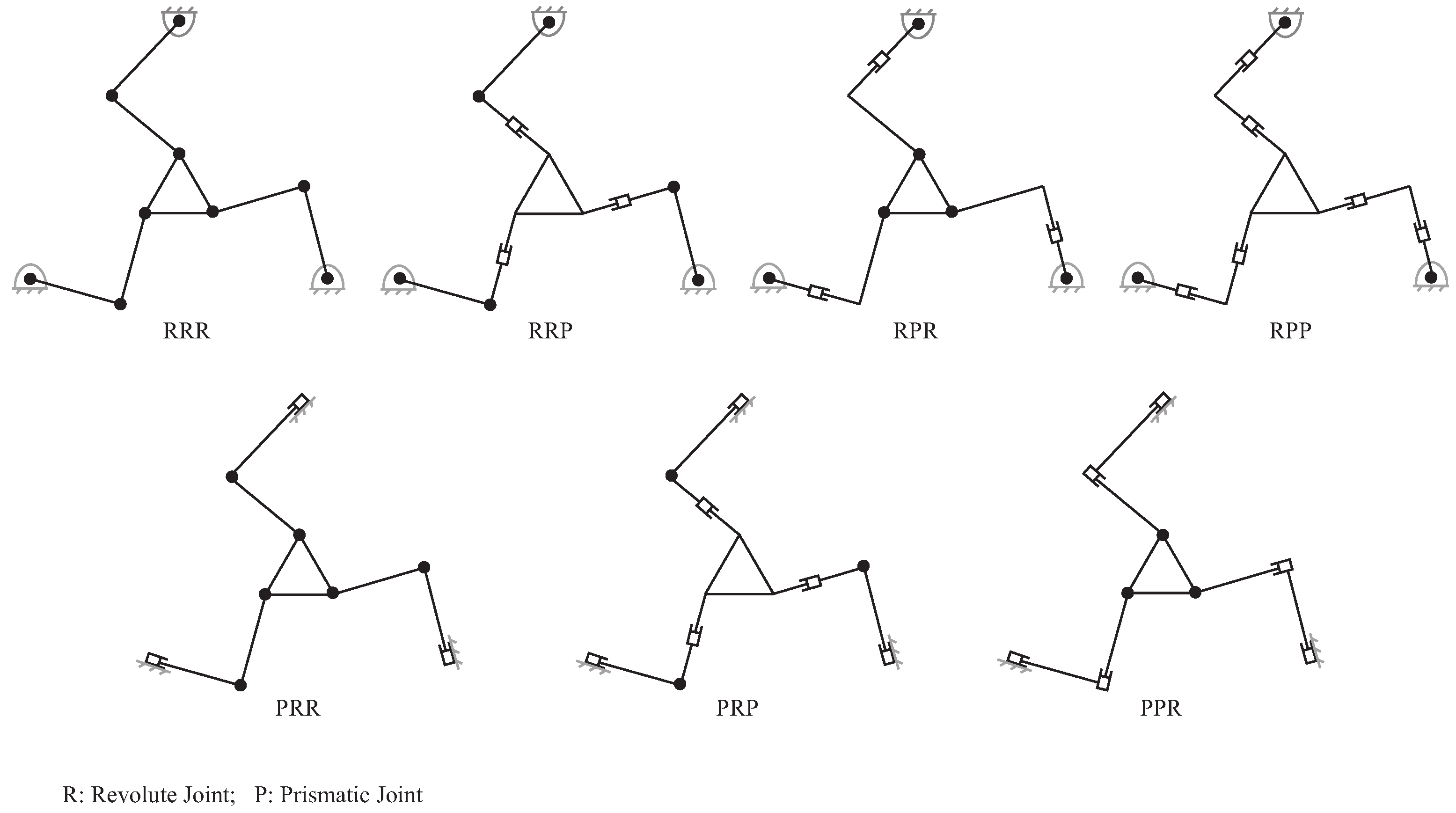
Figure 1. Possible parallel robots configurations.
Symmetry 16 00590 g001
Figure 2. 3RRR symmetric planar robot geometry.
Symmetry 16 00590 g002
Figure 3. Phases of the kinematic model.
Symmetry 16 00590 g003
Figure 4. Planar parallel robot’s mobile platform end-effector [32].
Symmetry 16 00590 g004
Figure 5. First kinematic chain workspace constraint.
Symmetry 16 00590 g005
Figure 6. Planar parallel robot base joint positions.
Symmetry 16 00590 g006
Figure 7. Robot’s workspace constraints due to both the first and second kinematic chain lengths.
Symmetry 16 00590 g007
Figure 8. Robot’s workspace constraints due to all three kinematic chain constraints.
Symmetry 16 00590 g008
Figure 9. Kinematic chain geometry with active joints in A, B, and C.
Symmetry 16 00590 g009
Figure 10. Mobile platform geometry considering ϕ .
Symmetry 16 00590 g010
Figure 11. Optimization of P a and P b .
Symmetry 16 00590 g011
Figure 12. Results of the kinematic model when the orientation is needed.
Symmetry 16 00590 g012
Table 1. Comparison of articulated 3RRR symmetric planar robot study (N/A: is not desribed in the paper).
ReferencesActive JointsDirect KinematicsInverse Kinematics
[3]P, Q, RN/AGeometry Method
[4]P, Q, RN/AScrews theory
[5]P, Q, RGeometry MethodGeometry Method
[6]P, Q, RN/AState Variables
[7]P, Q, RN/AGeometry Method
[8]P, Q, RTransformation matrixGeometry Method
[9]P, Q, RGeometry MethodGeometry Method
[10]P, Q, RN/AGeometry Method
[11]P, Q, RNumeric MethodGeometry Method
[12]P, Q, RN/AGeometry Method
[22]All JointsGeometry MethodN/A
Table 2. Solutions for optimization of P a and P b .
Solution P a P b
#1 b + b 2 4 a c 2 a P y m 2 ( P x P a ) 2
#2 b b 2 4 a c 2 a P y m 2 ( P x P a ) 2
#3 b + b 2 4 a c 2 a P y + m 2 ( P x P a ) 2
#4 b b 2 4 a c 2 a P y + m 2 ( P x P a ) 2
Table 3. θ 1 , θ 2 , and θ 3 obtained from certain parameters, and ϕ is considered.
H P x P y ϕ θ 1 θ 2 θ 1
250125.510121 5 . 08 ° 85 . 34 ° 58 . 76 °
20010010220 10 . 34 ° 69 . 66 ° 60 . 00 °
140707025 8 . 49 ° 71 . 23 ° 54 . 73 °
160604050 31 . 03 ° 117 . 84 ° 36 . 81 °
250403010 44 . 14 ° 159 . 49 ° 105 . 34 °
1904925−10 44 . 34 ° 146 . 23 ° 111 . 89 °
1003550−20 14 . 64 ° 88 . 92 ° 123 . 57 °
110506025 14 . 42 ° 70 . 69 ° 60 . 11 °
95405045 10 . 18 ° 78 . 03 ° 43 . 22 °
81355237 28 . 89 ° 52 . 58 ° 44 . 47 °
Table 4. θ 1 , θ 2 , and θ 3 obtained from certain parameters, and ϕ is not considered.
H P x P y θ 1 θ 2 θ 1
22113035 31 . 35 ° 92 . 84 ° 76 . 42 °
18112035 21 . 45 ° 75 . 42 ° 67 . 71 °
20015950 3 . 28 ° 28 . 34 ° 44.17 . 81 °
21016055 1 . 81 ° 41 . 57 ° 50 . 78 °
1506190 22 . 36 ° 67 . 00 ° 63 . 50 °
1356182 24 . 29 ° 58 . 11 ° 59 . 05 °
1004049 6 . 70 ° 88 . 13 ° 74 . 06 °
1074051.7 6 . 01 ° 92 . 50 ° 76 . 25 °
9365.935.6 7 . 53 ° 41 . 68 ° 50 . 84 °
351100100 19 . 43 ° 128 . 87 ° 94 . 43 °
Table 5. θ 1 , θ 2 , and θ 3 obtained from certain parameters, and ϕ is and is not considered (H = 230).
ϕ Orientated Not Orientated
P x P y ϕ θ 1 θ 2 θ 3 θ 1 θ 2 θ 3
851145° 64 . 96 ° 127 . 35 ° 17 . 39 ° 59 . 44 ° 133 . 63 ° 96 . 81 °
731145° 69 . 28 ° 135 . 55 ° 21 . 27 ° 62 . 21 ° 141 . 57 ° 100 . 78 °
602345° 61 . 6 ° 143 . 59 ° 36.99 ° 52 . 94 ° 147 . 83 ° 103 . 91 °
604145° 43 . 43 ° 139 . 82 ° 51 . 39 ° 36 . 82 ° 142 . 33 ° 101 . 16 °
6010045° 1 . 40 ° 111 . 22 ° 67 . 63 ° 3 . 20 ° 111 . 66 ° 85 . 83 °
9010045° 2 . 91 ° 96 . 225 ° 48 . 31 ° 0 . 76 ° 97 . 55 ° 78 . 77 °
13110045° 1 . 45 ° 65 . 78 ° 22 . 239 ° 2 . 79 ° 69 . 12 ° 64 . 56 °
1659045° 12 . 21 ° 26 . 64 ° 6 . 14 ° 10 . 28 ° 36 . 64 ° 48 . 32 °
1657245° 0 . 63 ° 41 . 51 ° 4 . 12 ° 1 . 43 ° 50 . 02 ° 55 . 01 °
1652245° 25 . 17 ° 56 . 84 ° 13 . 32 ° 26 . 04 ° 67 . 28 ° 63 . 64 °
1151245° 53 . 09 ° 105 . 34 ° 7 . 25 ° 50 . 24 ° 112 . 40 ° 86 . 20 °
1155145° 31 . 25 ° 100 . 29 ° 24 . 03 ° 28 . 38 ° 104 . 59 ° 82 . 29 °
1159245° 6 . 60 ° 83 . 94 ° 32 . 33 ° 4 . 60 ° 86 . 52 ° 73 . 26 °
1179045° 7 . 53 ° 83 . 47 ° 30 . 93 ° 5 . 53 ° 86 . 21 ° 73 . 10 °
9313545° 19 . 17 ° 69 . 16 ° 43 . 33 ° 20 . 39 ° 70 . 07 ° 65 . 03 °
13013045° 22 . 40 ° 40 . 77 ° 18 . 17 ° 22 . 97 ° 44 . 05 ° 52 . 02 °
1306245° 21 . 21 ° 84 . 88 ° 18 . 67 ° 19 . 21 ° 89 . 43 ° 74 . 71 °
911145° 62 . 77 ° 123 . 15 ° 15 . 38 ° 57 . 89 ° 129 . 57 ° 94 . 78 °
11514045° 25 . 58 ° 46 . 31 ° 26 . 90 ° 26 . 45 ° 48 . 29 ° 54 . 14 °
707145° 20 . 13 ° 122 . 57 ° 57 . 43 ° 16 . 57 ° 123 . 96 ° 91 . 98 °
Table 6. Standard deviation of the columns of angles.
Angle Name ϕ OrientationNo Orientation
θ 1 26.0624.67
θ 2 32.4631.62
θ 3 22.3115.81
Disclaimer/Publisher’s Note: The statements, opinions and data contained in all publications are solely those of the individual author(s) and contributor(s) and not of MDPI and/or the editor(s). MDPI and/or the editor(s) disclaim responsibility for any injury to people or property resulting from any ideas, methods, instructions or products referred to in the content.