Practical Prescribed Tracking Control of n-DOF Robotic Manipulator with Uncertainties via Friction Compensation Approach

Abstract

This paper presents a practical and straightforward control strategy for robotic manipulators with unknown dynamics to achieve prescribed tracking performance, which has implementation advantages compared with previous work. In particular, an improved extended state observer (ESO) synthesized with a continuously differentiable friction model and time-varying gains is presented to estimate system states and unknown dynamics. This ESO outperforms the conventional ones in dealing with friction mutations while avoiding peaking estimation values in the initial stage. By combining the prescribed performance function and the proposed ESO, an independent joint control scheme is proposed for a robotic manipulator to keep the tracking error within a predefined performance bound based only on position measurements. The effectiveness of the proposed control scheme is verified by comparative simulation and experimental results on a six-degrees-of-freedom robotic manipulator with active disturbance rejection controller and PID methods.

1. Introduction

1.1. Background and Motivation

Robotic manipulators are crucial in various applications, e.g., industrial automation, medical robotics, and space exploration. The requirements for robotic manipulator control schemes can be categorized into three primary aspects:

(1)

Achieving the control objectives efficiently and precisely.

(2)

Robustness against uncertain dynamics and external disturbances.

(3)

Easy implementation and tuning in engineering practice.

These requirements often involve trade-offs and balancing, and numerous efforts have been devoted to designing robotic manipulator control algorithms [1,2,3,4,5,6,7,8]. Due to the inherent non-linearity and external disturbances of robotic systems, previous advanced control algorithms often employ intricate and exquisite structures to improve system robustness and control accuracy. As a result, the algorithm complexity and parameters grow rapidly with the number of robot links. Meanwhile, practical scenarios rarely provide ideal conditions for the algorithms. Instead, practical robotic systems involve certain constraints, such as limited computational resources and lacking velocity-sensing devices. Designing an easy-to-implement and effective algorithm remains challenging.

Therefore, this paper develops a straightforward and effective control algorithm for robotic systems with multi-degree-of-freedom (DOF) applications, with ease of implementation, robustness, and precision.

1.2. Related Work

The fundamental challenge of controlling a robotic system lies in its strong non-linearity, uncertainties (e.g., payload variation, parameter perturbations, and unmodeled dynamics), and external disturbances. Meanwhile, symmetry is crucial in robotics and must be considered in robot shape and structure designs to achieve balance and stability. However, asymmetry can be introduced by machining defects and external disturbances, affecting robot performance and stability. To enhance control robustness, various control strategies have been proposed, such as adaptive approaches [1,2], robust control [3,4], and neural network-based approaches [5,6]. Though effective, these algorithms are complex, involving too many parameters and requiring velocity feedback. The linear extended state observer (LESO) [9] can overcome these limitations. When applied to a single input single output (SISO) system, LESO effectively estimates the lumped uncertainty and unmeasured velocity state using a quite simple structure with only one parameter [10,11]. Nevertheless, LESO still has the following two limitations:

(1)

It cannot promptly capture abrupt perturbations, such as friction mutations resulting from velocity reversal [12].

(2)

High constant gains may bring peak values if the initial position error is significant.

Despite several improved ESOs based on non-linear structures or parameter optimization [13,14], the construction and stability analysis of practical ESOs remain open questions.

In addition to robustness, control algorithms must also exhibit accuracy. Two types of methods are commonly used to achieve high-accuracy performance: model-based strategies [7,8] and traditional high-gain control algorithms, such as various sliding mode controllers [15,16,17]. However, completely modeling the robot dynamics is laborious, and model-based control strategies are computationally demanding. While sliding mode algorithms can enhance control accuracy, their inevitable chattering limits their application in robotics.

Prescribed performance control (PPC) [18] represents a quantitative approach to predefine tracking transient and steady-state performance. It can be viewed as an advanced high-gain approach guaranteeing tracking accuracy within the predefined control performance. Nonetheless, PPC may exhibit significant short-term errors under large perturbations [19]. Yang et al. [20] and Lin et al. [21] proposed ESO-based PPC approaches for one-link and multi-link robot manipulators, respectively. Still, the effectiveness was only verified through simulations. In addition, limited experimental validation of the performance of ESO-based PPC algorithms for multi-DOF robotic manipulators, particularly six-DOF robotic manipulators, has been reported.

1.3. Contribution and Outline

The main contributions of this study can be summarized as follows:

(1)

A continuously differentiable non-linear friction model is introduced to mitigate the adverse effects of the friction, thereby augmenting observer estimation and overall tracking performance. In addition, a practical way of identifying friction parameters is presented.

(2)

A variable gain finite-time ESO (VGFESO) with friction compensation and time-varying gains is proposed to approximate unknown system dynamics and unmeasured velocities. Compared with the LESO in [20,22], VGFESO significantly attenuates the friction mutation and peaking value influences.

(3)

The composite controller combines the friction model, VGFESO, and a prescribed performance function (PPF) and achieves predefined performance tracking control. Compared with [20,21], the proposed approach has a simpler structure and works under position-measurable conditions alone.

Section 2 covers the problem formulation and preliminary design for a robotic manipulator. Section 3 provides the main results, including the friction model, the controller design procedure, and the stability analysis of the closed-loop system. Numerical simulations and experiments validate the proposed method in Section 4 and Section 5. Section 6 concludes this work.

2. Problem Formulation and Preliminaries

2.1. Dynamic Model and Problem Formulation

The dynamics of an n-link robotic manipulator can be expressed as follows [23]:

$$\begin{array}{c}\hfill M(q)\ddot{q}+C(q,\dot{q})\dot{q}+G(q)+F(\dot{q})=\tau +{\tau }_d\end{array}$$

(1)

where $q,\dot{q},\ddot{q}\in {\mathbb{R}}^n$ are the generalized position, velocity, and acceleration, respectively; inertia matrix $M(q)\in {\mathbb{R}}^{n\times n}$ is symmetric and positive definite; $C(q,\dot{q})\dot{q}\in {\mathbb{R}}^n$ is the centrifugal and Coriolis vector; $G(q)\in {\mathbb{R}}^n$ denotes the gravitational vector; $F(\dot{q})\in {\mathbb{R}}^n$ represents friction torques; ${\tau }_d\in {\mathbb{R}}^n$ is external disturbance; and $\tau \in {\mathbb{R}}^n$ is the input.

Defining $x_1=q\in {\mathbb{R}}^n$, $x_2=\dot{q}\in {\mathbb{R}}^n$, then, (1) can be rewritten into a state-space form:

$$\begin{array}{c}\hfill \left\{\begin{array}{c}{\dot{x}}_1=x_2\hfill \\ {\dot{x}}_2=f-B_0{F}_f(x_2)+B_0\tau \hfill \end{array}\right.\end{array}$$

(2)

where $B_0=diag\{b_{10},\dots ,b_{n0}\}$ ($i=1,2,\dots ,n$); $b_{i0}$ is to be determined; $F_f(·)$ is the continuously differentiable non-linear friction model; and $f\in {\mathbb{R}}^n$ denotes the lumped uncertainty of the robotic system:

$$\begin{array}{c}\hfill f=M^{-1}(q)[\tau -C(q,\dot{q})\dot{q}-G(q)+{\tau }_d-F(\dot{q})]+B_0(F_f-\tau ).\end{array}$$

(3)

Remark 1. 

Equation (3) reveals that the uncertainty term f accounts for all system uncertainties, including modeled approximation errors, unmodeled dynamics, external disturbances, and non-linear couplings among the joints. This approach enables the robot dynamic model to be deconstructed into several subsystems, as expressed in (1).

Assumption 1. 

The joint position $q\in {\mathbb{R}}^n$ is real-time measurable; the desired trajectory $q_d\in {\mathbb{R}}^n$ is in $C^2$ and bounded.

Assumption 2. 

The rate of change of lumped uncertainty f is bounded, i.e., $|\dot{f}|\le L$.

2.2. Error Transformation

We define the tracking error $e(t)=q(t)-q_d(t)$. To satisfy predefined transient and steady-state performance specifications, $e_i(t)$ should be retained within a prescribed bound [18]:

$$\begin{array}{c}\hfill -{\rho }_{i1}{\mu }_i(t)<e_i(t)<{{\rho }_i}_2{\mu }_i(t),\forall t>0\end{array}$$

(4)

where $e_i(t)$ is the i-th element of $e(t)$, ${{\rho }_i}_1>0$, ${{\rho }_i}_2>0$. PPF ${\mu }_i(t)$ can be selected as

$$\begin{array}{c}\hfill {\mu }_i(t)=({{\mu }_i}_0-{{\mu }_i}_{\infty })e^{-l_{i}t}+{{\mu }_i}_{\infty }i=1,\dots ,n\end{array}$$

(5)

where ${{\mu }_i}_0>{{\mu }_i}_{\infty }>0$ and $l_i>0$; ${\mu }_{i\infty }=\underset{t\to \infty }{lim}{\mu }_i(t)>0$ represents the desirable steady-state tracking error; ${{\mu }_i}_0$ is the initial value of ${\mu }_i(t)$, and ${\mu }_i(t)$ is strictly positive, smooth, and exponential-decreasing. As expressed in (4) and (5), ${{\rho }_i}_1{\mu }_i(t)$ and ${{\rho }_i}_2{\mu }_i(t)$ describe the lower and upper bounds of tracking errors, respectively; and $l_i$ represents the convergence rate. Therefore, by selecting ${{\rho }_i}_1$, ${{\rho }_i}_2$, $l_i$, ${{\mu }_i}_0$, and ${{\mu }_i}_{\infty }$, the prescribed performance of tracking error $e_i(t)$ can be determined.

To achieve the prescribed performance for $e_i(t)$, we introduce a smooth and strictly increasing error transformation function $S(z_i)$ of the transformed error $z_i$. $S(z_i)$ transforms (4) into an equivalent “unconstrained” one with the following properties:

Property 1. 

$-{{\rho }_i}_1<S(z_i)<{{\rho }_i}_2$, $\forall z_i\in {L_i}_{\infty }$.

Property 2. 

$\underset{z_i\to +\infty }{lim}S(z_i)={{\rho }_i}_2$, $\underset{z_i\to -\infty }{lim}S(z_i)=-{\rho }_{i1}$.

Based on Properties 1 and 2, (4) can be rewritten as:

$$\begin{array}{c}\hfill e_i(t)={\mu }_i(t)S(z_i).\end{array}$$

(6)

A candidate error transformation function [24] is selected as follows:

$$\begin{array}{c}\hfill S(z_i)=\frac{{\rho }_{i2}{e}^{z_i}-{\rho }_{i1}{e}^{-z_i}}{e^{z_i}+e^{-z_i}}.\end{array}$$

(7)

Based on (6) and (7), $z_i$ can be derived as:

$$\begin{array}{c}\hfill z_i=S^{-1}(\frac{e_i(t)}{{\mu }_i(t)})=\frac{1}{2}ln\frac{{\lambda }_i(t)+{\rho }_{i1}}{{\rho }_{i2}-{\lambda }_i(t)}\end{array}$$

(8)

where ${\lambda }_i(t)=e_i(t)/\phantom{e_i(t){\mu }_i(t)}{\mu }_i(t)$. Then, the derivative of $z_i$ is

$$\begin{array}{c}\hfill {\dot{z}}_i=\frac{\partial S^{-1}}{\partial \lambda }{\dot{\lambda }}_i=r_i({\dot{e}}_i-e_i{{\dot{\mu }}_i/\phantom{{\dot{\mu }}_i\mu }\mu }_i)\end{array}$$

(9)

where $r_i=(1/2{\mu }_i)\left[1/({\lambda }_i+{\rho }_{i1})-1/({\lambda }_i-{\rho }_{i2})\right]$.

Lemma 1 

([24]). The control of system (2) is invariant under the error transform (8) with $S(z_i)$, fulfilling Properties 1 and 2. Therefore, stabilizing $z_i$ is sufficient to guarantee the tracking error of original (2) within prescribed error bound (4).

3. Practical Tracking Control Design

3.1. Continuously Differentiable Friction Model

Designing controllers using discontinuous or piecewise continuous friction models can lead to abrupt changes or instabilities in the control signal at points of discontinuity, making them unsuitable for designing high-performance continuous controllers. Therefore, we use a continuously differentiable friction model [25]:

$$\begin{array}{c}\hfill F_f(\dot{q})={\gamma }_1(tanh({\gamma }_2\dot{q})-tanh({\gamma }_3\dot{q}))+{\gamma }_{4}tanh({\gamma }_5\dot{q})+{\gamma }_6\dot{q}\end{array}$$

(10)

where ${\gamma }_i{|}_{i=1,\dots ,6}>0$ are constants. Model parameter identification is discussed in Section 4.

Remark 2. 

Unlike other friction models, model (10) is continuously differentiable and symmetric about the origin. The stiction coefficients are dominated by ${\gamma }_1$ and ${\gamma }_4$; the Stribeck effect is modeled by $tanh({\gamma }_2\dot{q})-tanh({\gamma }_3\dot{q})$; the Coulomb friction can be approximated by ${\gamma }_{4}tanh({\gamma }_5\dot{q})$; and the viscous dissipation is captured by ${\gamma }_6\dot{q}$. For example, the profile of friction model (10) is shown in Figure 1 when ${\gamma }_1=0.3$, ${\gamma }_2=20$, ${\gamma }_3=1$, ${\gamma }_4=0.3$, ${\gamma }_5=50$, and ${\gamma }_6=0.01$. For a more detailed explanation, see [25].

3.2. VGFESO Design

According to Equation (2), the dynamic model of the i-th link is

$$\begin{array}{c}\hfill \left\{\begin{array}{c}{\dot{x}}_{i1}=x_{i2}\hfill \\ {\dot{x}}_{i2}=f_i-B_{i0}{F}_{if}(x_{i2})+B_{i0}{\tau }_i.\hfill \end{array}\right.\end{array}$$

(11)

Then, we design the observer for each subsystem to estimate the lumped uncertainty and unmeasurable velocity state. Subscript i is omitted for simplicity. We define an augmented state $x_3=f$, and let $h(t)={\dot{x}}_3$, then the subsystem (11) can be re-written as

$$\begin{array}{c}\hfill \left\{\begin{array}{c}{\dot{x}}_1=x_2\hfill \\ {\dot{x}}_2=x_3-b_0{F}_f(x_2)+b_0\tau \hfill \\ {\dot{x}}_3=h.\hfill \end{array}\right.\end{array}$$

(12)

To capture the friction behaviors effectively, friction model (10) is introduced into ESO,

$$\begin{array}{c}\hfill \left\{\begin{array}{c}{\dot{\widehat{x}}}_1={\widehat{x}}_2+{\beta }_1(x_1-{\widehat{x}}_1)\hfill \\ {\dot{\widehat{x}}}_2={\widehat{x}}_3+{\beta }_2(x_1-{\widehat{x}}_1)-b_0{F}_f({\widehat{x}}_2)+b_0\tau \hfill \\ {\dot{\widehat{x}}}_3={\beta }_3(x_1-{\widehat{x}}_1)\hfill \end{array}\right.\end{array}$$

(13)

where ${\widehat{x}}_i$ is the estimation of state $x_i$. According to the poly assignment method [9], ${\beta }_1=3{\omega }_o,{\beta }_2=3{\omega }_o^2,{\beta }_3={\omega }_o^3$, where ${\omega }_o$ denotes the bandwidth of the observer. ESO with constant gains may exhibit peaking values as high-gain observers due to huge initial estimate errors. To tackle this issue, a monotonic increasing function is used to replace ${\omega }_o$ in ${\beta }_i$ as the observer gains, specifically,

$$\begin{array}{c}\hfill \omega (t)=\left\{\begin{array}{cc}{\omega }_0+({\omega }_T-{\omega }_0)·{(\frac{t}{t_L})}^3,& t\le t_L\\ {\omega }_T,& t>t_L.\end{array}\right.\end{array}$$

(14)

The VGFESO with the friction model and time-varying gains can be reconstructed as follows:

$$\begin{array}{c}\hfill \left\{\begin{array}{c}{\dot{\widehat{x}}}_1={\widehat{x}}_2+3\omega (t)(x_1-{\widehat{x}}_1)\hfill \\ {\dot{\widehat{x}}}_2={\widehat{x}}_3+3\omega {(t)}^2(x_1-{\widehat{x}}_1)-b_0{F}_f({\widehat{x}}_2)+b_0\tau \hfill \\ {\dot{\widehat{x}}}_3=\omega {(t)}^3(x_1-{\widehat{x}}_1).\hfill \end{array}\right.\end{array}$$

(15)

We define the state estimation error ${\tilde{x}}_j=x_j-{\widehat{x}}_j,j=1,2,3$. Then, we have the estimation error dynamics as follows:

$$\begin{array}{c}\hfill \left\{\begin{array}{c}{\dot{\tilde{x}}}_1={\tilde{x}}_2-3\omega (t){\tilde{x}}_1\hfill \\ {\dot{\tilde{x}}}_2={\tilde{x}}_3-3\omega {(t)}^2{\tilde{x}}_1+{\tilde{F}}_f\hfill \\ {\dot{\tilde{x}}}_3=h-\omega {(t)}^3{\tilde{x}}_1\hfill \end{array}\right.\end{array}$$

(16)

where ${\tilde{F}}_f=F_f({\widehat{x}}_2)-F_f(x_2)$ is the friction model error. To facilitate the stability analysis, we define a scaled estimation error $\eta ={[{\eta }_1,{\eta }_2,{\eta }_3]}^{\top }$ with ${\eta }_j:={\tilde{x}}_j/\omega {(t)}^{j-1}$, $j=1,2,3$, and

$$\begin{array}{c}\hfill \dot{\eta }=\omega (t)A\eta +\frac{\dot{\omega }(t)}{\omega (t)}B\eta +C\frac{h}{\omega {(t)}^2}+D\frac{1}{\omega (t)}{\tilde{F}}_f\end{array}$$

(17)

where

$$\begin{array}{cc}\hfill A& =\left[\begin{array}{ccc}-3& 1& 0\\ -3& 0& 1\\ -1& 0& 0\end{array}\right],B=\left[\begin{array}{ccc}0& & \\ & 1& \\ & & 2\end{array}\right],\hfill \\ \hfill C& ={\left[\begin{array}{ccc}0& 0& 1\end{array}\right]}^{\top },D={\left[\begin{array}{ccc}0& 1& 0\end{array}\right]}^{\top }.\hfill \end{array}$$

(18)

Then, $\exists P>0$, satisfying:

$$\begin{array}{c}\hfill \begin{array}{cc}\hfill A^{\top }P+PA& \le -I_3,\hfill \\ \hfill B^{\top }P+PB& \ge 0\hfill \end{array}\end{array}$$

(19)

where $I_3$ denotes a three-dimensional identity matrix. Since $F_f(x_2)$ is continuously differentiable, it is globally Lipschitz with respect to $x_2$; thus, there exists a known constant c, such that

$$\begin{array}{c}\hfill |{\tilde{F}}_f|\le c|{\tilde{x}}_2|\le c\omega (t){\parallel \eta \parallel }^2.\end{array}$$

(20)

Assumption 3. 

$h(t)$ is bounded.

Theorem 1. 

Consider the error system (17) and the VGFESO (15). If $\omega (t)\ge 4c\parallel P\parallel$, then the scale estimation error η is uniformly ultimately bounded.

Proof. 

The detailed proof is shown in Appendix A. □

3.3. Controller Design and Stability Analysis

This section proposes the control strategy based on PPF, friction model, and VGFESO via the backstepping method. We use a two-step approach:

Step 1: We choose a virtual control law as

$$\begin{array}{c}\hfill {\alpha }_1=-k_{1}zr+{\dot{q}}_d+e\dot{\mu }/\phantom{\dot{\mu }\mu }\mu \end{array}$$

(21)

where $k_1>0$. Choose a Lyapunov function $V_1=\frac{1}{2}{z}^2$, then

$$\begin{array}{c}\hfill {\dot{V}}_1=zr(x_2-{\dot{q}}_d-e\dot{\mu }/\phantom{\dot{\mu }\mu }\mu ).\end{array}$$

(22)

We define $\epsilon =x_2-{\alpha }_1$, then

$$\begin{array}{c}\hfill \begin{array}{cc}\hfill {\dot{V}}_1& =zr(\epsilon +{\alpha }_1-{\dot{q}}_d-e\dot{\mu }/\phantom{\dot{\mu }\mu }\mu )\hfill \\ \hfill & =zr(\epsilon -k_{1}zr+{\dot{q}}_d+e\dot{\mu }/\phantom{\dot{\mu }\mu }\mu -{\dot{q}}_d-e\dot{\mu }/\phantom{\dot{\mu }\mu }\mu )\hfill \\ \hfill & =-k_1{z}^2{r}^2+z\epsilon r.\hfill \end{array}\end{array}$$

(23)

Therefore, ${\dot{V}}_1=-k_1{z}^2{r}^2\le 0$ can be derived when $\epsilon =0$.

Step 2: The actual control law $\tau$ is determined. Based on (12),

$$\begin{array}{c}\hfill \dot{\epsilon }={\dot{x}}_2-{\dot{\alpha }}_1=x_3-b_0{F}_f({\widehat{x}}_2)+b_0\tau -{\dot{\alpha }}_1.\end{array}$$

(24)

Due to the differentiation of the non-linear function $\mu$, repeated differentiations will trigger an increase in complexity. Therefore, a tracking differentiator (TD) [26] is introduced to approximate ${\dot{\alpha }}_1$, which can be expressed as

$$\begin{array}{c}\hfill \left\{\begin{array}{c}{\dot{r}}_1=r_2\hfill \\ {\dot{r}}_2=-R\mathrm{sgn}(r_1-r(t)+\frac{\left|r_2\right|r_2}{2R})\hfill \end{array}\right.\end{array}$$

(25)

where $r(t)$ is input signal; $r_1,r_2$ are the states of TD; and R is the parameter to be determined. Properly selecting R can ensure precise tracking of $r(t)$ and $\dot{r}(t)$ by $r_1$ and $r_2$, respectively. The performance of TD has been verified in [27]. Since the VGFESO approximates the unknown states $x_2$ and $x_3$, and the TD estimates ${\dot{\alpha }}_1$, we design the actual control law $\tau$ as follows:

$$\begin{array}{c}\hfill \tau =\frac{-{\widehat{x}}_3+{\widehat{\dot{\alpha }}}_1-zr-k_2{\widehat{z}}_2}{b_0}+F_f({\widehat{x}}_2)\end{array}$$

(26)

where $k_2>0$; and $\widehat{\epsilon }={\widehat{x}}_2-{\alpha }_1$.

The following performance theorem is proposed.

Theorem 2. 

For the robotic systems (1), the proposed controller (26), TD (25), and VGFESO (15) can guarantee that the error z and ε are ultimately bounded, and the tracking error e can converge to the region defined by the prescribed performance bound (4).

Proof. 

Define the following Lyapunov function candidate

$$\begin{array}{c}\hfill V_2=V_1+\frac{1}{2}{\epsilon }^2.\end{array}$$

(27)

Then, the time derivative of (27) is

$$\begin{array}{cc}\hfill & {\dot{V}}_2={\dot{V}}_1+\epsilon \dot{\epsilon }\hfill \\ \hfill & =-k_1{r}^2{z}^2+rz\epsilon +\epsilon (x_3-b_0{F}_f({\widehat{x}}_2)+b_0\tau -{\dot{\alpha }}_1).\hfill \end{array}$$

(28)

Noting that $\epsilon =x_2-{\alpha }_1$, then

$$\begin{array}{c}\hfill \widehat{\epsilon }={\widehat{x}}_2-{\alpha }_1=x_2-{\tilde{x}}_2-{\alpha }_1=\epsilon -{\tilde{x}}_2.\end{array}$$

(29)

Defining ${\tilde{\dot{\alpha }}}_1={\widehat{\dot{\alpha }}}_1-{\dot{\alpha }}_1$, we have

$$\begin{array}{cc}\hfill {\dot{V}}_2& =-k_1{r}^2{z}^2+rz\epsilon \hfill \\ \hfill & +\epsilon ({\tilde{x}}_3-rz-k_2\epsilon +k_2{\tilde{x}}_2+b_0{\tilde{F}}_f+{\tilde{\dot{\alpha }}}_1)\hfill \\ \hfill & =-k_1{r}^2{z}^2-k_2{\epsilon }^2+\epsilon {\tilde{x}}_3+k_2\epsilon {\tilde{x}}_2+b_0\epsilon {\tilde{F}}_f+\epsilon {\tilde{\dot{\alpha }}}_1.\hfill \end{array}$$

(30)

Based on Young’s inequality,

$$\begin{array}{c}\hfill \begin{array}{cccc}\hfill b_0\epsilon {\tilde{F}}_f& \le \frac{1}{2}{\epsilon }^2+\frac{1}{2}{b}_0^2{\tilde{F}}_f^2,\hfill & \hfill \epsilon {\tilde{x}}_3& \le \frac{1}{2}{\epsilon }^2+\frac{1}{2}{\tilde{x}}_3^2,\hfill \\ \hfill k_2\epsilon {\tilde{x}}_2& \le \frac{1}{2}{\epsilon }^2+\frac{1}{2}{k}_2^2{\tilde{x}}_2^2,\hfill & \hfill \epsilon {\tilde{\dot{\alpha }}}_1& \le \frac{1}{2}{\epsilon }^2+\frac{1}{2}{\tilde{\dot{\alpha }}}_1^2.\hfill \end{array}\end{array}$$

(31)

We define the upper bound of approximation errors as $\sigma =sup(|{\tilde{F}}_f|,|{\tilde{x}}_2|,|{\tilde{x}}_3|,|{\tilde{\dot{\alpha }}}_1|)$. According to (31), the upper bound of the right-hand side of (30) can be defined as

$$\begin{array}{c}\hfill \begin{array}{cc}\hfill {\dot{V}}_2& \le -k_1{r}^2{z}^2-k_2{\epsilon }^2+2{\epsilon }^2+\frac{1}{2}(b_0^2{\tilde{F}}_f^2+k_2^2{\tilde{x}}_2^2+{\tilde{x}}_3^2+{\tilde{\dot{\alpha }}}_1^2)\hfill \\ \hfill & \le -k_1{r}^2{z}^2-(k_2-2){\epsilon }^2+\frac{1}{2}(b_0^2+k_2^2+2){\sigma }^2\hfill \\ \hfill & \le -2min\{k_1{r}^2,(k_2-2)\}{V}_2+\frac{1}{2}(b_0^2+k_2^2+2){\sigma }^2\hfill \\ \hfill & \le -\phi V_2+\xi \hfill \end{array}\end{array}$$

(32)

where $k_1>0$, $k_2>2$; $\phi =2min\{k_1{r}^2,(k_2-2)\}$; and $\xi =sup(\frac{1}{2}(b_0^2+k_2^2+2){\sigma }^2)$. The solution of (32) is

$$\begin{array}{c}\hfill V_2\le (V_2(0)-\frac{\xi }{\phi })exp(-\phi t)+\frac{\xi }{\phi }.\end{array}$$

(33)

This completes the proof. □

Based on (33) and the definition of $V_2$, the signals z and $\epsilon$ are uniformly bounded. Therefore, the tracking error e remains within the prescribed performance bounds (4) according to Lemma 1 and can be made arbitrarily small by selecting appropriate predefined parameters.

4. Numerical Simulation

This section presents the simulation results. The controller is simulated on a two-link rigid robotic manipulator, and the dynamic model has been detailed in [12].

Table 1. Parameters of the robotic manipulator.

Symbol	Definition	Value
$m_1$, $m_2$	Mass of links 1 and 2	4 kg, 2 kg
$l_1$, $l_2$	Length of links 1 and 2	0.5 m, 0.25 m
$l_{c1}$, $l_{c2}$	Distance to the centers of mass of links 1 and 2	0.25 m, 0.15 m
$I_1$, $I_2$	Inertia tensors of links 1 and 2	1 kg·m2, 0.8 kg·m2
g	Gravity acceleration	9.8 m/s2

provides the parameters. The actual friction torque for each joint is modeled as $F(\dot{q})=0.5(tanh(1000\dot{q})-tanh(60\dot{q}))+2.5tanh(1000\dot{q})+3\dot{q}$.

The predefined trajectory is $q_d={\left[q_{d1},q_{d2}\right]}^{\top }$, where $q_{d1}=q_{d2}=(1-e^{-0.05t})sin(\pi t)$. The control input limits for joints 1 and 2 are $|{\tau }_1{|}_{max}=300$ N·m and $|{\tau }_2{|}_{max}=200$ N·m, respectively. The initial states are $x_1(0)=x_2(0)=0.5$ rad, with other initial values set to zero. ${\tau }_d={\left[0.2sin(t)+0.05sin(200\pi t),0.05sin(200\pi t)\right]}^{\top }$ serves as an external disturbance. To further test the robustness of the proposed method, $m_2$ is increased from 2 kg to 6 kg at $t=3$ s, simulating the process of picking up a load.

The following three controllers are compared:

(1)

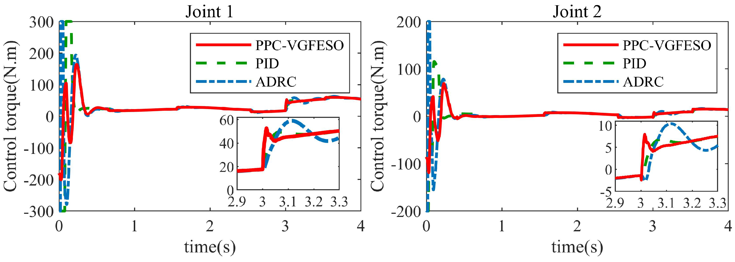
PPC-VGFESO: This is the controller (26) designed in this paper. The PPF parameters are set as ${\mu }_{i0}=0.51$, ${\mu }_{i\infty }=0.005$, $l_i=4$, ${\rho }_{i1}={\rho }_{i2}=1.1$, $i=1,2$. The controller parameters are set as $k_{i1}=0.01$, $k_{i2}=40$, ${\omega }_{i0}=0$, ${\omega }_{iT}=120$, $t_{iL}=0.5s$, $R_i=2000$, $i=1,2$, $b_{10}=0.5$, $b_{20}=1$. The nominal friction model is selected as $F_f(x_2)=0.8F(x_2)$.

(2)

ADRC [22]: The control law can be expressed as

$$\begin{array}{c}\hfill u(t)=\frac{k_p(q_d(t)-{\widehat{x}}_1)+k_v({\dot{q}}_d(t)-{\widehat{x}}_2)+{\ddot{q}}_d-{\widehat{x}}_3}{b_0}\end{array}$$

(34)

where ${\widehat{x}}_i(t)$ is the estimation of state $x_i(t)$ by LESO. The controller parameters are set as $k_{1p}=400$, $k_{1v}=30$, $b_{10}=0.5$, $k_{2p}=324$, $k_{2v}=25$, $b_{20}=1$. To compare with VGFESO, the parameter of LESO is also chosen as ${\omega }_{io}=120$.

(3)

Proportional-integral-derivative (PID): A PID controller is defined as $u=k_{p}e+k_i\int edt+k_d\dot{e}$. Its gains are $k_{1p}=5000$, $k_{1i}=2000$, $k_{1d}=400$, $k_{2p}=2000$, $k_{2i}=1000$, and $k_{2d}=150$, which are adjusted through trial and error to balance steady-state and transient performance.

The simulation results in Figure 2 demonstrate that the proposed controller ensures that the tracking errors of the manipulator remain within prescribed bounds and converge to a small predefined vicinity around the origin. In contrast, the tracking errors for the other two controllers without prescribed performance obviously exceed these bounds. Notably, the system guided by the proposed controller exhibits better robustness against perturbations. With disturbances at $t=3$ s, the system quickly returns to a stable condition with minimal oscillation. This is attributed to the following two factors:

(1)

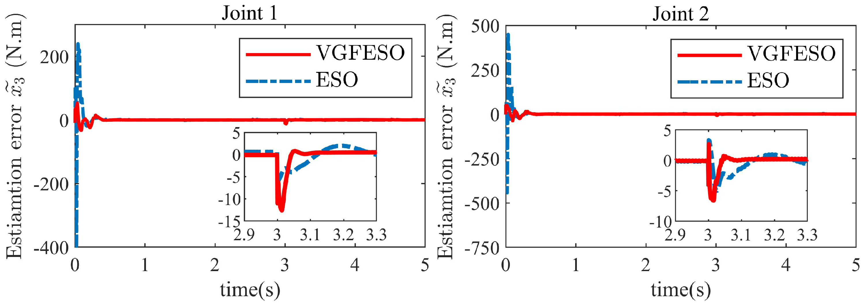
The rapid disturbance estimation by VGFESO and effective compensation, as shown in Figure 3;

(2)

The steady-state performance is strictly constrained by the PPF.

Figure 4 presents the control input signals. It is worth noting that the actuators in PID and ADRC may operate at the upper/lower saturation limits for extended periods or experience more abrupt changes, potentially causing motor damage. The proposed method avoids actuator saturation issues, as VGFESO effectively compensates for uncertainties while the time-varying gains address the peaking value problem.

5. Experiment Verification

The effectiveness of the proposed method is demonstrated on a six-DOF robotic system.

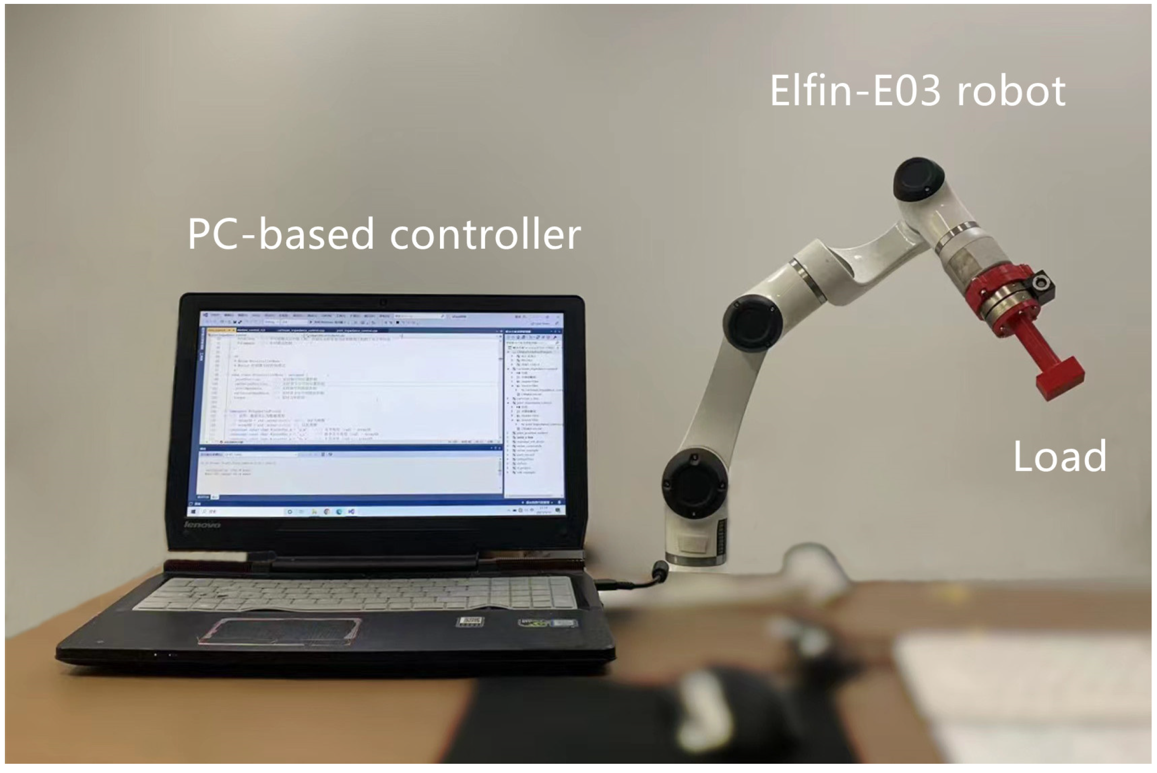
5.1. Experiment Setup

Figure 5 displays the test rig structure, which consists of a collaborative robotic manipulator (Elfin-E03 of Shenzhen Han’s Robot, https://www.hansrobot.net/elfin (accessed on 1 February 2024)), a PC-based motion controller, and monitoring software. This robot has six joints, a 3 kg payload capacity, an operational range of up to 590 mm, and a repeatability accuracy of ±0.02 mm. The gear reduction ratio of the joint reducer is 100, and the encoder has a resolution of 19 bits. The PC-based motion controller developed by our team with Intel(R) Core (TM) i7-6700HQ 2.6 GHz CPU, 8.00 GB RAM and Windows 10 operating system (OS). The proposed PPC-VGFESO and the contrast control strategies are developed in Microsoft Visual Studio 2015 and the Kithara real-time suite (KRTS). As a modular real-time extension software for Windows, KRTS provides a real-time working environment for control software. The robot and controller are connected via an EtherCAT bus.

The experimental system is designed for tracking control of specified joint position references. In this system, the servomotor is operated in torque control mode and the joint tracking error is determined using the rotary encoder. The sampling rate is set to 1 ms, which is significantly faster than the control requirements considered later.

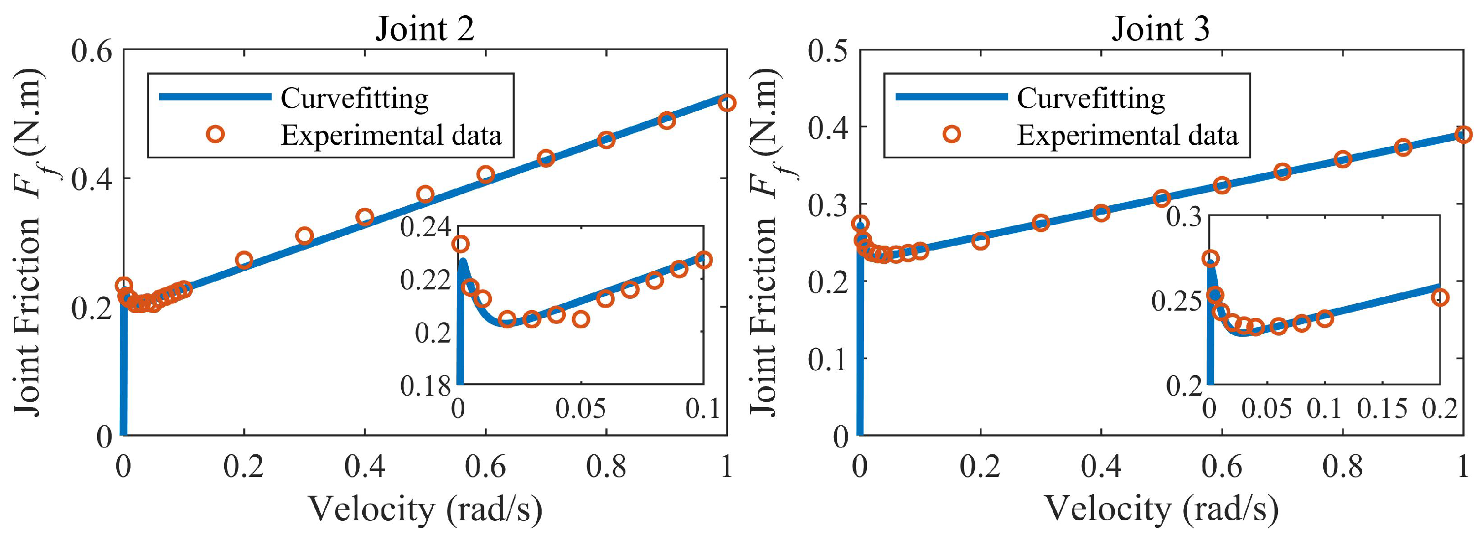
5.2. Friction Parameter Identification

The parameter identification process involves two steps. First, we plot friction forces against corresponding velocities to create a friction–velocity map. The velocities are calculated using backward difference and filtered with a second-order Butterworth low-pass filter [28] to reduce measurement noise. After applying different constant velocities to each joint, a mapping between friction forces and joint velocities is constructed. Second, the friction parameters in (10) are identified using the Differential Evolution (DE) algorithm [29]. Taking joints 2 and 3 as examples, Figure 6 displays the friction–velocity map and friction models identified by DE.

Table 2. Friction parameters of joints 2 and 3 obtained by DE.

Parameters	${\mathit{\gamma }}_1$	${\mathit{\gamma }}_2$	${\mathit{\gamma }}_3$	${\mathit{\gamma }}_4$	${\mathit{\gamma }}_5$	${\mathit{\gamma }}_6$
Joint 2	0.0386	1500	99.0837	0.1970	1500	0.3320
Joint 3	0.0510	1800	79.7978	0.2248	1800	0.1648

lists the corresponding parameters.

5.3. Comparative Experimental Results

This section compares the trajectory tracking performance of three controllers (PPC-VGFESO, ADRC, and PID) in a joint space and Cartesian space.

5.3.1. Trajectory Tracking in Joint Space

We focus on joints 2 and 3, which are most affected by gravity and kinematic coupling.

To test the generality and robustness of the three control methods, control parameters are determined under a given reference trajectory $q_d=0.0873(1-cos(\pi t))$, and remain fixed in all experiments.

Table 3. Control parameters of joints 2 and 3.

Controller	Parameters
PPC-VGFESO	${\mu }_{i0}=0.025, {\mu }_{i\infty }=0.005, l_i=10, {\rho }_{i1}=1, {\rho }_{i2}=1, k_{i1}=1, {\omega }_{i0}=0,$ ${\omega }_{iT}=80, t_{iL}=0.3, R_i=20, d_i=0.001, i=2, 3.k_{22}=30, k_{32}=40$
ADRC	$k_{2p}=361, k_{2v}=38, {\omega }_{2T}=40, b_{20}=0.17, {\omega }_{i0}=0, t_{iL}=0.3, i=2, 3.$ $k_{3p}=576, k_{3v}=48, {\omega }_{3T}=80, b_{30}=0.3$
PID	$k_{2p}=3000, k_{2i}=30, k_{2d}=250, k_{3p}=2800, k_{3i}=20, k_{3d}=200$

lists the parameters. For safety considerations, the time-varying gains in (14) are also used in the ADRC to avoid torque saturation that could damage the actuator.

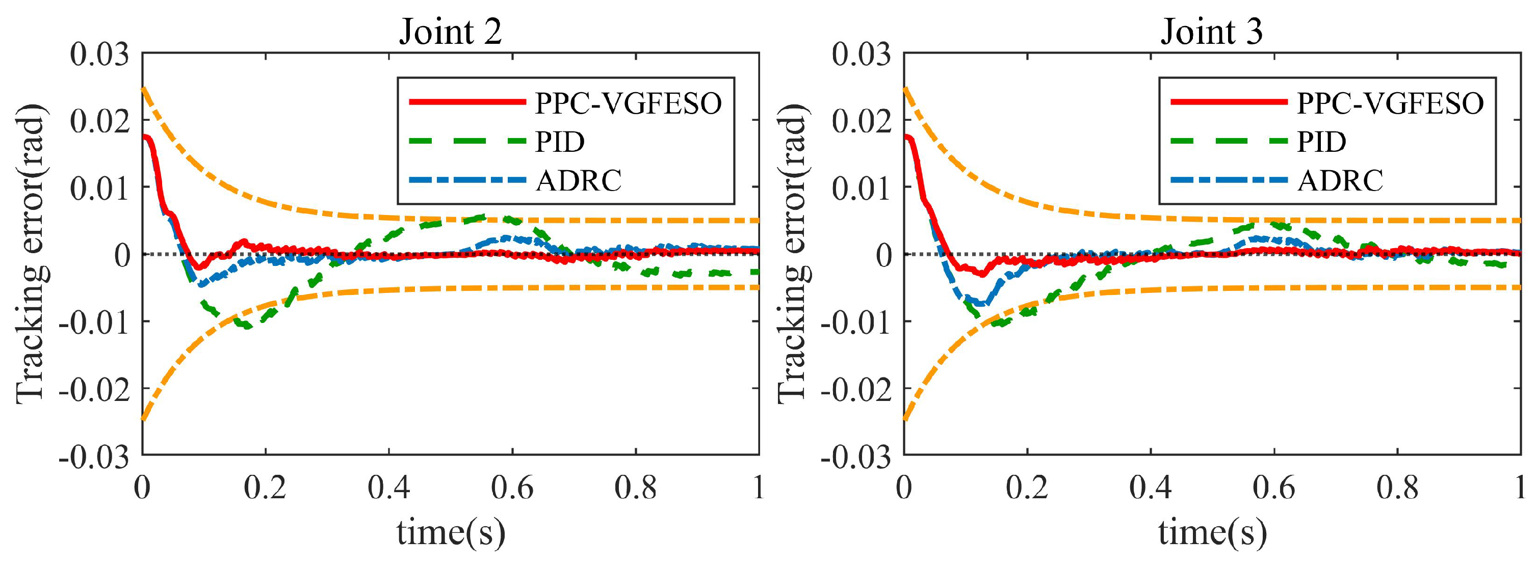
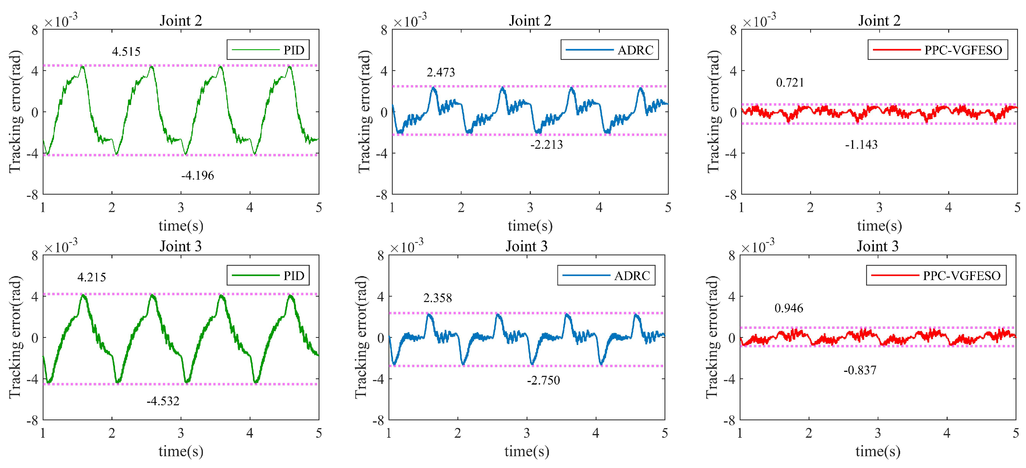
• Case 1—Low-frequency sinusoidal signal tracking and no load: In this experiment, the reference trajectory is $q_d=0.0873(1-cos(\pi t))$, and the robot operates without a load. The initial angular position of each joint is set to 0.0175 rad (1°), and the initial velocity is zero. Figure 7 and Figure 8 present the experimental results. The proposed method exhibits faster convergence and smaller steady-state error than the PID and ADRC controllers. It effectively keeps tracking errors within predefined performance boundaries while successfully addressing abrupt friction changes.
• Case 2—Doubled frequency sinusoidal signal tracking and 1 kg load: A higher frequency sinusoidal trajectory signal $q_d=0.0873(1-cos(2\pi t))$ is employed, with a 1 kg load added to the end. Importantly, the controller parameters remain unchanged from Case 1. The analysis of the experimental results, as shown in Figure 9 and Figure 10, reveals that the proposed PPC-VGFESO maintains satisfactory tracking performance, demonstrating its robustness. In contrast, the overall tracking performance of the PID algorithm deteriorated significantly, while the convergence speed of the ADRC algorithm decreased, accompanied by more pronounced fluctuations in tracking errors. These results highlight the effectiveness of the proposed method.

5.3.2. Trajectory Tracking in Cartesian Space

To validate the trajectory tracking performance of the algorithm in Cartesian space, a square with a side length of 100 mm is selected as the target trajectory in the horizontal XOY plane, maintaining a constant height in the Z direction. The line segment is interpolated using an S-curve, and the target positions in each joint are calculated using inverse kinematics. The end-effector position is obtained by calculating the forward kinematics of the joint positions. We define the end position error of the i-th communication cycle as:

$$\begin{array}{c}\hfill e_i=\sqrt{{(x_i-x_{id})}^2+{(y_i-y_{id})}^2+{(z_i-z_{id})}^2}\end{array}$$

(35)

where $x_{id}$, $y_{id}$, and $z_{id}$ denote the target positions at the i-th cycle; and $x_i$, $y_i$, and $z_i$ denote the actual positions.

To provide convincing results, the performance of the three controllers is compared under different end-effector velocities and loads. The control parameters for the six joints are carefully tuned for the trajectory $q_d=0.0873(1-cos(\pi t))$ and held constant throughout the experiment. Due to space limitations, the parameters are not listed in this paper. Two performance indices are employed, the maximum absolute tracking error $M_e=max|e_i|$ and the average tracking error $A_e=(1/N){\sum }_{i=1}^N|e_i|$, to evaluate the quality of different control algorithms. The following three cases are tested:

• Case 3—Low speed and no load: The velocity of the end effector is set at 300 mm/s, with an acceleration of 600 mm/s² and a jerk of 4000 mm/s³.
• Case 4—Doubled speed and no load: The velocity of the end effector is doubled to 600 mm/s, with an acceleration of 1200 mm/s² and a jerk of 8000 mm/s³.
• Case 5—Doubled speed and 1 kg load: The velocity, acceleration, and jerk remain the same as in Case 4, with a 1 kg load added.

The experimental results are displayed in Figure 11, and the performance indices are summarized in

Table 4. Comparison of performance indices for experimental results.

	300 mm/s, No Load			600 mm/s, No Load			600 mm/s, 1 kg Load
Controller	PID	ADRC	PPC-VGFESO	PID	ADRC	PPC-VGFESO	PID	ADRC	PPC-VGFESO
$M_e$	1.3109	1.0259	0.5168	1.6132	1.4208	0.7996	1.6893	1.5230	0.9948
$A_e$	0.5777	0.4698	0.1797	0.8421	0.7202	0.2472	0.8678	0.7481	0.2725

. It is evident that the proposed PPC-VGFESO outperforms the other two control algorithms in all cases, as indicated by the significantly lower values of $M_e$ and $A_e$. These results demonstrate that the proposed algorithm exhibits excellent tracking control performance and robustness. Furthermore, the fact that the control parameters are adjusted under sinusoidal trajectories highlights the broad applicability of the proposed algorithm.

6. Conclusions

This paper considers a composite control strategy for the trajectory tracking of a rigid n-link robotic manipulator. The strategy combines PPC, VGFESO, and a continuously differentiable friction model to ensure that the transient and steady-state tracking errors of the manipulator remain within the predefined bounds. Specifically, the friction model is employed to compensate for joint non-linear friction, and VGFESO is designed to accurately estimate the unmodeled dynamics and external disturbances of the system. The closed-loop stability of the new controller and observer and the convergence of the tracking error within the predefined bounds are proven using Lyapunov methods. Simulation and extensive comparative experimental results demonstrate the effectiveness of the proposed strategy. With a simple structure, the proposed method can be easily adapted to other types of electromechanical systems, such as biomimetic bat robots. We plan to focus our subsequent research efforts on developing a novel algorithm that incorporates anti-saturation compensation techniques [30] to ensure that the algorithm maintains robust performance even under conditions of actuator saturation.

References

1. Liang, X.; Yao, Z.; Deng, W.; Yao, J. Adaptive control of n-link hydraulic manipulators with gravity and friction identification. Nonlinear Dyn. 2023, 111, 19093–19109. [Google Scholar] [CrossRef]
2. Pezzato, C.; Ferrari, R.; Corbato, C.H. A novel adaptive controller for robot manipulators based on active inference. IEEE Robot. Autom. Lett. 2020, 5, 2973–2980. [Google Scholar] [CrossRef]
3. Xiao, B.; Cao, L.; Xu, S.; Liu, L. Robust tracking control of robot manipulators with actuator faults and joint velocity measurement uncertainty. IEEE/ASME Trans. Mechatron. 2020, 25, 1354–1365. [Google Scholar] [CrossRef]
4. Su, Y.; Zheng, C.; Mercorelli, P. Robust approximate fixed-time tracking control for uncertain robot manipulators. Mech. Syst. Signal. Process. 2020, 135, 106379. [Google Scholar] [CrossRef]
5. Prakash, R.; Behera, L.; Mohan, S.; Jagannathan, S. Dual-Loop Optimal Control of a Robot Manipulator and Its Application in Warehouse Automation. IEEE Trans. Autom. Sci. Eng. 2022, 19, 262–279. [Google Scholar] [CrossRef]
6. Xin, L.; Wang, Y.; Fu, H. Omnidirectional Mobile Robot Dynamic Model Identification by NARX Neural Network and Stability Analysis Using the APLF Method. Symmetry 2020, 12, 1430. [Google Scholar] [CrossRef]
7. Santos, L.; Cortesão, R. Computed-Torque Control for Robotic-Assisted Tele-Echography Based on Perceived Stiffness Estimation. IEEE Trans. Autom. Sci. Eng. 2018, 15, 1337–1354. [Google Scholar] [CrossRef]
8. Gao, J.; Kang, E.; He, W.; Qiao, H. Adaptive model-based dynamic event-triggered output feedback control of a robotic manipulator with disturbance. ISA Trans. 2022, 122, 63–78. [Google Scholar] [CrossRef]
9. Gao, Z. Scaling and bandwidth-parameterization based controller tuning. In Proceedings of the 2003 American Control Conference, Denver, CO, USA, 4–6 June 2003; Volume 6, pp. 4989–4996. [Google Scholar]
10. Patelski, R.; Dutkiewicz, P. On the stability of ADRC for manipulators with modelling uncertainties. ISA Trans. 2020, 102, 295–303. [Google Scholar] [CrossRef]
11. Jin, X.; Lv, H.; He, Z.; Li, Z.; Wang, Z.; Ikiela, N.V.O. Design of Active Disturbance Rejection Controller for Trajectory-Following of Autonomous Ground Electric Vehicles. Symmetry 2023, 15, 1786. [Google Scholar] [CrossRef]
12. Chen, C.; Zhang, C.; Hu, T.; Ni, H.; Luo, W. Model-assisted extended state observer-based computed torque control for trajectory tracking of uncertain robotic manipulator systems. Int. J. Adv. Robot. 2018, 15, 1729881418801738. [Google Scholar] [CrossRef]
13. Ran, M.; Li, J.; Xie, L. A new extended state observer for uncertain nonlinear systems. Automatica 2021, 131, 109772. [Google Scholar] [CrossRef]
14. Zhou, X.; Li, X. Trajectory tracking control for electro-optical tracking system based on fractional-order sliding mode controller with super-twisting extended state observer. ISA Trans. 2021, 117, 85–95. [Google Scholar] [CrossRef] [PubMed]
15. Qian, D.; Zhang, G.; Wang, J.; Wu, Z. Second-Order Sliding Mode Formation Control of Multiple Robots by Extreme Learning Machine. Symmetry 2019, 11, 1444. [Google Scholar] [CrossRef]
16. Chertopolokhov, V.; Andrianova, O.; Hernandez-Sanchez, A.; Mireles, C.; Poznyak, A.; Chairez, I. Averaged sub-gradient integral sliding mode control design for cueing end-effector acceleration of a two-link robotic arm. ISA Trans. 2023, 133, 134–146. [Google Scholar] [CrossRef] [PubMed]
17. Zhang, Z.; Chen, Y.; Wu, Y.; He, B.; Miao, Z.; Zhang, H.; Wang, Y. Hybrid Force/Position Control for Switchable Unmanned Aerial Manipulator Between Free Flight and Contact Operation. IEEE Trans. Autom. Sci. Eng. 2023, 1–15. [Google Scholar] [CrossRef]
18. Bechlioulis, C.P.; Rovithakis, G.A. Robust adaptive control of feedback linearizable MIMO nonlinear systems with prescribed performance. IEEE Trans. Autom. Control 2008, 53, 2090–2099. [Google Scholar] [CrossRef]
19. Zhang, C.; Wu, J.; Ahn, C.K.; Fei, Z.; Wei, C. Learning observer and performance tuning-based robust consensus policy for multiagent systems. IEEE Sens. J. 2021, 16, 431–439. [Google Scholar] [CrossRef]
20. Yang, Y.; Tan, J.; Yue, D. Prescribed performance control of one-DOF link manipulator with uncertainties and input saturation constraint. IEEE/CAA J. Autom. Sin. 2018, 6, 148–157. [Google Scholar] [CrossRef]
21. Ding, Y.; Wang, Y.; Chen, B. Fault-tolerant control of an aerial manipulator with guaranteed tracking performance. Int. J. Robust Nonlinear Control 2022, 32, 960–986. [Google Scholar] [CrossRef]
22. Stanković, M.R.; Manojlović, S.M.; Simić, S.M.; Mitrović, S.T.; Naumović, M.B. FPGA system-level based design of multi-axis ADRC controller. Mechatronics 2016, 40, 146–155. [Google Scholar] [CrossRef]
23. Spong, M.W. An historical perspective on the control of robotic manipulators. Annu. Rev. Control Robot. Auton. Syst. 2022, 5, 1–31. [Google Scholar] [CrossRef]
24. Na, J.; Chen, Q.; Ren, X.; Guo, Y. Adaptive prescribed performance motion control of servo mechanisms with friction compensation. IEEE Trans. Ind. Electron. 2013, 61, 486–494. [Google Scholar] [CrossRef]
25. Makkar, C.; Dixon, W.; Sawyer, W.; Hu, G. A new continuously differentiable friction model for control systems design. In Proceedings of the 2005 IEEE/ASME International Conference on Advanced Intelligent Mechatronics, Monterey, CA, USA, 24–28 July 2005; IEEE: Piscataway, NJ, USA, 2005; pp. 600–605. [Google Scholar]
26. Han, J. From PID to active disturbance rejection control. IEEE Trans. Ind. Electron. 2009, 56, 900–906. [Google Scholar] [CrossRef]
27. Guo, B.; Zhao, Z. On convergence of tracking differentiator. Int. J. Control 2011, 84, 693–701. [Google Scholar] [CrossRef]
28. Yao, J.; Jiao, Z.; Ma, D.; Yan, L. High-accuracy tracking control of hydraulic rotary actuators with modeling uncertainties. IEEE/ASME Trans. Mechatron. 2013, 19, 633–641. [Google Scholar] [CrossRef]
29. Storn, R.; Price, K. Differential evolution-a simple and efficient heuristic for global optimization over continuous spaces. J. Glob. Optim. 1997, 11, 341. [Google Scholar] [CrossRef]
30. Hussain, M.; Rehan, M.; Ahn, C.K.; Tufail, M. Robust antiwindup for one-sided Lipschitz systems subject to input saturation and applications. IEEE Trans. Ind. Electron. 2018, 65, 9706–9716. [Google Scholar] [CrossRef]
31. Qu, Z.; Dawson, D.M.; Lim, S.Y.; Dorsey, J.F. A new class of robust control laws for tracking of robots. Int. J. Rob. Res. 1994, 13, 355–363. [Google Scholar]
Figure 1. Profile of friction model (10).
Symmetry 16 00423 g001
Figure 2. Position tracking errors of joints 1 and 2 for q d = ( 1 e 0.05 t ) sin ( π t ) : (a) Transient tracking error of joint 1; (b) Steady-state tracking error of joint 1; (c) Transient tracking error of joint 2; (d) Steady-state tracking error of joint 2.
Symmetry 16 00423 g002
Figure 3. The disturbance estimation errors of VGFESO and ESO.
Symmetry 16 00423 g003
Figure 4. Control input signals of joints 1 and 2 for q d = ( 1 e 0.05 t ) sin ( π t ) .
Symmetry 16 00423 g004
Figure 5. The experimental platform of a robotic system.
Symmetry 16 00423 g005
Figure 6. Experimental results and curve fitting of non-linear friction.
Symmetry 16 00423 g006
Figure 7. Transient position tracking error comparison for Case 1: q d = 0.0873 ( 1 cos ( π t ) ) and no load.
Symmetry 16 00423 g007
Figure 8. Steady-state position tracking error comparison for Case 1: q d = 0.0873 ( 1 cos ( π t ) ) and no load.
Symmetry 16 00423 g008
Figure 9. Transient position tracking error comparison for Case 2: q d = 0.0873 ( 1 cos ( 2 π t ) ) and 1 kg load.
Symmetry 16 00423 g009
Figure 10. Steady-state position tracking error comparison for Case 2: q d = 0.0873 ( 1 cos ( 2 π t ) ) and 1 kg load.
Symmetry 16 00423 g010
Figure 11. Position tracking errors at different end-effector speeds and loads in Cartesian space: (a) Case 3: 300 mm/s and no load; (b) Case 4: 600 mm/s and no load; (c) Case 5: 600 mm/s and 1 kg load.
Symmetry 16 00423 g011