A Symmetric Kernel Smoothing Estimation of the Time-Varying Coefficient for Medical Costs

Abstract

In longitudinal studies, subjects are repeatedly observed at a set of distinct time points until the terminal event time. The time-varying coefficient model extends the parametric method and captures the dynamic trajectories of time-dependent covariate effects, thus enabling it to describe the potential relationship between the longitudinal variable and the observed time points. In this study, we propose a novel approach to the estimation of medical costs using a symmetric kernel smoothing method in the time-varying coefficient joint model. A smooth function of medical costs is derived by weighting the values of longitudinal data at all distinct observed time points via the combination of the kernel method and the inverse probability weighting method. For the simulation study, we first set up the true functions of time-varying coefficients; we then generated random samples for covariates and censored survival times. Subsequently, the longitudinal data of response variables could be produced. Further, numerical simulation experiments were conducted by using the proposed method and applying R code to the generated data. The estimated results for the parameters and non-parametric functions were compared with different settings. The numerical results illustrate that as the sample size increases, the bias and model-based standard errors decrease, and the performance improves with larger sample sizes. The estimates of functions in the model almost coincide with the true functions, as shown in the figures of the simulation study. Furthermore, the consistency of the obtained estimator is demonstrated via theoretical analysis, and a numerical simulation is performed to illustrate the performance of the proposed estimators. The proposed model is applied to a real-world data set acquired from a multicenter automatic defibrillator implantation trial (MADIT).

1. Introduction

In medical cost studies, researchers need to use appropriate methods to evaluate the average medical cost of a patient across their whole life. Due to censoring mechanisms, the survival function is generally not identifiable. Bang and Tsiatis [1] introduced a class of weighted estimators that appropriately account for censoring; although extensive simulation studies showed that the estimators perform well in finite samples, even with heavily censored data, the estimator is not efficient, and the computations are complex. Lin et al. [2] partitioned the entire time period of interest into a number of small intervals and estimated the average total cost to minimize the bias induced by censoring. Furthermore, the estimators were proven to be asymptotically normal. Huang and Lovato [3] formulated weighted log-rank statistics in a marked point process framework and developed the asymptotic theory. The above methods have been applied to estimate the cumulative mean function. However, in addition to censoring mechanisms, data often consist of longitudinal outcomes, time-dependent/independent covariates, event times, and censoring times. In longitudinal studies, subjects are repeatedly observed at a set of distinct time points until the terminal event time. The joint model [4] contains both a longitudinal sub-model, to express the effect on longitudinal measurements from time-dependent covariates, and a survival sub-model, to reveal the survival function association with the longitudinal part. Time-independent covariates are generally present in the survival sub-model due to the absence of repeated measurements.

Deng [5] considered a linear parametric regression model to describe longitudinal data and used the joint modeling technique and the inverse probability weighting method [6] to estimate the cumulative mean function. Although this method can also solve the problem of handling time-dependent covariates and right-censored time-to-event data, it may still be restrictive for capturing initial data.The main reason for this is that the effects of covariates on longitudinal outcomes are considered time-independent constants.

Thus, some researchers have focused on non-parametric longitudinal sub-models (e.g., Hoover et al. [7]; Zhao et al. [8]; Li et al. [9]; Do et al. [10]). There have been numerous approaches to estimating non-parametric estimators in the recent literature, such as kernel, smoothing spline, regression spline, and wavelet-based methods. For instance, Eubank and Speckman [11] proposed a well-behaved non-parametric kernel regression model in a small-sample study with bias-corrected confidence bands and proved the asymptotic properties. Wu et al. [12] minimized the local square criterion and obtained the asymptotic distributions for kernel estimators. However, when the covariate dimension is too high, the smooth estimation of general multivariate non-parametric regression may require a large sample size, and the smoothing results may be difficult to interpret.

Several time-varying coefficient longitudinal models have been considered in recent studies. For instance, You et al. [13] considered the time-varying coefficient as a polynomial basis regression spline, proposed a mixed-effects model for multiple longitudinal outcomes using the local polynomial method, and provided tuning parameters and variable selection. However, this model can only be used in continuous longitudinal outcomes. Observed data tend to be discrete in many applications. Moreover, time-independent covariates were not considered in their study [13]. The joint model with kernel smoothing varying coefficients in the longitudinal sub-model can be used to estimate the cumulative mean function with discrete data. Therefore, in this study, we estimate the cumulative mean function with time-dependent/independent covariates using the kernel method in a joint time-varying coefficient model based on right/interval censoring history process data. In our method, the estimator of the mean state function is unbiased at time points where all subjects are observed. The reason for this is that, after smoothing the function with the kernel method, the values of the original sample points are not changed. Thus, we can utilize all the known information for estimation without data bias. Moreover, in our simulation study, the estimator of the cumulative mean state function is almost equal to the value of the preassigned function at any time point.

The remainder of the paper is organized as follows: Section 2 establishes the joint varying coefficient model and proposes the estimators of time-varying coefficients based on our method. Section 3 demonstrates the feasibility of this method through numerical simulations. Section 4 applies the proposed model to a real-world data set from a multicenter automatic defibrillator implantation trial (MADIT). Section 5 discusses the influence of bandwidth h selection and concludes this paper. Finally, the appendices provide the proofs of the main results.

2. Estimation for a Time-Varing Coefficient Model

It is assumed that history process data are right-censored. Let T denote the terminal event time, and C denote the censoring event time. Let $Y\left(t\right)$ denote the state process which is related to the time-dependent covariate $\mathit{X}\left(t\right)$ and time-independent covariate $\mathit{W}$. The state process satisfies $Y\left(t\right)=0$ when $t⩾T$. For $i=1,2,\dots ,m$, let $T_i$ and $C_i$ denote the true values of T and C for the ith subject. Further, ${\delta }_i=I(T_i⩽C_i)$ denotes the censoring indicator. Assume that censoring time is independent of terminal event time and the state process. Let $y_i\left(t\right)$, q-dimensional vector ${\mathit{x}}_i\left(t\right)={(x_{i1}\left(t\right),x_{i2}\left(t\right),\dots ,x_{iq}\left(t\right))}^T$, and p-dimensional vector ${\mathit{w}}_i={(w_{i1},\dots ,w_{ip})}^T$ be the observed history of $Y\left(t\right)$, $\mathit{X}\left(t\right)$, and $\mathit{W}$ for the ith subject.

Now, the time-varying coefficient joint model can be formed as follows:

$$\left\{\begin{array}{c}{y}_i\left(t\right)={\mathit{x}}_i{\left(t\right)}^T\mathit{\beta }\left(t\right)+{ϵ}_i\left(t\right),\hfill \\ h_i\left(t\right)=h_0\left(t\right)exp\{w_i\gamma +\alpha (y_i\left(t\right)-{ϵ}_i\left(t\right))\},\hfill \end{array}\right.$$

(1)

where $\mathit{\beta }\left(t\right)$ is time-varying coefficient parameter, $\alpha$ is the association coefficient of the longitudinal outcome to the hazards for occurring event, $h_0\left(t\right)$ is the baseline hazards function, which is known in our model, and ${ϵ}_i\left(t\right)$ is the random error with ${ϵ}_i\left(t\right)\sim N(0,{\sigma }^2)$. Further, it is assumed that $ϵ\left(t\right)$ is independent of terminal event T conditional on $X\left(t\right)$ and W.

2.1. Estimation of Time-Varying Coefficient in Longitudinal Model

We should notice that the observations for ith subject $(i=1,2,\dots ,m)$ are not continuous but only able to be obtained at some special times $t_{ij}$, $(j=1,2,\dots ,n_i)$. The state process $Y\left(t\right)$ can be the observed until the event time $T_i^{*}=min(T_i,C_i)$ Thus, let ${\mathit{y}}_i\left(t_{ij}\right)$ be the observed state history. For the sake of illustration, assume ${\mathit{y}}_i\left(t_{ij}\right)=0$ when $t⩾T^{*}$.

For convenience, define sets ${\Delta }_i=\{t_{ij},j=1,2,\dots ,n_i\}$ for $i=1,2,\dots ,m$ and $\Delta =\{t_{\left(k\right)};k=0,1,2,\dots ,N\}$, where $0=t_{\left(0\right)}<t_{\left(1\right)}<t_{\left(2\right)}<\dots <t_{\left(N\right)}$ are the observed distinct time points for all subjects. N denotes the number of all the distinct observed time points.

The estimator $\widehat{\mathit{\beta }}\left(t\right)$ of the time-varying coefficient $\mathit{\beta }\left(t\right)$ can be calculated by minimizing the following equation:

$$L_N\left(t\right)=\sum _{k=1}^N{W}_{k,h}(t-t_{\left(k\right)})\left\{\sum _{i=1}^m{\left[I\{T_i^{*}⩾t_{\left(k\right)}\}\{y_i\left(t_{\left(k\right)}\right)-{\mathit{x}}_i{\left(t_{\left(k\right)}\right)}^T\mathit{\beta }\left(t\right)\}\right]}^2\right\},$$

(2)

where

$$W_{k,h}(t-t_{\left(k\right)})=\frac{K_h(t-t_{\left(k\right)})}{{\sum }_{k=1}^N{K}_h(t-t_{\left(k\right)})},$$

$K_h(·)$ is the kernel weight function. The bandwidth, which is generally selected according to the observed time points, reveals the distance of t and $t_{\left(k\right)}$. There is a major distinction between the estimation from Equation (2) and the estimation in Wu [12] since the censoring mechanism, indicator $I\{T_i^{*}⩾t_{\left(k\right)}\}$, is necessary in order to avoid incomplete data due to censoring.

Remark 1. 

We assume that $K_h(·)$ is the Epanechnikov kernel function. The cross-validation method can be used to select the appropriate kernel function. The kernel function with the smallest induced error is considered the best. More details on kernel function selection can be found in [14].

Equivalently, we write Equation (2) in the matrix form:

$$L_N\left(t\right)=\sum _{k=1}^N{\left({\mathbf{Y}}_k-{\mathbf{X}}_k\mathit{\beta }\left(t\right)\right)}^T{\tilde{\mathbf{D}}}_k\left(t\right)\left({\mathbf{Y}}_k-{\mathbf{X}}_k\mathit{\beta }\left(t\right)\right),$$

(3)

where

$${\mathbf{Y}}_k=\left(\begin{array}{c}{y}_1\left(t_{\left(k\right)}\right)\\ ⋮\\ y_m\left(t_{\left(k\right)}\right)\end{array}\right),$$

$${\mathbf{X}}_k=\left(\begin{array}{ccc}{x}_{11}\left(t_{\left(k\right)}\right)& \cdots & x_{1q}\left(t_{\left(k\right)}\right)\\ ⋮& \cdots & ⋮\\ x_{m1}\left(t_{\left(k\right)}\right)& \cdots & x_{mq}\left(t_{\left(k\right)}\right)\end{array}\right),$$

and

$${\tilde{\mathbf{D}}}_k\left(t\right)=\mathrm{diag}\left(W_{k,h}(t-t_{\left(k\right)})I\{T_1^{*}⩾t_{\left(k\right)}\},\dots ,W_{k,h}(t-t_{\left(k\right)})I\{T_m^{*}⩾t_{\left(k\right)})\right),$$

It is assumed that $\left({\sum }_{k=1}^N{\mathbf{X}}_{t_{\left(k\right)}}^T{\tilde{\mathbf{D}}}_k{\mathbf{X}}_{t_{\left(k\right)}}\right)$ is also invertible. By minimizing Equation (3), $\widehat{\mathit{\beta }}\left(t\right)$ can be expressed as the following q-dimensional column vector:

$$\widehat{\mathit{\beta }}\left(t\right)={\left(\sum _{k=1}^N{\mathbf{X}}_k^T{\tilde{\mathbf{D}}}_k\left(t\right){\mathbf{X}}_k\right)}^{-1}\left(\sum _{k=1}^N{\mathbf{X}}_k^T{\tilde{\mathbf{D}}}_k\left(t\right){\mathbf{Y}}_k\right).$$

(4)

The traditional method for bandwidth selection is K-fold cross-validation (CV). Time-varying coefficients complicate the calculation. However, ‘leave-one-subject-out’ cross-validation proposed by Rice and Sliverman [15] can be used in such scenarios. In this case, the kernel weight function is $K(t-t_{\left(k\right)};h)$, the estimator of time-varying coefficient $\mathit{\beta }\left(t\right)$ is $\widehat{\mathit{\beta }}(t;h)$. Minimizing the following equation:

$$CV\left(h\right)=\sum _{k=1}^N\sum _{i=1}^{m}E{\left[I\{T_i^{*}⩾t_{\left(k\right)}\}\{y_i\left(t_{\left(k\right)}\right)-{\mathit{x}}_i{\left(t_{\left(k\right)}\right)}^T{\mathit{\beta }}^{(-i)}(t_{\left(k\right)};h)\}\right]}^2,$$

where ${\widehat{\mathit{\beta }}}^{(-i)}(t_{\left(k\right)};h)$ is the kernel estimator computed with all measurements except the measurements of ith subject. Then, the cross-validation bandwidth can be obtained.

2.2. Estimation of Survival Model

Define $m_i\left(t\right)=y_i\left(t\right)-{ϵ}_i\left(t\right)={\mathit{x}}_i{\left(t\right)}^T\mathit{\beta }\left(t\right)$, and then the estimate of $m_i\left(t\right)$ is

$${\widehat{m}}_i\left(t\right)={\mathit{x}}_i{\left(t\right)}^T\widehat{\mathit{\beta }}\left(t\right).$$

The data related to survival sub-model consist of $\{({\mathit{x}}_i\left(t\right),{\mathit{w}}_{\mathit{i}},T_i^{*},{\delta }_i,);i=1,2,\dots ,m\}$.

For each given $t\in R$,

$$h_i\left(t\right)=h_0\left(t\right)exp\{{\mathit{w}}_i\gamma +\alpha m_i\left(t\right)\},$$

The Cox partial maximum likelihood function [4] is

$$L_p(\gamma ,\alpha )=\prod _{i=1}^m{\left[\frac{exp\{{\mathit{w}}_i\gamma +\alpha m_i\left(T_i^{*}\right)\}}{{\int }_0^{T_i^{*}}exp\{{\mathit{w}}_i\gamma +\alpha m_i\left(s\right)\}ds}\right]}^{{\delta }_i}.$$

(5)

The log-partial likelihood function for Equation (5) is

$$\begin{array}{cc}\hfill LL\left(\mathit{\theta }\right)& =log{L}_p(\gamma ,\alpha )\hfill \\ \hfill & =\sum _{i=1}^m{\delta }_i\left[{\mathit{w}}_i\gamma +\alpha \left(m_i\left(T_i^{*}\right)\right)-log{\int }_0^{T_i^{*}}exp\{{\mathit{w}}_i\gamma +\alpha m_i\left(s\right)\}ds\right].\hfill \end{array}$$

(6)

Then, replacing $m_i\left(t\right)$ by the estimator ${\widehat{m}}_i\left(t\right)$, the estimator $\widehat{\mathit{\theta }}=(\widehat{\gamma },\widehat{\alpha })$ can be obtained by maximizing Equation (6).

We define the survival function of T as:

$$S_T\left(t\right)=P(T>t).$$

The estimate of $S_T\left(t\right)$ can be obtained from the hazards function in joint model:

$${\widehat{S}}_T\left(t\right)=exp\left\{-{\int }_0^t{h}_0\left(s\right)exp\{{\mathit{w}}^T\widehat{\gamma }+\widehat{\alpha }\widehat{m}\left(s\right)\}ds\right\}.$$

Theoretically, the estimate ${\widehat{S}}_T\left(t\right)$ is related to the values of covariates $\mathit{x}\left(s\right)$ for $s\in [0,t]$. Since $\mathit{x}\left(t\right)$ generally is not continuously observed, the estimate ${\widehat{S}}_T\left(t\right)$ can not be derived even at observed time points. ${\widehat{S}}_T\left(t\right)$ can be calculated only if $\mathit{x}\left(t\right)$ can be observed continuously. Thus, we replace ${\widehat{S}}_T\left(t\right)$ with the Kaplan–Meier estimator [16]. Alternatively, in terms of the law of large numbers, the survival function can also be estimated as follows:

$$\widehat{S}\left(t\right)=\frac{1}{m}\sum _{i=1}^{m}I\{T_i⩾t\}.$$

(7)

Moreover, the estimate of the survival function of ${\widehat{S}}^{*}\left(t\right)=P(T^{*}>t)$ for $T^{*}$ can be obtained in a similar way.

2.3. Estimation of Cumulative Mean State Function

Suppose $\nu \left(t\right)$ is the mean function of $Y\left(t\right)$, that is, given $X\left(t\right)$, $\nu \left(t\right)=E\left(Y\left(t\right)\mid X\left(t\right)\right)$. Because of the censoring, the proposed estimator $\widehat{\nu }\left(t\right)$ for the mean state function $\nu \left(t\right)$ at any time is as follows:

$$\widehat{\nu }\left(t\right)=\frac{\frac{1}{m}{\sum }_{i=1}^{m}I\{T_i^{*}⩾t\}{\widehat{Y}}_i\left(t\right)}{{\widehat{S}}^{*}\left(t\right)},$$

(8)

where ${\widehat{Y}}_i\left(t\right)={\mathit{x}}_i\left(t\right)\widehat{\mathit{\beta }}\left(t\right)$ is the fitted value of $Y_i\left(t\right)$ at time point t.

Then, the cumulative mean function $\mu \left(t\right)$ for any time point t can be obtained as:

$$\widehat{\mu }\left(t\right)={\int }_0^t\widehat{\nu }\left(s\right)ds.$$

(9)

2.4. The Asymptotic Property of Estimators

Here, we discuss the asymptotic property of estimators. To rigorously define the statements, we introduce various notations. Let $\mathcal{R}\left(t\right)$ denote the observed covariate processes, such as baseline information, study time, and so on, that is, $\mathcal{R}\left(t\right)=\left\{\mathit{x}\right(t),\mathit{w}\}$. Then, let ${\overline{Z}}_{\mathcal{R}}\left(t\right)$ denote the longitudinal covariate history prior to time t and ${\overline{Z}}_Y\left(t\right)$ denote the response history prior to time t, that is, ${\overline{Z}}_{\mathcal{R}}\left(t\right)=\{\mathcal{R}\left(s\right):s<t\}$ and ${\overline{Z}}_Y\left(t\right)=\{Y\left(s\right):s<t\}$. Furthermore, we use $\Vert ·\Vert$ to denote the Euclidean norm in real space and ${\mathcal{R}}^{\prime }\left(t\right)$ to denote the derivative of $\mathcal{R}\left(t\right)$ with respect to time t. It is assumed that all observed time points $t_{ij}$ are independent of each other and follow a distribution $F_T$ with density $f_T$.

Assumption 1. 

$X\left(t\right)$ is Lipschitz-continuous with order ${\lambda }_0$, $|E\left(X_l^T{X}_l\right)-E\left(X_s^T{X}_s\right)|⩽C_0{|t_{\left(l\right)}-t_{\left(s\right)}|}^{{\lambda }_0}$ for any $t_{\left(l\right)}$ and $t_{\left(s\right)}$ in support of $f_T$ and some $C_0>0$, and $\mathit{\beta }\left(t\right)$ and $f_T$ are Lipschitz-continuous with orders of ${\lambda }_1>0$ and ${\lambda }_2>0$, respectively.

Assumption 2. 

$o\left(t\right)={lim}_{\Delta t\to 0}E\left\{ϵ(t+\Delta t)ϵ\left(t\right)\right\}$ and $w\left(t\right)=E\left\{{ϵ}^2\left(t\right)\right\}$ are continuous.

Assumption 3. 

$W_{k,h}(·)$ is square-integrable that integrates to one and satisfies $\int u{W}_{k,h}\left(u\right)du=0$, $m_1=\int u^2{W}_{k,h}\left(u\right)du<\infty$, and $m_2=\int W_{k,h}^2\left(u\right)du<\infty$, while $h\to 0$ and $Nh\to \infty$ as $N\to \infty$.

Assumption 4. 

The bandwidth satisfies $h=N^{-1/5}{M}_0$ for some constant $M_0$.

Assumption 5. 

${lim}_{n\to \infty }{N}^{-6/5}{\sum }_{i=1}^n{n}_i=U$ for some $0⩽U<\infty$

Theorem 1. 

Under Assumptions (1)–(5), the estimator $\widehat{\mathit{\beta }}\left(\tau \right)$ defined in Equation (4) is asymptotically multivariate normal for any $\tau \in [0,T]$ as $m\to \infty$.

We summarize the asymptotic normality of $\widehat{\mathit{\beta }}\left(\tau \right)$ at a fixed point $\tau$, where $\tau \in R$ in Appendix A.

Remark 2. 

Most assumptions are similar regularity conditions as that in Wu et al. [12]. Assumptions 1 and 2 are rigorous statements for which $\left({\sum }_{k=1}^N{\mathbf{X}}_{t_{\left(k\right)}}^T{\tilde{\mathbf{D}}}_k{\mathbf{X}}_{t_{\left(k\right)}}\right)$ is positive-definite and invertible asymptotically. Assumption 3 ensures that $W_{k,h}(·)$ has a compact support on R. Assumptions 4 and 5 are results from finite moments in Assumptions 1 and 2. More discussions about the asymptotic risk for the kernel estimators can be found in [12].

Theorem 2. 

It is assumed that for $t\in (0,T)$, $E(y_i\left(t\right)\mid {\mathit{x}}_i\left(t\right))=E(Y\left(t\right)\mid \mathbf{X}\left(t\right))$, the estimator $\widehat{\nu }\left(t\right)$ defined in Equation (8) is an unbiased estimator for any $t\in \Delta$.

The proof can be found in Appendix B.

Based on Zeng and Cai [17], the following assumptions are imposed on the joint model.

Assumption 6. 

For any $t\in [0,T]$, the covariate process $\mathcal{R}\left(t\right)$ is fully observed and conditional on ${\overline{Z}}_{\mathcal{R}}\left(t\right)$, ${\overline{Z}}_Y\left(t\right)$, and $T⩾t$; the distribution of $\mathcal{R}\left(t\right)$ depends only on ${\overline{Z}}_{\mathcal{R}}\left(t\right)$. $\mathcal{R}\left(t\right)$ is continuously differentiable in $[0,T]$ and $ma{x}_{t\in [0,T]}\Vert {\mathcal{R}}^{\prime }\left(t\right)\Vert <\infty$ with a probability of one.

Assumption 7. 

The censoring time C depends only on ${\overline{Z}}_{\mathcal{R}}\left(t\right)$ and $\mathcal{R}\left(t\right)$ for any $t<T$ conditional on ${\overline{Z}}_{\mathcal{R}}\left(t\right)$, ${\overline{Z}}_Y\left(t\right)$, $\mathcal{R}\left(t\right)$ and $T⩾t$.

Assumption 8. 

Full-rank $P({\mathit{X}}^T\mathit{X}$ ) is positive. Additionally, if there is an existing constant vector ${\mathit{C}}_0$ satisfying $\mathit{X}{\left(t\right)}^T{\mathit{C}}_0=g\left(t\right)$ for a deterministic function $g\left(t\right)$ for all $t\in [0,T]$ with a positive probability, then ${\mathit{C}}_0=0$ and $g\left(t\right)=0$.

Assumption 9. 

The true value of parameter $\mathit{\theta }=\left({\sigma }^2,{\gamma }^T,\alpha \right)$ satisfies $\Vert \theta \Vert ⩽Q_0,{\sigma }_0^2>Q_0^{-1}$ for a known positive constant $Q_0$.

Assumption 10. 

The baseline hazard function $h_0\left(t\right)$ is bounded and positive in $[0,T]$.

Assumption 11. 

There is an existing positive constant $a>0$ satisfying $S_T\left(T\right)⩾a$.

Remark 3. 

Assumption 6 serves as a fundamental statement in joint models, indicating that the association between the history process and the survival time is due to observed covariate processes, such as baseline information, study time, and so on, denoted by $\mathcal{R}\left(t\right)$. Assumption 7 means that there exist some appropriate measures such that the intensity function of $Nc\left(t\right)$ exists. Assumption 8 is the identifiability assumption in a linear mixed-effects model. Assumptions 9–11 imply that, conditional on ${\overline{Z}}_{\mathcal{R}}\left(t\right)$ and $\mathcal{R}\left(t\right)$, the probability of a subject surviving after time τ is at least some positive constant. Theorem 3.1 in Zeng and Cai [17] states the strong consistency of the maximum likelihood estimator. More discussions on the assumptions can be found in [17].

Theorem 3. 

Under Assumptions (1)–(11), the estimators $\widehat{\nu }\left(t\right)$ defined in Equation (8) and $\widehat{\mu }\left(t\right)$ defined in Equation (9) are consistent for any $t\in [0,T]$.

The proof can be found in Appendix C.

3. Simulation

In this section, some numerical results are presented. In our simulation, the joint model can be described as:

$$\left\{\begin{array}{c}Y\left(t\right)=\mathit{x}\left(t\right)\mathit{\beta }\left(t\right)+ϵ\left(t\right),\hfill \\ h\left(t\right)=h_0\left(t\right)exp\{\gamma w+\alpha (Y\left(t\right)-ϵ\left(t\right))\},\hfill \end{array}\right.$$

where $Y\left(t\right)$ is the state function, $\mathit{x}\left(t\right)=(1,x_1\left(t\right),\cdots ,x_p\left(t\right))$ is the vector of covariates for regression parameters, $\mathit{\beta }\left(t\right)={({\beta }_0\left(t\right),{\beta }_1\left(t\right),\cdots ,{\beta }_p\left(t\right))}^T$ is the time-varying coefficients, w is the covariates for regression parameter $\gamma$, $\alpha$ is the association parameter, and $ϵ\left(t\right)\sim N(0,0.1)$.

The standard deviation (Std.dev) and the root mean square errors (RMSE) with $RMSE={\left[\frac{1}{N}{\sum }_{k=1}^N{(\widehat{g}\left(t_{\left(k\right)}\right)-g\left(t_{\left(k\right)}\right))}^2\right]}^{\frac{1}{2}}$ of overall estimates calculated by R 4.3.1 [18] are used to assess the quality of estimators. We summarize the steps in the following procedure:

• Set the sample size n, the true function $\mathit{\beta }\left(t\right)=({\beta }_0\left(t\right),{\beta }_1\left(t\right),{\beta }_2\left(t\right))$, the true value of parameters $\alpha ,\gamma$, and the rate of censoring r;
• Generate a random sample $g_i\sim U[0,1]$;
• Derive the random sample $s_i$ of lifetime with the hazards function $h\left(t\right)$;
• Generate a random sample of censoring $C_i\sim U[a,b]$;
• Set $t_i=min\{v_i,c_i\},{\delta }_i=I\{v_i\le c_i\}$;
• Generate the random sample of the time-dependent covariates $x_1\left(s\right),x_2\left(s\right)$, and the baseline hazards function $h_0\left(s\right)$.
• For $s=\{1,2,\dots ,t_i\}$, generate the response variables $y\left(s\right)={\beta }_0+{\beta }_1{x}_1\left(s\right)+{\beta }_2{x}_2\left(s\right)$.

Output the estimated function $\widehat{\mathit{\beta }}\left(t\right),\widehat{\mu }\left(t\right)$, the estimated value of parameters $\widehat{\alpha }$ and $\widehat{\gamma }$, the bias and the std.err of parameters $\alpha$ and $\gamma$, and the RMSE of the estimated function $\widehat{\nu }\left(t\right),\widehat{\mu }\left(t\right)$.

We utilize packages of ‘MASS’, ‘splines’, ‘survival’, ‘nlme’, ‘JM’, ‘lattice’, ‘mvtnorm’, ‘tibble’ and ‘ggplot2’ in our simulation study.

Now, we consider the following scenarios:

Scenario 1: Set $\mathit{x}\left(t\right)=(1,x_1,x_2)$, $x_1=r(1.5sin\left(t\right)+1)$ where $r\sim Bernouli\left(0.5\right)$, $x_2\sim U[1,2]$, $\mathit{\beta }\left(t\right)={({\beta }_0,{\beta }_1,{\beta }_2)}^T$, ${\beta }_0\left(t\right)=1.5t$, ${\beta }_1\left(t\right)=1.2t^{0.5}$, ${\beta }_2\left(t\right)=t^{0.2}$, $w\sim U[0,1]$, $\gamma =1.0$, $\alpha =0.25$, and $h_0\left(t\right)=h_0$.

Scenario 2: Set $\mathit{x}\left(t\right)=(1,x_1,x_2)$, $x_1=rlog\left(t\right)$ where $r\sim N(1,0.5)$, $x_2\sim exp\left(0.5\right)$, $\mathit{\beta }\left(t\right)={({\beta }_0,{\beta }_1,{\beta }_2)}^T$, ${\beta }_0\left(t\right)=t$, ${\beta }_1\left(t\right)=t^{0.5}$, ${\beta }_2\left(t\right)=sin\left(t\right)$, $w\sim U[0,1]$, $\gamma =1.0$, $\alpha =0.15$, and $h_0\left(t\right)=h_0$.

The following is the form based on the joint model:

$$\left\{\begin{array}{c}Y\left(t\right)={\beta }_0\left(t\right)+{\beta }_1\left(t\right)x_1\left(t\right)+{\beta }_2\left(t\right)x_2+ϵ\left(t\right),\hfill \\ h\left(t\right)=h_0\left(t\right)exp\{\gamma w+\alpha ({\beta }_0\left(t\right)+{\beta }_1\left(t\right)x_1\left(t\right)+{\beta }_2\left(t\right)x_2\}.\hfill \end{array}\right.$$

After 1000 replications in R, we obtain the results of the estimation at different sample sizes. In each scenario, we control the censoring rate by about $25\%$.

In scenario 1, we set the true values of parameters as $\alpha =0.25$ and $\gamma =1.0$. In the scenario 2, we set the true values of parameters as $\alpha =0.15$ and $\gamma =1.0$. From the proposed estimators given in Equations (8) and (9), fitted values of the state function $v\left(t\right)$ and the cumulative mean function $\mu \left(t\right)$ for any time points can be computed.

Table 1 and Table 2 present the estimates of the root of mean square errors (RMSEs) of the state function $v\left(t\right)$ and the cumulative mean function $\mu \left(t\right)$ with different numbers of time points N for the two scenarios. The RMSE is small when $N=106$ because the estimators of $v\left(t\right)$ are unbiased at observed time points. Since the estimators are biased at other time points, the RMSE increases as N increases.

Table 1. The estimates of RMSE with different numbers of N for scenario 1.

Parameter	$\mathit{N}=106$	$\mathit{N}=221$	$\mathit{N}=441$
$\nu \left(t\right)$	0.9019575	1.291602	1.762792
$\mu \left(t\right)$	11.42673	15.1283	27.13671

Table 2. The estimates of RMSE with different numbers of N for scenario 2.

Parameter	$\mathit{N}=106$	$\mathit{N}=221$	$\mathit{N}=441$
$\nu \left(t\right)$	1.830297	2.434687	3.582806
$\mu \left(t\right)$	19.03169	45.26685	84.30626

Table 3 and Table 4 summarize the main findings of fixed parameters. The results show that as the sample size increases, the bias and model-based standard errors decrease, which coincides with empirical results reasonably well. The performance improves with larger sample size. Note that it is common for the Std. Err. of $\gamma$ to be very large, sometimes reaching as large as $0.2$ in small samples for linear mixed-effects models (see Table 1 in [5]). In the semi-parametric model estimation based on polynomial regression, the Std. Err. of $\gamma$ even reaches $0.3$ (see Tables 1 and 2 in [19]). Compared with these methods, the Std. Err. of $\gamma$ in our paper is less.

Table 3. The estimate results of the event process for scenario 1.

Parameter	True	$\mathit{n}=125$		$\mathit{n}=250$		$\mathit{n}=500$
		Bias	Std. Err.	Bias	Std. Err.	Bias	Std. Err.
$\alpha$	0.25	−0.0345	0.0300	−0.0302	0.0212	−0.0300	0.0154
$\gamma$	1.00	−0.0119	0.2590	0.0275	0.1730	−0.0040	0.1260

Table 4. The estimate results of the event process for scenario 2.

Parameter	True	$\mathit{n}=125$		$\mathit{n}=250$		$\mathit{n}=500$
		Bias	Std. Err.	Bias	Std. Err.	Bias	Std. Err.
$\alpha$	0.15	−0.0286	0.0311	−0.0230	0.0188	−0.0223	0.0116
$\gamma$	1.00	0.0219	0.1170	0.0208	0.1160	0.0235	0.1120

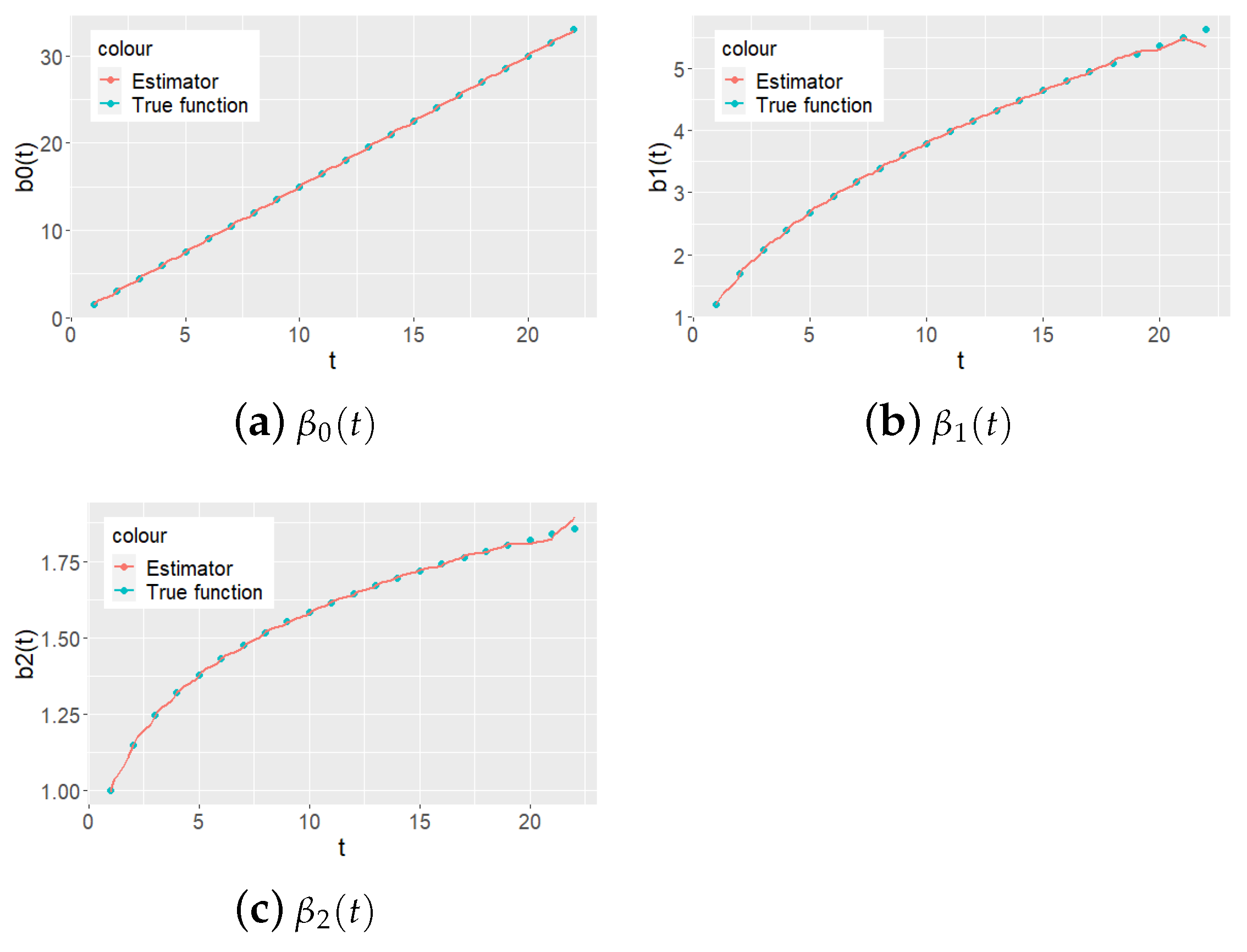
Figure 1 and Figure 2 present the proposed estimated functions of $\mathit{\beta }\left(t\right)$ as a continuous curve and true values of $\mathit{\beta }\left(t\right)$ at time points $t\in \Delta$ as a series of points. Figure 3 and Figure 4 present the estimated functions of $\mathit{\beta }\left(t\right)$ using the local polynomial regression method. In Scenario 1, our method is not significantly superior to polynomial regression. However, in Scenario 2, the term regression method does not fit ${\beta }_2\left(t\right)$ well, and our method estimates ${\widehat{\beta }}_2\left(t\right)$ close to the true value. This is because ${\beta }_2\left(t\right)$ is set up as a trigonometric function rather than a linear combination of power functions. It can be seen that while the local polynomial regression method is suitable for power basis functions, the kernel smoothing method fits the function better, even in such cases.

Figure 1. True values at observed time points and estimated function of $\mathit{\beta }\left(t\right)$ for scenario 1.

Figure 2. True values at observed time points and estimated function of $\mathit{\beta }\left(t\right)$ for scenario 2.

Figure 3. Polynomial regression estimator of $\mathit{\beta }\left(t\right)$ for scenario 1.

Figure 4. Polynomial regression estimator of $\mathit{\beta }\left(t\right)$ for scenario 2.

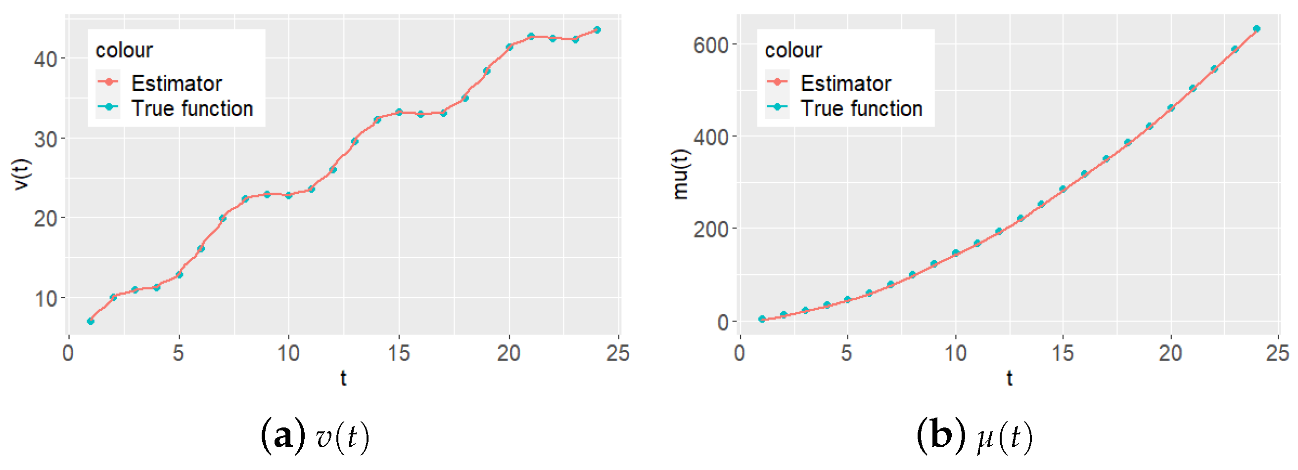
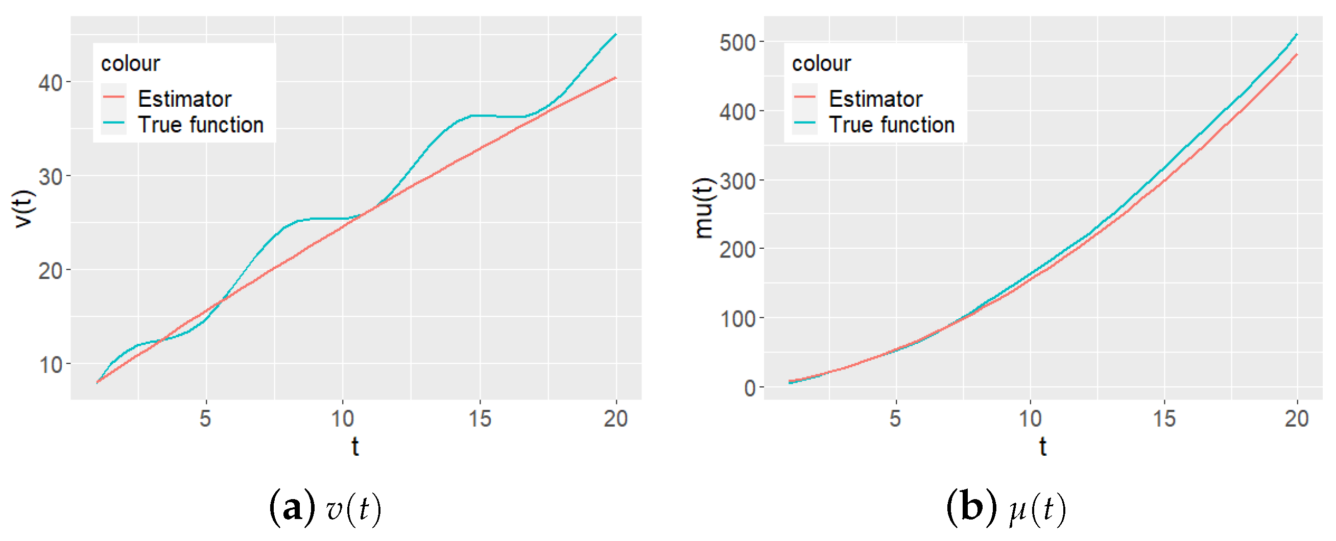
Furthermore, Figure 5 and Figure 6 show the true curves and fitted values of the state function $v\left(t\right)$ and the mean of cumulative mean function $\mu \left(t\right)$. In each figure, the estimated functions approximate to the values of true functions. Figure 7 and Figure 8 show the results of the local polynomial regression method. Similar to the previous conclusion, the method we proposed works better.

Figure 5. True values at observed time points and estimated function of $v\left(t\right)$ and $\mu \left(t\right)$ for scenario 1.

Figure 6. True values at observed time points and estimated function of $v\left(t\right)$ and $\mu \left(t\right)$ for scenario 2.

Figure 7. Polynomial regression estimator of $v\left(t\right)$ and $\mu \left(t\right)$ for scenario 1.

Figure 8. Polynomial regression estimator of $v\left(t\right)$ and $\mu \left(t\right)$ for scenario 2.

4. An Application to MADIT Data

In this section, we validate the proposed estimator with a real data set from a multicenter automatic defibrillator implantation trial (MADIT). MADIT data contain 181 subjects (patients) from 36 centers in the USA that were observed at a total of 134,853 discrete time points. With the 181 patients, 89 of them chose to implant cardiac defibrillators, while another 92 did not. Throughout this section, we encode the ‘implanted’ group as $ICD=1$ and ‘not implanted’ group as $ICD=0$. Since the effect of treatment of whether to implant cardiac defibrillators (ICDs) did not directly induce any medical costs but actually affected the expected survival time, we consider it as the time-independent covariate in the survival sub-model.

The observed patients have six types of costs that can be observed daily from the start to the death time or censoring time: Type 1: hospitalization and emergency department visits; Type 2: outpatient tests and procedures; Type 3: physician/specialist visits; Type 4: community services; Type 5: medical supplies; Type 6: medication. These costs directly drive medical costs, thus they should be considered as time-dependent covariates in the longitudinal process sub-model. It should be pointed out that the whole observation contains quite a lot of data points, so the R-code cannot work for the daily cost data. Therefore, we merge the data by combining 12 days into one time unit.

These data also include the patients’ ID codes, observed survival times in days, and death indicators.

Now, in the data set, we encode the total 181 patients as follows:

• ID code (from 1 to 181);
• Treatment code (1 for ICD and 0 for conventional);
• Observation of survival time;
• Death indicator(1 for death, 0 for censored);
• Merged medical costs of type 1–6.

To analyze this data set, we describe the model as follows:

$$\left\{\begin{array}{c}\begin{array}{cc}\hfill Y_i\left(t\right)=& {\beta }_0\left(t\right)+{\beta }_1\left(t\right)x_{1i}\left(t\right)+{\beta }_2\left(t\right)x_{2i}\left(t\right)+{\beta }_3\left(t\right)x_{3i}\left(t\right)+{\beta }_4\left(t\right)x_{4i}\left(t\right)\hfill \\ \hfill & +{\beta }_5\left(t\right)x_{5i}\left(t\right)+{\beta }_6\left(t\right)x_{6i}\left(t\right)+{ϵ}_i\left(t\right),\hfill \end{array}\hfill \\ h_i\left(t\right)=h_0\left(t\right)exp\{\gamma w_i+\alpha (Y_i\left(t\right)-{ϵ}_i\left(t\right))\},\hfill \end{array}\right.$$

where for $r=1,2,\dots ,6$, $x_{ir}\left(t\right)=1$ if type = 1, otherwise, $x_{ir}\left(t\right)=0$, $w_i=1$ for the ICD group and $w_i=0$ for the not implanted group. The estimated parameters $\widehat{\gamma }$ and $\widehat{\alpha }$ in survival sub-model are obtained by Cox partial maximum likelihood method, they are always asymptotically normal. The estimates of $\gamma$ and $\alpha$ in this paper are attained by calling ‘coxph()’ and ‘method = peicewise-PH-GH’ in the JM package. The Std. Err. and p-value are automatically produced.

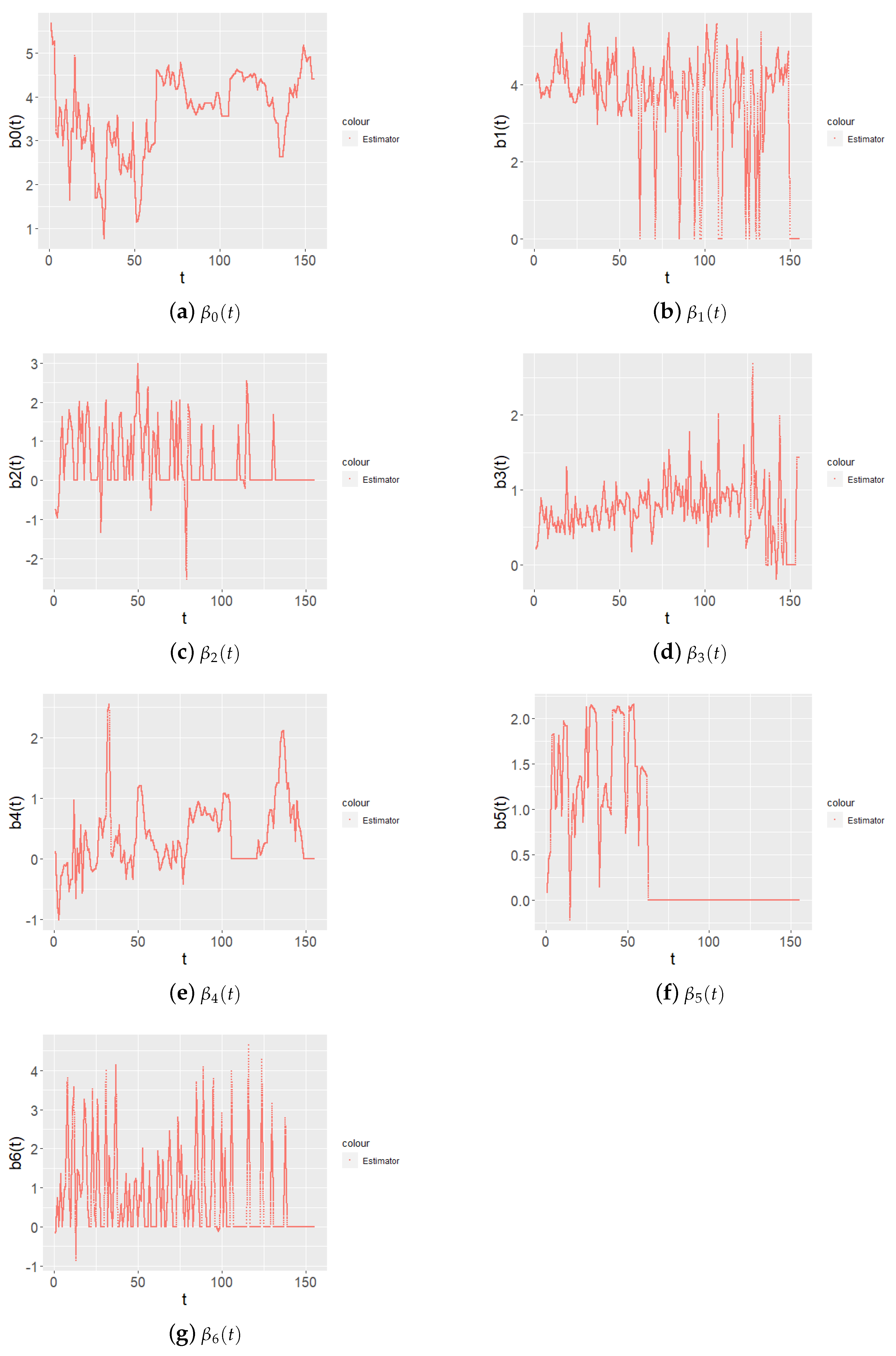
In this case, $\mathit{\beta }\left(t\right)$ can be considered the relationship between the natural logarithm of medical cost and time unit. The fitted curve is illustrated in Figure 9. Time-varying parameters more accurately describe the effect of covariates on state function over time, such as ${\beta }_5\left(t\right)$; after a certain time point, $x_5\left(5\right)$ does not affect the state function, although the in early stage it does.

Figure 9. Estimated function of $\beta \left(t\right)$.

Table 5 shows the estimates of the survival sub-model. The association effect $\alpha$ is positive, which corresponds to reality, that is, patients in a serious life condition require more medical attention. In other words, serious illness leads to higher medical costs, corresponding to lower survival rates. This further supports that our model is efficient and reasonable. However, due to the large p-value of the result, this conclusion is not specific, which should be further tested using a large sample in future research. The treatment effect $\gamma$ is negative, which corresponds to reality, that is, an automatic defibrillator implantation trial can reduce the risk of death. In other words, the ‘implanted’ group (ICD = 1) has a lower risk of death. This conclusion is supported by the small p-value of the result.

Table 5. Estimate results of the event process.

Parameter	Value	Std. Err.	p-Value
Treatment	−1.2219	0.3362	0.0003
Association effect	0.2519	0.2087	0.2274

Table 6 presents the estimated values of the cumulative cost for 5 years and the total treatment period. Comparing Sub-figure(a) with Sub-figure(b) in Figure 10 and Figure 11, we realize that the fitted points for the mean medical cost based on the current approach better describe the elaborate trajectories of medical costs, and the result for the fitted points of the cumulative mean medical cost based on the current approach exhibit a similar trend to Li’s [19] result; however, the result is more accurate and shows continuous change, which, in turn, leads to improved understanding of real-world data.

Table 6. Estimated cumulative costs for 5 years and total period.

Year 1	Year 2	Year 3	Year 4	Year 5	Total
21,661.83	45,403.10	67,981.31	101,983.30	134,749.20	135,412.00

Figure 10. Fitted points of cost based on current approach and the semi-parametric estimating approach.

Figure 11. Fitted points of cumulative cost based on current approach and the semi-parametric estimating approach.

Compared with parametric/semi-parametric estimation, our method suggests a smoother time-varying mean medical cost function, which is no longer a straight line with an observable change rate, but exhibits more fluctuations over time. In practical situations, government agencies or insurance companies would not know which treatment was selected by a patient. The estimated cumulative mean function provides them with a more accurate statistical decision recommendation for macro allocation. For example, we should consider the additional changes in medical costs because they would suddenly increase or decrease at distinct time points.

Moreover, the estimated marginal survival function is smoother compared with the Kaplan–Meier estimator. The result is similar to research by Li’s [19], as shown in Figure 12. The solid line is the estimated survival rate, and the dotted line represents the $95\%$ confidence interval of the estimated survival rate.

Figure 12. Marginal survival compared with Kaplan–Meier estimator.

5. Discussion

Generally, some estimate methods can lead to biased estimates in the model, and the time-varying coefficient model compensates for this shortcoming. In this study, we provide an estimation of the time-varying coefficient using the kernel function technique. When the covariates are continuous, the continuous state function can be obtained, allowing for the derivation of the continuous cumulative mean state function. In summary, our method is more precise because the kernel function smooths the estimator; more importantly, the proposed estimator at the original observed true points is unbiased. Theorem 2 demonstrates this perspective. In our numerical simulation and application analysis, we consider the observation interval to be a unit of 1, and we chose a bandwidth h of 1 in the kernel smoothing function. Notably, in cases where the observation time interval is not 1 or involves interval censoring, we must choose the appropriate bandwidth. Many studies on kernel function have proposed methods for choosing the bandwidth. In general, too large a bandwidth distorts data, and too small a bandwidth does not lead to a smooth continuous function. Moreover, as $h\to \infty$, $\mathit{\beta }\left(t\right)$ turns out to be a series of constants, that is, a time-independent parametric estimator.

In this study, we do not consider the random effect coefficients in the longitudinal data model, and the correlation that may exist among repeated observations within individuals is ignored. If we consider the random effect coefficients, we will not obtain Theorem 2, but we can still obtain Theorem 3. In future studies, random effects should be considered in longitudinal models, which may yield better results.

Furthermore, the estimation of the time-varying coefficient using the kernel function technique can be extended to multiple longitudinal outcomes, and the justification for the survival sub-model would need a multi-dimensional association coefficient. The methods proposed in [20] may be applicable.