Combination Test for Mean Shift and Variance Change

Abstract

This paper considers a new mean-variance model with strong mixing errors and describes a combination test for the mean shift and variance change. Under some stationarity and symmetry conditions, the important limiting distribution for a combination test is obtained, which can derive the limiting distributions for the mean change test and variance change test. As an application, an algorithm for a three-step method to detect the change-points is given. For example, the first step is to test whether there is at least a change-point. The second and third steps are to detect the mean change-point and the variance change-point, respectively. To illustrate our results, some simulations and real-world data analysis are discussed. The analysis shows that our tests not only have high powers, but can also determine the mean change-point or variance change-point. Compared to the existing methods of cpt.meanvar and mosum from the R package, the new method has the advantages of recognition capability and accuracy.

1. Introduction

In the paper [1], statistical methods of control for manufacturing processes were first proposed. However, the issue of change-points initially appeared in the context of quality control, where staff typically observe the output of a production line, aiming to detect signals deviating from acceptable levels while observing the data. Since the seminal paper [2], the cumulative sum (CUSUM) test has been one of the most popular methods for detecting a parameter change in statistical models. CUSUM tests of the mean change-point and the variance change-point have played a central role in detecting abnormal signals during quality control and changes in financial time series and other fields. For example, the authors of the papers [3,4] considered CUSUM tests for the mean change-point model with independent errors and linear processes, respectively; the papers [5,6] investigated CUSUM tests for the variance change-point model with independent normal errors and independent errors, respectively. For further studies, reference can be made to [7,8,9,10] and the sources detailed therein. Combining the change-point of mean with change-point of variance, this paper considers a change-point model with mean shift and variance change. For $T\ge 2$, we consider a time series $\left\{X_t\right\}$ to be a mean-variance model as

$$X_t={\mu }_t+{\sigma }_t{e}_t,1\le t\le T,$$

(1)

where $-\infty <{\mu }_t<\infty$ and ${\sigma }_t>0$ are the mean and variance parameters, respectively. Since the condition of strong mixing ($\alpha$-mixing) is more general in time series [11], we consider the error sequence $\left\{e_t\right\}$ to be a $\alpha$-mixing sequence with a mean of zero and variance of one. Let us recall the definition of $\alpha$-mixing. Let $N=\{1,2,\cdots \}$ and denote ${\mathcal{F}}_k^T=\sigma (e_t,k\le t\le T,t\in N)$ to be the $\sigma$-fields generated by random variables $e_k,e_{k+1},\cdots ,e_T$, $1\le k\le T$. For $t\ge 1$, we define

$$\alpha \left(t\right)=\underset{m\in N}{sup}\underset{A\in {\mathcal{F}}_1^m,B\in {\mathcal{F}}_{m+t}^{\infty }}{sup}|\mathrm{P}(A\cap B)-\mathrm{P}\left(A\right)\mathrm{P}\left(B\right)|.$$

Definition 1.

If $\alpha \left(t\right)\to 0$ as $t\to \infty$, then $\{e_t,t\ge 1\}$ is called a strong mixing or α-mixing sequence.

In the mean-variance model (1), we monitor the mean change-point with the CUSUM statistic

$$U_{k,1}=(\frac{k(T-k)}{T})[\frac{1}{k}\sum _{t=1}^k{X}_t-\frac{1}{T-k}\sum _{t=k+1}^T{X}_t],1\le k\le T-1,$$

(2)

and monitor the variance change-point with the CUSUM statistic

$$U_{k,2}=(\frac{k(T-k)}{T})[\frac{1}{k}\sum _{t=1}^k{(X_t-\overline{X})}^2-\frac{1}{T-k}\sum _{t=k+1}^T{(X_t-\overline{X})}^2],1\le k\le T-1,$$

(3)

where $\overline{X}=\frac{1}{T}{\sum }_{t=1}^T{X}_t$.

To improve the power of the statistics of the mean change-point and the variance change-point, we use the combination statistic

$$\begin{array}{c}\hfill g(T,k):={(g_1(T,k),g_2(T,k))}^{\top }:={(\frac{1}{\sqrt{T}}{U}_{k,1},\frac{1}{\sqrt{T}}{U}_{k,2})}^{\top },\end{array}$$

(4)

where $U_{k,1}$ and $U_{k,2}$ are defined by (2) and (3), respectively. Here, ⊤ represents the transpose of the vector. Under the assumption of no change in the mean or variance, for all $T\ge 2$, the model (1) can be summarized in the null hypothesis $H_0$ as

$${\mu }_1={\mu }_2=\cdots ={\mu }_T={\mu }_0\mathrm{and}{\sigma }_1={\sigma }_2\cdots ={\sigma }_T={\sigma }_0,$$

(5)

where $-\infty <{\mu }_0<\infty$ and $0<{\sigma }_0<\infty$. The change-point alternative hypothesis $H_A$ is that there is an integer $k_1^{\ast }$ such that ${\mu }_1=\cdots ={\mu }_{k_1^{\ast }}\ne {\mu }_{k_1^{\ast }+1}=\cdots ={\mu }_T$ or there is an integer $k_2^{\ast }$ such that ${\sigma }_1=\cdots ={\sigma }_{k_2^{\ast }}\ne {\sigma }_{k_2^{\ast }+1}=\cdots ={\sigma }_T$.

In this paper, we consider the mean-variance model (1) with $\alpha$-mixing errors and investigate the limiting distributions for the statistics related to $g(T,k)$ under the null hypothesis $H_0$ by (5). For example, if $\underset{1\le k\le T-1}{max}g{(T,k)}^{T}g(T,k)$ is smaller than a critical value (see details in Remark 2), then there is no evidence of a mean change or variance change in the mean-variance model (1). Otherwise, if $\underset{1\le k\le T-1}{max}\left|g_1(T,k)\right|$ is larger than another critical value (see details in Remark 2), the mean change-point location is suggested by

$${\widehat{k}}_{T,1}=\underset{1\le k\le T-1}{argmax}|g_1(T,k)|=\underset{1\le k\le T-1}{argmax}\left|U_{k,1}\right|.$$

(6)

If $\underset{1\le k\le T-1}{max}\left|g_2(T,k)\right|$ is larger than this critical value, the variance change-point location is suggested by

$${\widehat{k}}_{T,2}=\underset{1\le k\le T-1}{argmax}|g_2(T,k)|=\underset{1\le k\le T-1}{argmax}\left|U_{k,2}\right|.$$

(7)

Compared with existing methods for determining change-points, such as cpt.meanvar from the R package changepoint in [12] and mosum from the R package mosum in [13], we will show that our tests not only have high powers, but also determine the change-points as the mean change-point or variance change-point. Further details are provided in Section 3, Section 4 and Section 5.

In addition to the change-point studies referred to above, many scholars have sought to extend the change-points of the mean and variance for both independent and dependent data. For the mean change-point example, in [14,15,16], CUSUM estimators were investigated with dependent errors; in [17], a weighted CUSUM estimator was studied using an infinite variance $AR\left(p\right)$ process; in [18,19], a self-normalization method was used to test the mean change-point in a time series; in [20,21], data-driven methods were used to investigate the mean shift and variance change; in [22,23,24], CUSUM estimators were discussed regarding the mean change-point with panel data. For the variance change-point example, the Schwarz information criterion (SIC) estimator of variance change was studied with independent normal errors in [25]; ref. [26] extended the CUSUM estimator in [5] with normal data to infinite moving average processes; in [27], a weighted variances test was considered based on independent errors; covariance structure change was studied with linear processes in [28]. In addition, the authors of [29] considered a CUSUM test of parameter changes in a time series model; refs. [30,31] reported changes in a variance inflation factor (VIF) regression model and a linear regression model; the authors of ref. [32] considered changes in parameters using the Shiryaev–Roberts statistics; in ref. [33], the change of covariance structure in multivariate time series were considered; refs. [34,35,36] considered multiple change-points; in ref. [37], the authors investigated a Bayesian method for the change-point; the authors of ref. [38] investigated a new class of weighted CUSUM estimators of the mean change-point; in ref. [39], the least sum of the squared error (LSSE) and maximum log-likelihood (MLL) methods in the estimation of the change-point were examined; in ref. [40], multivariate change-points in a mean vector and/or covariance structure were considered; and ref. [41] discussed a CUSUM estimator in an ARMA–GARCH model. Furthermore, a test for the detection of outliers for continuous distribution data was investigated in [42]; refs. [43,44], respectively, investigated change-point problems with a nonstationary time series and the volatility of conditional heteroscedasticity, respectively.

It is pointed out that the $\alpha$-mixing sequence is very general in time series. For example, consider an infinite order moving average (MA(∞)) process $X_t={\sum }_{i=0}^{\infty }{a}_i{e}_{t-i},t\ge 1$, where $a_i\to 0$ exponentially fast, and $\left\{e_t\right\}$ is an $i.i.d.$ sequence. If the probability density function of $e_t$ exists (such as normal, Cauchy, exponential, and uniform distributions), then $\left\{X_t\right\}$ is an $\alpha$-mixing with exponentially decaying coefficients. The strictly stationary time series, including the autoregressive moving average (ARMA) processes and geometrically ergodic Markov chains, are the $\alpha$-mixing processes. For further studies of $\alpha$-mixing, reference can be made to [45,46] for limit theorems, refs. [47,48] for central limit theorem, refs. [49,50,51,52] for regression models, etc.

The rest of this paper is organized as follows. Some assumptions are provided in Section 2. By some stationarity and symmetry conditions, the limit distribution for the combination statistic $g(T,k)$ will be shown under the null hypothesis (5) in Section 2, which can derive the limiting distributions of the CUSUM statistics $g_1(T,k)$ for the mean change and $g_2(T,k)$ for the variance change, respectively. As an application, we give a three-step algorithm to detect the change-points in Section 3. For example, in the first step, we do the combination test to check whether there is at least a change-point or not; in the second step, we do the mean test to detect the mean change-point; in the third step, we use the variance test to detect the variance change-point. In Section 4 of simulation, it will show that our method has a better performance than the methods of as cpt.meanvar [12] and mosum [13]. We also use three examples of real-world data to detect the mean change-point and variance change-point in Section 5. In addition, some conclusions and future work will be discussed in Section 6. Last, the proofs of the main results are presented in Section 7.

Throughout the paper, as $T\to \infty$, let $\stackrel{P}{\to }$ and $\stackrel{d}{\to }$ denote the convergence in probability and distribution, respectively. Let $C,C_1,C_2,C_3,\cdots$ denote some positive constants not depending on T, which may be different in various places. If X and Y have the same distribution, we denote it as $X\sim Y$. In addition, second-order stationarity means that $(e_1,e_{1+k})\sim (e_t,e_{t+k})$ for all $t\ge 1$ and $k\ge 1$.

2. Main Results

First, we list some assumptions as follows:

Assumption 1.

Consider the model (1), where $\{e_t,t\ge 1\}$ is a stationarity sequence of α-mixing random variables with $\mathrm{E}{e}_t=0$, $\mathrm{E}{e}_t^2=1$ for all $t\ge 1$. In addition, for some $\delta >0$, let $\underset{t\ge 1}{sup}\mathrm{E}{\left|e_t\right|}^{4+2\delta }<\infty$ and ${\sum }_{t=1}^{\infty }{\alpha }^{\frac{\delta }{2+\delta }}\left(t\right)<\infty$.

Assumption 2.

Let ${\mu }_0$ be defined in (5) and

$$\begin{array}{c}\hfill \underset{T\to \infty }{lim}\frac{1}{T}\mathrm{Var}({\displaystyle {\displaystyle \sum }_{t=1}^T}{X}_t)=s_1^2>0,\underset{T\to \infty }{lim}\frac{1}{T}\mathrm{Var}({\displaystyle {\displaystyle \sum }_{t=1}^T}{(X_t-{\mu }_0)}^2)=s_2^2>0,\end{array}$$

(8)

$$\begin{array}{c}\hfill \underset{T\to \infty }{lim}\frac{1}{T}{\displaystyle {\displaystyle \sum }_{i=1}^T}{\displaystyle {\displaystyle \sum }_{j=1}^T}\mathrm{Cov}[(X_i-{\mu }_0),{(X_j-{\mu }_0)}^2]=0.\end{array}$$

(9)

Assumption 3.

Let $\{e_t,t\ge 1\}$ be a second-order stationarity sequence of α-mixing random variables with $\mathrm{E}{e}_1=0$ and $\mathrm{E}{e}_1^2=1$. For some $\delta >0$, assume that $\mathrm{E}|e_1{|}^{8+4\delta }<\infty$ and ${\sum }_{t=1}^{\infty }{\alpha }^{\frac{\delta }{2+\delta }}\left(t\right)<\infty$. In addition, let $\mathrm{E}{e}_1{e}_{1+j}^2=0$ for all $j\ge 0$.

Assumption 4.

Let

$$s_1^2:={\gamma }_1\left(0\right)+2\sum _{h=1}^{\infty }{\gamma }_1\left(h\right)>0,s_2^2:={\gamma }_2\left(0\right)+2\sum _{h=1}^{\infty }{\gamma }_2\left(h\right)>0,$$

(10)

where ${\gamma }_1\left(h\right)=\mathrm{Cov}(X_1,X_{1+h})=\mathrm{Cov}((X_1-{\mu }_0),(X_{1+h}-{\mu }_0))$ and ${\gamma }_2\left(h\right)=\mathrm{Cov}({(X_1-{\mu }_0)}^2,{(X_{1+h}-{\mu }_0)}^2)$ for $h=0,1,2,\cdots$.

Assumption 5.

Let $\{h_T,T\ge 1\}$ be a sequence of positive integers satisfying

$$h_T\to \infty asT\to \infty and{h}_T=O\left(T^{\beta }\right)forsome\beta \in (0,1/2).$$

(11)

Remark 1.

The moment conditions and mixing coefficients of α-mixing sequence $\left\{e_t\right\}$ in Assumption 1 are used by many researchers, see [46,51], etc. The conditions (8) in Assumption 2 are the limiting variances for partial sums of $\{\frac{X_t-{\mu }_0}{\sqrt{T}}\}$ and $\{\frac{{(X_t-{\mu }_0)}^2}{\sqrt{T}}\}$. The condition (9) in Assumption 2 is a symmetry condition, which requires the limiting for partial sums of covariance of $\{\frac{X_t-{\mu }_0}{\sqrt{T}}\}$ and $\{\frac{{(X_t-{\mu }_0)}^2}{\sqrt{T}}\}$ to be zero. For example, let $f(x,y;k)$ denote the joint probability density function of random variables $X_t-{\mu }_0$ and $X_{t+k}-{\mu }_0$ for all $t\ge 1$ and $k\ge 1$. Let $f(x,y;k)$ be symmetrical, i.e., $f(x,y;k)=f(-x,-y;k)$ for all $x,y\in R$. It is easy to check that $\mathrm{E}\left[(X_t-{\mu }_0){(X_{t+k}-{\mu }_0)}^2\right]=-\mathrm{E}\left[(X_t-{\mu }_0){(X_{t+k}-{\mu }_0)}^2\right]$, which implies $\mathrm{E}\left[(X_t-{\mu }_0){(X_{t+k}-{\mu }_0)}^2\right]=0$ for all $t\ge 1$ and $k\ge 1$. In addition, it has $\mathrm{E}(X_t-{\mu }_0)=0$ and $\mathrm{E}{(X_t-{\mu }_0)}^3=0$ for all $t\ge 1$. Obviously, the binary normal distribution can satisfy the conditions for this example. Thus, the condition of (9) is satisfied. The second-order stationarity condition in Assumption 3 is provided to obtain $s_1^2$ and $s_2^2$ in Assumption 2. They are the long-run variances $s_1^2$ and $s_2^2$ in (10). To estimate these long-run variances $s_1^2$ and $s_2^2$, we use Assumption 4 and the sample autocovariance functions to give their estimators ${\widehat{s}}_{T,1}^2$ and ${\widehat{s}}_{T,2}^2$ in (16). A similar condition (11) can be seen in [26].

Second, we study the limiting distribution of combination statistic $g(T,k)$ in (4) under the null hypothesis $H_0$ by (5). We denote $\lfloor x\rfloor$ as the greatest integer not exceeding x. Throughout the paper, let $\{W_1^0\left(x\right),x\in [0,1]\}$ and $\{W_2^0\left(x\right),x\in [0,1]\}$ be two independent standard Brownian bridges, ⇒ denote the convergence in distribution in the Skorokhod space $D[0,1]$.

Theorem 1.

In model (1), let the Assumptions 1 and 2 be satisfied. Then, under the null hypothesis $H_0$ defined by (5), for $0<k=\lfloor xT\rfloor <T$ and $x\in [0,1]$, it has

$$\begin{array}{c}\hfill g{(T,k)}^{\top }g(T,k)\Rightarrow \sum _{i=1}^2{s}_i^2{\left(W_i^0\left(x\right)\right)}^2,asT\to \infty ,\end{array}$$

(12)

where $g(T,k)$, $s_1^2$ and $s_2^2$ are defined by (4) and (8), respectively. Combining with the continuous mapping theorem, we obtain

$$\begin{array}{c}\hfill \underset{1\le k\le T-1}{max}g{(T,k)}^{\top }g(T,k)\stackrel{d}{⟶}\underset{0\le x\le 1}{sup}\sum _{i=1}^2{s}_i^2{\left(W_i^0\left(x\right)\right)}^2,asT\to \infty .\end{array}$$

(13)

Usually, the $s_1^2$ and $s_2^2$ in (8) are unknown. We should estimate them. By the second stationarity in Assumption 3, it is easy to obtain the long-run variances $s_1^2$ and $s_2^2$ defined by (10). In the next, we discuss the estimators of $s_1^2$ and $s_2^2$. Let $Z_t=X_t-\overline{X}$, $1\le t\le T$. Then, ${\gamma }_1\left(h\right)$ and ${\gamma }_2\left(h\right)$ defined in (10) can be, respectively, estimated by ${\widehat{\gamma }}_1\left(h\right)$ and ${\widehat{\gamma }}_2\left(h\right)$ as

$${\widehat{\gamma }}_1\left(h\right)=\frac{1}{T}\sum _{t=1}^{T-h}{Z}_t{Z}_{t+h},0\le h<T,$$

(14)

and

$${\widehat{\gamma }}_2\left(h\right)=\frac{1}{T}\sum _{t=1}^{T-h}(Z_t^2-\overline{Z^2})(Z_{t+h}^2-\overline{Z^2}),0\le h<T,$$

(15)

where $\overline{Z^2}=\frac{1}{T}{\sum }_{t=1}^T{Z}_t^2$ and $\overline{X}=\frac{1}{T}{\sum }_{t=1}^T{X}_t$.

Thus, the estimators of $s_1^2$ and $s_2^2$ are, respectively, suggested by

$${\widehat{s}}_{T,1}^2:={\widehat{\gamma }}_1\left(0\right)+2\sum _{h=1}^{h_T}{\widehat{\gamma }}_1\left(h\right),{\widehat{s}}_{T,2}^2:={\widehat{\gamma }}_2\left(0\right)+2\sum _{h=1}^{h_T}{\widehat{\gamma }}_2\left(h\right),$$

(16)

where ${\widehat{\gamma }}_1\left(h\right)$ and ${\widehat{\gamma }}_2\left(h\right)$ are defined by (14) and (15).

Lemma 1.

In model (1), let the Assumptions 3–5 be satisfied. Under the null hypothesis $H_0$ defined by (5), we obtain

$${\widehat{s}}_{T,1}^2\stackrel{P}{⟶}{s}_1^2,{\widehat{s}}_{T,2}^2\stackrel{P}{⟶}{s}_2^2,$$

(17)

where $s_1^2$, $s_2^2$, ${\widehat{s}}_{T,1}^2$ and ${\widehat{s}}_{T,2}^2$ are defined by (10) and (16), respectively.

For $1\le k\le T-1$, denote the combination statistic

$$\begin{array}{c}\hfill f(T,k):={(\frac{1}{\sqrt{{\widehat{s}}_{T,1}^2}}{g}_1(T,k),\frac{1}{\sqrt{{\widehat{s}}_{T,2}^2}}{g}_2(T,k))}^{\top }={(\frac{1}{\sqrt{T{\widehat{s}}_{T,1}^2}}{U}_{k,1},\frac{1}{\sqrt{T{\widehat{s}}_{T,2}^2}}{U}_{k,2})}^{\top },\end{array}$$

(18)

where $U_{k,1}$, $U_{k,2}$, $g_1(T,k)$, $g_2(T,k)$, ${\widehat{s}}_{T,1}^2$ and ${\widehat{s}}_{T,2}^2$ are defined by (2)–(4) and (16), respectively.

Combining Theorem 1 with Lemma 1, we obtain two corollaries as follows:

Corollary 1.

In model (1), let the Assumptions 3–5 be fulfilled. Under the null hypothesis $H_0$ defined by (5), for $0<k=\lfloor xT\rfloor <T$ and $x\in [0,1]$, we have

$$\begin{array}{c}\hfill f{(T,k)}^{\top }f(T,k)\Rightarrow \sum _{i=1}^2{\left(W_i^0\left(x\right)\right)}^2,asT\to \infty ,\end{array}$$

(19)

where $W_1^0\left(x\right)$ and $W_2^0\left(x\right)$ are defined in (12). Thus,

$$\begin{array}{c}\hfill \underset{1\le k\le T-1}{max}f{(T,k)}^{\top }f(T,k)\stackrel{d}{⟶}\underset{0\le x\le 1}{sup}\sum _{i=1}^2{\left(W_i^0\left(x\right)\right)}^2,asT\to \infty .\end{array}$$

(20)

Corollary 2.

In model (1), let the Assumptions 3–5 be fulfilled. Under the null hypothesis $H_0$ defined by (5), it has

$$\underset{1\le k\le T-1}{max}|\frac{g_1(T,k)}{\sqrt{{\widehat{s}}_{T,1}^2}}|\stackrel{d}{⟶}\underset{0\le x\le 1}{sup}|W_1^0\left(x\right)|,\underset{1\le k\le T-1}{max}|\frac{g_2(T,k)}{\sqrt{{\widehat{s}}_{T,2}^2}}|\stackrel{d}{⟶}\underset{0\le x\le 1}{sup}\left|W_2^0\left(x\right)\right|,$$

(21)

where $\frac{g_1(T,k)}{\sqrt{{\widehat{s}}_{T,1}^2}}$ and $\frac{g_2(T,k)}{\sqrt{{\widehat{s}}_{T,2}^2}}$ are defined by (18), $W_1^0\left(x\right)$ and $W_2^0\left(x\right)$ are defined in (12).

Remark 2.

For $i=1,2$, by (11.38) in [53], it is presented that

$$P(\underset{x\in [0,1]}{sup}|W_i^0\left(x\right)|\le y)=1+2\sum _{k=1}^{\infty }{(-1)}^{k}exp(-2k^2{y}^2),y>0,$$

(22)

where $W_1^0\left(x\right)$ and $W_2^0\left(x\right)$ be defined in (12). Let α ($0<\alpha <1$) be the level of significance. For $l\ge 1$, let $W_1^0\left(x\right),\cdots ,W_l^0\left(x\right)$ be independent standard Brownian bridges for $x\in [0,1]$. Then the distribution of

$$\underset{0\le x\le 1}{sup}\sum _{i=1}^l{\left(W_i^0\left(x\right)\right)}^2$$

(23)

was derived by Kiefer [54], which has a series Fourier-Bessel expansions. It is not easy to calculate the critical values for this distribution. Lee et al. [29] considered the problem of testing for parameter changes in time series models based on the CUSUM statistics and obtained the limiting distribution (23). They used the Monte Carlo method to obtain the critical values $c_{\alpha }$ with different α and l. For example, when $l=2$, the critical values $c_{\alpha }$ are calculated as $c_{0.05}=2.408$ and $c_{0.1}=2.054$ (see [29]).

If $\underset{1\le k\le T-1}{max}f{(T,k)}^{\top }f(T,k)\le c_{\alpha }$, there is no evidence of a mean change or variance change. Otherwise, we conclude that there is at least a mean change-point or a variance change-point.

Similar to the multiple testing problems, by (22), we take the critical value $d_{\alpha /2}$ for the distribution of $\underset{0\le x\le 1}{sup}\left|W_1^0\left(x\right)\right|$ to do the tests of the mean change-point and variance change-point, in order to control the type I error. For example, $d_{0.025}=1.48$, $d_{0.05}=1.358$. If $\underset{1\le k\le T-1}{max}|\frac{g_1(T,k)}{\sqrt{{\widehat{s}}_{T,1}^2}}|\le d_{\alpha /2}$, there is no evidence of a mean change. Otherwise, we conclude that there is a mean change-point, and its time location $k_1^{\ast }$ is defined in (6).

Meanwhile, by (22), the p-value of $\underset{1\le k\le T-1}{max}|\frac{g_1(T,k)}{\sqrt{{\widehat{s}}_{T,1}^2}}|$ can be defined by $p_{v1}$ as

$$p_{v1}=\mathrm{P}(\underset{x\in [0,1]}{sup}|W_1^0\left(x\right)|>y_0)=-2\sum _{k=1}^{\infty }{(-1)}^{k}exp(-2k^2{y}_0^2),$$

(24)

where $y_0=\underset{1\le k\le T-1}{max}|\frac{g_1(T,k)}{\sqrt{{\widehat{s}}_{T,1}^2}}|$. Similarly, let $d_{\alpha /2}$ be the critical value for the distribution of $\underset{0\le x\le 1}{sup}|W_2^0\left(x\right)|$. If $\underset{1\le k\le T-1}{max}|\frac{g_2(T,k)}{\sqrt{{\widehat{s}}_{T,2}^2}}|\le d_{\alpha /2}$, there is no evidence of a variance change. Otherwise, we conclude that there is a variance change-point, and its time location $k_2^{\ast }$ is suggested in (7).

In addition, the p-value $p_{v2}$ of $\underset{1\le k\le T-1}{max}|\frac{g_2(T,k)}{\sqrt{{\widehat{s}}_{T,2}^2}}|$ can be defined by (24), where $|W_1^0\left(x\right)|$ is replaced by $|W_2^0\left(x\right)|$ and $y_0$ is $\underset{1\le k\le T-1}{max}|\frac{g_2(T,k)}{\sqrt{{\widehat{s}}_{T,2}^2}}|$.

3. The Three-Step Algorithm

Based on the combination statistic $f(T,k)$ in Corollary 1, the mean change statistic $g_1(T,k)$ and variance change statistic $g_2(T,k)$ in Corollary 2, we give a three-step algorithm to test the changes in mean and variance in Algorithm 1, i.e., the combination test, mean change test, and variance change test. In the following algorithm, we assume that there is at most one mean and one variance in the time series. If there are more change-points, we will give the discussion in Remark 3 to detect them.

Remark 3.

It can be seen that the CUSUM statistic $U_{k,2}$ of variance change in (3) contains the sample mean statistic, while the CUSUM statistic $U_{k,1}$ of mean change in (2) does not contain the sample variance statistic. One can use $U_{k,2}^{\ast }$

$$U_{k,2}^{\ast }=(\frac{k(T-k)}{T})[\frac{1}{k}\sum _{t=1}^k{(X_t-{\overline{X}}_k)}^2-\frac{1}{T-k}\sum _{t=k+1}^T{(X_t-{\overline{X}}_{T-k})}^2],1\le k\le T-1,$$

to replace $U_{k,2}$, where ${\overline{X}}_k=\frac{1}{k}{\sum }_{t=1}^k{X}_t$ and ${\overline{X}}_{T-k}=\frac{1}{T-k}{\sum }_{t=k+1}^T{X}_t$. However, the proofs of limiting distribution and consistency estimator based on $U_{k,2}^{\ast }$ will be complicated. Thus, we consider $U_{k,2}$ to construct the variance change-point estimator. That is why we do the mean change test in Step 2 before the test of variance change in this paper. To reduce the impact of mean change on the variance change test, we can construct the modified data $X_1^{\ast },X_2^{\ast },\cdots ,X_T^{\ast }$ if we find a mean change-point. Then, we go to do Step 3 of the variance change test. Since it is assumed that there is at most one mean and one variance in the time series, Algorithm 1 is terminated after Step 3. If there are more change-points, we can modify the process $\left\{X_t^{\ast \ast }\right\}$ by the variance change. For example, base on the data $\{X_1,X_2,\cdots ,X_T\}$ (or the modified data $\{X_1^{\ast },X_2^{\ast },\cdots ,X_T^{\ast }$}), let the modified process $X_t^{\ast \ast }$ as

$$X_t^{\ast \ast }=\{\begin{array}{cc}{X}_t,\hfill & t\le {\widehat{k}}_{T,2},\hfill \\ {\lambda }_T^{-1/2}{X}_t,\hfill & t>{\widehat{k}}_{T,2},\hfill \end{array}$$

where ${\lambda }_T={\widehat{\sigma }}_{T,2}^2/{\widehat{\sigma }}_{T,1}^2$, ${\widehat{\sigma }}_{T,1}^2=\frac{1}{{\widehat{k}}_{T,2}}{\sum }_{t=1}^{{\widehat{k}}_{T,2}}{(X_t-\overline{X})}^2$, ${\widehat{\sigma }}_{T,2}^2=\frac{1}{T-{\widehat{k}}_{T,2}}{\sum }_{t=1+{\widehat{k}}_{T,2}}^T{(X_t-\overline{X})}^2$ and $\overline{X}=\frac{1}{T}{\sum }_{t=1}^T{X}_t$. Then, based on the modified data $\{X_1^{\ast \ast },\cdots ,X_T^{\ast \ast }\}$, we can combine the three-step algorithm with iterative methods to detect more change-points. For further details, one can refer to [20,21] and the sources detailed therein.

For further studies of multiple change-point detection, reference can be made to [35] and the sources detailed therein. Next, we should discuss the measure of accuracy for the multiple change-point detection. Based on a time series observation of $\{X_1,X_2,\cdots ,X_T\}$, assume that there are $L_0$ change-points denoted by $k_1^{\ast },k_2^{\ast },\cdots ,k_{L_0}^{\ast }$. By the change-point detection methods, it is assumed to detect ${\widehat{L}}_T$ change-points denoted by ${\widehat{k}}_{T,1},{\widehat{k}}_{T,2},\cdots ,{\widehat{k}}_{T,{\widehat{L}}_T}$. Following [55,56], a set of correctly detected change-points is defined as True Positive (TP):

$$TP=\{k_i^{\ast }|\exists {\widehat{k}}_{T,j}:|{\widehat{k}}_{T,j}-k_i^{\ast }|\le m\},i=1,2,\dots ,L_{0}and0\le j\le {\widehat{L}}_T,$$

(25)

where m is a margin size with $m>0$. Then, the Precision, Recall, and F1-score are defined as follows

$$\mathrm{Precision}=\frac{\left|TP\right|}{L_0},\mathrm{Recall}=\frac{\left|TP\right|}{{\widehat{L}}_T},\mathrm{F}1\text{-}\mathrm{score}=2\frac{\mathrm{Precision}\times \mathrm{Recall}}{\mathrm{Precision}+\mathrm{Recall}},$$

(26)

where $\left|TP\right|$ denotes the number of set $TP$.

Algorithm 1 Three-step algorithm

Input: Data: $\{X_1,X_2,\cdots ,X_T\}$, set the level of significance $\alpha$, the critical values $c_{\alpha }$ and $d_{\alpha /2}$ defined in Remark 2. Denote $\mathcal{K}$ the estimator of change-point location.    Initialize:$\mathcal{K}\leftarrow \varnothing$  /* Step 1: Do the combination test */    if$\underset{1\le k\le T-1}{max}f{(T,k)}^{\top }f(T,k)$ in (20) is less than $c_{\alpha }$ then       There is no evidence of a mean change or variance change, and the algorithm is terminated.    else    There is at least a mean change-point or variance change-point, and Step 2 is started.   /* Step 2: Do the mean change test */       if $\underset{1\le k\le T-1}{max}|\frac{g_1(T,k)}{\sqrt{{\widehat{s}}_{T,1}^2}}|$ in (21) is less than $d_{\alpha /2}$ then         There is no evidence of a mean change, and Step 3 is started.       else      There is a mean change-point suggested by ${\widehat{k}}_{T,1}$ in (6). Denote $({\widehat{k}}_{T,1},1)$, where 1 stands the change in mean. Do $\mathcal{K}\leftarrow ({\widehat{k}}_{T,1},1)$. In addition, take the modified the process $X_t^{\ast }$ by the mean change as $$X_t^{\ast }=\{\begin{array}{ll}{X}_t,& t\le {\widehat{k}}_{T,1},\\ X_t-({\overline{\theta }}_{T,2}-{\overline{\theta }}_{T,1}),& t>{\widehat{k}}_{T,1},\end{array}$$      where ${\overline{\theta }}_{T,1}=\frac{1}{{\widehat{k}}_{T,1}}{\sum }_{t=1}^{{\widehat{k}}_{T,1}}{X}_t$ and ${\overline{\theta }}_{T,2}=\frac{1}{T-{\widehat{k}}_{T,1}}{\sum }_{t={\widehat{k}}_{T,1}+1}^T{X}_t$. Update $\{X_1,X_2,\cdots ,X_T\}\leftarrow \{X_1^{\ast },X_2^{\ast },\cdots ,X_T^{\ast }\}$ and start the Step 3.       end if   /* Step 3: Do the variance change test */       if $\underset{1\le k\le T-1}{max}|\frac{g_2(T,k)}{\sqrt{{\widehat{s}}_{T,2}^2}}|$ in (21) is less than $d_{\alpha /2}$ then         There is no evidence of a variance change, and the algorithm is terminated.       else      There is a variance change-point suggested by ${\widehat{k}}_{T,2}$ in (7). Denote $({\widehat{k}}_{T,2},2)$, where 2 stands the change in variance. Do $\mathcal{K}\leftarrow ({\widehat{k}}_{T,2},2)$.       end if   end if   Output:$\mathcal{K}$

4. Simulations

In this section, some simulations illustrate the empirical detection probabilities for the change-point estimators $\underset{1\le k\le T-1}{max}f{(T,k)}^{\top }f(T,k)$, $\underset{1\le k\le T-1}{max}\left|\frac{g_1(T,k)}{\sqrt{{\widehat{s}}_{T,1}^2}}\right|$ and $\underset{1\le k\le T-1}{max}\left|\frac{g_2(T,k)}{\sqrt{{\widehat{s}}_{T,2}^2}}\right|$ defined by (18). For $T\ge 2$, we consider a mean-variance model as

$$\begin{array}{ccc}\hfill X_t& =& {\mu }_{1}I(1\le t\le k_1^{\ast })+{\mu }_{2}I(k_1^{\ast }+1\le t\le T)\hfill \\ & & +{\sigma }_1{e}_{t}I(1\le t\le k_2^{\ast })+{\sigma }_2{e}_{t}I(k_2^{\ast }+1\le t\le T),1\le t\le T,\hfill \end{array}$$

(27)

where ${\mu }_1$ and ${\mu }_2$ are the mean parameters, ${\sigma }_1>0$ and ${\sigma }_2>0$ are the variance parameters, $k_1^{\ast }$ and $k_2^{\ast }$ are the mean change-point location and variance change-point location, respectively. Let $\mathit{e}={(e_1,e_2,\cdots ,e_T)}^{\top }$ be a random vector with $E\mathit{e}=\mathbf{0}$ and $\mathrm{Cov}\left(\mathit{e}\right)={\Sigma }_T$ satisfying ${\Sigma }_T={\left({\xi }^{|i-j|}\right)}_{1\le i,j\le T}$ for some $\left|\xi \right|<1$. It is easy to see that $e_1,e_2,e_3,\cdots$ are the $\alpha$-mixing random variables with mixing coefficient $\alpha \left(t\right)=O\left(\right|\xi {|}^t)$.

Consider the null hypothesis $H_0$: ${\mu }_1={\mu }_2={\mu }_0$ and ${\sigma }_1^2={\sigma }_2^2={\sigma }_0^2$ and the alternative hypothesis $H_A$: ${\mu }_1\ne {\mu }_2$ or ${\sigma }_1^2\ne {\sigma }_2^2$. For simplicity, we consider 4 different cases as follows:

Case 1: ${\mu }_1={\mu }_2=1$ and ${\sigma }_1^2={\sigma }_2^2=1$; Case 2: ${\mu }_1=1,{\mu }_2=1.5$ and ${\sigma }_1^2={\sigma }_2^2=1$;

Case 3: ${\mu }_1={\mu }_2=1$ and ${\sigma }_1^2=1,{\sigma }_2^2=2$; Case 4: ${\mu }_1=1,{\mu }_2=1.5$ and ${\sigma }_1^2=1,{\sigma }_2^2=2$.

The mean change-point location $k_1^{\ast }$ and variance change-point location $k_2^{\ast }$ will be given later. Denote

$$A_{T,0}=\underset{1\le k\le T-1}{max}f{(T,k)}^{\top }f(T,k),A_{T,1}=\underset{1\le k\le T-1}{max}|\frac{g_1(T,k)}{\sqrt{{\widehat{s}}_{T,1}^2}}|,A_{T,2}=\underset{1\le k\le T-1}{max}|\frac{g_2(T,k)}{\sqrt{{\widehat{s}}_{T,2}^2}}|.$$

The details of our algorithm to detect change-points in the mean-variance model can be found in Section 3.

First, we consider the Case 1–Case 4 for the mean-variance model (27) based on the multivariate normal distribution. Let $\mathit{e}\sim N_T(\mathbf{0},{\Sigma }_T)$ with the dependence parameter $\xi$ in ${\Sigma }_T$. The level of significance is taken $\alpha =0.05$. By $\xi =[-0.3,0,0.3]$, $h_T=\lfloor T^{1/5}\rfloor$, $k_1^{\ast }=\lfloor T/4\rfloor$, $k_2^{\ast }=\lfloor T/2\rfloor$ and $T=[300,600,900]$, we obtain the empirical sizes and powers for the estimators $A_{T,0}$, $A_{T,1}$ and $A_{T,2}$ denoted by $p_0$, $p_1$ and $p_2$, respectively. Thus, the results of $p_0$, $p_1$ and $p_2$ are shown in

Table 1. Empirical sizes and powers of $A_{T,0}$, $A_{T,1}$, $A_{T,2}$ based on $N_T(\mathbf{0},{\Sigma }_T)$ and the level of significance $\alpha =0.05$.

${\mathit{h}}_{\mathit{T}}=\lfloor {\mathit{T}}^{1/5}\rfloor$	$\mathit{\xi }$	T	${\mathit{A}}_{\mathit{T},0}$	${\mathit{A}}_{\mathit{T},1}$	${\mathit{A}}_{\mathit{T},2}$
			${\mathit{p}}_{\mathbf{0}}$	${\mathit{p}}_{\mathbf{1}}$	${\mathit{p}}_{\mathbf{2}}$
Case 1 ${\mu }_1={\mu }_2=1$ ${\sigma }_1^2={\sigma }_2^2=1$ $k_1^{\ast }=T$ $k_2^{\ast }=T$	−0.3	300	0.0590	0.0230	0.0190
		600	0.0430	0.0170	0.0120
		900	0.0520	0.0220	0.0130
	0	300	0.0500	0.0230	0.0120
		600	0.0490	0.0170	0.0130
		900	0.0470	0.0140	0.0150
	0.3	300	0.0490	0.0120	0.0180
		600	0.0440	0.0190	0.0130
		900	0.0450	0.0170	0.0120
Case 2 ${\mu }_1=1,{\mu }_2=1.5$ ${\sigma }_1^2={\sigma }_2^2=1$ $k_1^{\ast }=\lfloor T/4\rfloor$ $k_2^{\ast }=T$	−0.3	300	0.9320	0.9180	0.0130
		600	1.0000	1.0000	0.0230
		900	1.0000	1.0000	0.0270
	0	300	0.6630	0.6090	0.0170
		600	0.9750	0.9730	0.0230
		900	1.0000	1.0000	0.0190
	0.3	300	0.3820	0.2970	0.0200
		600	0.8010	0.7680	0.0200
		900	0.9550	0.9490	0.0150
Case 3 ${\mu }_1={\mu }_2=1$ ${\sigma }_1^2=1,{\sigma }_2^2=2$ $k_1^{\ast }=T$ $k_2^{\ast }=\lfloor T/2\rfloor$	−0.3	300	0.7920	0.0320	0.7460
		600	0.9910	0.0300	0.9880
		900	1.0000	0.0250	1.0000
	0	300	0.8890	0.0230	0.8640
		600	0.9990	0.0200	0.9980
		900	1.0000	0.0170	1.0000
	0.3	300	0.8170	0.0260	0.7630
		600	0.9910	0.0230	0.9910
		900	1.0000	0.0220	1.0000
Case 4 ${\mu }_1=1,{\mu }_2=1.5$ ${\sigma }_1^2=1,{\sigma }_2^2=2$ $k_1^{\ast }=\lfloor T/4\rfloor$ $k_2^{\ast }=\lfloor T/2\rfloor$	−0.3	300	0.9740	0.7740	0.8000
		600	1.0000	0.9960	0.9960
		900	1.0000	1.0000	1.0000
	0	300	0.9360	0.3930	0.8380
		600	1.0000	0.8660	1.0000
		900	1.0000	0.9820	1.0000
	0.3	300	0.9790	0.7580	0.7910
		600	1.0000	0.9950	0.9950
		900	1.0000	1.0000	1.0000

. The simulation results are taken by 1000 replications.

By Table 1, we give some comments here:

•

For Case 1: The mean and variance are not changed. It can be seen that the empirical sizes $p_0$ of $A_{T,0}$ are around the level of significance $\alpha =0.05$, while the empirical sizes $p_1$ and $p_2$ of $A_{T,1}$ and $A_{T,2}$ are smaller than $\alpha /2=0.025$, respectively.

•

For Case 2: The mean is changed, while the variance is not changed. It can be seen that the powers $p_0$ of $A_{T,0}$, $p_1$ of $A_{T,1}$, go to 1 as sample size T increases, while the powers $p_2$ of $A_{T,2}$ are smaller than 0.025.

•

For Case 3: The variance is changed, while the mean is not changed. It can be seen that the powers $p_0$ of $A_{T,0}$, $p_2$ of $A_{T,2}$, increase to 1 as sample size T increases, while the powers $p_1$ of $A_{T,1}$ are around $0.025$.

•

For Case 4: The mean and variance are both changed. We can find that the powers $p_0$ of $A_{T,0}$, $p_1$ of $A_{T,1}$, $p_2$ of $A_{T,2}$, go to 1 as sample size T increases.

Second, we consider the multivariate t distribution. Let $X_1\sim N_T(\mathbf{0},{\Sigma }_T)$ and $X_2\sim {\chi }^2\left(n\right)$ and $X_1$ and $X_2$ be independent. Thus, $t=X_1/\sqrt{Y_2/n}$ has a multivariate t distribution denoted by $t_T(\mathbf{0},{\Sigma }_T,n)$. Similar to Table 1, we replace $\mathit{e}\sim N_T(\mathbf{0},{\Sigma }_T)$ by $\mathit{e}\sim t(\mathbf{0},{\Sigma }_T,5)$ and obtain the results of $p_0$, $p_1$ and $p_2$ in

Table 2. Empirical sizes and powers of $A_{T,0}$, $A_{T,1}$, $A_{T,2}$ based on $\mathit{e}\sim t(\mathbf{0},{\Sigma }_T,5)$ and the level of significance $\alpha =0.05$.

${\mathit{h}}_{\mathit{T}}=\lfloor {\mathit{T}}^{1/5}\rfloor$	$\mathit{\xi }$	T	${\mathit{A}}_{\mathit{T},0}$	${\mathit{A}}_{\mathit{T},1}$	${\mathit{A}}_{\mathit{T},2}$
			${\mathit{p}}_{\mathbf{0}}$	${\mathit{p}}_{\mathbf{1}}$	${\mathit{p}}_{\mathbf{2}}$
Case 1 ${\mu }_1={\mu }_2=1$ ${\sigma }_1^2={\sigma }_2^2=1$ $k_1^{\ast }=T$ $k_2^{\ast }=T$	−0.3	300	0.0530	0.0240	0.0140
		600	0.0470	0.0200	0.0110
		900	0.0540	0.0220	0.0190
	0	300	0.0490	0.0160	0.0140
		600	0.0570	0.0190	0.0160
		900	0.0420	0.0120	0.0190
	0.3	300	0.0380	0.0150	0.0100
		600	0.0400	0.0140	0.0130
		900	0.0500	0.0140	0.0200
Case 2 ${\mu }_1=1,{\mu }_2=1.5$ ${\sigma }_1^2={\sigma }_2^2=1$ $k_1^{\ast }=\lfloor T/4\rfloor$ $k_2^{\ast }=T$	−0.3	300	0.8130	0.7870	0.0150
		600	0.9550	0.9470	0.0150
		900	0.9800	0.9770	0.0250
	0	300	0.5890	0.5370	0.0130
		600	0.8430	0.8200	0.0220
		900	0.9310	0.9210	0.0210
	0.3	300	0.3590	0.2930	0.0200
		600	0.6530	0.6200	0.0180
		900	0.7920	0.7750	0.0180
Case 3 ${\mu }_1={\mu }_2=1$ ${\sigma }_1^2=1,{\sigma }_2^2=2$ $k_1^{\ast }=T$ $k_2^{\ast }=\lfloor T/2\rfloor$	−0.3	300	0.8160	0.0280	0.7660
		600	0.9960	0.0420	0.9950
		900	1.0000	0.0350	1.0000
	0	300	0.8890	0.0270	0.8680
		600	0.9980	0.0290	0.9980
		900	1.0000	0.0260	1.0000
	0.3	300	0.8370	0.0170	0.8050
		600	0.9970	0.0160	0.9950
		900	1.0000	0.0280	1.0000
Case 4 ${\mu }_1=1,{\mu }_2=1.5$ ${\sigma }_1^2=1,{\sigma }_2^2=2$ $k_1^{\ast }=\lfloor T/4\rfloor$ $k_2^{\ast }=\lfloor T/2\rfloor$	−0.3	300	0.9370	0.6460	0.7750
		600	1.0000	0.8900	0.9900
		900	1.0000	0.9480	1.0000
	0	300	0.9290	0.3740	0.8390
		600	1.0000	0.6860	0.9980
		900	1.0000	0.8600	1.0000
	0.3	300	0.8170	0.1630	0.6990
		600	0.9970	0.4700	0.9900
		900	1.0000	0.6290	1.0000

.

Compared to Table 1, we find that the powers of $p_1$ for Cases 2 and 3 in Table 2 are not identical to those in Table 1, but the sizes and powers of $p_0$ and $p_2$ for Cases 1–4 in Table 2 are as good as those in Table 1. It may be that the multivariate t distribution with 5 degrees of freedom has heavier tails, which affects the mean change test.

Thirdly, we will discuss the accuracy of Precision, Recall, and F1-score defined by (26) for the above change-point Cases 2–4. Killick and Eckley [12] studied the methods of change-point detection and gave the ‘cpt.mean’, ‘cpt.meanvar’ and ‘cpt.var’ in R the Package changepoint for the mean change, mean-variance change and variance change, respectively. Recently, Meier et al. [13] provided the R the Package mosum to detect the change-point using the moving sum statistics. We use cpt.meanvar and mosum to write ‘cpt.meanvar’ algorithm and ‘mosum’ algorithm, respectively. Thus, we compare these two methods with our method presented in Section 3. By the same setting in Table 1 and Table 2, we take $m=0.1T$ in (25). When sample size T is 300,600 and 900, respectively, the bandwidth G in the mosum method is taken by 100, 120 and 150, respectively. Here, the G should be less than one half of the sample size (see R Package mosum). Then, we obtain the results of Precision, Recall, and F1-score in

Table 3. Precision, Recall and F1-score of two algorithms based on $N_T(\mathbf{0},{\Sigma }_T)$.

${\mathit{h}}_{\mathit{T}}=\lfloor {\mathit{T}}^{1/5}\rfloor$	$\mathit{\xi }$	T	Our Algorithm			cpt.meanvar’s Algorithm			Mosum’s Algorithm
			Precision	Recall	F1-Score	Precision	Recall	F1-Score	Precision	Recall	F1-Score
		300	0.6563	0.6518	0.6533	0.1738	0.1738	0.1738	0.3117	0.3117	0.3117
	−0.3	600	0.8342	0.8242	0.8275	0.6823	0.6823	0.6823	0.6304	0.6274	0.6284
Case 2		900	0.9141	0.9011	0.9054	0.9600	0.9595	0.9597	0.8272	0.8242	0.8252
${\mu }_1=1,{\mu }_2=1.5$		300	0.3656	0.3626	0.3636	0.2088	0.2083	0.2085	0.3467	0.3382	0.3410
${\sigma }_1^2={\sigma }_2^2=1$	0	600	0.7223	0.7133	0.7163	0.6294	0.6284	0.6287	0.6364	0.6170	0.6234
$k_1^{\ast }=\lfloor T/4\rfloor$		900	0.8102	0.8027	0.8052	0.8691	0.8681	0.8685	0.7662	0.7509	0.7559
$k_2^{\ast }=T$		300	0.1469	0.1454	0.1459	0.2238	0.2188	0.2204	0.3526	0.3199	0.3306
	0.3	600	0.5015	0.4950	0.4972	0.5325	0.5253	0.5276	0.5984	0.5098	0.5380
		900	0.6783	0.6738	0.6753	0.7522	0.7451	0.7474	0.7253	0.6248	0.6562
		300	0.5085	0.4980	0.5015	0.2987	0.2977	0.2980	0.0000	0.0000	0.0000
	−0.3	600	0.8122	0.8012	0.8049	0.7453	0.7443	0.7446	0.0000	0.0000	0.0000
Case 3		900	0.9141	0.8966	0.9024	0.8981	0.8981	0.8981	0.0000	0.0000	0.0000
${\mu }_1={\mu }_2=1$		300	0.6374	0.6284	0.6314	0.3177	0.3152	0.3160	0.0000	0.0000	0.0000
${\sigma }_1^2=1,{\sigma }_2^2=2$	0	600	0.8531	0.8442	0.8472	0.7642	0.7637	0.7639	0.0030	0.0030	0.0030
$k_1^{\ast }=T$		900	0.9231	0.9156	0.9181	0.9141	0.9126	0.9131	0.0000	0.0000	0.0000
$k_2^{\ast }=\lfloor T/2\rfloor$		300	0.5185	0.5125	0.5145	0.3327	0.3232	0.3263	0.0140	0.0123	0.0128
	0.3	600	0.8042	0.7957	0.7985	0.6993	0.6893	0.6926	0.0290	0.0230	0.0248
		900	0.8941	0.8836	0.8871	0.8901	0.8820	0.8846	0.0220	0.0154	0.0174
		300	0.5285	0.6369	0.5646	0.1828	0.3546	0.2401	0.0794	0.1588	0.1059
	−0.3	600	0.8217	0.8247	0.8227	0.4421	0.7794	0.5544	0.3152	0.6274	0.4192
Case 4		900	0.8971	0.8971	0.8971	0.6528	0.8838	0.7297	0.4136	0.8242	0.5504
${\mu }_1=1,{\mu }_2=1.5$		300	0.3981	0.5879	0.4614	0.2043	0.3953	0.2679	0.1169	0.2293	0.1543
${\sigma }_1^2=1,{\sigma }_2^2=2$	0	600	0.7343	0.7927	0.7537	0.4411	0.7686	0.5500	0.3192	0.6180	0.4187
$k_1^{\ast }=\lfloor T/4\rfloor$		900	0.8506	0.8591	0.8535	0.6389	0.8590	0.7121	0.3821	0.7504	0.5048
$k_1^{\ast }=\lfloor T/2\rfloor$		300	0.5280	0.6449	0.5669	0.2223	0.3996	0.2813	0.1484	0.2650	0.1870
	0.3	600	0.8327	0.8367	0.8340	0.4291	0.6900	0.5157	0.3157	0.5330	0.3865
		900	0.9041	0.9041	0.9041	0.5934	0.7702	0.6517	0.0270	0.0380	0.0304

and

Table 4. Precision, Recall and F1-score of two algorithms based on $t(\mathbf{0},{\Sigma }_T,5)$.

${\mathit{h}}_{\mathit{T}}=\lfloor {\mathit{T}}^{1/5}\rfloor$	$\mathit{\xi }$	T	Our Algorithm			cpt.meanvar’s Algorithm			Mosum’s Algorithm
			Precision	Recall	F1-Score	Precision	Recall	F1-Score	Precision	Recall	F1-Score
		300	0.5514	0.5470	0.5485	0.0649	0.0593	0.0611	0.1089	0.1079	0.1082
	−0.3	600	0.7622	0.7552	0.7576	0.2777	0.2626	0.2674	0.2577	0.2547	0.2557
Case 2		900	0.8392	0.8292	0.8325	0.5544	0.5159	0.5275	0.3876	0.3856	0.3863
${\mu }_1=1,{\mu }_2=1.5$		300	0.3417	0.3402	0.3407	0.0839	0.0755	0.0782	0.1479	0.1449	0.1459
${\sigma }_1^2={\sigma }_2^2=1$	0	600	0.5914	0.5844	0.5867	0.2977	0.2770	0.2834	0.3087	0.3022	0.3044
$k_1^{\ast }=\lfloor T/4\rfloor$		900	0.7163	0.7098	0.7120	0.5355	0.5034	0.5128	0.4815	0.4720	0.4752
$k_2^{\ast }=T$		300	0.1528	0.1503	0.1512	0.1269	0.1149	0.1185	0.1798	0.1635	0.1688
	0.3	600	0.4036	0.3981	0.3999	0.3137	0.2841	0.2929	0.3926	0.3464	0.3614
		900	0.5455	0.5380	0.5405	0.4865	0.4487	0.4596	0.5115	0.4668	0.4809
		300	0.5185	0.5090	0.5122	0.2657	0.2488	0.2539	0.0000	0.0000	0.0000
	−0.3	600	0.8122	0.7937	0.7999	0.5345	0.5011	0.5111	0.0000	0.0000	0.0000
Case 3		900	0.9041	0.8876	0.8931	0.6683	0.6324	0.6427	0.0000	0.0000	0.0000
${\mu }_1={\mu }_2=1$		300	0.6104	0.6004	0.6037	0.2827	0.2645	0.2700	0.0010	0.0010	0.0010
${\sigma }_1^2=1,{\sigma }_2^2=2$	0	600	0.8501	0.8377	0.8418	0.5485	0.5225	0.5305	0.0020	0.0020	0.0020
$k_1^{\ast }=T$		900	0.9281	0.9166	0.9204	0.7103	0.6640	0.6768	0.0000	0.0000	0.0000
$k_2^{\ast }=\lfloor T/2\rfloor$		300	0.5375	0.5315	0.5335	0.2837	0.2566	0.2649	0.0080	0.0070	0.0073
	0.3	600	0.8482	0.8407	0.8432	0.5105	0.4664	0.4797	0.0230	0.0208	0.0215
		900	0.9041	0.8921	0.8961	0.6923	0.6437	0.6580	0.0180	0.0135	0.0148
		300	0.4770	0.6139	0.5226	0.1538	0.2837	0.1969	0.0260	0.0519	0.0346
	−0.3	600	0.7602	0.8072	0.7759	0.3192	0.5548	0.3961	0.1284	0.2532	0.1700
Case 4		900	0.8546	0.8776	0.8623	0.4191	0.6603	0.4960	0.1938	0.3856	0.2577
${\mu }_1=1,{\mu }_2=1.5$		300	0.3921	0.5799	0.4547	0.1728	0.3042	0.2157	0.0400	0.0779	0.0526
${\sigma }_1^2=1,{\sigma }_2^2=2$	0	600	0.6753	0.8072	0.7193	0.3392	0.5856	0.4197	0.1543	0.3012	0.2033
$k_1^{\ast }=\lfloor T/4\rfloor$		900	0.7912	0.8581	0.8135	0.4575	0.6846	0.5277	0.2408	0.4720	0.3178
$k_2^{\ast }=\lfloor T/2\rfloor$		300	0.2842	0.4865	0.3516	0.1888	0.3281	0.2343	0.0699	0.1255	0.0884
	0.3	600	0.5375	0.7522	0.6091	0.3362	0.5177	0.3932	0.2078	0.3604	0.2582
		900	0.6573	0.8212	0.7120	0.4635	0.6581	0.5228	0.2647	0.4744	0.3335

under the multivariate normal distribution and multivariate t distribution, respectively.

Since the mosum method in [13] is mainly used to detect the mean change-point, by Table 3 and Table 4, the Precision, Recall, and F1-score of the mosum algorithm are worse than those of cpt.meanvar algorithm and our algorithm under Cases 3 and 4. By Table 3, under the multivariate normal case, the results of our algorithm for Cases 2 and 3 are as well as those of cpt.meanvar algorithm, but the results of our algorithm for Case 4 are better than those of cpt.meanvar algorithm. Furthermore, by Table 4, the results of our algorithm are better than those of cpt.meanvar algorithm under the multivariate t distribution.

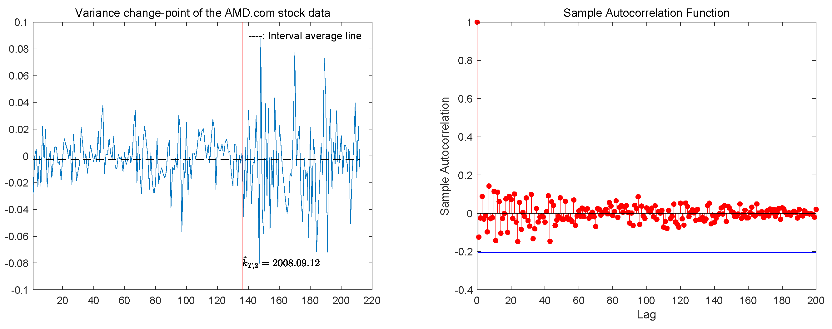
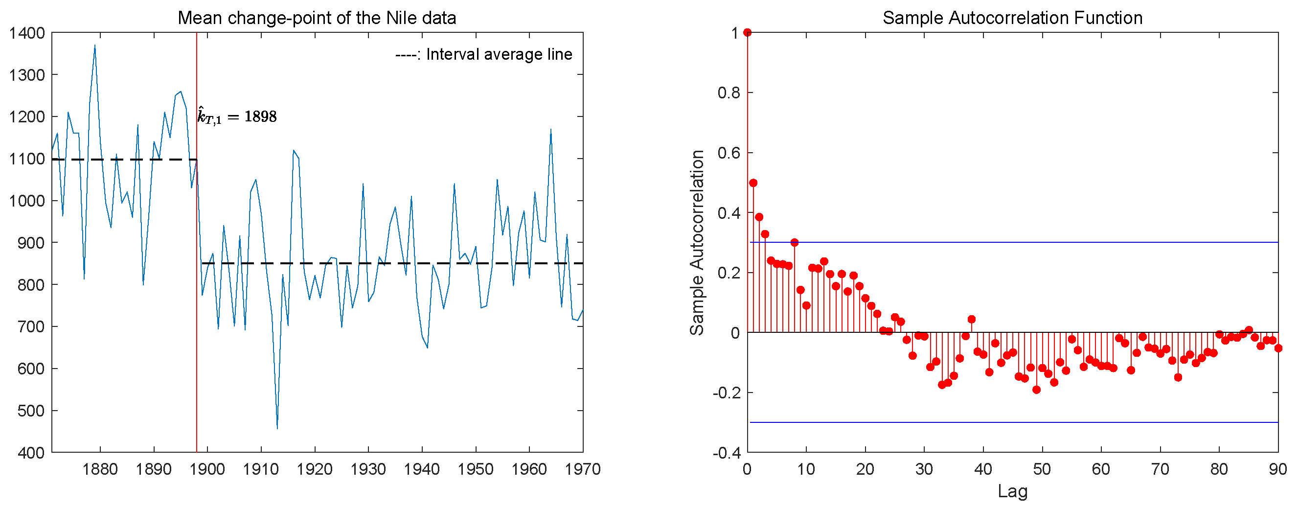
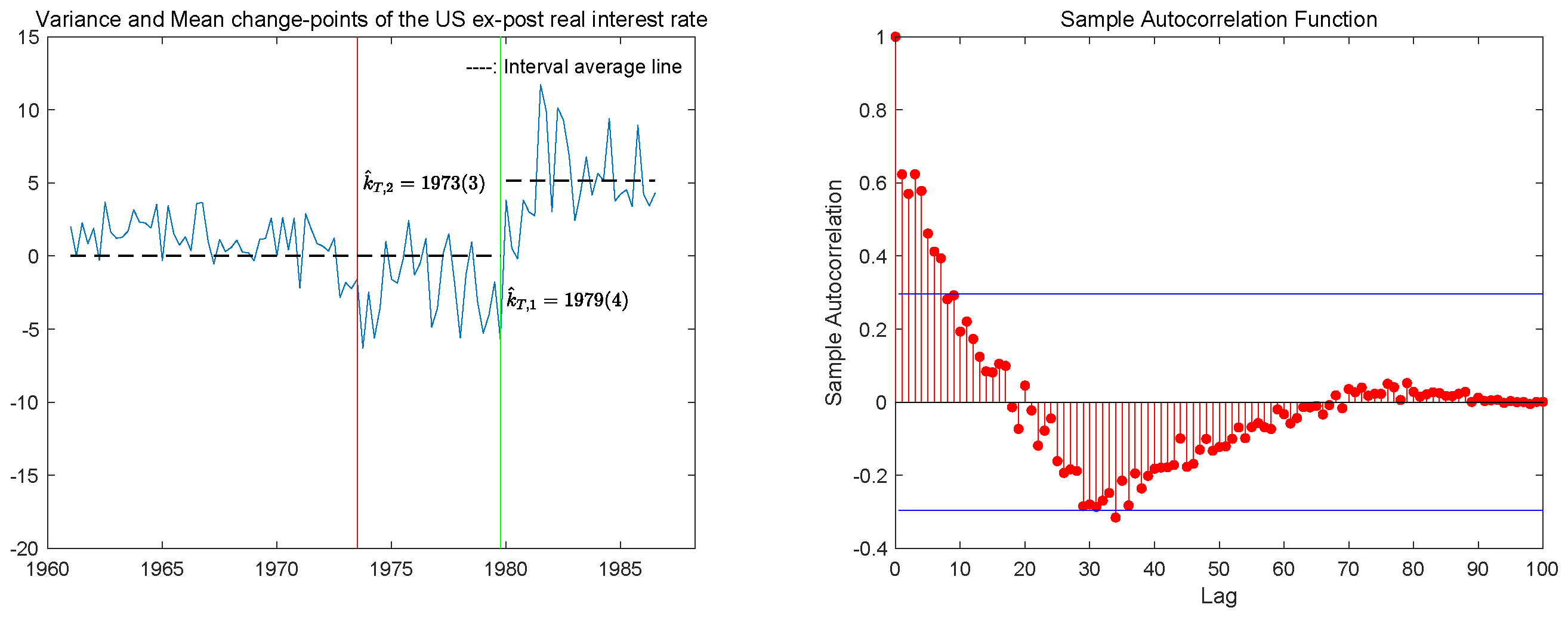
5. The Real Data Analysis

In this section, we give three examples of real data to illustrate our three-step test for the change-point detection of mean and variance. The statistics $\underset{1\le k\le T-1}{max}f{(T,k)}^{\top }f(T,k)$, $\underset{1\le k\le T-1}{max}\left|\frac{g_1(T,k)}{\sqrt{{\widehat{s}}_{T,1}^2}}\right|$ and $\underset{1\le k\le T-1}{max}|\frac{g_2(T,k)}{\sqrt{{\widehat{s}}_{T,2}^2}}|$ can be found in Section 3.

Example 1.

The dataset is the annual flow of the river Nile at Aswan from 1871 to 1970 (see [57]), and it contains 100 observations denoted by $x_t$, $1\le t\le 100$ (see Figure 1). It measures the annual discharge at Aswan in 108 $m^3$ and is depicted in Figure 1. The sample autocorrelation function (ACF) is also presented in Figure 1. By the right side of Figure 1, the autocorrelation coefficient is relatively large when the lag is small, but it approaches zero as the lag increases. Therefore, the data satisfies the properties of α-mixing. By Figure 1, it seams that there is a mean change-point in the time series of the annual flow of the river Nile.

To judge the existence of change-points, we set the null hypothesis that the annual flow of the river Nile has no change in the mean or variance. We use our three-step algorithm given in Section 3 to find the change-points. Base on $x_1,x_2,\cdots ,x_{100}$, by Step 1, we take $\alpha =0.1$, $T=100$, $h_T=\lfloor T^{1/5}\rfloor$ and obtain $\underset{1\le k\le T-1}{max}f{(T,k)}^{\top }f(T,k)=4.6048>2.054$. Therefore, we reject the null hypothesis and conclude that there is at least a change-point of mean or variance. By Step 2, it has $\underset{1\le k\le T-1}{max}|\frac{g_1(T,k)}{\sqrt{{\widehat{s}}_{T,1}^2}}|=1.7838>1.358$ and the p-value $p_{v1}=0.0034<0.05$. It means that there is a mean change-point located at ${\widehat{k}}_{T,1}=\underset{1\le k\le T-1}{argmax}|U_{k,1}|=28$. Meanwhile, it calculates by Step 3 with the modified data of the mean change that $\underset{1\le k\le T-1}{max}|\frac{g_2(T,k)}{\sqrt{{\widehat{s}}_{T,2}^2}}|=1.0415<1.358$ and the p-value $p_{v2}=0.2282>0.05$. It means that there is no evidence of a variance change-point. Consequently, we conclude that there is only one mean change-point in the time series of the annual flow of the river Nile. It is pointed out that change-point 28 is the year 1898, when the Aswan dam was built. Since the Aswan dam was built, it has significantly changed the mean annual flow of the river Nile. In addition, Zeileis et al. [58] used the F test to detect the same change-point 28. We also use the cpt.meanvar method (see [12]) and the mosum method with bandwidth $G=20$ (see [13]) from the R and obtain the same change-point 28.

Example 2.

The dataset is the prices of AMD stock downloaded by Python, which contains 212 observations from 3 March 2008 to 31 December 2008. Let $P_t$ be the closing price of AMD stock, and the return can be defined as $r_t=log{P}_t-log{P}_{t-1}$ and $P_0=1$ for $1\le t\le 212$. Figure 2 shows the plots of times series of returns of AMD stock and its sample ACF.

By the right side of Figure 2, the times series of returns satisfy the properties of α-mixing. In addition, by the left side of Figure 2, the returns are around zero, but the variance of returns seams to change. Therefore, we use the three-step algorithm to find the change-points and set the null hypothesis that the return of AMD stock has no change in mean or variance. Based on the sample $r_1,r_2,\cdots ,r_{212}$, by Step 1, we take $\alpha =0.1$, $T=212$, $h_T=\lfloor T^{1/5}\rfloor$ and obtain $\underset{1\le k\le T-1}{max}f{(T,k)}^{\top }f(T,k)=4.4340>2.054$. By Step 2, it has $\underset{1\le k\le T-1}{max}|\frac{g_1(T,k)}{\sqrt{{\widehat{s}}_{T,1}^2}}|=0.8974<1.358$ and $p_{v1}=0.3963>0.05$. It means that there is no evidence of a mean change-point. By Step 3, it has $\underset{1\le k\le T-1}{max}|\frac{g_2(T,k)}{\sqrt{{\widehat{s}}_{T,2}^2}}|=1.9398>1.358$ and $p_{v2}=0.0011<0.05$. Therefore, we detect a variance change-point located at ${\widehat{k}}_{T,2}=\underset{1\le k\le T-1}{argmax}\left|U_{k,2}\right|=136$ (on 12 September 2008). On the other hand, under the independent normal random variables, the authors investigated the change-point detection of variance [5,25]. Thus, we use the methods in [5,25] to detect the variance change-points 136 and 137, respectively. We also use the cpt.meanvar method from the R and obtain a change-point 136. However, we do not detect any change-point using the mosum method. Obviously, the difference between 136 and 137 is only one. Furthermore, it is known that Lehman Brothers declared bankruptcy on 15 September 2008, i.e., point 137. Therefore, it added financial risk to the stock market. Consequently, the variance of returns of AMD stock began to increase after the time of the bankruptcy of Lehman Brothers.

Example 3.

The dataset is the quarterly US ex-post real interest rate from 1961:Q1 to 1986:Q3 provided by Citibase data bank (see [59]). The data are also available from the R package strucchange (see [60]) and denoted by $x_t$, $1\le t\le 103$ (see Figure 3). The sample AFC based on the quarterly US ex-post real interest rate is also shown in Figure 3.

Similarly, by the right left of Figure 3, the times series of US ex-post real interest rate satisfy the properties of α-mixing; and by the left side of Figure 3, it seems that there are some change-points of mean or variance. We also use the three-step algorithm to find the change-points and set the null hypothesis that the quarterly US ex-post real interest rate has no change in mean or variance. Base on $x_1,x_2,\cdots ,x_{103}$, by $\alpha =0.1$, $T=103$, $h_T=\lfloor T^{1/5}\rfloor$ and Step 1, we have $\underset{1\le k\le T-1}{max}f{(T,k)}^{\top }f(T,k)=3.9193>2.054$. It means that there exist some change-points in this times series $\{x_1,x_2,\cdots ,x_{103}\}$. By Step 2, it has $\underset{1\le k\le T-1}{max}|\frac{g_1(T,k)}{\sqrt{{\widehat{s}}_{T,1}^2}}|=1.5973>1.358$, $p_{v1}=0.0122<0.05$. So there exists a mean change-point at ${\widehat{k}}_{T,1}=\underset{1\le k\le T-1}{argmax}|U_{k,1}|=76$ (on 1979:Q4). Then, it can be checked by Step 3 with the modified data of the mean change that $\underset{1\le k\le T-1}{max}|\frac{g_2(T,k)}{\sqrt{{\widehat{s}}_{T,2}^2}}|=1.3779>1.358$ and $p_{v2}=0.0449<0.05$. In other words, it has a variance change-point located at ${\widehat{k}}_{T,2}=\underset{1\le k\le T-1}{argmax}\left|U_{k,2}\right|=51$ (on 1973:Q3). Consequently, we detect a mean change-point 76 and a variance change-point 51. In addition, we use mosum method from the R with bandwidth $G=25$ to detect two change-points 47 and 76. Meanwhile, we apply cpt.meanvar from the R and find two change-points 47 and 79. On the other hand, the differences between the change-points $\{51,76\}$, $\{47,76\}$, $\{47,79\}$ are small. However, we detect the change-point 76 to be a mean change-point and detect point 51 to be a variance change-point, while the mosum and cpt.meanvar methods do not specify the types of these change-points. Thus, our method has an advantage over their methods. Furthermore, it is pointed out that the sudden jump in oil prices in 1973 added to the volatility of the US ex-post real interest rate. We also point out that the Federal Reserve’s operating procedures in October 1979 increased the means of US ex-post real interest rate (see [59]).

6. Conclusions

Many researchers have studied the mean change-point models and variance change-point models, and obtained the limiting distributions for the CUSUM statistics of the mean change-point and variance change-point (see [3,6]). As far as we know, there are few papers to study the change-point model with the mean change and variance change. In this paper, we consider the mean-variance change-point model (1) with the $\alpha$-mixing errors. Based on the CUSUM statistics of mean and variance, we give the combination statistic $g{(T,k)}^{\top }g(T,k)$ in (4). To determine whether there is a change-point of mean or variance, the limiting distributions for the CUSUM statistics $g{(T,k)}^{\top }g(T,k)$ and $\underset{1\le k\le T-1}{max}g{(T,k)}^{\top }g(T,k)$ are obtained under the null hypothesis there is no change in mean or variance. Some consistent estimators ${\widehat{s}}_{T,1}^2$ and ${\widehat{s}}_{T,2}^2$ for long-run variances $s_1^2$ and $s_2^2$ are presented in (17) of Lemma 1, respectively. Then, we obtain the limiting distributions for a combination statistic $\underset{1\le k\le T-1}{max}f{(T,k)}^{\top }f(T,k)$, mean CUSUM statistic $\underset{1\le k\le T-1}{max}|\frac{g_1(T,k)}{\sqrt{{\widehat{s}}_{T,1}^2}}|$ and variance CUSUM statistic $\underset{1\le k\le T-1}{max}|\frac{g_2(T,k)}{\sqrt{{\widehat{s}}_{T,2}^2}}|$ in Corollaries 1 and 2. As an application, we give a three-step algorithm for change-point detection. The first step is to test whether there is at least a change-point or not. The second step and third step are to detect the mean change-point and variance change-point, respectively. To illustrate our three-step test of the change-point detection, some simulations and three real data examples are presented in Section 4 and Section 5, respectively. It can be seen that our algorithm has an advantage over the existing methods cpt.meanvar by [12] and mosum by [13]. For example, our method not only has a high power but can also determine the change-points as the mean change-point or variance change-point. On the other hand, the multiple change-point problems of the mean, variance, mean vector, and covariance matrix have gained much attention. In this article, we consider the limit distribution under the null hypothesis of no change-point. It is important for research to investigate the limit distribution under the alternative hypotheses. It is also interesting for researchers to study these problems based on the dependent panel data, high-dimensional data, and other dependent data in future work.

7. Proofs of Main Results

Lemma 2

(Lemma 1 in [49]). Let $Y_t=g_t(e_t,\cdots ,e_{t-\tau })$, where $g_t$ is a measurable function onto $R^{\upsilon }$ and τ and υ are finite positive integers. If $\{e_t,t\ge 1\}$ is an α-mixing with $\alpha \left(t\right)=O\left(t^{-\lambda }\right)$ for some $\lambda >0$, then $\{Y_t,t\ge 1\}$ is also an α-mixing with $\alpha \left(t\right)=O\left(t^{-\lambda }\right)$.

Lemma 3

(Proposition 2.5 in [51]). Let $X\in {\mathcal{F}}_{-\infty }^k$, $Y\in {\mathcal{F}}_{k+t}^{\infty }$. If ${E\left|X\right|}^p<\infty$ and ${E\left|Y\right|}^q<\infty$ for some $p,q\ge 1$ and $1/p+1/q<1$, then

$$\left|\mathrm{Cov}(X,Y)\right|\le {8\left(\mathrm{E}\right|X|}^p{)}^{1/p}{\left(\mathrm{E}\right|Y|}^q{)}^{1/q}{\alpha }^{1-1/p-1/q}\left(t\right).$$

Lemma 4

(Lemma 1.4 in [52]). For some $\delta >0$, let $\{e_t,t\ge 1\}$ be a mean zero α-mixing sequence with $E|e_t{|}^{2+\delta }<\infty$ for all $t\ge 1$ and ${\sum }_{t=1}^{\infty }{\alpha }^{\frac{\delta }{2+\delta }}\left(t\right)<\infty$. Then

$$\mathrm{E}{(\sum _{t=1}^T{e}_t)}^2\le [1+16\sum _{t=1}^{\infty }{\alpha }^{\frac{\delta }{2+\delta }}\left(t\right)]\sum _{t=1}^T\left(\mathrm{E}\right|e_t{{|}^{2+\delta })}^{\frac{2}{2+\delta }},T\ge 1.$$

Lemma 5

(Corollary 1 in [47] and Theorem 0 in [48]). For some $\delta >0$, let $\{e_t,t\ge 1\}$ be an α-mixing sequence with $E{e}_t=0$ for all $t\ge 1$, $\underset{t\ge 1}{sup}\mathrm{E}{\left|e_t\right|}^{2+\delta }<\infty$ and ${\sum }_{t=1}^{\infty }{\alpha }^{\frac{\delta }{2+\delta }}\left(t\right)<\infty$. For $T\ge 1$, denote $S_T={\sum }_{t=1}^T{e}_t$ and suppose

$$\mathrm{E}{S}_T^2/T\to {\sigma }^2>0,\mathrm{as}T\to \infty .$$

Then

$$\frac{S_T}{\sqrt{T{\sigma }^2}}\stackrel{d}{⟶}N(0,1),\mathrm{as}T\to \infty .$$

(28)

Furthermore,

$$W_T\left(x\right)\Rightarrow W\left(x\right),\mathrm{as}T\to \infty ,$$

(29)

where $W_T\left(x\right)=S_{\lfloor Tx\rfloor }/\sqrt{T{\sigma }^2}$ for $x\in [0,1]$, and $\left\{W\right(x),x\in [0,1\left]\right\}$ is a Wiener process(standard Brownian motion). Then, for $\forall x\in [0,1]$,

$$W_T\left(x\right)-x{W}_T\left(1\right)\Rightarrow W\left(x\right)-xW\left(1\right)\sim W^0\left(x\right),asT\to \infty ,$$

(30)

where $\{W^0\left(x\right);x\in [0,1]\}$ is a standard Brownian bridge.

Lemma 6.

Let the Assumptions 1 and 2 be satisfied. Denote

$${\xi }_T=\frac{{\sigma }_0}{\sqrt{T{s}_1^2}}\sum _{t=1}^T{e}_{t}and{\eta }_T=\frac{{\sigma }_0^2}{\sqrt{T{s}_2^2}}\sum _{t=1}^T(e_t^2-\mathrm{E}{e}_t^2),$$

where ${\sigma }_0$ is defined by (5), $s_1^2$ and $s_2^2$ are defined by (10), respectively. Under the null hypothesis $H_0$ defined by (5), it has

$$({\xi }_T,{\eta }_T)\stackrel{d}{⟶}(\xi ,\eta ),asT\to \infty ,$$

(31)

where ξ and η are two independent $N(0,1)$ random variables. For some $x\in [0,1]$, let $k=\lfloor xT\rfloor$. Then

$$(\frac{{\sigma }_0}{\sqrt{T{s}_1^2}}\sum _{t=1}^k{e}_t,\frac{{\sigma }_0^2}{\sqrt{T{s}_2^2}}\sum _{t=1}^k(e_t^2-\mathrm{E}{e}_t^2))\Rightarrow (W_1\left(x\right),W_2\left(x\right)),$$

(32)

and

$$(\frac{{\sigma }_0}{\sqrt{T{s}_1^2}}(\sum _{t=1}^k{e}_t-\frac{k}{T}\sum _{t=1}^T{e}_t),\frac{{\sigma }_0^2}{\sqrt{T{s}_2^2}}(\sum _{t=1}^k{e}_t^2-\frac{k}{T}\sum _{t=1}^T{e}_t^2))\Rightarrow (W_1^0\left(x\right),W_2^0\left(x\right)),$$

(33)

where $W_1^0\left(x\right)$ and $W_2^0\left(x\right)$ are independent standard Brownian bridge.

Proof of Theorem 1.

By (1), (2), (4), (5) and $\mathrm{E}{e}_t=0$ for all $t\ge 1$, it is easy to check that

$$\begin{array}{ccc}\hfill \frac{g_1(T,k)}{\sqrt{s_1^2}}& =& \frac{1}{\sqrt{T{s}_1^2}}{U}_{k,1}=\frac{1}{\sqrt{T{s}_1^2}}(\frac{k(T-k)}{T})(\frac{1}{k}\sum _{t=1}^k{X}_t-\frac{1}{T-k}\sum _{t=k+1}^T{X}_t)\hfill \\ & =& \frac{1}{\sqrt{T{s}_1^2}}(\sum _{t=1}^k{X}_t-\frac{k}{T}\sum _{t=1}^T{X}_t)=\frac{{\sigma }_0}{\sqrt{T{s}_1^2}}(\sum _{t=1}^k{e}_t-\frac{k}{T}\sum _{t=1}^T{e}_t).\hfill \end{array}$$

(34)

Meanwhile, it has

$$\begin{array}{ccc}& & \frac{1}{k}\sum _{t=1}^k{(X_t-\overline{X})}^2-\frac{1}{T-k}\sum _{t=k+1}^T{(X_t-\overline{X})}^2\hfill \\ & =& \frac{1}{k}\sum _{t=1}^k(X_t^2-2X_t\overline{X}+{\overline{X}}^2)-\frac{1}{T-k}\sum _{t=k+1}^T(X_t^2-2X_t\overline{X}+{\overline{X}}^2)\hfill \\ & =& (\frac{1}{k}\sum _{t=1}^k{X}_t^2-\frac{1}{T-k}\sum _{t=k+1}^T{X}_t^2)-2\overline{X}(\frac{1}{k}\sum _{t=1}^k{X}_t-\frac{1}{T-k}\sum _{t=k+1}^T{X}_t)\hfill \\ & =& (\frac{1}{k}\sum _{t=1}^k{({\mu }_0+{\sigma }_0{e}_t)}^2-\frac{1}{T-k}\sum _{t=k+1}^T{({\mu }_0+{\sigma }_0{e}_t)}^2)\hfill \\ & & -2\overline{X}(\frac{1}{k}\sum _{t=1}^k({\mu }_0+{\sigma }_0{e}_t)-\frac{1}{T-k}\sum _{t=k+1}^T({\mu }_0+{\sigma }_0{e}_t))\hfill \\ & =& 2{\sigma }_0({\mu }_0-\overline{X})(\frac{1}{k}\sum _{t=1}^k{e}_t-\frac{1}{T-k}\sum _{t=k+1}^T{e}_t)+{\sigma }_0^2(\frac{1}{k}\sum _{t=1}^k{e}_t^2-\frac{1}{T-k}\sum _{t=k+1}^T{e}_t^2),\hfill \end{array}$$

where $\overline{X}=\frac{1}{T}{\sum }_{t=1}^T{X}_t$. Combining this with (4), we have

$$\begin{array}{ccc}\hfill \frac{g_2(T,k)}{\sqrt{s_2^2}}& =& \frac{1}{\sqrt{T{s}_2^2}}{U}_{k,2}\hfill \\ & =& \frac{1}{\sqrt{T{s}_2^2}}(\frac{k(T-k)}{T})[2{\sigma }_0({\mu }_0-\overline{X})(\frac{1}{k}\sum _{t=1}^k{e}_t-\frac{1}{T-k}\sum _{t=k+1}^T{e}_t)\hfill \\ & & +{\sigma }_0^2(\frac{1}{k}\sum _{t=1}^k{e}_t^2-\frac{1}{T-k}\sum _{t=k+1}^T{e}_t^2)]\hfill \\ & =& \frac{2{\sigma }_0({\mu }_0-\overline{X})}{\sqrt{T{s}_2^2}}(\sum _{t=1}^k{e}_t-\frac{k}{T}\sum _{t=1}^T{e}_t)+\frac{{\sigma }_0^2}{\sqrt{T{s}_2^2}}(\sum _{t=1}^k{e}_t^2-\frac{k}{T}\sum _{t=1}^T{e}_t^2)\hfill \\ & :=& D_{T1}+D_{T2}.\hfill \end{array}$$

(35)

By $\delta >0$ and $\underset{t\ge 1}{sup}\mathrm{E}{\left|e_t\right|}^{4+2\delta }<\infty$, it has $\underset{t\ge 1}{sup}\mathrm{E}{\left|e_t\right|}^{2+\delta }<\infty$. Then, by Lemma 4 with $\underset{t\ge 1}{sup}\mathrm{E}{\left|e_t\right|}^{2+\delta }<\infty$ and ${\sum }_{t=1}^{\infty }{\alpha }^{\frac{\delta }{2+\delta }}\left(t\right)<\infty$, it has

$$\begin{array}{ccc}\hfill \mathrm{Var}\left(\overline{X}\right)& =& \mathrm{E}{(\overline{X}-{\mu }_0)}^2\hfill \\ & =& \frac{{\sigma }_0^2}{T^2}E{(\sum _{t=1}^T{e}_t)}^2\le \frac{C_1}{T^2}(1+16\sum _{t=1}^{\infty }{\alpha }^{\frac{\delta }{2+\delta }}\left(t\right))\sum _{t=1}^T{(\mathrm{E}|e_t{|}^{2+\delta })}^{\frac{2}{2+\delta }}=O(\frac{1}{T}),\hfill \end{array}$$

(36)

which implies

$$\overline{X}-{\mu }_0=O_P\left(T^{-1/2}\right).$$

(37)

In addition, we apply (33) in Lemma 6 and obtain that

$$\frac{2{\sigma }_0}{\sqrt{T{s}_2^2}}(\sum _{t=1}^k{e}_t-\frac{k}{T}\sum _{t=1}^T{e}_t)=O_P\left(1\right).$$

Thus, it has $D_{T1}=O_P\left(T^{-1/2}\right)=o_P\left(1\right)$, which implies that $D_{T2}$ in (35) is a main term. Last, by (34) and (35) and $D_{T1}=o_P\left(1\right)$, we apply Lemma 6 and obtain (12), i.e.,

$$(\frac{g_1(T,k)}{\sqrt{s_1^2}},\frac{g_2(T,k)}{\sqrt{s_2^2}})\Rightarrow (W_1^0\left(x\right),W_2^0\left(x\right)),$$

where $W_1^0\left(x\right)$ and $W_2^0\left(x\right)$ are independent Brownian motions. In addition, by (12) and the continuous mapping theorem, (13) is also proved. □

Proof of Lemma 1.

First, we prove that $s_1^2$ in (10) absolutely converges. Obviously, $\mathrm{E}|e_1{|}^{8+4\delta }<\infty$ implies $\mathrm{E}|e_1{|}^{2+\delta }<\infty$ for some $\delta >0$. Then, by the second-order stationarity of $\alpha$-mixing sequence $\{e_t,t\ge 1\}$, we apply Lemma 3 with $\mathrm{E}{e}_1=0$, $\mathrm{E}{e}_1^2=1$, $\mathrm{E}|e_1{|}^{2+\delta }<\infty$ and ${\sum }_{t=1}^{\infty }{\alpha }^{\frac{\delta }{2+\delta }}\left(t\right)<\infty$, and obtain that

$$\begin{array}{ccc}\hfill 0& <& s_1^2={\gamma }_1\left(0\right)+2\sum _{h=1}^{\infty }{\gamma }_1\left(h\right)\le \mathrm{Var}\left(X_1\right)+2\sum _{h=1}^{\infty }\left|\mathrm{Cov}(X_1,X_{1+h})\right|\hfill \\ & \le & {\sigma }_0^2[\mathrm{Var}\left(e_1\right)+2\sum _{h=1}^{\infty }\left|\mathrm{Cov}(e_1,e_{1+h})\right|]<\infty .\hfill \end{array}$$

(38)

By (10) and (16), we use the decomposition

$$|{\widehat{s}}_{T,1}^2-s_1^2|\le |{\widehat{\gamma }}_1\left(0\right)-{\gamma }_1\left(0\right)|+2\sum _{h=1}^{h_T}|{\widehat{\gamma }}_1\left(h\right)-{\gamma }_1\left(h\right)|+2\sum _{h=h_T+1}^{\infty }\left|{\gamma }_1\left(h\right)\right|:=\sum _{i=1}^3{K}_{T,i},$$

(39)

where $h_T\to \infty$ as $T\to \infty$.

Obviously, by (38), (39) and $h_T\to \infty$ as $T\to \infty$, it can be checked that

$$K_{T,3}\to 0,\mathrm{as}T\to \infty .$$

(40)

Now, we consider the term $K_{T,1}$ in (39). Obviously, by the second-order stationarity of $\left\{e_t\right\}$, (14), $\mathrm{E}{e}_1=0$ and ${\gamma }_1\left(0\right)={\sigma }_0^2\mathrm{E}{e}_1^2$, we obtain that

$${\widehat{\gamma }}_1\left(0\right)-{\gamma }_1\left(0\right)=\frac{{\sigma }_0^2}{T}\sum _{t=1}^T(e_t^2-\mathrm{E}{e}_t^2)-{\sigma }_0^2{\left(\overline{e}\right)}^2,$$

(41)

where $\overline{e}=\frac{1}{T}{\sum }_{t=1}^T{e}_t=\frac{\overline{X}-{\mu }_0}{{\sigma }_0}$. Combining with (37), we have

$$\begin{array}{c}\hfill \overline{e}=O_P\left(T^{-1/2}\right).\end{array}$$

(42)

By $\mathrm{E}|e_1{|}^{8+4\delta }<\infty$, it has $\mathrm{E}|e_1{|}^{2(2+\delta )}<\infty$ for some $\delta >0$. In addition by the second-order stationarity of $\alpha$-mixing sequence $\{(e_t^2-\mathrm{E}{e}_t^2),t\ge 1\}$ with $\mathrm{E}(e_1^2-\mathrm{E}{e}_1^2)=0$, $\mathrm{E}|e_1^2-\mathrm{E}{e}_1^2{|}^{2+\delta }<\infty$ and ${\sum }_{t=1}^{\infty }{\alpha }^{\frac{\delta }{2+\delta }}\left(t\right)<\infty$, we apply Lemma 4 and obtain that

$$\mathrm{E}|\sum _{t=1}^T(e_t^2-\mathrm{E}{e}_t^2){|}^2\le (1+16\sum _{t=1}^{\infty }{\alpha }^{\frac{\delta }{2+\delta }}\left(t\right))\sum _{t=1}^T{\left(\mathrm{E}{(e_t^2-\mathrm{E}{e}_t^2)}^{2+\delta }\right)}^{\frac{2}{2+\delta }}=O\left(T\right),$$

(43)

which implies

$$|\sum _{t=1}^T(e_t^2-\mathrm{E}{e}_t^2)|=O_P\left(T^{1/2}\right),$$

(44)

Consequently, it follows from (41), (42), (44) and $0<{\sigma }_0^2<\infty$ that

$$|{\widehat{\gamma }}_1\left(0\right)-{\gamma }_1\left(0\right)|\le {\sigma }_0^2|\frac{1}{T}\sum _{t=1}^T(e_t^2-\mathrm{E}{e}_t^2)|+{\sigma }_0^2{\left(\overline{e}\right)}^2=O_P(T^{-\frac{1}{2}})+O_P\left(T^{-1}\right)=O_P(T^{-\frac{1}{2}}).$$

(45)

Thus, it has

$$K_{T,1}=o_P\left(1\right).$$

(46)

Next, we consider $K_{T,2}$. By (14), $\mathrm{E}{e}_1=0$, ${\gamma }_1\left(h\right)={\sigma }_0^2\mathrm{E}{e}_1{e}_{1+h}$ and

$${\widehat{\gamma }}_1\left(h\right)={\sigma }_0^2[\frac{1}{T}\sum _{t=1}^{T-h}{e}_t{e}_{t+h}-2{\left(\overline{e}\right)}^2+\frac{T-h}{T}{\left(\overline{e}\right)}^2+\frac{\overline{e}}{T}\sum _{t=T-h+1}^T{e}_t+\frac{\overline{e}}{T}\sum _{t=1}^h{e}_t],$$

it can be seen that

$$\begin{array}{ccc}\hfill {\widehat{\gamma }}_1\left(h\right)-{\gamma }_1\left(h\right)& =& {\sigma }_0^2[\frac{1}{T}\sum _{t=1}^{T-h}(e_t{e}_{t+h}-\mathrm{E}{e}_t{e}_{t+h})-\frac{1}{T}\sum _{t=T-h+1}^T\mathrm{E}{e}_t{e}_{t+h}\hfill \\ & & -(\frac{h}{T}+1){\left(\overline{e}\right)}^2+\frac{\overline{e}}{T}\sum _{t=T-h+1}^T{e}_t+\frac{\overline{e}}{T}\sum _{t=1}^h{e}_t]\hfill \\ & :=& {\sigma }_0^2\sum _{i=1}^5{N}_{h,i}.\hfill \end{array}$$

(47)

By Lemma 3, it can be seen that $\{e_t{e}_{t+h},1\le t\le T-h\}$ are $\alpha$-mixing random variables with the same mixing coefficients. Thus, by Lemma 4 with $\mathrm{E}|e_1{|}^{2(2+\delta )}<\infty$ and ${\sum }_{t=1}^{\infty }{\alpha }^{\frac{\delta }{2+\delta }}\left(t\right)<\infty$, we establish that

$$\mathrm{E}{(\sum _{t=1}^{T-h}[e_t{e}_{t+h}-\mathrm{E}\left(e_t{e}_{t+h}\right)])}^2\le C_1\sum _{t=1}^{T-h}{\left(E{[\left(e_t{e}_{t+h}\right)-\mathrm{E}\left(e_t{e}_{t+h}\right)]}^{2+\delta }\right)}^{\frac{2}{2+\delta }}=O(T-h),$$

which implies

$$|\sum _{t=1}^{T-h}[e_t{e}_{t+h}-\mathrm{E}\left(e_t{e}_{t+h}\right)]|=O_P\left(\sqrt{T-h}\right)=O_P\left(T^{1/2}\right).$$

(48)

By (47) and (48) and the fact $h_T=O\left(T^{\beta }\right)$ in (11) and $\beta \in (0,1/2)$, we obtain that

$$\sum _{h=1}^{h_T}\left|N_{h,1}\right|=O_P\left(T^{\beta -1/2}\right)=o_P\left(1\right).$$

(49)

Meanwhile, by $\mathrm{E}{e}_1^2<\infty$, Hölder inequality and $0<\beta <1/2$, it has

$$\sum _{h=1}^{h_T}\left|N_{h,2}\right|\le \frac{1}{T}\sum _{h=1}^{h_T}\sum _{t=T-h+1}^T{\left(\mathrm{E}{e}_t^2\right)}^{1/2}{\left(\mathrm{E}{e}_{t+h}^2\right)}^{1/2}\le \frac{C}{T}\sum _{h=1}^{h_T}h=O\left(T^{2\beta -1}\right)=o\left(1\right).$$

(50)

By (42),

$$\sum _{h=1}^{h_T}\left|N_{h,3}\right|\le \sum _{h=1}^{h_T}(\frac{h}{T}+1){\left(\overline{e}\right)}^2=O_P\left(T^{\beta -1}\right)=o_P\left(1\right).$$

(51)

Similar to the proof of (44), we have

$$|\sum _{t=T-h+1}^T{e}_t|=O_P\left(\sqrt{h}\right).$$

(52)

Thus, it follows from (42), (47), (52), $h_T=O\left(T^{\beta }\right)$ and $\beta \in (0,1/2)$ that

$$\begin{array}{c}\hfill \sum _{h=1}^{h_T}\left|N_{h,4}\right|\le \frac{|\overline{e}|}{T}\sum _{h=1}^{h_T}|\sum _{t=T-h+1}^T{e}_t|=O_P\left(T^{-3/2}\right)O_P\left(h_T^{3/2}\right)=O_P\left(T^{3(\beta -1)/2}\right)=o_P\left(1\right).\end{array}$$

(53)

Similarly,

$$\sum _{h=1}^{h_T}\left|N_{h,5}\right|=O_P\left(T^{3(\beta -1)/2}\right)=o_P\left(1\right).$$

(54)

Therefore, by (39), (47), (49)–(54) and $0<{\sigma }_0^2<\infty$, we establish

$$K_{T,2}\le 2{\sigma }_0^2\sum _{h=1}^{h_T}\sum _{i=1}^5\left|N_{h,i}\right|=o_P\left(1\right).$$

(55)

Finally, it follows from (39), (40), (46) and (55) that

$$|{\widehat{s}}_{T,1}^2-s_1^2|=o_P\left(1\right),$$

(56)

i.e., the first term in (17) is proved.

Next, we prove the right of (17). Similar to (39), by (10) and (16), it follows

$$|{\widehat{s}}_{T,2}^2-s_2^2|\le |{\widehat{\gamma }}_2\left(0\right)-{\gamma }_2\left(0\right)|+2\sum _{h=1}^{h_T}|{\widehat{\gamma }}_2\left(h\right)-{\gamma }_2\left(h\right)|+2\sum _{h=h_T+1}^{\infty }\left|{\gamma }_2\left(h\right)\right|:=\sum _{i=1}^3{R}_{T,i},$$

(57)

where $h_T\to \infty$ as $T\to \infty$. Similar to the proof of (38), by Lemma 3 with $\mathrm{E}|e_1{|}^{2(2+\delta )}<\infty$ and ${\sum }_{t=1}^{\infty }{\alpha }^{\frac{\delta }{2+\delta }}\left(t\right)<\infty$, it follows

$$\begin{array}{ccc}\hfill 0& <& s_2^2={\gamma }_2\left(0\right)+2\sum _{h=1}^{\infty }{\gamma }_2\left(h\right)\le \mathrm{Var}\left({(X_1-{\mu }_0)}^2\right)+2\sum _{h=1}^{\infty }\mathrm{Cov}({(X_1-{\mu }_0)}^2,{(X_{1+h}-{\mu }_0)}^2)\hfill \\ & \le & {\sigma }_0^4(\mathrm{Var}\left(e_1^2\right)+2\sum _{h=1}^{\infty }\left|\mathrm{Cov}(e_1^2,e_{1+h}^2)\right|)<\infty .\hfill \end{array}$$

Thus, we have

$$R_{T,3}\to 0,\mathrm{as}T\to \infty$$

(58)

proving $h_T\to \infty$ as $T\to \infty$.

Now, we consider the term $R_{T,1}$ in (57). By (15) and

$${\gamma }_2\left(0\right)=\mathrm{E}{(X_1-{\mu }_0)}^4-{\left(\mathrm{E}{(X_1-{\mu }_0)}^2\right)}^2,$$

we obtain

$$\begin{array}{ccc}& & {\widehat{\gamma }}_2\left(0\right)-{\gamma }_2\left(0\right)\hfill \\ & =& \frac{1}{T}\sum _{t=1}^T{(X_t-{\mu }_0)}^4+\frac{4({\mu }_0-\overline{X})}{T}\sum _{t=1}^T{(X_t-{\mu }_0)}^3+\frac{8{({\mu }_0-\overline{X})}^2}{T}\sum _{t=1}^T{(X_t-{\mu }_0)}^2\hfill \\ & & +\frac{4{({\mu }_0-\overline{X})}^3}{T}\sum _{t=1}^T(X_t-{\mu }_0)-{(\frac{1}{T}\sum _{t=1}^T{(X_t-{\mu }_0)}^2)}^2-\mathrm{E}{(X_1-{\mu }_0)}^4+{\left(\mathrm{E}{(X_1-{\mu }_0)}^2\right)}^2\hfill \\ & =& \frac{1}{T}\sum _{t=1}^T\left[{(X_t-{\mu }_0)}^4-\mathrm{E}{(X_t-{\mu }_0)}^4\right]+\frac{4({\mu }_0-\overline{X})}{T}\sum _{t=1}^T\left[{(X_t-{\mu }_0)}^3-\mathrm{E}{(X_t-{\mu }_0)}^3\right]\hfill \\ & & +\frac{8{({\mu }_0-\overline{X})}^2}{T}\sum _{t=1}^T\left[{(X_t-{\mu }_0)}^2-\mathrm{E}{(X_t-{\mu }_0)}^2\right]+\frac{4{({\mu }_0-\overline{X})}^3}{T}\sum _{t=1}^T\left[(X_t-{\mu }_0)-\mathrm{E}(X_t-{\mu }_0)\right]\hfill \\ & & -{\{\frac{1}{T}\sum _{t=1}^T\left[{(X_t-{\mu }_0)}^2-\mathrm{E}{(X_t-{\mu }_0)}^2+\mathrm{E}{(X_t-{\mu }_0)}^2\right]\}}^2\hfill \\ & & +4({\mu }_0-\overline{X})\mathrm{E}{(X_1-{\mu }_0)}^3+8{({\mu }_0-\overline{X})}^2\mathrm{E}{(X_1-{\mu }_0)}^2\hfill \\ & & +4{({\mu }_0-\overline{X})}^3\mathrm{E}(X_1-{\mu }_0)+{\left(\mathrm{E}{(X_1-{\mu }_0)}^2\right)}^2\hfill \\ & =& \frac{1}{T}\sum _{t=1}^T\left[{(X_t-{\mu }_0)}^4-\mathrm{E}{(X_t-{\mu }_0)}^4\right]+\frac{4({\mu }_0-\overline{X})}{T}\sum _{t=1}^T[{(X_t-{\mu }_0)}^3-\mathrm{E}{(X_t-{\mu }_0)}^3]\hfill \\ & & +\frac{8{({\mu }_0-\overline{X})}^2}{T}\sum _{t=1}^T\left[{(X_t-{\mu }_0)}^2-\mathrm{E}{(X_t-{\mu }_0)}^2\right]+\frac{4{({\mu }_0-\overline{X})}^3}{T}\sum _{t=1}^T\left[(X_t-{\mu }_0)-\mathrm{E}(X_t-{\mu }_0)\right]\hfill \\ & & -{(\frac{1}{T}\sum _{t=1}^T\left[{(X_t-{\mu }_0)}^2-\mathrm{E}{(X_t-{\mu }_0)}^2\right])}^2-\frac{2\mathrm{E}{(X_1-{\mu }_0)}^2}{T}\sum _{t=1}^T\left[{(X_t-{\mu }_0)}^2-\mathrm{E}{(X_t-{\mu }_0)}^2\right]\hfill \\ & & +4({\mu }_0-\overline{X})\mathrm{E}{(X_1-{\mu }_0)}^3+8{({\mu }_0-\overline{X})}^2\mathrm{E}{(X_1-{\mu }_0)}^2+4{({\mu }_0-\overline{X})}^3\mathrm{E}(X_1-{\mu }_0)\hfill \\ & :=& \sum _{i=1}^9{L}_{T,i}.\hfill \end{array}$$

(59)

By the null hypothesis $H_0$ defined by (5), it has $X_t={\mu }_0+{\sigma }_0{e}_t$, $t\ge 1$. Then, $\{{(X_t-{\mu }_0)}^j-\mathrm{E}{(X_t-{\mu }_0)}^j,1\le i\le T,j=1,2,3,4\}$ are also $\alpha$-mixing random variables with the same mixing coefficients. Similar to the proof of (43), by Lemma 4 with $\mathrm{E}|e_1{|}^{4(2+\delta )}<\infty$ and ${\sum }_{t=1}^{\infty }{\alpha }^{\frac{\delta }{2+\delta }}\left(t\right)<\infty$, it can be obtained

$$\begin{array}{c}\hfill \mathrm{E}{(\sum _{t=1}^T[{(X_t-{\mu }_0)}^j-\mathrm{E}{(X_t-{\mu }_0)}^j])}^2=O\left(T\right),j=1,2,3,4,\end{array}$$

(60)

which implies

$$\begin{array}{c}\hfill |\sum _{t=1}^T[{(X_t-{\mu }_0)}^j-\mathrm{E}{(X_t-{\mu }_0)}^j]|=O_P(T^{\frac{1}{2}}),j=1,2,3,4.\end{array}$$

(61)

Thus, by (37) and (61), we can obtain that

$$\begin{array}{ccc}\hfill |L_{T,1}|& =& O_P(T^{-\frac{1}{2}}),|L_{T,2}|=O_P\left(T^{-1}\right),\left|L_{T,3}\right|=O_P\left(T^{-3/2}\right),\hfill \end{array}$$

(62)

$$\begin{array}{ccc}\hfill |L_{T,4}|& =& O_P\left(T^{-2}\right),|L_{T,5}|=O_P\left(T^{-1}\right),\left|L_{T,6}\right|=O_P\left(T^{-1/2}\right),\hfill \end{array}$$

(63)

$$\begin{array}{ccc}\hfill |L_{T,7}|& =& O_P\left(T^{-1/2}\right),|L_{T,8}|=O_P\left(T^{-1}\right),\left|L_{T,9}\right|=O_P\left(T^{-3/2}\right).\hfill \end{array}$$

(64)

By (57), (59), (62)–(64), we have that

$$R_{T,1}=|{\widehat{\gamma }}_2\left(0\right)-{\gamma }_2\left(0\right)|\le \sum _{i=1}^9\left|L_{T,i}\right|=O_P(T^{-\frac{1}{2}})=o_P\left(1\right).$$

(65)

It is time to consider the term $R_{T,2}$. We can check that

$$\begin{array}{ccc}\hfill {\widehat{\gamma }}_2\left(h\right)& =& \frac{1}{T}\sum _{t=1}^{T-h}{Z}_t^2{Z}_{t+h}^2-(\frac{T+h}{T}){\left(\overline{Z^2}\right)}^2+\frac{\overline{Z^2}}{T}\sum _{t=T-h+1}^T{Z}_t^2+\frac{\overline{Z^2}}{T}\sum _{t=1}^h{Z}_t^2\hfill \\ & :=& \sum _{i=1}^4{H}_{h,i},\hfill \end{array}$$

(66)

where $Z_t=X_t-\overline{X}$. Combining with ${\gamma }_2\left(h\right)=\mathrm{E}{(X_1-{\mu }_0)}^2{(X_{1+h}-{\mu }_0)}^2-\mathrm{E}{(X_1-{\mu }_0)}^2\mathrm{E}{(X_{1+h}-{\mu }_0)}^2$, it can be checked that

$$\begin{array}{ccc}& & {\widehat{\gamma }}_2\left(h\right)-{\gamma }_2\left(h\right)\hfill \\ & =& \sum _{i=1}^4{H}_{n,i}-\mathrm{E}{(X_1-{\mu }_0)}^2{(X_{1+h}-{\mu }_0)}^2+\mathrm{E}{(X_1-{\mu }_0)}^2\mathrm{E}{(X_{1+h}-{\mu }_0)}^2\hfill \\ & =& \frac{1}{T}\sum _{t=1}^{T-h}[{(X_t-{\mu }_0)}^2{(X_{t+h}-{\mu }_0)}^2-\mathrm{E}{(X_t-{\mu }_0)}^2{(X_{t+h}-{\mu }_0)}^2]\hfill \\ & & +\frac{2({\mu }_0-\overline{X})}{T}\sum _{t=1}^{T-h}[{(X_t-{\mu }_0)}^2(X_{t+h}-{\mu }_0)-\mathrm{E}{(X_t-{\mu }_0)}^2(X_{t+h}-{\mu }_0)]\hfill \\ & & +\frac{{({\mu }_0-\overline{X})}^2}{T}\sum _{t=1}^{T-h}[{(X_t-{\mu }_0)}^2-\mathrm{E}{(X_t-{\mu }_0)}^2]\hfill \\ & & +\frac{2({\mu }_0-\overline{X})}{T}\sum _{t=1}^{T-h}[(X_t-{\mu }_0){(X_{t+h}-{\mu }_0)}^2-\mathrm{E}(X_t-{\mu }_0){(X_{t+h}-{\mu }_0)}^2]\hfill \\ & & +\frac{4{({\mu }_0-\overline{X})}^2}{T}\sum _{t=1}^{T-h}[(X_t-{\mu }_0)(X_{t+h}-{\mu }_0)-\mathrm{E}(X_t-{\mu }_0)(X_{t+h}-{\mu }_0)]\hfill \\ & & +\frac{2{({\mu }_0-\overline{X})}^3}{T}\sum _{t=1}^{T-h}(X_t-{\mu }_0)+\frac{{({\mu }_0-\overline{X})}^2}{T}\sum _{t=1}^{T-h}[{(X_{t+h}-{\mu }_0)}^2-\mathrm{E}{(X_{t+h}-{\mu }_0)}^2]\hfill \\ & & +\frac{2{({\mu }_0-\overline{X})}^3}{T}\sum _{t=1}^{T-h}(X_{t+h}-{\mu }_0)-(\frac{T+h}{T}){(\frac{1}{T}\sum _{t=1}^T[{(X_t-{\mu }_0)}^2-\mathrm{E}{(X_t-{\mu }_0)}^2])}^2\hfill \\ & & +\frac{2[{({\mu }_0-\overline{X})}^2-\mathrm{E}{(X_1-{\mu }_0)}^2](T+h)}{T^2}\sum _{t=1}^T[{(X_t-{\mu }_0)}^2-\mathrm{E}{(X_t-{\mu }_0)}^2]\hfill \\ & & +\frac{1}{T^2}\sum _{t=1}^T[{(X_t-{\mu }_0)}^2-\mathrm{E}{(X_t-{\mu }_0)}^2]\sum _{t=T-h+1}^T[{(X_t-{\mu }_0)}^2-\mathrm{E}{(X_t-{\mu }_0)}^2]\hfill \\ & & +\frac{2h\mathrm{E}{(X_1-{\mu }_0)}^2}{T^2}\sum _{t=1}^T[{(X_t-{\mu }_0)}^2-\mathrm{E}{(X_t-{\mu }_0)}^2]\hfill \\ & & +\frac{\mathrm{E}{(X_1-{\mu }_0)}^2}{T}\sum _{t=T-h+1}^T[{(X_t-{\mu }_0)}^2-\mathrm{E}{(X_t-{\mu }_0)}^2]\hfill \\ & & +\frac{2({\mu }_0-\overline{X})}{T^2}\sum _{t=1}^T[{(X_t-{\mu }_0)}^2-\mathrm{E}{(X_t-{\mu }_0)}^2]\sum _{t=T-h+1}^T(X_t-{\mu }_0)\hfill \\ & & +\frac{2({\mu }_0-\overline{X})\mathrm{E}{(X_1-{\mu }_0)}^2}{T}\sum _{t=T-h+1}^T(X_t-{\mu }_0)+\frac{2{({\mu }_0-\overline{X})}^{2}h}{T^2}\sum _{t=1}^T[{(X_t-{\mu }_0)}^2-\mathrm{E}{(X_t-{\mu }_0)}^2]\hfill \\ & & -\frac{{({\mu }_0-\overline{X})}^2}{T}\sum _{t=T-h+1}^T[{(X_t-{\mu }_0)}^2-\mathrm{E}{(X_t-{\mu }_0)}^2]-\frac{2{({\mu }_0-\overline{X})}^3}{T}\sum _{t=T-h+1}^T(X_t-{\mu }_0)\hfill \\ & & +\frac{1}{T^2}\sum _{t=1}^T[{(X_t-{\mu }_0)}^2-\mathrm{E}{(X_t-{\mu }_0)}^2]\sum _{t=1}^h[{(X_t-{\mu }_0)}^2-\mathrm{E}{(X_t-{\mu }_0)}^2]\hfill \\ & & +\frac{\mathrm{E}{(X_1-{\mu }_0)}^2}{T}\sum _{t=1}^h[{(X_t-{\mu }_0)}^2-\mathrm{E}{(X_t-{\mu }_0)}^2]\hfill \\ & & +\frac{2({\mu }_0-\overline{X})}{T^2}\sum _{t=1}^T[{(X_t-{\mu }_0)}^2-\mathrm{E}{(X_t-{\mu }_0)}^2]\sum _{t=1}^h(X_t-{\mu }_0)\hfill \\ & & +\frac{2({\mu }_0-\overline{X})\mathrm{E}{(X_1-{\mu }_0)}^2}{T}\sum _{t=1}^h(X_t-{\mu }_0)\hfill \\ & & -\frac{{({\mu }_0-\overline{X})}^2}{T}\sum _{t=1}^h[{(X_t-{\mu }_0)}^2-\mathrm{E}{(X_t-{\mu }_0)}^2]-\frac{2{({\mu }_0-\overline{X})}^3}{T}\sum _{t=1}^h(X_t-{\mu }_0)\hfill \\ & & -\frac{h}{T}\mathrm{E}{(X_1-{\mu }_0)}^2{(X_{1+h}-{\mu }_0)}^2+\frac{2({\mu }_0-\overline{X})(T-h)}{T}\mathrm{E}{(X_1-{\mu }_0)}^2(X_{1+h}-{\mu }_0)\hfill \\ & & +\frac{2({\mu }_0-\overline{X})(T-h)}{T}\mathrm{E}(X_1-{\mu }_0){(X_{1+h}-{\mu }_0)}^2+\frac{4{({\mu }_0-\overline{X})}^2(T-h)}{T}\mathrm{E}(X_1-{\mu }_0)(X_{1+h}-{\mu }_0)\hfill \\ & & +4{({\mu }_0-\overline{X})}^2\mathrm{E}{(X_1-{\mu }_0)}^2+\frac{h}{T}{\left(\mathrm{E}{(X_1-{\mu }_0)}^2\right)}^2-\frac{4h}{T}{({\mu }_0-\overline{X})}^4\hfill \\ & :=& \sum _{i=1}^{31}{G}_{h,i}.\hfill \end{array}$$

(67)

According to Lemma 2, it is easy to obtain that $\{[{(X_t-{\mu }_0)}^i{(X_{t+h}-{\mu }_0)}^j-\mathrm{E}{(X_t-{\mu }_0)}^i{(X_{t+h}-{\mu }_0)}^j],i,j=0,1,2,1\le t\le T-h\}$ are $\alpha$-mixing random variables with the same mixing coefficients. Then, similar to the proof of (43), by Lemma 4 with $\mathrm{E}|e_1{|}^{4(2+\delta )}<\infty$ and ${\sum }_{t=1}^{\infty }{\alpha }^{\frac{\delta }{2+\delta }}\left(t\right)<\infty$, we obtain

$$\mathrm{E}|\sum _{t=1}^{T-h}[{(X_t-{\mu }_0)}^i{(X_{t+h}-{\mu }_0)}^j-\mathrm{E}{(X_t-{\mu }_0)}^i{(X_{t+h}-{\mu }_0)}^j]{|}^2=O\left(T\right),i,j=0,1,2,$$

which implies

$$|\sum _{t=1}^{T-h}[{(X_t-{\mu }_0)}^i{(X_{t+h}-{\mu }_0)}^j-\mathrm{E}{(X_t-{\mu }_0)}^i{(X_{t+h}-{\mu }_0)}^j]|=O_P\left(T^{1/2}\right),i,j=0,1,2.$$

(68)

Thus, by (37), (67) and (68), one can obtain that

$$\begin{array}{c}\hfill |G_{h,1}|=O_P(T^{-\frac{1}{2}}),|G_{h,2}|=O_P\left(T^{-1}\right),\left|G_{h,3}\right|=O_P(T^{-\frac{3}{2}}),\end{array}$$

(69)

$$\begin{array}{c}\hfill |G_{h,4}|=O_P\left(T^{-1}\right),|G_{h,5}|=O_P(T^{-\frac{3}{2}}),\left|G_{h,6}\right|=O_P\left(T^{-2}\right),\end{array}$$

(70)

$$\begin{array}{c}\hfill |G_{h,7}|=O_P(T^{-\frac{3}{2}}),|G_{h,8}|=O_P\left(T^{-2}\right),\left|G_{h,9}\right|=O_P\left(T^{-1}\right),\end{array}$$

(71)

$$\begin{array}{c}\hfill |G_{h,10}|=O_P(T^{-\frac{1}{2}}),|G_{h,11}|=O_P(T^{-\frac{3}{2}}{h}^{1/2}),\left|G_{h,12}\right|=O_P(T^{-\frac{3}{2}}h),\end{array}$$

(72)

$$\begin{array}{c}\hfill |G_{h,13}|=O_P(T^{-1}{h}^{\frac{1}{2}}),|G_{h,14}|=O_P(T^{-2}{h}^{\frac{1}{2}}),\left|G_{h,15}\right|=O_P(T^{-\frac{3}{2}}{h}^{\frac{1}{2}}),\end{array}$$

(73)

$$\begin{array}{c}\hfill |G_{h,16}|=O_P(T^{-\frac{5}{2}}h),|G_{h,17}|=O_P(T^{-2}{h}^{\frac{1}{2}}),\left|G_{h,18}\right|=O_P(T^{-\frac{5}{2}}{h}^{\frac{1}{2}}),\end{array}$$

(74)

$$\begin{array}{c}\hfill |G_{h,19}|=O_P(T^{-\frac{3}{2}}{h}^{\frac{1}{2}}),|G_{h,20}|=O_P(T^{-1}{h}^{\frac{1}{2}}),\left|G_{h,21}\right|=O_P(T^{-2}{h}^{\frac{1}{2}}),\end{array}$$

(75)

$$\begin{array}{c}\hfill |G_{h,22}|=O_P(T^{-\frac{3}{2}}{h}^{\frac{1}{2}}),|G_{h,23}|=O_P(T^{-2}{h}^{\frac{1}{2}}),\left|G_{h,24}\right|=O_P(T^{-\frac{5}{2}}{h}^{\frac{1}{2}}),\end{array}$$

(76)

$$\begin{array}{c}\hfill |G_{h,25}|=O\left(T^{-1}h\right),|G_{h,26}|=O_P(T^{-\frac{1}{2}}),\left|G_{h,27}\right|=O_P(T^{-\frac{1}{2}}),\end{array}$$

(77)

$$\begin{array}{c}\hfill |G_{h,28}|=|G_{h,29}|=O_P\left(T^{-1}\right),|G_{h,30}|=O\left(T^{-1}h\right),\left|G_{h,31}\right|=O\left(T^{-3}h\right).\end{array}$$

(78)

Therefore, by (57), (67), (69)–(78), $h_T=O\left(T^{\beta }\right)$ and $\beta \in (0,1/2)$, we obtain that

$$R_{T,2}\le \sum _{h=1}^{h_T}\sum _{i=1}^{31}\left|G_{h,i}\right|=O_P\left(T^{\beta -1/2}\right)=o_P\left(1\right).$$

(79)

Consequently, it follows from (57), (58), (65) and (79) that

$$|{\widehat{s}}_{T,2}^2-s_2^2|=o_P\left(1\right),$$

(80)

i.e., the second term in (17) is complete to prove. □

Proof of Lemma 6.

By the Cramér–Wold device, it is sufficient to show that

$$a{\xi }_T+b{\eta }_T\stackrel{d}{⟶}N(0,a^2+b^2)\mathrm{for}‘\mathrm{all}a,b\in R.$$

(81)

We rewrite $a{\xi }_T+b{\eta }_T=\frac{1}{\sqrt{T}}{\sum }_{t=1}^T{\zeta }_t$, where

$${\zeta }_t=\frac{a{\sigma }_0}{\sqrt{s_1^2}}{e}_t+\frac{b{\sigma }_0^2}{\sqrt{s_2^2}}(e_t^2-\mathrm{E}{e}_t^2),1\le t\le T.$$

(82)

Obviously, $\{{\zeta }_t,t\ge 1\}$ is also a mean zero sequence of $\alpha$-mixing random variables with the same mixing coefficients. By the null hypothesis $H_0$ defined by (5) and the Assumptions 1 and 2, it is easy to check that

$$\begin{array}{ccc}& & \underset{T\to \infty }{lim}\frac{1}{T}\mathrm{Var}(\sum _{t=1}^T{\zeta }_t)=\underset{T\to \infty }{lim}\frac{1}{T}\mathrm{Var}(\sum _{t=1}^T(\frac{a{\sigma }_0}{\sqrt{s_1^2}}{e}_t+\frac{b{\sigma }_0^2}{\sqrt{s_2^2}}{e}_t^2))\hfill \\ & =& \underset{T\to \infty }{lim}\frac{1}{T}\mathrm{Var}(\sum _{t=1}^T\frac{a{\sigma }_0}{\sqrt{s_1^2}}{e}_t)+\underset{T\to \infty }{lim}\frac{1}{T}\mathrm{Var}(\sum _{t=1}^T\frac{b{\sigma }_0^2}{\sqrt{s_2^2}}{e}_t^2)\hfill \\ & & +\underset{T\to \infty }{lim}\frac{2}{T}\frac{a{\sigma }_0}{\sqrt{s_1^2}}\frac{b{\sigma }_0^2}{\sqrt{s_2^2}}\sum _{i=1}^T\sum _{j=1}^T\mathrm{Cov}(e_i,e_j^2)\hfill \\ & =& \underset{T\to \infty }{lim}\frac{a^2}{T{s}_1^2}\mathrm{Var}(\sum _{t=1}^T(X_t-{\mu }_0))+\underset{T\to \infty }{lim}\frac{b^2}{T{s}_2^2}\mathrm{Var}(\sum _{t=1}^T{(X_t-{\mu }_0)}^2)\hfill \\ & & +\underset{T\to \infty }{lim}\frac{2ab}{T\sqrt{s_1^2{s}_2^2}}\sum _{i=1}^T\sum _{j=1}^T\mathrm{Cov}\left((X_i-{\mu }_0),{(X_j-{\mu }_0)}^2\right)\hfill \\ & =& a^2+b^2.\hfill \end{array}$$

(83)

Thus, by (28) and (83) in Lemma 5 with $\underset{t\ge 1}{sup}\mathrm{E}{\left|e_t\right|}^{4+2\delta }<\infty$ and ${\sum }_{t=1}^{\infty }{\alpha }^{\frac{\delta }{2+\delta }}\left(t\right)<\infty$ for some $\delta >0$, we immediately obtain the result of (31).

Next, we prove (32). Denote $S_T\left(1\right)={\sigma }_0{\sum }_{t=1}^T{e}_t$, $S_T\left(2\right)={\sigma }_0^2{\sum }_{t=1}^T(e_t^2-\mathrm{E}{e}_t^2)$,

$$W_{T_1}\left(x\right)=\frac{S_{\lfloor Tx\rfloor }\left(1\right)}{\sqrt{T{s}_1^2}}\mathrm{and}{W}_{T_2}\left(x\right)=\frac{S_{\lfloor Tx\rfloor }\left(2\right)}{\sqrt{T{s}_2^2}}\mathrm{for}x\in [0,1],$$

where $s_1^2$, $s_2^2$ are defined by (10). Obviously, $\{e_t,t\ge 1\}$ and $\{(e_t^2-\mathrm{E}{e}_t^2),t\ge 1\}$ are mean zero $\alpha$-mixing sequence with the same mixing coefficients. Then, by (29) and (31) in Lemma 5, we obtain 32. Combining with (30), the proof of (33) is completed. □

References

1. Shewhart, W.A. The application of statistics as an aid in maintaining quality of a manufactured product. J. Amer. Statist. Assoc. 1925, 20, 546–548. [Google Scholar] [CrossRef]
2. Page, E.S. Continuous inspection schemes. Biometrika 1954, 41, 100–115. [Google Scholar] [CrossRef]
3. Antoch, J.; Hušková, M.; Veraverbeke, N. Change-point problem and bootstrap. J. Nonparametr. Stat. 1995, 5, 123–144. [Google Scholar] [CrossRef]
4. Bai, J. Least squares estimation of a shift in linear processes. J. Time Series Anal. 1994, 15, 453–472. [Google Scholar] [CrossRef]
5. Inclán, C.; Tiao, G. Use of cumulative sums of squares for retrospective detection of changes of variance. J. Amer. Statist. Assoc. 1994, 89, 913–923. [Google Scholar]
6. Gombay, E.; Horváth, L.; Hušková, M. Estimators and tests for change in variances. Statist. Decis. 1996, 14, 145–159. [Google Scholar] [CrossRef]
7. Csörgő, M.; Horváth, L. Limit Theorems in Change-Point Analysis; Wiley: Chichester, UK, 1997; pp. 170–180. [Google Scholar]
8. Chen, J.; Gupta, A. Parametric Statistical Change Point Analysis, with Applications to Genetics, Medicine and Finance, 2nd ed.; Birkhäuser: Boston, MA, USA, 2012; pp. 1–30. [Google Scholar]
9. Shiryaev, A. On stochastic models and optimal methods in the quickest detection problems. Theory Probab. Appl. 2009, 53, 385–401. [Google Scholar] [CrossRef]
10. Shiryaev, A. Stochastic Disorder Problems; Springer: Berlin/Heidelberg, Germany, 2019; pp. 367–388. [Google Scholar]
11. Rosenblatt, M. A central limit theorem and a strong mixing condition. Proc. Natl. Acad. Sci. USA 1956, 42, 43–47. [Google Scholar] [CrossRef] [PubMed]
12. Killick, R.; Eckley, I.A. changepoint, An R Package for Changepoint Analysis. J. Stat. Softw. 2014, 58, 1–19. [Google Scholar] [CrossRef]
13. Meier, A.; Kirch, C.; Cho, H. mosum: A Package for Moving Sums in Change-Point Analysis. J. Stat. Softw. 2021, 97, 1–42. [Google Scholar] [CrossRef]
14. Kokoszka, P.; Leipus, R. Change-point in the mean of dependent observations. Statist. Probab. Lett. 1998, 40, 385–393. [Google Scholar] [CrossRef]
15. Shi, X.P.; Wu, Y.H.; Miao, B.Q. Strong convergence rate of estimators of change-point and its application. Comput. Statist. Data Anal. 2009, 53, 990–998. [Google Scholar] [CrossRef]
16. Ding, S.S.; Fang, H.Y.; Dong, X.; Yang, W.Z. The CUSUM statistics of change-point models based on dependent sequences. J. Appl. Stat. 2022, 49, 2593–2611. [Google Scholar] [CrossRef] [PubMed]
17. Zhou, J.; Liu, S.Y. Inference for mean change-point in infinite variance AR(p) process. Stat. Probab. Lett. 2009, 79, 6–15. [Google Scholar] [CrossRef]
18. Shao, X.; Zhang, X. Testing for change points in time series. J. Amer. Statist. Assoc. 2010, 105, 1228–1240. [Google Scholar] [CrossRef]
19. Shao, X. Self-normalization for time series, a review of recent developments. J. Amer. Statist. Assoc. 2015, 110, 1797–1817. [Google Scholar] [CrossRef]
20. Tsay, R. Outliers, level shifts and variance changes in time series. J. Forecast. 1988, 7, 1–20. [Google Scholar] [CrossRef]
21. Yang, W.Z.; Liu, H.S.; Wang, Y.W.; Wang, X.J. Data-driven estimation of change-points with mean shift. J. Korean Statist. Soc. 2023, 52, 130–153. [Google Scholar] [CrossRef]
22. Bai, J. Common breaks in means and variance for panel data. J. Econom. 2010, 157, 78–92. [Google Scholar] [CrossRef]
23. Horváth, L.; Hušková, M. Change-point detection in panel data. J. Time Ser. Anal. 2012, 33, 631–648. [Google Scholar] [CrossRef]
24. Cho, H. Change-point detection in panel data via double CUSUM statistic. Electron. J. Stat. 2016, 10, 2000–2038. [Google Scholar] [CrossRef]
25. Chen, J.; Gupta, A. Testing and locating variance change points with application to stock prices. J. Amer. Statist. Assoc. 1997, 92, 739–747. [Google Scholar] [CrossRef]
26. Lee, S.; Park, S. The cusum of squares test for scale changes in infinite order moving average processes. Scand. J. Stat. 2001, 28, 625–644. [Google Scholar] [CrossRef]
27. Xu, M.; Wu, Y.; Jin, B. Detection of a change-point in variance by a weighted sum of powers of variances test. J. Appl. Stat. 2019, 46, 664–679. [Google Scholar] [CrossRef]
28. Berkes, I.; Gombay, E.; Horvath, L. Testing for changes in the covariance structure of linear processes. J. Stat. Plan. Inf. 2009, 139, 2044–2063. [Google Scholar] [CrossRef]
29. Lee, S.; Ha, J.; Na, O. The cusum test for parameter change time series models. Scand. J. Stat. 2003, 30, 781–796. [Google Scholar] [CrossRef]
30. Vexler, A. Guaranteed testing for epidemic changes of a linear regression model. J. Stat. Plann. Inference 2006, 136, 3101–3120. [Google Scholar] [CrossRef]
31. Jin, B.S.; Wu, Y.H.; Shi, X.P. Consistent two-stage multiple change-point detection in linear models. Canad. J. Statist. 2016, 44, 161–179. [Google Scholar] [CrossRef]
32. Gurevich, G. Optimal properties of parametric Shiryaev-Roberts statistical control procedures. Comput. Model. New Technol. 2013, 17, 37–50. [Google Scholar]
33. Aue, A.; Hörmann, S.; Horváth, L.; Reimherr, M. Break detection in the covariance structure of multivariate time series models. Ann. Statist. 2009, 37, 4046–4087. [Google Scholar] [CrossRef]
34. Cho, H.; Kirch, C. Two-stage data segmentation permitting multiscale change points, heavy tails and dependence. Ann. Inst. Statist. Math. 2022, 74, 653–684. [Google Scholar] [CrossRef]
35. Niu, Y.; Hao, N.; Zhang, H. Multiple change-point detection, a selective overview. Statist. Sci. 2016, 31, 611–623. [Google Scholar] [CrossRef]
36. Korkas, K.; Fryzlewicz, P. Multiple change-point detection for non-stationary time series using wild binary segmentation. Statist. Sinica 2017, 27, 287–311. [Google Scholar] [CrossRef]
37. Shi, X.P.; Wu, Y.H.; Rao, C.R. Consistent and powerful graph-based change-point test for high-dimensional data. Proc. Natl. Acad. Sci. USA 2017, 114, 3873–3878. [Google Scholar] [CrossRef] [PubMed]
38. Shi, X.P.; Wang, X.-S.; Reid, N. A New Class of Weighted CUSUM Statistics. Entropy 2022, 24, 1652. [Google Scholar] [CrossRef]
39. Chen, F.; Mamon, R.; Nkurunziza, S. Inference for a change-point problem under a generalised Ornstein-Uhlenbeck setting. Ann. Inst. Statist. Math. 2018, 70, 807–853. [Google Scholar] [CrossRef]
40. Zamba, K.D.; Hawkins, D.M. A multivariate change-point model for change in mean vector and/or covariance dtructure. J. Qual. Technol. 2009, 41, 285–303. [Google Scholar] [CrossRef]
41. Oh, H.; Lee, S. On score vector-and residual-based CUSUM tests in ARMA-GARCH models. Stat. Methods Appl. 2018, 27, 385–406. [Google Scholar] [CrossRef]
42. Jäntschi, L. A test detecting the outliers for continuous distributions based on the cumulative distribution function of the data being tested. Symmetry 2019, 11, 835. [Google Scholar] [CrossRef]
43. William, K.; Isidore, N. Inference for nonstationary time series of counts with application to change-point problems. Ann. Inst. Statist. Math. 2022, 74, 801–835. [Google Scholar]
44. Arrouch, M.S.E.; Elharfaoui, E.; Ngatchou-Wandji, J. Change-Point Detection in the Volatility of Conditional Heteroscedastic Autoregressive Nonlinear Models. Mathematics 2023, 11, 4018. [Google Scholar] [CrossRef]
45. Hall, P.; Heyde, C.C. Martingale Limit Theory and Its Application; Academic Press Inc.: New York, NY, USA, 1980. [Google Scholar]
46. Lin, Z.Y.; Lu, C.R. Limit Theory for Mixing Dependent Random Variable; Science Press: Beijing, China, 1997. [Google Scholar]
47. Withers, C.S. Central limit theorems for dependent variables. Z. Wahrsch. Verw. Gebiete. 1981, 57, 509–534. [Google Scholar] [CrossRef]
48. Herrndorf, N. A Functional Central Limit Theorem for Strongly Mixing Sequences of Random Variables. Z. Wahrsch. Verw. Gebiete 1985, 69, 541–550. [Google Scholar] [CrossRef]
49. White, H.; Domowitz, I. Nonlinear regression with dependent observations. Econometrica 1984, 52, 143–162. [Google Scholar] [CrossRef]
50. Györfi, L.; Härdle, W.; Sarda, P.; Vieu, P. Nonparametric Curve Estimation from Time Series; Springer: Berlin/Heidelberg, Germany, 1989. [Google Scholar]
51. Fan, J.Q.; Yao, Q.W. Nonlinear Time Series. Nonparametric and Parametric Methods; Springer: New York, NY, USA, 2003. [Google Scholar]
52. Yang, W.Z.; Wang, Y.W.; Hu, S.H. Some probability inequalities of least-squares estimator in non linear regression model with strong mixing errors. Comm. Statist. Theory Methods 2017, 46, 165–175. [Google Scholar] [CrossRef]
53. Billingsley, P. Convergence of Probability Measures; John Wiley & Sons, Inc.: New York, NY, USA, 1968. [Google Scholar]
54. Kiefer, J. K-sample analogues of the Kolmogorov-Smirnov and Cramér-v. Mises tests. Ann. Math. Statist. 1959, 30, 420–447. [Google Scholar] [CrossRef]
55. Bolboacă, S.D.; Jäntschi, L. Predictivity approach for quantitative structure-property models. application for blood-brain barrier permeation of diverse drug-like compounds. Int. J. Mol. Sci. 2011, 12, 4348–4364. [Google Scholar] [CrossRef]
56. Truong, C.; Oudre, L.; Vayatis, N. Selective review of offline change-point detection methods. Signal Process. 2020, 167, 107299. [Google Scholar] [CrossRef]
57. Balke, N. Detecting level shifts in time series. J. Bus. Econom. Statist. 1993, 11, 81–92. [Google Scholar]
58. Zeileis, A.; Kleiber, C.; Krämer, W.; Hornik, H. Testing and dating of structural changes in practice. Comput. Statist. Data Anal. 2003, 44, 109–123. [Google Scholar] [CrossRef]
59. Garcia, R.; Perron, P. An analysis of the real interest rate under regime shifts. Rev. Econom. Statist. 1996, 78, 111–125. [Google Scholar] [CrossRef]
60. Zeileis, A.; Leisch, F.; Hornik, K.; Kleiber, C. strucchange: An R Package for Testing for Structural Change in Linear Regression Models. J. Stat. Softw. 2002, 7, 1–38. [Google Scholar] [CrossRef]
Figure 1. The left side is the times series of the annual flow of the river Nile at Aswan from 1871 to 1970; the right side is the sample ACF for the river Nile.
Symmetry 15 01975 g001
Figure 2. The left side is the times series of returns of AMD.com stock from March 2008 to December 2008; the right side is the sample ACF for these returns.
Symmetry 15 01975 g002
Figure 3. The left side is the quarterly US ex-post real interest rate from 1961:Q1 to 1986:Q3; the right side is the sample ACF for these interest rates.
Symmetry 15 01975 g003