1. Introduction
Special relativity is a cornerstone of modern physics because one of its modifications, doubly special relativity [
1,
2,
3], could potentially lead to the construction of a quantum theory of gravity. The main feature of the doubly special theory of relativity is that it could make it possible to describe the dynamics of physical processes on scales corresponding to the Planck time, on which, in addition to the speed of light, a certain energy scale (at the level of the Planck energy) is assumed constant for all observers. Amelino-Camelia suggested in References [
1,
2] that the dimensionless energy-momentum conservation law in doubly special relativity has the following representation:
where
E is the particle energy,
P is the particle momentum, and
F =
F(
E,
P;
Lp) is a constant function that is the same for all observers and dependent on the Planck length scale
Lp.
The constant function
F =
F(
E,
P;
Lp) can be written in terms of the rapidity
θħ in doubly special relativity, which has the following form:
where
m is the mass of the particle,
is the speed of light, and
is the Planck constant. When a constant function tends to unity
, the classical energy-momentum conservation law is obtained.
The connection between the classical rapidity
and speed in doubly special relativity
can be expressed through the following translations from the integrals of motion of a relativistic particle [
4]:
The inclusion of the rapidity in the conservation law, Equation (1), allows for a conversion from the classical rapidity to the rapidity in doubly special relativity .
Next, based on the rapidity , a classical analysis of the motion of a relativistic particle in 3+1 dimensions can be conducted based on coupled parameters. However, because of the dimensionless equations, the Planck time scale per unit length must be taken into account when plotting graphs.
Since the preliminary work by Lorentz, Poincaré, and Einstein on the special theory of relativity (hereinafter referred to as special relativity), it has been further enhanced by various researchers. Most have developed the theory by shunning hyperbolic functions and instead adopting the orthogonal form of spacetime relations based on local coordinates and local time [
5,
6,
7,
8,
9]. However, unlike in hyperbolic form, the final formulae in orthogonal form are cumbersome and difficult to interpret and hamper the derivation of new results.
The first representations of hyperbolic functions in special relativity were provided by Minkowski [
10] and Poincaré [
11], who expressed the longitudinal velocity of a particle in terms of its rapidity
, i.e.,
where
is the speed of the particle,
c is the speed of light, and
is the gyrovector in Lobachevsky space, characterizing the direction of motion of the particle. The concept of a gyrovector is understood as a hyperbolic vector in Lobachevsky geometry, which accounts for the negative curvature and radius of curvature of space. In References [
10,
11], the transition from Lobachevsky geometry to Euclidean geometry was introduced via the transformation
where
is the rapidity in Euclidean geometry.
There are two ways to describe the dynamics of a relativistic particle in terms of the rapidity
. The first is to use Minkowski space [
10,
11]. However, in Minkowski’s theory, rapidity is an imaginary quantity
and has a quasi-Euclidean dependence, which does not allow for an analysis of the dynamics of a relativistic particle using the real part of the particle velocity. The second method [
12,
13,
14,
15,
16] uses Lobachevsky space, where the rapidity
is a real and positive quantity. The second method will be applied in this article, since in Lobachevsky space, the negative curvature and radius of curvature of space are equal to the speed of light.
Robb and Borel [
12,
13] also understood the fundamental connection between the longitudinal velocity of a particle and the rapidity in Equation (4). Varicak [
14] continued to develop the application of hyperbolic functions in special relativity. Karapetoff also made a significant contribution to special relativity with hyperbolic functions, demonstrating their advantages for describing various physical processes [
15,
16].
The main novelty of References [
15,
16] was that the connection between proper spacetime coordinates in different inertial systems was presented in terms of the Lorentz boost with argument
. However, the proper coordinates and proper time in the inertial system
K were considered to be dynamic quantities independent of
, and the connection
was only introduced for a special case.
An attempt to introduce proper time via hyperbolic functions was made in Reference [
17], with the author assuming that the proper time and rapidity are approximately equal, but an invariant form was not introduced to describe the dynamics of a particle. Rapidity itself is not invariant, and its value depends on the position of the coordinate axes. Furthermore, it is an additive quantity, and the sum (or difference) of two rapidities is also not invariant. The convenience of the hyperbolic representation of special relativity is that the sums (or differences) of particle velocities, momenta, and energies can be represented as those of arguments from the rapidities of hyperbolic functions. Therefore, some physical experiments and phenomena can be interpreted quite simply using hyperbolic functions [
18,
19]. As an example, because of the compactness of the notation, the hyperbolic approach is used in relativistic hydrodynamics in the Landau [
20], Khalatnikov [
21], and Bjorken [
22] models and in the Milekhin model [
23], a relativistic hydrodynamic model with coupled parameters. In the Milekhin model, all physical quantities depend on one physical parameter—the temperature.
In Reference [
24], special relativity in 2+1 dimensions was discussed with many specifics of its reconciliation. However, the literature to date appears to lack any work in which (i) proper coordinates are introduced for local coordinates with respect to the Lorentz transformation and (ii) an invariant form is established when differentiating with respect to
.
Herein, the method of coupled parameters is applied directly to special relativity, and all physical quantities are considered to depend on in different inertial reference frames. The main goal is to introduce a new method for parameterizing the Lorentz group based on coupled parameters in 1+1 and 3+1 dimensions and to demonstrate the advantage of using hyperbolic functions for coupled parameters expressed in terms of in special relativity.
2. Generalization of Existing Results and Problem Statements
In References [
4,
25], the trajectory of a relativistic particle in 1+1 dimensions was obtained in Lobachevsky geometry along the normal gyrovector
where, for the Lorentz spacetime coordinate
and rapidity
, the following proper coordinates pertain:
where
. Whether
or
depends on the principle of relativity for an inertial system K, and
f characterizes the direction of motion relative to the initial position
. Furthermore,
represents movement to the right, and
represents movement to the left relative to the initial position.
The longitudinal momentum, energy, and longitudinal velocity of a particle in dimensionless form in 1+1 dimensions are determined by the following expressions:
where
and
are the longitudinal dimensional and dimensionless momentum of the particle, respectively,
H is the Hamiltonian of a free relativistic particle, and
and
are the dimensional and dimensionless energy of the particle, respectively.
In 3+1 dimensions [
26], curvilinear basis gyrovectors have been introduced into the Lobachevsky spaces
,
, and
, where the connection between the gyrovectors is determined from geometric relations via
, i.e.,
,
, and
. Based on the calculus of variations method, the correct coordinates along the basis gyrovectors
and
can be obtained, in addition to the coordinates from Equation (6), i.e.,
In Reference [
26], the components of the (phase and perpendicular) momentum and particle velocity were also obtained in addition to Equations (6) and (8), where for real and positive particle momentum, the following relations hold:
In References [
4,
25,
26], Lorentz spacetime coordinates with coupled parameters were obtained. The main aim of the present work is to obtain new Lorentz spacetime coordinates for which invariance under Lorentz transformations is preserved in the same way as for
. To derive a more general approach to describing the dynamics of a particle in terms of hyperbolic functions with coupled parameters, it is necessary to solve the following four problems:
Problem 1. In 1+1 dimensions for the local coordinates and in an inertial system the Lorentz group must be parameterized according to using the proper coordinates and from Equation (6). The main goal here is to generalize the available results from special relativity for coupled parameters found in the inertial frame using .
Problem 2. Taking the derivatives of the Hamiltonian of a free relativistic particle (Equation (7)) with respect to the angular rapidity and the perpendicular rapidity , the components of the particle’s momentum are determined (Equation (9)). When the Hamiltonian of a free particle (Equation (7)) and the angular and perpendicular projections of the particle’s momentum (Equation (9)) are known, this problem involves determining and depending on and then establishing a dynamic relationship between them. From the projections of particle momenta, as in Equations (7) and (9), the Euler–Hamilton equations must be composed on the spacetime interval, and the proper coordinates of a free relativistic particle in 3+1 dimensions must be determined by describing its dynamics on the spacetime interval.
Problem 3. Because the physical quantities under consideration are all related to , it should be possible to decompose them into rapidity spectra in terms of elementary functions.
Problem 4. In the inertial frame K in 3+1 dimensions, the dynamics of a particle are determined from Equations (6)–(9) via . Because of the first postulate of special relativity (i.e., Einstein’s postulate, which states that the form of the dependence of physical laws on spacetime coordinates should be the same in all inertial reporting systems and that physical laws are invariant with respect to transitions between inertial reporting systems), in the inertial system , it is also possible to describe the dynamics of a particle from Equations (6)–(9) using only . Problem 4 involves searching for a dynamic relationship for in different inertial systems.
3. Derivative of Spacetime Interval , Local Coordinates and Lorentz Spacetime Coordinates and from the Rapidity in 1+1 Dimensions
For the proper coordinates and in 1+1 dimensions, the Lorentz transformation is applied with respect to
in Reference [
18], yielding the following representation in the inertial system
for local coordinates
and
:
For the Lorentz spacetime coordinate
in the inertial frame
, the representation
holds, whereupon the spacetime interval
s has the classical invariant form of
Differentiating Equation (12) with respect to
gives
and differentiating the local coordinates
and
from Equation (10) with respect to
gives
As can be seen from Equation (14), taking the derivative of the local time coordinate
with respect to the rapidity
gives a negative value of the local space coordinate
plus the derivative of the spacetime interval
with respect to the rapidity
. From Equation (14), it is clear that the spacetime interval is taken along the local coordinate
, the connection of which to the rapidity
is expressed by the following relations:
where
is the Gudermannian function [
27]. As the spacetime interval
s is invariant, the derivative
ds/
dθ is also invariant.
The differential spacetime interval
ds for related parameters is expressed in a similar way to that in Reference [
28], i.e.,
. Substituting the derivative of the spacetime interval
from Equation (15) into Equation (13) shows that in this case, the spacetime interval
is chosen along the direction of local time, i.e.,
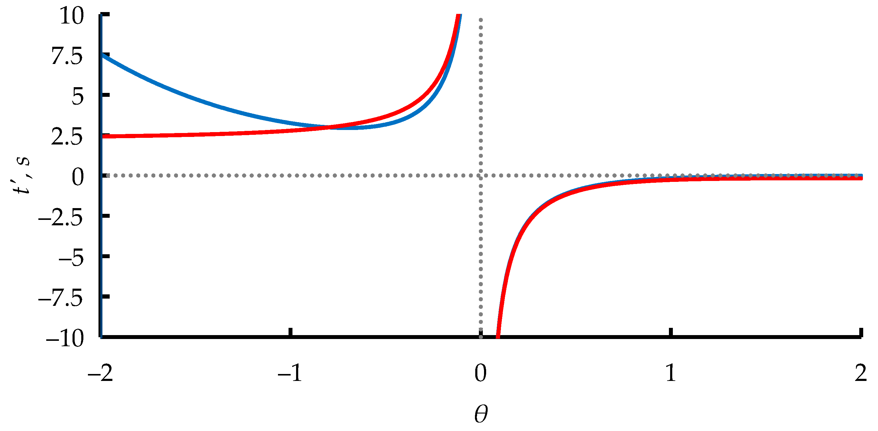
.
Figure 1 shows that for real and positive rapidity
, the graphs of the dependence of the spacetime interval and the local time coordinate
coincide in the direction.
Equation (15) for
s in the direction of the local time
is also easy to obtain from the geometric relations for
in the inertial frame
K and for
in the inertial frame
(e.g., see Reference [
11]), i.e.,
taking the proper coordinate
t from Equation (6) and assuming that the observer in inertial frame
chose
to be equal to zero.
Just as for the relation for
s in terms of the local time
, it is possible to introduce a perpendicular spacetime interval
in terms of the coordinate
. In Reference [
15], the following formula was obtained for the connection of the coordinates
and
from geometric considerations, where substituting in the proper coordinate
from Equation (6) gives
The derivatives of the Lorentz spacetime coordinates from Equation (11) with respect to
s are given by
and for
and
along the spacetime interval
, the following relations hold:
where
and
are the integrals of motion of a relativistic particle.
For
, taking the double derivative with respect to s from Equation (10) and assuming that the action is
give
From Equations (18)–(20), it is possible to represent the following local coordinates in forms:
i.e., the rotation operation is carried out, and the Lorentz spacetime coordinate
becomes purely a coordinate of the local time
for an observer in the inertial frame
, while
still contains components of space
q and time
t for an observer in the inertial frame
K.
Adding Equations (21) and (22) gives the local time coordinate
from Equation (10), and subtracting Equation (21) from Equation (22) gives
A similar case can be imagined when the observer in the inertial system
has one spatial coordinate
, while the observer in the inertial system
K has coordinates
t and
q, i.e.,
where adding Equations (24) and (25) gives the relation for the particle velocity from Equation (23). Subtracting Equation (24) from Equation (25) gives the coordinate
via Equation (10).
Differentiating Equations (21) and (22) with respect to
gives
where on the spacetime interval
s for
, the following hold:
Figure 2 shows a graph of Equations (20) and (27) as a function of the rapidity
.
As can be seen from
Figure 2, Equations (20) and (27) are satisfied only for real and positive
. In the present case, the inertial frame
is chosen relative to the position of the particle in such a way that
for
.
4. The Relationship between the Perpendicular Rapidity and the Angular Rapidity of a Free Relativistic Particle
Having projected the motion of a relativistic particle along the direction of one of the gyrovectors
or
, for the Hamiltonian
H, the following equations of motion hold and describe the components of the particle momentum from Equation (9):
where the angular rapidity
and the perpendicular rapidity
have the forms
The relationship between
and
is defined as
5. Expansion into Rapidity Spectra for the Lagrangian, Hamiltonian, and Momentum of a Free Relativistic Particle
The spectral–angular characteristics of a relativistic particle allow for the interpretation of the indefinite integrals of an arbitrary function
with respect to
,
, and
i.e.,
where the integrations allow
to be decomposed into spectra in terms of elementary functions. The integration constant is usually determined from the Cauchy problem.
For the Hamiltonian of a free relativistic particle, the expansions into rapidity spectra in terms of elementary functions have the following forms:
For the Lagrangian
of a free relativistic particle, expanding into rapidity spectra gives
Decomposing the longitudinal impulse from Equation (7) into spectral components
and
gives
Decomposing the transverse momentum
of the particle from Equation (9) into spectral components gives
Similarly, for the particle momentum
from Equation (9), the following hold:
6. Euler–Hamilton Equations in 3+1 Dimensions
For
,
, and
with respect to the invariant of the spacetime interval
ds from Equation (15), it is possible to introduce the following Euler–Hamilton equations describing the motion of a relativistic particle along the gyrovectors
,
, and
:
where
,
, and
are the coordinates describing the movement of the particle in the direction of the spacetime interval
s:
Regarding the “perpendicular” spacetime interval
from Equation (17), the Euler–Hamilton equations for
,
, and
have the forms
where
7. Decomposition of Local Coordinates into Rapidity Spectra
Some spectral decompositions have complex forms, such as
so it is convenient to introduce a so-called passage to the limit by analogy with relativistic hydrodynamics with coupled parameters [
23].
The simplest way to expand a coordinate
q into a spectrum in terms of
without using the explicit integral form of Equation (39) is to multiply and divide by
t in the integrand and then adopt the following transition:
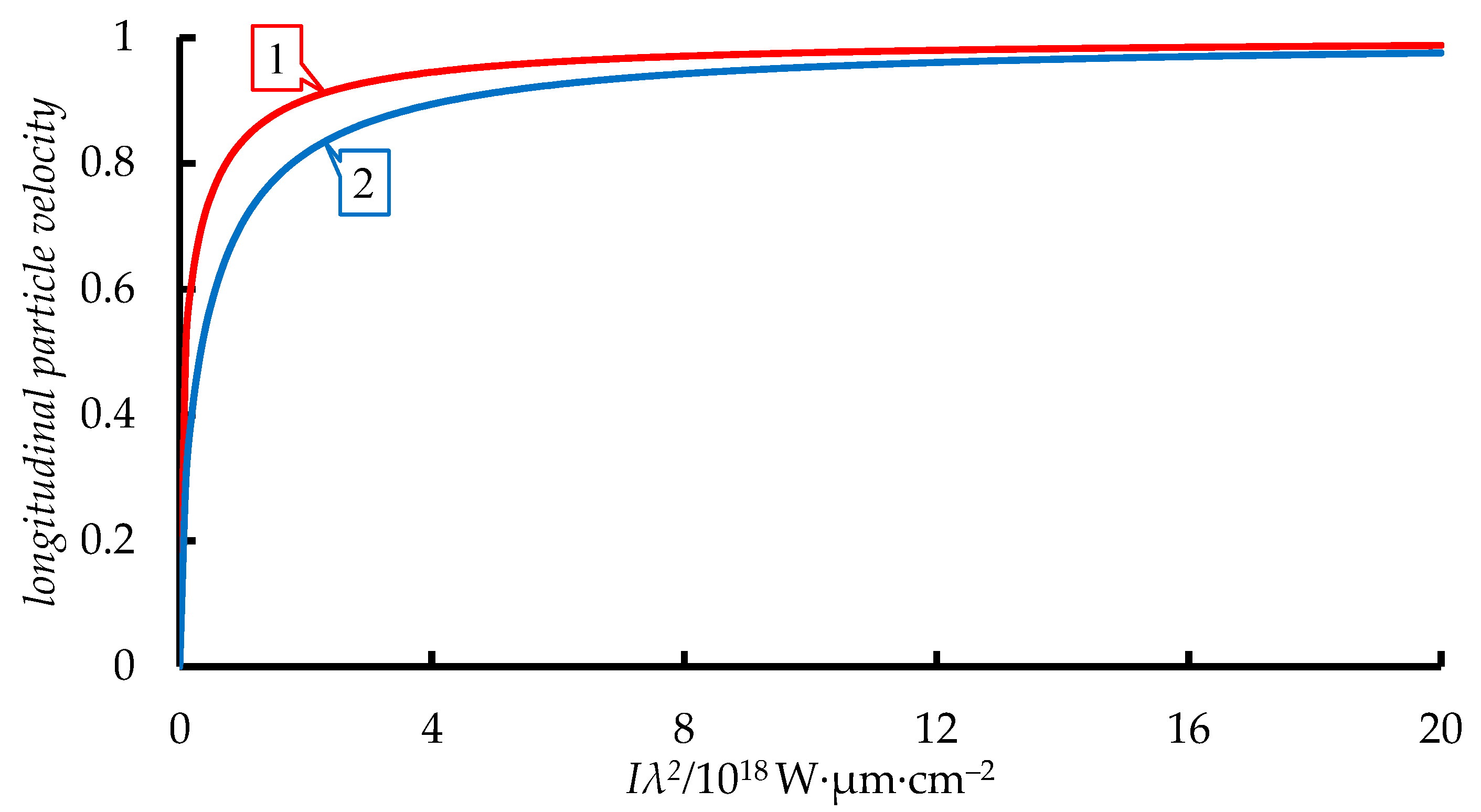
The passage to the limit is introduced by the arrow and is introduced because the relation for the coordinates
from Equation (6) goes into Equation (23) only for particle oscillations in a high-intensity field with
W·μkm·cm
−2 (see
Figure 3). Adopting the passage to the limit for the local coordinates from Equation (10) gives
Expanding the local coordinate
into rapidity spectra gives
where the integration constant is taken to be zero. Next, the obtained elementary functions
,
,
, and
form the basis for composing the Euler–Lagrange equations in 3+1 dimensions.
A scenario is now considered in which electrons are accelerated by the transverse electromagnetic field of incident pulsed laser radiation. The temperature of the fast electrons can be estimated as outlined in Reference [
29]. The amplitude of an oscillating electron should increase in the field of a linearly polarized electromagnetic plane wave. The expressions for the amplitude of the oscillating electron are substituted in
where
is the dimensionless amplitude,
is the electron charge,
is the electron mass,
c is the speed of light,
is the amplitude vector for the electric field of the incident electromagnetic wave,
is the polarization gyrovector,
is the oscillation frequency,
is the intensity of the incident linearly polarized electromagnetic wave (in W/cm
2), and
is the relativistic intensity:
where
is the wavelength (in
). The relation between the dimensionless momentum and the dimensionless field amplitude in Equation (46) is a function of the dimensionless intensity
. There are several possible equations for
that differ only by a constant. As in Reference [
30], the best criterion for such a determination can be identified by comparing the maximum total energy of an electron oscillating in the field of a laser pulse and its rest energy
mec2.
8. Spectral Characteristics of a Relativistic Particle in Field of a Circularly Polarized Electromagnetic Wave in 3+1 Dimensions
The movement of a relativistic charge in the field of a circularly polarized monochromatic electromagnetic wave is now considered. It is assumed that the plane wave and the relativistic particle are collinear to the direction of propagation of the normal gyrovector
. The four-vector potential of the wave then has the form in Reference [
28]:
where
E (a constant) is the wave amplitude,
ω (also a constant) is the oscillation frequency, and
and
are the orthogonal basis vectors relative to the normal gyrovector
.
The dimensionless Lagrangian of a relativistic particle in an external electromagnetic field, which depends on the rapidity
, has the following form [
28]:
Substituting (46) and (48) into (49) gives the Lagrangian describing the dynamics of a relativistic particle in the field of a plane monochromatic wave as a function of the rapidity:
Here, the dimensionless field amplitude for a plane wave is a constant ().
The rapidity of a particle in an electromagnetic field includes the rapidity of a free relativistic particle , i.e., . The electromagnetic rapidity can be written as , where is a small increment of the rapidity of the electromagnetic field. Due to the fact that conditions are imposed on and (the rapidities must be real, positive, and continuous), the speed of movement of a particle in an electromagnetic field and the speed of movement of a free relativistic particle are limited in the interval along the ordinate axis. Due to the small increment it can be further assumed that the rapidities are approximately equal, .
The connection between the Lagrangian and the Hamiltonian can be determined from the relationship between the integrals of motion of a relativistic particle that determine the longitudinal momentum of the particle. The relationship is valid for both a free relativistic particle and a relativistic particle in an external electromagnetic field:
where
is the integral of motion of a relativistic particle.
Substituting the Lagrangian from Equation (50) into Equation (51) gives the Hamiltonian of a particle in the external field of a plane monochromatic circularly polarized electromagnetic wave, i.e.,
where, if the particle has no velocity at the initial moment in time (i.e.,
), the Hamiltonian of Equation (52) has the form
.
Expanding the Lagrangian of Equation (50) into spectra in terms of
,
, and
gives
where the components of oscillation of a particle in a plane wave, which contain the dimensionless field amplitude
a, are added to the existing spectral components from Equation (34).
Adopting the passage to the limit
for the Hamiltonian of Equation (52) and expanding into spectra in terms of
,
, and
gives
where
is a polylogarithmic function [
31].
From the solutions of Equations (53)–(57), the expansions of the Hamiltonian and Lagrangian of a particle in the field of a plane wave are non-trivial solutions for the related parameters, which allow estimation of the rapidity-dependent spectral components of the motion of a relativistic particle for a constant field amplitude a. Next, it is shown that spectral decomposition of the motion of a relativistic particle in the field of a plane wave with a constant field amplitude is more complex than that in the case of a plane laser pulse with a rapidity-dependent dynamically varying amplitude.
9. Spectral Characteristics of Relativistic Charge in the Field of a Plane Laser Pulse in 3+1 Dimensions
To describe the dynamics of a relativistic particle in the field of a plane laser pulse, it is assumed that the dimensionless field amplitude in the Lagrangian from Equation (50) is not constant, and the value of the field amplitude changes in accordance with Equation (44). Then, the Lagrangian describing the dynamics of a charged particle in the field of a plane laser pulse with right-handed circular polarization, which depends on
, has the form
Substituting the Lagrangian from Equation (58) into Equation (51) gives the Hamiltonian of a particle in the field of a right-handed circularly polarized electromagnetic wave, i.e.,
Expanding the Lagrangian of a particle with right-handed circular polarization from Equation (58) into spectra in terms of
,
, and
gives the following spectral representations:
Similarly, for the Hamiltonian of Equation (59), expanding into rapidity spectra gives
For a particle in the field of a plane laser pulse with left-handed circular polarization, the Lagrangian representation is
and from Equations (64) and (51), the Hamiltonian of the system in the field of a plane circularly polarized laser pulse is
Expanding Equations (64) and (65) into rapidity spectra gives
Adding the spectral characteristics of the radiation of a relativistic charge in the field of a plane laser pulse with right and left circular polarizations and considering the normalization factor gives the spectral characteristics of the radiation for a free relativistic particle, as in Equations (33) and (34). As can be seen from the presented solutions, the spectral components of a relativistic particle in the field of a plane wave and a laser pulse using transformation from Equation (5) in the Euclidean phase plane are described well by the expansion in rapidity in the direction of the polarization gyrovector , because in all cases it has a real oscillatory part.
10. Dynamics of a Relativistic Particle in the Field of a Plane Laser Pulse with Left-Handed Circular Polarization in 3+1 Dimensions
To describe the dynamics of a relativistic particle in the field of a plane circularly polarized laser pulse along the spacetime interval
s, it is convenient to use
and replacing the Lagrangian of a particle in the field of a left-handed circularly polarized laser pulse with that of a right-handed one gives the following oscillating parameter:
Because the spacetime interval s from Equation (15) contains the Gudermannian function and the derivative of the perpendicular spacetime interval with respect to , it is of further interest to introduce the Euler–Lagrange equation, which depends only on the Gudermann function or the perpendicular spacetime interval .
Regarding the angular rapidity
, it is also convenient to introduce the following Euler–Lagrange equation for a left-handed circularly polarized wave:
where
L is the Lagrangian of a free relativistic particle. Similarly, substituting
into Equation (72) gives the following oscillatory parameter:
Regarding the perpendicular rapidity
, for a particle in the field of a plane left-handed circularly polarized laser pulse, the following equation holds:
where substituting in
gives the following oscillatory parameter:
Regarding the perpendicular spacetime interval
and the rapidities
,
, and
, the following Euler–Lagrange equations of motion hold in the field of a plane laser pulse with left-handed circular polarization:
where
and
.
Thus, in 3+1 dimensions, the dynamics of a relativistic particle are described well by the Euler–Lagrange equations using , , and , both in the direction of motion and in the field of a circularly polarized laser pulse. As can be seen, from the rapidities , , and given here instead of the spacetime interval , the resulting solutions are compact, and for a particle in the field of a left-handed circularly polarized wave, they allow coordinates to be obtained that describe the dynamics of the particle in 3+1 dimensions. The introduced coordinates relative to the dynamics of a particle in the field of a left-handed circularly polarized laser pulse are also valid for a right-handed circularly polarized pulse, but the equations have a dissipative oscillation parameter depending on the selected rapidities and spacetime intervals.
11. New Lorentz-Invariant Transformations in 1+1 and 3+1 Dimensions
The sum of the coordinates q,
, and
from Equations (6) and (8) in 3+1 dimensions relative to the derivative with respect to the rapidity
has the following form:
The spectral decomposition of the longitudinal component of the particle’s momentum in terms of and gives the coordinate and the rapidity (see Equation (35)) along the normal gyrovector .
Equations (35) and (77) lead easily to a new representation of the Lorentz spacetime coordinate
as
where
. Differentiating Equation (78) with respect to
gives a connection between the Lorentz spacetime coordinates
,
and the integral of motion of a relativistic particle
as follows:
As can be seen from Equation (79), when describing the dynamics of a particle using the new Lorentz spacetime coordinate
, when passing from
to
, it is necessary to make the following replacement of coordinates and operators:
For example, from Equation (80), the classical equation of particle motion in an electromagnetic field can be represented in the form
where
is the momentum of the particle in the electromagnetic field,
is the speed of movement of the particle in the electromagnetic field, and
and
are the intensities of the electric and magnetic fields, respectively, depending on the new Lorentz spacetime coordinate.
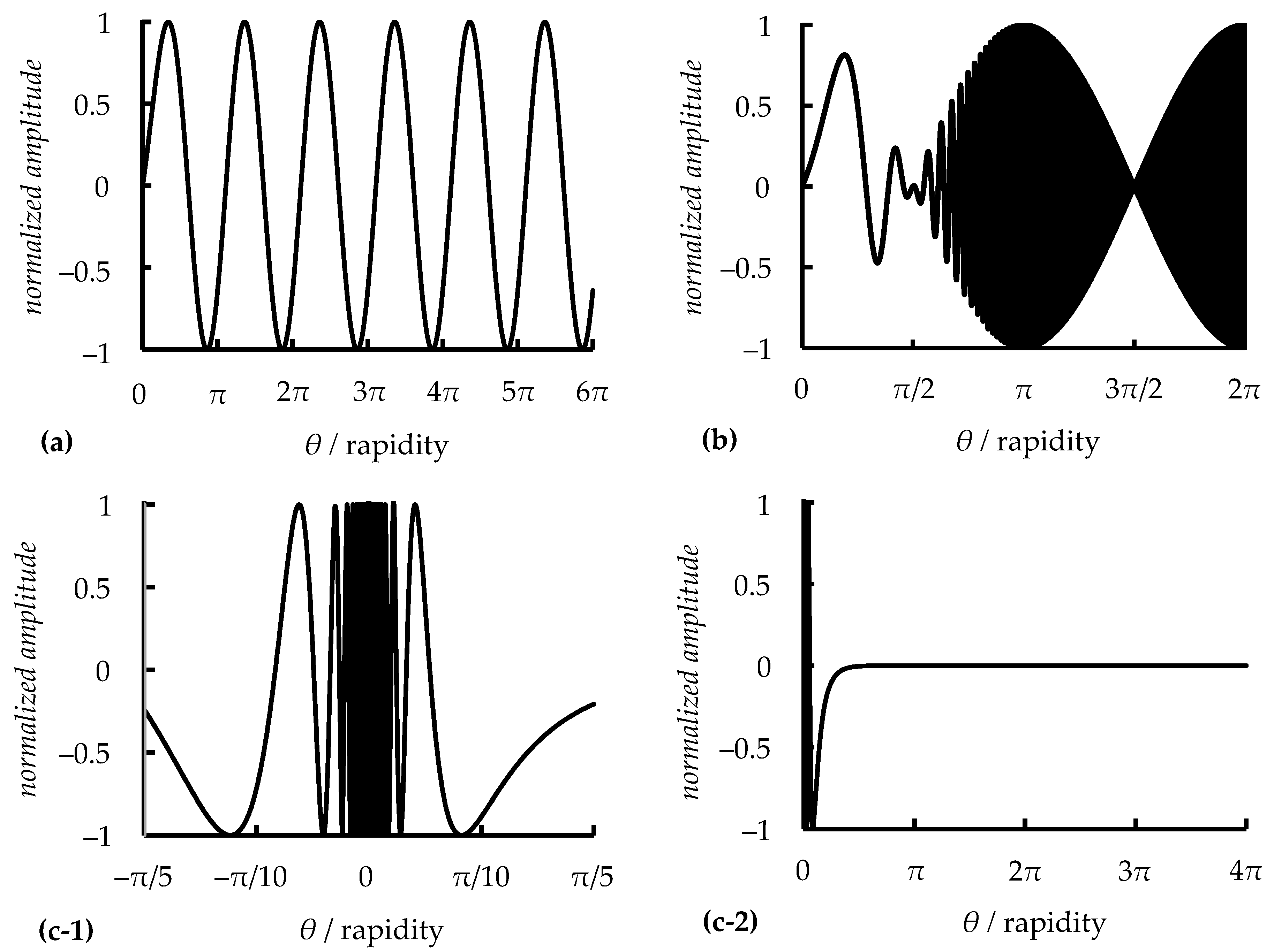
The advantage of using the new Lorentz spacetime coordinate with coupled parameters
for plane electromagnetic waves with constant field amplitude as in Equation (48) is that the representation
describes the periodic motion of a charge in the field of a plane monochromatic electromagnetic wave for real and positive
(see
Figure 4a). It is also advantageous to use the new Lorentz spacetime coordinate
to describe the dynamics of a particle in a constant uniform field when the oscillation frequency of the particle does not change and
. If the oscillation frequency of a particle changes according to a harmonic law
(see Reference [
32]), then with an increase in
, frequency modulation is observed in the field of a plane wave (see
Figure 4b). Thus, the Lorentz spacetime coordinate
is the simplest representation for describing the dynamics of a relativistic particle with coupled parameters.
Using the Lorentz spacetime coordinate
to describe the dynamics of a particle in the field of a plane laser pulse,
Figure 4(c-1,c-2) shows that
describes a modulated pulse over the interval
, where the oscillation frequency is considered constant
.
If it is also imagined that the oscillation frequency of a particle changes according to a harmonic law
(see Reference [
32]), then in this case, the wave oscillation profile does not change and has the same values as for a constant frequency (see
Figure 4(c-1,c-2)). Here, it can be seen that
describes the dynamics of a particle in a wave with spatial modulation.
Applying the Lorentz transformations for
from Equation (78) gives the coordinates
and differentiating Equation (82) with respect to
gives
Equations (6), (8), (10) and (82) give a connection between the coordinates in the inertial systems
K and
in 3+1 dimensions via
, i.e., the general system of equations can be written in the following form:
where the connection between the angular coordinates
and
in the inertial systems K and
is also determined via the rapidity
from Equation (82), i.e.,
As well as the existing Lorentz spacetime coordinate
from Equation (78), it is possible to introduce an additional coordinate of the form
and applying the Lorentz transformations for
from Equation (86) gives
Differentiating Equation (87) with respect to
gives
and it can be seen that the projection of the motion of a relativistic particle is relative to
and
chosen along the perpendicular spacetime interval
.
The obtained correct coordinates
and
also give another angular Lorentz spacetime coordinate,
where the application of the Lorentz transformation to the coordinate Equation (85) yields the following local coordinates in the inertial system
:
Differentiating Equation (90) with respect to
gives
The local rapidities
,
,
, and
form Lorentz spacetime coordinates in 3+1 dimensions, where the generalized system of equations for
has the form
Here, the Lorentz spacetime coordinates
,
, and
are obtained with respect to the Lorentz transformation, and differentiating them gives the derivatives of spacetime intervals
,
, and
from Equations (83), (88) and (91). This result can also be obtained by the method of calculus of variations, similar to Reference [
26], only that here it is necessary to apply the replacements given in Equation (80), where the following correspondences hold:
From Equations (83), (88) and (91), it is clear that the actions are described by the functions , and , which are hyperbolic functions that depend on only .
12. Descriptions of the Kinetic Energy of a Relativistic Particle in 3+1 Dimensions in the Field of a Flat Circularly Polarized Laser Pulse Using the “New” and “Old” Lorentz Spacetime Coordinates
The advantage of the method of coupled parameters in 3+1 dimensions is that there is no need for the analysis to introduce initial conditions describing the motion of a relativistic particle, since all parameters depend on one parameter, for example, the rapidity . Therefore, physical processes can be considered in the dynamics without considering the initial conditions.
As is well known, the components of the transverse momentum of a particle in the field of a plane circularly polarized laser pulse as in Equation (48) in 3+1 dimensions have the form
where the energy and longitudinal component of the momentum of the particle are determined through the integral of motion of the relativistic particle
,
As can be seen from Equation (96), in the absence of transverse momentum of the particle , the formulas transform to describe the dynamics of a free relativistic particle in 1+1 dimensions.
For example, if the Cauchy problem is adopted to analyze the energy of a particle from Equation (96), similarly to in works [
33,
34,
35], it is assumed that at the initial moment of time
, the particle has a zero coordinate
, and the speed of the particle is equal to zero
.
Since the particle speed has a connection with the integrals of motion in Equation (19), at the initial time, the rapidity is
. Then, the kinetic energy of the particle from Equation (96), similarly to in Reference [
36], has the following connection with the longitudinal and transverse components of the particle momentum in the field of a plane circularly polarized laser pulse (or in the field of a plane wave), where relativistic corrections are not taken into account, and the formula takes the form of classical kinetic energy in the non-relativistic case:
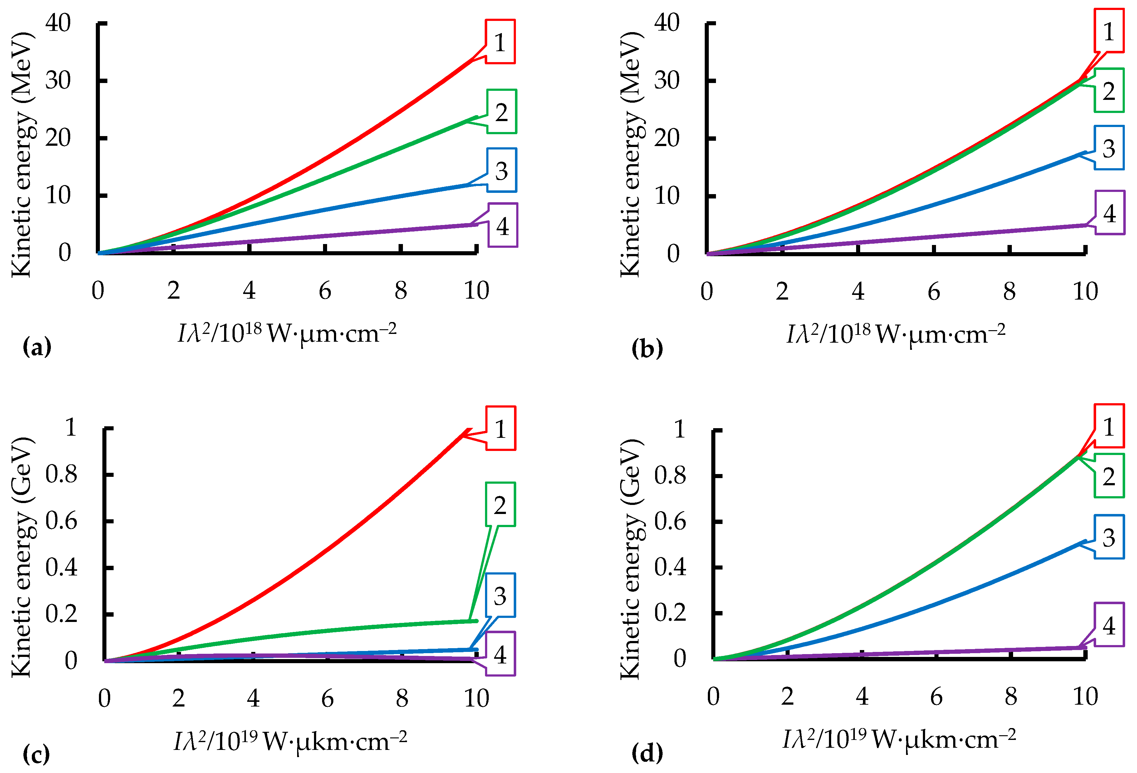
Figure 5 shows graphs of the dependence of the kinetic energies of the particle in Equations (96) and (97) on the dimensionless field amplitude
a. In Equation (96), the coupled parameters described by Equation (46) are expressed in terms of the dimensionless field amplitude
a.
For an oscillating particle, representations of the “old” and “new” Lorentz spacetime coordinates in the field of a plane laser pulse are presented. That is, it is assumed that the particles oscillate in the field of a laser pulse, in which the coordinates for the “old” , , and “new” , , Lorentz spacetime forms are initially specified.
As can be seen from
Figure 5, the Lorentz spacetime coordinates
and
represent a fairly close oscillation energy of the particle. For a laser field intensity
W·cm
−2, the kinetic energy of the electron is on the order of 0.9–1 GeV. From
Figure 5b, it is clear that for a laser field intensity
W·cm
−2, the “new” Lorentz spacetime coordinates
and
are equal, and for a laser field intensity
W·cm
−2, they are 30 MeV.
It can also be seen from
Figure 5 that Equation (97) automatically describes the kinetic energy of a particle in the field of a laser pulse in the non-relativistic case. In an intense laser field
W·cm
−2, the Lorentz spacetime coordinates
and
describe the value of the kinetic energy of a particle close to the non-relativistic case, where the kinetic energy is approximately
0.2 GeV and
9.5 MeV. For the “new” Lorentz-invariant coordinate
, the particle energy value also corresponding to the relativistic oscillation limit for the laser field intensity
W·cm
−2 is
0.5 GeV.
From the “old” and “new” Lorentz spacetime coordinates and , it is clear that in the intensity range W·cm−2, there is a transition of particle oscillations from the MeV range to the GeV range of particle energy.
13. Comparison of the “New” and “Old” Lorentz-Invariant Coordinates with Fermi Coordinates
The Fermi eigen coordinates have the following form [
37]:
where
is the particle’s proper acceleration,
is the proper time, and
s is a spacetime interval. In the Fermi representation, a spacetime interval
s is selected according to the direction of the coordinate
, that is, in Equation (98),
.
To compare the obtained “new” and “old” Lorentz spacetime coordinates with the Fermi coordinates under the acceleration of a relativistic particle, the proper acceleration can be written as
Similarly, for the Fermi coordinates (98), it is possible to introduce the following representation:
where
.
Since the Fermi coordinates are metric representations from the general theory of relativity and are generalized to the case of pseudo-Riemannian spaces [
37], and the resulting “new” and “old” Lorentz spacetime coordinates are representations from the special theory of relativity in the representation of Lobachevsky geometry, to compare them, it is necessary to introduce a common parameter that would be the same in both cases. Here, it is proposed that the optimal parameter for comparing the available coordinates is the rapidity
, since the rapidity is a monotonically increasing function that tends to infinity when the particle speed approaches the speed of light.
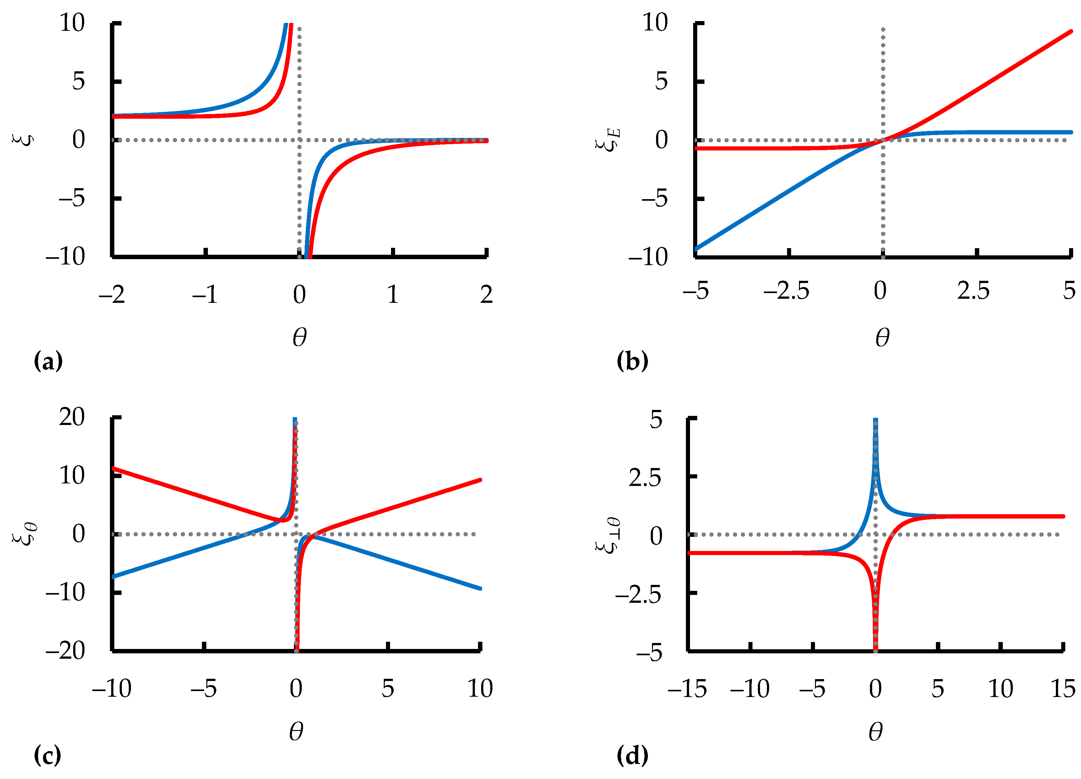
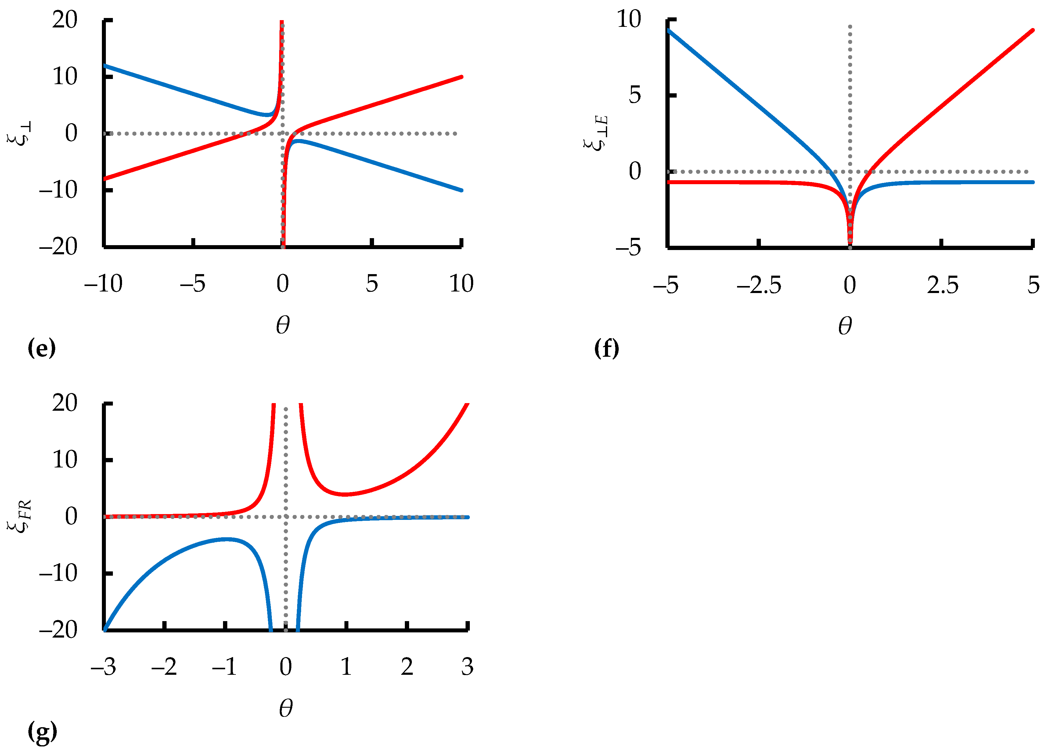
Figure 1 shows a graph of the dependence of the “old” (Equations (6) and (8)) and “new” (Equations (78), (86) and (89)) Lorentz spacetime coordinates and the Fermi spacetime coordinate (100) on the rapidity
.
The next step is to analyze the Lorentz spacetime coordinates and Fermi coordinates depending on the real and positive rapidity
. As can be seen from
Figure 6, for the coordinates
,
,
,
,
, and
, the relativistic motion of the particle for
is defined by functions bounded from above:
,
,
,
, and
.
For coordinates
,
, the functional dependence on the rapidity
for
is increasing. For coordinates
,
, on the contrary, the functional dependence on the rapidity
for
is decreasing, as seen in
Figure 6c,e.
From
Figure 6b,f, it can be seen that for
, the coordinates
and
are bounded from above by
and
. For
, the functional dependences
and
are increasing.
Figure 6d shows that the advantage of the coordinates
and
is that in the interval
, the coordinates have a limitation for the value along the ordinate axis, the coordinate
is bounded from above, and the coordinate
is bounded from below.
As can be seen, the coordinate and the Fermi coordinate in the fourth coordinate quaternary for have the same physical values, where the particle velocity changes in the next interval .
The coordinate and the Fermi coordinate , also in the fourth coordinate quarter for , have the same physical values, where the particle velocity changes in the next interval .
Thus, clearly, the coordinate and the Fermi coordinate have the same physical values in the sub-relativistic, relativistic, and ultra-relativistic regions for a field intensity W·cm−2. The coordinates and have the same physical values in the relativistic and ultra-relativistic regions for the field intensity W·cm−2.
14. Comparisons of the Proper Lorentz Groups SO(1,3) with Coupled Parameters
This section presents representations of the proper Lorentz groups SO(1,3) for coupled parameters depending on the rapidity
for “old” and “new” Lorentz coordinates. By definition, the proper Lorentz group retains a quadratic form:
where
,
,
,
are proper metric coordinates.
Associating the metric coordinates
,
,
,
results in the following representations of the proper Lorentz group
depending on the rapidity
expressed in terms of the “old” Lorentz coordinates:
Similarly, introducing a change for the new Lorentz coordinates
,
,
,
gives the proper Lorentz group
:
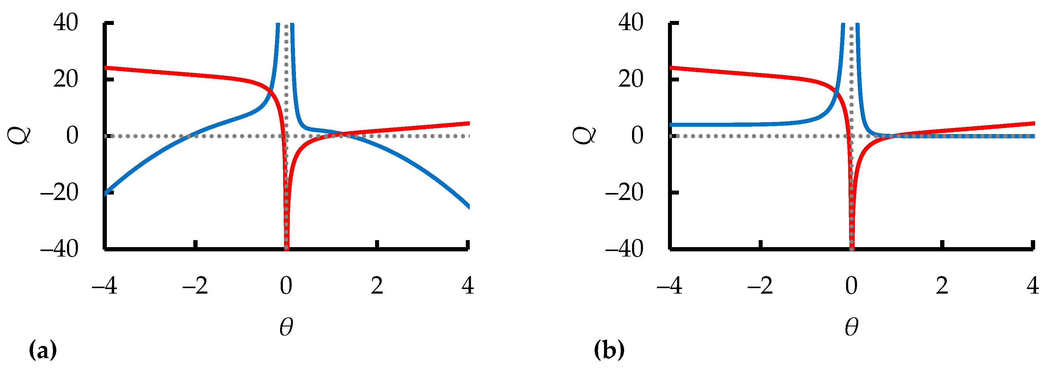
As can be seen from Equation (102) and
Figure 7a for the proper Lorentz group SO(1,3) for
at
, the eigenvalues of the coordinates have the form
,
,
, and
. As
, the particle speed tends to
of the speed of light, and the real parts of the proper coordinates in Equation (102) tend to
,
, and
. As
, the speed of the particle tends to the speed of light
, and the real parts of the coordinates in Equation (102) tend to
,
,
, and
.
For the proper Lorentz group SO(1,3) for as , the eigenvalues of the coordinates tend to , , and . When tends to , the eigenvalues of the coordinates tend to , , and . As tends to , the eigen coordinates take the form , , and .
Figure 7 shows that for real and positive
, for the proper Lorentz group SO(1,3) for
in the interval
, the functional dependence
is decreasing. For
in the interval
, the functional dependence
is increasing.
As seen from
Figure 7b, in 1+1 dimensions, the functional
dependence on
in the interval
is bounded from below and tends to
.
Thus, if it is necessary to describe the motion of a relativistic particle for an increasing or decreasing function in an interval , it is convenient to apply the proper Lorentz group SO(1,3) for or . To describe the motion of a relativistic particle in the interval along zero with respect to the rapidity , it is convenient to adopt the spacetime interval in 1+1 dimensions when .
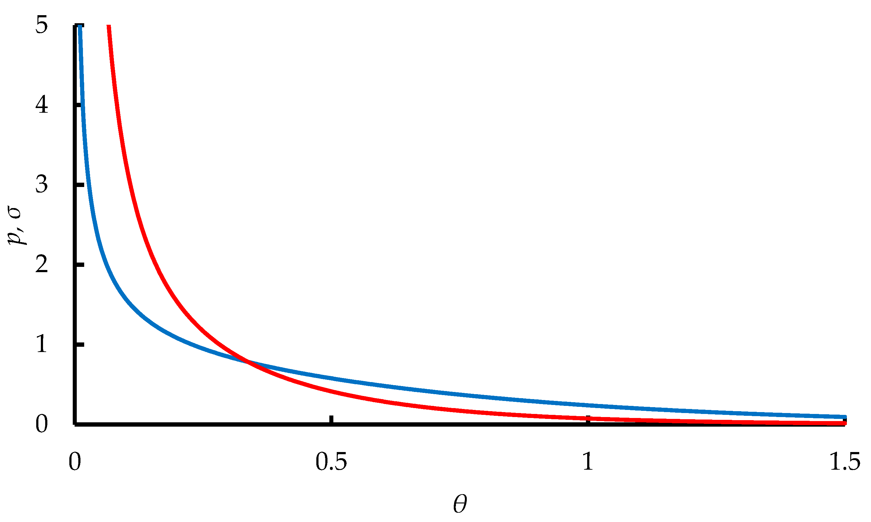
15. Relationship between the Pressure and Energy Density in Relativistic Hydrodynamics with Coupled Parameters in 1+1 Dimensions
In this section, isotherms of the pressure and energy density of a relativistic particle are obtained as a function of the rapidity . The development of a relativistic approach to hydrodynamics is of great interest because there is no need to work with the microscopic properties of individual nucleons or ions, but it is necessary to work with certain macroscopic parameters of the system such as the pressure and energy density.
The stress–energy tensor of relativistic hydrodynamics has the following form in four dimensions following Reference [
38]:
where
is the thermal function of a unit volume,
is the pressure,
is the energy per unit volume,
is the four-dimensional speed, and
is a metric tensor with components of the form
,
for
. Furthermore, the thermodynamic quantities
and
are understood as taking their eigenvalues per unit volume in the local field system.
In Equation (104), the following notation is also used in 1+1 dimensions:
where
is the Lorentz spacetime coordinate and
,
,
.
The components of the stress–energy tensor from (104) in 1+1 dimensions, depending on the rapidity
, have the dependence
The relativistic hydrodynamic equation of motion in four dimensions has the following form:
and in 1+1 dimensions:
As is well known, when considering hydrodynamics, it is necessary to have an equation of state for the matter of the system. As an equation of state for the ideal matter of the system for energy
, as a rule, the following functional relationship between the pressure
and energy density
is used [
38]:
As stated in Reference [
39], there is at present no rigorous evidence for the relationship between the density of matter
and pressure
in the ultrarelativistic case (Equation (109)), but according to Landau, the assumption above is highly plausible.
In this section, for the equation of motion of an ultrarelativistic fluid (Equation (108)), the problem will be solved in 1+1 dimensions with coupled parameters and . A more rigorous definition of and through the rapidity is now introduced, and it is shown that for the equation of state of an ideal substance, the connection in Equation (109) is universal and plausible for related parameters.
Substituting Equation (106) in Equation (108) gives the following differential equations:
the solution of which is
where
and
are constants.
The constants
and
are selected in such a way that the terms of thermal radiation have the closest value in relation to each other, with the functional dependence in Equation (109) for
satisfied (
Figure 8).
Finding an exact analytical solution for the various thermodynamic characteristics of radiation is a rather difficult task. Therefore, for
and
, the first approximation in the expansion of the Taylor series in the vicinity of
is adopted here, giving
that is, the more general relationship between the pressure and energy density is
16. Conclusions
In this work, the form of the local coordinates and local rapidities in 3+1 dimensions was obtained via parametrization with coupled parameters. New Lorentz spacetime coordinates were presented (Equations (78), (86) and (89)) that make it possible to describe the dynamics of a particle in 3+1 dimensions with coupled parameters in terms of hyperbolic functions depending on the rapidity
. The resulting “new” Lorentz spacetime coordinates are an addition to the “old” Lorentz spacetime coordinates (Equations (6) and (8)), which together describe the dynamics of a particle in 3+1 dimensions. As shown in this article, the solutions are valid only for real and positive rapidities
(
Figure 1 and
Figure 2, Equations (10), (15), (20) and (27)).
For the dimensionless amplitude of a field
W·μm·cm
−2, the velocities of particle motion
and
become equal (
Figure 3), and as a result, it is possible to introduce a passage to the limit (Equation (43)).
A perpendicular rapidity and an angular rapidity (Equation (30)) were derived from Hamilton’s formalism; these are not invariant, but in combination with other rapidities, they form new Lorentz spacetime coordinates (Equations (86) and (89)) with respect to Lorentz transformations relative to the intervals and .
Because all the parameters are coupled, it was shown that an arbitrary function can be decomposed via the rapidity into elementary functions. For those cases in which it is not possible to decompose an arbitrary function into elementary ones, a so-called passage to the limit was introduced (Equation (43)), which allows a complex function to be decomposed into elementary functions using the rapidities , , and .
The spectral expansions into elementary functions resulted in the coordinates , , and (Equations (78), (86) and (89)), and a comparison between the Lorentz spacetime coordinates and was carried out through the integral of motion of a relativistic particle (Equation (79)).
It was shown that for plane waves oscillating according to a harmonic law, the Lorentz spacetime coordinate
describes the oscillation of a particle over an interval
, similar to the oscillation of a particle in the field of a short laser pulse. Applying the new Lorentz spacetime coordinate
to plane waves oscillating according to the harmonic law, it is clear that the oscillation of a particle in a wave is described by periodic motion in the interval
(
Figure 4).
Assuming that the plane waves have frequency modulation, with the frequency varying according to the harmonic law
and
, for a plane wave described by the Lorentz spacetime coordinate
, the presence of frequency modulation does not affect the oscillation frequency of the particle because
describes the dynamics of the particle with spatial modulation. When applying the frequency modulation
to the new Lorentz spacetime coordinate
, the wave form clearly has a classical frequency-modulated profile. From the Lorentz spacetime coordinates
and
in relation to plane waves, the main conclusion that can be drawn is that (i) the use of
describes the dynamics of a particle in short pulses well, and (ii) the use of the new Lorentz spacetime coordinate
describes classical harmonic processes (
Figure 4).
In general, it was shown that the Euler–Hamilton equations (Equations (38) and (40)) describe the dynamics of a relativistic particle well in the field of a plane wave and in the field of a plane laser pulse in 3+1 dimensions. It was also shown that to describe the motion of a particle in the field of a circularly polarized pulse with left-hand polarization, it is advantageous to use the Euler–Lagrange equations (Equations (70)–(76)) because the resulting equations are compact.
When comparing the descriptions of oscillations of the kinetic energy of a particle in the field of a plane laser pulse using the “old” and “new” Lorentz spacetime coordinates, it was shown that the particle has maximum kinetic energy when using coordinates
and
, the values of which are approximately equal throughout the spectral range (
Figure 5).
Furthermore, when comparing the “new” and “old” Lorentz spacetime coordinates with the Fermi coordinates, it was shown that the spacetime coordinates
and
have a general solution for the rapidity
(
Figure 6a,g).
For the proper Lorentz group SO(1,3) with coupled parameters, it was shown that to describe the motion of a relativistic particle for an increasing or decreasing function in an interval
, the proper Lorentz groups
or
are convenient (
Figure 7).
As an example of the applicability of coupled parameters, a more general relationship was also demonstrated between the pressure and energy density expressed through isotherms as a function of the rapidity
in relativistic hydrodynamics with coupled parameters in 1+1 dimensions (
Figure 8). The results of this work will be used in the future to construct a relativistic hydrodynamic model with coupled parameters in 3+1 dimensions.


 ,
, 
