Single-Shot Factorization Approach to Bound States in Quantum Mechanics

Abstract

Using a flexible form for ladder operators that incorporates confluent hypergeometric functions, we show how one can determine all of the discrete energy eigenvalues and eigenvectors of the time-independent Schrödinger equation via a single factorization step and the satisfaction of boundary (or normalizability) conditions. This approach determines the bound states of all exactly solvable problems whose wavefunctions can be expressed in terms of confluent hypergeometric functions. It is an alternative that shares aspects of the conventional differential equation approach and Schrödinger’s factorization method, but is different from both. We also explain how this approach relates to Natanzon’s treatment of the same problem and illustrate how to numerically determine nontrivial potentials that can be solved this way.

1. Introduction

The goal of this work was to solve the energy eigenvalue equation in single-particle quantum mechanics (often called the time-independent Schrödinger equation). This is usually formulated in position space, where, for example, in one dimension, the momentum operator is represented by $\widehat{p}=-i\hslash d/dx$, and the time-independent Schrödinger equation becomes the second-order linear differential equation

$$-\frac{{\hslash }^2}{2M}\frac{d^2}{d{x}^2}\psi \left(x\right)+V\left(x\right)\psi \left(x\right)=E\psi \left(x\right),$$

(1)

for the energy eigenvalue E and the energy eigenstate, which is represented as a wavefunction $\psi \left(x\right)$. Here, $V\left(x\right)$ is the potential that the particle moves in and M is the particle’s mass. This equation was introduced by Schrödinger in 1926 [1].

Fourteen years later, Schrödinger developed another approach to solve for energy eigenvalues and eigenstates [2]. It uses a representation-independent methodology that factorizes the Hamiltonian in the form

$$\widehat{H}=\frac{{\widehat{p}}^2}{2M}+V\left(\widehat{x}\right)={\widehat{A}}^{†}\widehat{A}+E\mathbb{I}.$$

(2)

Here, $\widehat{x}$ and $\widehat{p}$ are operators that satisfy the canonical commutation relation $[\widehat{x},\widehat{p}]=i\hslash$, ${\widehat{A}}^{†}$ and $\widehat{A}$ are raising and lowering operators (also called ladder operators), and the factorization method determines the ground-state energy E without explicitly determining the ground-state wavefunction. Instead, it simply postulates the existence of a state that is annihilated by $\widehat{A}$ via the subsidiary condition $\widehat{A}|\psi \rangle =0$, and then, because the Hamiltonian is written as a positive semidefinite operator plus a constant, the energy of this state is given by E. The lowering operator is written as

$$\widehat{A}=\frac{1}{\sqrt{2M}}\left(\widehat{p}-i\hslash W\left(\widehat{x}\right)\right),$$

(3)

with W being the superpotential. Often, there are multiple choices for the superpotential that provide a factorization—one must choose the superpotential that satisfies some additional conditions that guarantee the ground-state wavefunction will be normalizable in order to have a valid solution. For example, in a one-dimensional problem, we need $W\left(x\right)$ to be positive for $x\to \infty$ and negative for $x\to -\infty$, and to be finite for all x (there can be additional conditions). When the superpotential satisfies these conditions, it is a supersymmetric superpotential. To find the higher energy eigenstates, one forms the factorization chain, which involves defining new auxiliary Hamiltonians, factorizing them, and constructing the higher-energy eigenstates by applying the appropriate ladder operators to each auxiliary Hamiltonian ground state. It would take us too far afield to describe the further details of that construction here, but this context provides the jumping off point for our work.

The name superpotential comes from a revival of the factorization method by Witten [3] in the 1980s, which led to the field of supersymmetric quantum mechanics. Supersymmetric quantum mechanics works with a single factorization, which is subsequently used to construct two partner potentials that are related to each other as two adjacent links in a factorization chain. The system of two Hamiltonians can be formulated into an additional two-by-two matrix structure that represents bosonic and fermionic sectors. Broken supersymmetry can be examined within this context as well. We will not discuss supersymmetric quantum mechanics further here, but we do note two books that provide further context for the method [4,5]. The problem of determining exactly solvable potentials within supersymmetric quantum mechanics has been studied widely. We mention in particular work led by Lévai, which is closely related in its approach to the work we present here [6,7,8]. While that work is focused on finding and clarifying different classes of exactly solvable potentials, our work here is focused on describing a different methodology for determining energy eigenstates.

Determining the initial factorization for the ground state typically requires the solution of a nonlinear Ricatti equation. Conversely, the ground-state wavefunction can always be employed to construct a factorization if it is known. We simply choose the superpotential to satisfy $W\left(\widehat{x}\right)=-{\psi }^{\prime }\left(\widehat{x}\right)/\psi \left(\widehat{x}\right)$, where the prime indicates a derivative with respect to the argument of the function; then, the Schrödinger equation is equivalent to the Ricatti equation for the superpotential:

$$\frac{{\hslash }^2}{2M}\left(-W^{\prime }\left(\widehat{x}\right)+W^2\left(\widehat{x}\right)\right)=V\left(\widehat{x}\right)-E\mathbb{I}.$$

(4)

In analytically solvable problems (so-called shape-invariant potentials), one can directly determine the superpotential without requiring an explicit solution of the Ricatti equation or knowing the ground-state wavefunction (an example is the well-known abstract operator method applied to the simple harmonic oscillator). Such cases are exceptions, not the general rule. Once one formulates the Ricatti equation, it can also be solved directly without a priori knowledge of the ground-state wavefunction to factorize the Hamiltonian.

The single-shot method for bound states is half-way between the Schrödinger equation and the factorization method. It works by finding a single factorization in a general form and then determines all of the allowed energies that yield normalizable solutions. This methodology has already been employed to find continuum eigenstates of exactly solvable problems [9]. The bound-state problems bring in a number of additional subtleties due to the quantization of the energy eigenvalues.

In this work, we develop the single-shot factorization method for bound states. We apply it to solve for all exactly solvable energy eigenvalue problems that can be solved with wavefunctions that include a confluent hypergeometric function multiplied by simple functions (powers, exponentials, Gaussians, etc.). This is the same problem that Natanzon solved [10], where he described all potentials that have confluent hypergeometric functions as part of their wavefunctions. Our approach is markedly different from Natanzon’s though, and we show in detail how the two methods interrelate.

2. Formalism of Single-Shot Factorization

In our general description, we examine problems in one-, two-, and three-dimensions. Rather than using $\widehat{x}$ for our general variable, we use $\widehat{q}$. It can represent the one-dimensional x, the two-dimensional radial coordinate $\rho =\sqrt{x^2+y^2}$, or the three-dimensional radial coordinate $r=\sqrt{x^2+y^2+z^2}$. The effective Hamiltonian of a system with a non-relativistic particle of mass M moving in an effective potential $V_{\mathrm{eff}}\left(\widehat{q}\right)$ then becomes

$$\widehat{H}=\frac{{\widehat{p}}_q^2}{2M}+V_{\mathrm{eff}}\left(\widehat{q}\right),$$

(5)

where $\widehat{q}$ represents the aforementioned radial coordinate operator and $V_{\mathrm{eff}}\left(\widehat{q}\right)$ is the “radial” potential that is derived using separation of variables. We use a subscript q on the momentum operator because in two or three dimensions, it will be the corresponding radial momentum operator.

We want to factorize the Hamiltonian in the form

$$\widehat{H}={\widehat{A}}_k^{†}{\widehat{A}}_k^{\phantom{†}}+E_k\widehat{I}$$

(6)

where $E_k$ is the energy of the system and ${\widehat{A}}_k^{\phantom{†}}$, which is the lowering operator, is given by

$${\widehat{A}}_k^{\phantom{†}}=\frac{1}{\sqrt{2M}}\left[{\widehat{p}}_q-i\hslash k{W}_k\left(k\widehat{q}\right)\right],$$

(7)

in terms of $W_k$, which is the superpotential, and k, which is a wavenumber that makes the superpotential and its argument dimensionless. We slightly changed the form of the superpotential here by introducing some constants that make the remainder of the analysis clearer. We hope this causes no confusion to the reader.

By using the subsidiary condition

$${\widehat{A}}_k^{\phantom{†}}|\psi \rangle =0,$$

(8)

we can express the superpotential in terms of a function $\psi \left(\widehat{q}\right)$:

$$W_k\left(k\widehat{q}\right)=-\frac{1}{k}\frac{d\psi \left(\widehat{q}\right)}{d\widehat{q}}\frac{1}{\psi \left(\widehat{q}\right)}=-\frac{1}{k}\frac{d}{d\widehat{q}}\left[ln\left(\psi \left(\widehat{q}\right)\right)\right].$$

(9)

The derivatives can be thought of formally as being computed by taking the functions as functions of a real variable q, performing the standard derivative, and then substituting $q\to \widehat{q}$ into the final functional form of the derivative. In 1D, we have $\psi \left(x\right)$ as the wavefunction. But in 2D, $\psi \left(\rho \right)$ is $\sqrt{\rho }$ times the radial wavefunction, and in 3D, $\psi \left(r\right)$ is r times the radial wavefunction. These results are critical in determining the wavefunction itself in higher dimensions—they arise because of the form of the radial momentum operators in higher dimensions. Letting $\widehat{z}=k\widehat{q}+\alpha$, we can rewrite the superpotential as

$$W_k\left(\widehat{z}\right)=-\frac{d}{d\widehat{z}}ln\left[\psi \left(\widehat{z}\right)\right].$$

(10)

Since we are looking for potentials that can be solved in terms of the confluent hypergeometric functions, we consider the following ansatz:

$$\psi \left(\widehat{z}\right)=f\left(\widehat{z}\right)M(a,b,\zeta \left(\widehat{z}\right)),$$

(11)

where $M(a,b,\zeta (z\left)\right)$ is a solution to the confluent hypergeometric equation that is well-behaved near $\zeta =0$, $f\left(\widehat{z}\right)$ and $\zeta \left(\widehat{z}\right)$ are functions of $\widehat{z}$, and a and b are parameters, all of which are set during the solution of the problem. When we talk about solutions of a differential equation, we replace the operator by a real variable, as we described above. The functions f and $\zeta$ are chosen to be real valued, as are the coefficients a and b. Note that there are always two linearly independent solutions to the confluent hypergeometric function. In most cases, these can be represented in terms of the functions $M(a,b,z)$ and $U(a,b,z)$, but in special cases, the two linearly independent equations are more complicated (see Ref. [11] for more details). Typically, the second solution U is not physically admissible due to its behavior near $z=0$. Because of this, we only consider the confluent hypergeometric function $M(a,b,z)$ in this work. For a more general treatment of this problem and additional details of the following calculations, we refer to previous work on the continuum solutions [9]. Natanzon [10,12] solved the problem of what potentials can be solved with this ansatz using a different methodology. We compare our approach with his later in the paper.

Substituting Equation (11) into Equation (10) yields

$$W_k\left(k\widehat{q}\right)=-\frac{f^{\prime }\left(\widehat{z}\right)}{f\left(\widehat{z}\right)}-\frac{d\widehat{\zeta }}{d\widehat{z}}\frac{dM(a,b,\widehat{\zeta })}{d\widehat{\zeta }}\frac{1}{M(a,b,\widehat{\zeta })},$$

(12)

where we put a hat onto $\zeta$ when we do not explicitly indicate its operator-valued arguments. Note that derivatives with respect to the operators should be thought of in a formal way, as we described above. From equations $\mathrm{13.3.3}$, $\mathrm{13.3.9}$, $\mathrm{13.3.15}$, and $\mathrm{13.3.22}$ in the Digital Library of Mathematical Functions (DLMF) [13], we find that

$$M^{\prime }(a,b,\widehat{\zeta })=M(a,b,\widehat{\zeta })-\frac{b-a}{b}M(a,b+1,\widehat{\zeta }).$$

(13)

Let

$$g\left(\widehat{z}\right)=-\frac{d}{d\widehat{z}}ln\left[e^{\widehat{\zeta }}f\left(\widehat{\zeta }\right)\right].$$

(14)

We use this and Equation (13) to rewrite the superpotential as

$$W_k\left(k\widehat{q}\right)=g\left(\widehat{z}\right)+\frac{b-a}{b}\frac{d\widehat{\zeta }}{d\widehat{z}}\frac{M(a,b+1,\widehat{\zeta })}{M(a,b,\widehat{\zeta })}.$$

(15)

By construction, g is a real-valued function, as is the derivative of $\zeta$. For real parameters a and b and real-valued $\zeta$, one finds that the ratio of hypergeometric functions is also real valued (when thought of as a function of a real variable), which is a requirement in the factorization method for Hamiltonians that have no linear terms in momentum. Hence, we obtain the raising and lowering operators corresponding to our ansatz via

$${\widehat{A}}_k^{\phantom{†}}=\frac{1}{\sqrt{2M}}\left\{{\widehat{p}}_q-i\hslash k\left[g\left(\widehat{z}\right)+\frac{b-a}{b}\frac{d\widehat{\zeta }}{d\widehat{z}}\frac{M(a,b+1,\widehat{\zeta })}{M(a,b,\widehat{\zeta })}\right]\right\}$$

(16)

and

$${\widehat{A}}_k^{†}=\frac{1}{\sqrt{2M}}\left\{{\widehat{p}}_q+i\hslash k\left[g\left(\widehat{z}\right)+\frac{b-a}{b}\frac{d\widehat{\zeta }}{d\widehat{z}}\frac{M(a,b+1,\widehat{\zeta })}{M(a,b,\widehat{\zeta })}\right]\right\}.$$

(17)

Calculating ${\widehat{A}}_k^{†}{\widehat{A}}_k$ then gives the following:

$$\begin{array}{cc}\hfill {\widehat{A}}_k^{†}{\widehat{A}}_k^{\phantom{†}}=\frac{1}{2M}\{{\widehat{p}}_q^2& +{\hslash }^2{k}^2\left(g^2\left(\widehat{z}\right)-g^{\prime }\left(\widehat{z}\right)+\frac{a-b}{\widehat{\zeta }}{\left({\widehat{\zeta }}^{\prime }\right)}^2\right)\hfill \\ \hfill & +\frac{b-a}{b}{\hslash }^2{k}^2\left(2g\left(\widehat{z}\right){\widehat{\zeta }}^{\prime }+\left(1+\frac{b}{\widehat{\zeta }}\right){\left({\widehat{\zeta }}^{\prime }\right)}^2-{\widehat{\zeta }}^{″}\right)\frac{M(a,b+1,\widehat{\zeta })}{M(a,b,\widehat{\zeta })}\},\hfill \end{array}$$

(18)

where the extra derivatives arise from the commutators of momentum operators with the functions of position operators. Finding a factorization for the given Hamiltonian requires

$$\begin{array}{cc}\hfill & \left(g^2\left(\widehat{z}\right)-g^{\prime }\left(\widehat{z}\right)+\frac{a-b}{\widehat{\zeta }}{\left({\widehat{\zeta }}^{\prime }\right)}^2\right)\hfill \\ \hfill & +\frac{b-a}{b}\left(2g\left(\widehat{z}\right){\widehat{\zeta }}^{\prime }+\left(1+\frac{b}{\widehat{\zeta }}\right){\left({\widehat{\zeta }}^{\prime }\right)}^2-{\widehat{\zeta }}^{″}\right)\frac{M(a,b+1,\widehat{\zeta })}{M(a,b,\widehat{\zeta })}=\frac{2M}{{\hslash }^2{k}^2}\left(V_{\mathrm{eff}}\left(\widehat{q}\right)-E\right).\hfill \end{array}$$

(19)

$V_{\mathrm{eff}}\left(\widehat{q}\right)$ must be independent of E in order to have a valid set of solutions to the energy eigenvalue problem. This is a critical requirement, as we can solve the converse problem—start from this ansatz for the wavefunction (or ladder operator) and determine all possible potentials that can be solved with this ansatz (this is, in essence, Natanzon’s problem). The requirement that the potential is independent of E is a stringent requirement in finding such solutions. Another way of stating this is that the only E dependence on the left-hand side of the equation can be a linear dependence on E—otherwise, the potential will change with each energy eigenvalue, and this is not a problem we are interested in exploring.

Since a and b oftentimes do depend on energy, the simplest way to avoid the energy dependence of the potential is to set the coefficient in front of $M(a,b+1,\widehat{\zeta })/M(a,b,\widehat{\zeta })$ to zero. It remains to be seen whether this step is absolutely necessary to produce solutions, and we discuss this issue in more detail later. Indeed, Natanzon essentially assumed this must be true in his classification scheme. It is not clear whether weakening this requirement could still yield solutions, but we will not consider the weakened requirement any further here. Enforcing the requirement, then, implies we have to enforce the condition

$$2g\left(\widehat{z}\right){\widehat{\zeta }}^{\prime }+\left(1+\frac{b}{\widehat{\zeta }}\right){\left({\widehat{\zeta }}^{\prime }\right)}^2-{\widehat{\zeta }}^{″}=0.$$

(20)

Rearranging, we find that

$$g\left(\widehat{z}\right)=\frac{1}{2}\frac{{\widehat{\zeta }}^{″}}{{\widehat{\zeta }}^{\prime }}-\left(1+\frac{b}{\widehat{\zeta }}\right)\frac{{\widehat{\zeta }}^{\prime }}{2},$$

(21)

which we substitute into Equation (19) to obtain

$${\left({\widehat{\zeta }}^{\prime }\right)}^2\left(1+\frac{2(2a-b)}{\widehat{\zeta }}+\frac{b(b-2)}{{\widehat{\zeta }}^2}\right)+3{\left(\frac{{\widehat{\zeta }}^{″}}{{\widehat{\zeta }}^{\prime }}\right)}^2-2\left(\frac{{\widehat{\zeta }}^{\prime \prime \prime }}{{\widehat{\zeta }}^{\prime }}\right)=\frac{8M}{{\hslash }^2{k}^2}\left(V_{\mathrm{eff}}\left(\widehat{q}\right)-E\right).$$

(22)

The standard way to solve this problem is then to fix the effective potential and determine $\widehat{\zeta }\left(\widehat{z}\right)$, $g\left(\widehat{z}\right)$, a, and b to produce the wavefunctions and energies of the system. The function $f\left(\widehat{z}\right)$ is then found from Equations (14) and (21) as

$$-\frac{d}{d\widehat{z}}ln\left[e^{\widehat{\zeta }}f\left(\widehat{\zeta }\right)\right]=\frac{1}{2}\frac{{\widehat{\zeta }}^{″}}{{\widehat{\zeta }}^{\prime }}-\left(1+\frac{b}{\widehat{\zeta }}\right)\frac{{\widehat{\zeta }}^{\prime }}{2}.$$

(23)

Solving for $f\left(\widehat{z}\right)$ gives

$$f\left(\widehat{z}\right)={\left({\widehat{\zeta }}^{\prime }\right)}^{-1/2}{\widehat{\zeta }}^{b/2}{e}^{-\widehat{\zeta }/2}.$$

(24)

The final wavefunction (in operator form) then becomes

$$\psi \left(\widehat{q}\right)={\left({\widehat{\zeta }}^{\prime }\right)}^{-1/2}{\widehat{\zeta }}^{b/2}{e}^{-\widehat{\zeta }/2}M(a,b,\widehat{\zeta }).$$

(25)

To express this as a traditional wavefunction, we simply substitute $\widehat{q}\to q$ and multiply by the appropriate power of q for 2D and 3D cases to obtain the corresponding radial wavefunctions. Another requirement we must now introduce is that bound-state wavefunctions are normalizable. Let us look at the limiting behavior of $\psi \left(q\right)$ at extreme values. When a is not a non-positive integer ($a\notin {\mathbb{Z}}^{\le 0}$), we have that

$$M(a,b,\zeta )\approx \frac{\gamma \left(b\right)}{\gamma \left(a\right)}{e}^{\zeta }{\zeta }^{a-b}{[1+\mathcal{O}(\left|\zeta \right|}^{-1}\left)\right],\mathrm{as}\zeta \to \infty .$$

(26)

If the range of $\zeta \left(z\right)$ contains $+\infty$, the ansatz will not yield a normalizable wavefunction because it will behave like $e^{\zeta /2}$ in that limit, which diverges. This requires us to set a to be a non-positive integer ($a\in {\mathbb{Z}}^{\le 0}$), where we have

$$M(-m,b,\zeta )\approx {\zeta }^m,\mathrm{as}\zeta \to \infty ,$$

(27)

for $-a=m=0$, 1, 2, ⋯, which typically leads to a normalizable solution that decays as $e^{-\zeta /2}$. Finally, we obtain the solution for a given effective potential by determining a $\widehat{\zeta }\left(\widehat{z}\right)$ that satisfies Equation (22), and then we determine the a and b values that lead to normalizable wavefunctions.

This approach to the problem assumes that the other linearly independent solution does not produce any new solutions to the problem. This is well-known for all analytically solvable potentials and a detailed analysis allowing for the other linearly independent solution always shows that it does not produce any new solutions [11]. Therefore, we do not perform this analysis here.

Note that we can work with Equation (19) in another way. We can find normalizable wavefunctions and substitute their results into Equation (19) to find solvable effective potentials (and energy eigenvalues). This requires the potentials to also be bounded from below for all q in the domain of the problem at hand. We use this alternative approach when comparing our work to that of Natanzon.

3. Analytically Solvable Problems

We now show how to use this approach to solve a number of analytically solvable problems. All of these problems are well-known from quantum mechanics, although not all of them are commonly examined in quantum instruction. Solving these problems in detail provides concrete examples for how this approach works.

3.1. Harmonic Oscillator in 1D

The potential for the 1D harmonic oscillator is given by

$$V_{\mathrm{eff}}\left(\widehat{x}\right)=\frac{1}{2}M{\omega }^2{\widehat{x}}^2.$$

(28)

Substituting this into Equation (22) yields

$${\left({\zeta }^{\prime }\right)}^2\left(1+\frac{2(2a-b)}{\widehat{\zeta }}+\frac{b(b-2)}{{\widehat{\zeta }}^2}\right)+3{\left(\frac{{\widehat{\zeta }}^{″}}{{\widehat{\zeta }}^{\prime }}\right)}^2-2\left(\frac{{\widehat{\zeta }}^{\prime \prime \prime }}{{\widehat{\zeta }}^{\prime }}\right)=\frac{8M}{{\hslash }^2{k}^2}\left(\frac{1}{2}M{\omega }^2{\widehat{x}}^2-E\right).$$

(29)

By trial and error, it is clear the following functions will produce the required quadratic term on the left-hand side (LHS):

$$\widehat{z}=k\widehat{x}\mathrm{and}\widehat{\zeta }\left(\widehat{z}\right)=c{\widehat{z}}^2.$$

(30)

We set $k=\sqrt{\frac{M\omega }{\hslash }}$ and use Equation (30) in Equation (29) to obtain

$$4c^2{\widehat{z}}^2+8c(2a-b)+\frac{4b(b-2)}{{\widehat{z}}^2}+\frac{3}{{\widehat{z}}^2}=4{\widehat{z}}^2-\frac{8E}{\hslash \omega }.$$

Now, we combine like terms to find

$$4z^2\left(c^2-1\right)+8\left(c(2a-b)+\frac{E}{\hslash \omega }\right)+\frac{4b(b-2)+3}{{\widehat{z}}^2}=0.$$

(31)

From this last result, it is clear that we must take

$$\begin{array}{cc}\hfill & c=\pm 1,\hfill \end{array}$$

(32)

$$\begin{array}{cc}\hfill & a=\left(\frac{b}{2}-\frac{1}{c}\frac{E}{2\hslash \omega }\right),\mathrm{and}\hfill \end{array}$$

(33)

$$\begin{array}{cc}\hfill & b=\frac{1}{2}\mathrm{or}\frac{3}{2}.\hfill \end{array}$$

(34)

Now, since we know that for normalizability, we must choose $a\in {\mathbb{Z}}^{\le 0}$, we set $a=-n,n\in {\mathbb{Z}}^{\ge 0}$. This condition determines the allowed energies:

$$a=\left(\frac{b}{2}-\frac{1}{c}\frac{E}{2\hslash \omega }\right)=-n\Rightarrow E=c\hslash \omega \left(2n+b\right).$$

(35)

The energy of a wavefunction cannot be less than the minimum value of the potential. In this case, the minimum value of $V_{\mathrm{eff}}\left(x\right)$ is 0. Hence, we have the constraint that $E\ge 0$. It is clear that if

$$\begin{array}{cc}\hfill c=-1\Rightarrow E& =-\hslash \omega \left(2n+b\right)<0\hfill \end{array}$$

(36)

$$\begin{array}{cc}\hfill c=1\Rightarrow E& =\hslash \omega \left(2n+b\right)>0.\hfill \end{array}$$

(37)

This requires us to choose $c=1$. Now, all that is left is to determine which value of b will yield admissible energy values. It turns out that they both do. In other words,

$$\begin{array}{cc}\hfill & b=\frac{1}{2}\Rightarrow E_n=\hslash \omega \left(2n+\frac{1}{2}\right)\mathrm{and}\hfill \end{array}$$

(38)

$$\begin{array}{cc}\hfill & b=\frac{3}{2}\Rightarrow E_n=\hslash \omega \left(2n+1+\frac{1}{2}\right).\hfill \end{array}$$

(39)

Therefore, $b=\frac{1}{2}$ produces the even solutions and $b=\frac{3}{2}$ produces the odd solutions. Together, they give the complete set of solutions for the simple harmonic oscillator in 1D. You might be surprised that one choice does not solve the entire problem. This is because the Hermite polynomials involve two different types of Laguerre polynomials, as we discover next when we determine the wavefunctions.

According to our earlier derivation, the wavefunction is found by using Equation (25), which yields

$${\psi }_n\left(\widehat{q}\right)\propto {\widehat{z}}^{b-1/2}{e}^{-{\widehat{z}}^2/2}M(-n,b,{\widehat{z}}^2),b\in \left\{\frac{1}{2},\frac{3}{2}\right\},$$

(40)

after we recall that $\widehat{\zeta }\propto {\widehat{z}}^2$. Referring to equations 13.6.16 and 13.6.17 in the DLMF, we find that

$$\begin{array}{cc}\hfill M\left(-n,\frac{1}{2},{\widehat{z}}^2\right)& \propto H_{2n}\left(\widehat{\zeta }\right)\mathrm{and}\hfill \end{array}$$

(41)

$$\begin{array}{cc}\hfill \widehat{z}M\left(-n,\frac{3}{2},{\widehat{z}}^2\right)& \propto H_{2n+1}\left(\widehat{\zeta }\right),\hfill \end{array}$$

(42)

where $H_{2n}$ and $H_{2n+1}$ are the even and odd Hermite polynomials. Hence, the wavefunctions are of the following form:

$$\begin{array}{cc}\hfill & b=\frac{1}{2}\Rightarrow {\psi }_n\left(\widehat{q}\right)\propto e^{-{\widehat{z}}^2/2}{H}_{2n}\left(\widehat{\zeta }\right)\mathrm{and}\hfill \end{array}$$

(43)

$$\begin{array}{cc}\hfill & b=\frac{3}{2}\Rightarrow {\psi }_n\left(\widehat{q}\right)\propto e^{-{\widehat{z}}^2/2}{H}_{2n+1}\left(\widehat{\zeta }\right).\hfill \end{array}$$

(44)

All that remains is to find the normalization constant, which we do not do here. To finish the derivation, we replace $\widehat{z}\to z$, $\widehat{\zeta }\to z^2$, and then $z=\sqrt{\frac{M\omega }{\hslash }}x$. You then find that

$${\psi }_n^{1\mathrm{d}\mathrm{SHO}}\left(x\right)=C_n{H}_n\left(\frac{M\omega x^2}{\hslash }\right)e^{-\frac{M\omega }{2\hslash }{x}^2},$$

(45)

with $C_n$ being the normalization constant, which is the standard result, but found with a somewhat different path than usual.

3.2. Harmonic Oscillator in Higher Dimensions

We next consider the isotropic harmonic oscillator in two and three dimensions, but we also consider a more general problem, which can be thought of as a harmonic oscillator plus an inverse q-squared potential with an arbitrary coefficient. While conventional constraints fix the coefficient of the inverse q-squared coefficient according the z-component of angular momentum in two dimensions or the total angular momentum in three dimensions, the single-shot factorization method solution has no such constraint, and we can find the general solution for any real value of that coefficient (as long as it is not negative). Keeping this in mind, the form of the effective potential for this class of problems is given by

$$V_{\mathrm{eff}}\left(\widehat{q}\right)=\frac{1}{2}M{\omega }^2{\widehat{q}}^2+\frac{\lambda }{{\widehat{q}}^2}.$$

(46)

Here, we have $\lambda \ge 0$ as a real number and the restrictions of

$$\frac{\lambda }{{\widehat{q}}^2}=\left\{\begin{array}{cc}\frac{{\hslash }^2(4m^2-1)}{8M{\widehat{\rho }}^2}\hfill & \mathrm{for}\mathrm{the}2\mathrm{D}\mathrm{harmonic}\mathrm{oscillator}\hfill \\ \frac{{\hslash }^{2}l(l+1)}{2M{\widehat{r}}^2}\hfill & \mathrm{for}\mathrm{the}3\mathrm{D}\mathrm{harmonic}\mathrm{oscillator}.\hfill \end{array}\right.$$

(47)

We solve the problem for a general $\lambda$ as well; this possibility is not as well known as the explicit solutions in 2D and 3D. Note that the 2D case with $m=0$ has $\lambda <0$. It turns out that the solution nevertheless remains normalizable, as shown below. Note that the same $\widehat{z}\mathrm{and}\widehat{\zeta }$ choices used in the 1D case also work here. When substituted into Equation (22), the LHS has both ${\widehat{z}}^2$ and $\frac{1}{{\widehat{z}}^2}$ terms, allowing for a solution of all of the current cases by just making different choices for the coefficients. In particular, we take

$$\widehat{z}=k\widehat{q}\mathrm{and}\widehat{\zeta }=c{\widehat{z}}^2,$$

(48)

and then find that we have

$$4c^2{\widehat{z}}^2+8c(2a-b)+\frac{4b(b-2)}{{\widehat{z}}^2}+\frac{3}{{\widehat{z}}^2}=\frac{8M}{{\hslash }^2{k}^2}\left[\frac{1}{2}M{\omega }^2\frac{{\widehat{z}}^2}{k^2}+\frac{\lambda k^2}{{\widehat{z}}^2}-E\right].$$

(49)

Again, we take $k=\sqrt{\frac{M\omega }{\hslash }}$, which yields

$$4(c^2-1){\widehat{z}}^2+8\left(c(2a-b)+\frac{E}{\hslash \omega }\right)+\frac{4b(b-2)-\frac{8M}{{\hslash }^2}\lambda +3}{{\widehat{z}}^2}=0.$$

(50)

From Equation (50), we see that we must choose

$$\begin{array}{cc}\hfill & c=\pm 1,\hfill \end{array}$$

(51)

$$\begin{array}{cc}\hfill & a=\left(\frac{b}{2}-\frac{1}{c}\frac{E}{2\hslash \omega }\right),\mathrm{and}\hfill \end{array}$$

(52)

$$\begin{array}{cc}\hfill & b=1\pm \sqrt{\frac{1}{4}+\frac{2M\lambda }{{\hslash }^2}}.\hfill \end{array}$$

(53)

Now, since a must be a non-positive integer, we have

$$E=c\hslash \omega \left(2n+b\right).$$

(54)

From here, we must determine which values of c and b will provide us with acceptable solutions for the different problems we want to solve.

3.2.1. Two-Dimensional Harmonic Oscillator

We start with the 2D harmonic oscillator, which has

$$\lambda =\frac{(4m^2-1){\hslash }^2}{8M}\Rightarrow b=1\pm m.$$

(55)

Note that $M(-n,b-m,\widehat{\zeta })$ is not well defined when $b-m\in {\mathbb{Z}}^{\le 0}$. Therefore, the only possible solutions with an M confluent hypergeometric function are with $b=1+\left|m\right|$ (since m can be negative). In addition, we must choose $c=1$ since $c=-1$ results in a negative energy, which produces unphysical results. Hence, the energy eigenvalues are

$$E=\hslash \omega \left(2n+\left|m\right|+1\right).$$

(56)

Using Equation (25), the wavefunction is given by

$${\psi }_n\left(\widehat{\rho }\right)=\sqrt{\widehat{\rho }}{P}_n\left(\widehat{\rho }\right)\propto {\widehat{z}}^{\left|m\right|+1/2}{e}^{-{\widehat{z}}^2/2}M(-n,|m|+1,{\widehat{z}}^2).$$

(57)

According to equation 13.6.19 in the DLMF,

$$M(-n,|m|+1,{\widehat{z}}^2)\propto L_n^{\left|m\right|}\left({\widehat{z}}^2\right),$$

(58)

where $L_n^{\left|m\right|}$ is an associated Laguerre polynomial. The final result is

$${\psi }_n\left(\widehat{\rho }\right)=\sqrt{\widehat{\rho }}{P}_n\left(\widehat{\rho }\right)\propto {\widehat{z}}^{\left|m\right|+1/2}{e}^{-{\widehat{z}}^2/2}{L}_n^{\left|m\right|}\left({\widehat{z}}^2\right)$$

(59)

up to a normalization constant. The full wavefunction then becomes

$${\psi }_{nm}^{2\mathrm{D}\mathrm{SHO}}(\rho ,\varphi )=C_{nm}{\rho }^{\left|m\right|}{e}^{-\frac{M\omega }{2\hslash }{\rho }^2}{L}_n^{\left|m\right|}\left(\frac{M\omega {\rho }^2}{M}\right)e^{im\varphi },$$

(60)

with $C_{nm}$ being the normalization constant and our dividing by $\sqrt{\rho }$ as required. Note that n is not the usual principal quantum number here; instead, it is the quantization value for the coefficient $-a$. This is the well-known result for this problem. You can also see that in the case with $m=0$, there are no singularities, and thus, everything is well-behaved, as we claimed it would be earlier.

3.2.2. Three-Dimensional Harmonic Oscillator

For the 3D oscillator, we have

$$\lambda =\frac{l(l+1){\hslash }^2}{8M}\Rightarrow b=l+\frac{3}{2}\mathrm{or}-l+\frac{1}{2}.$$

(61)

The wavefunction becomes

$$\psi \left(\widehat{r}\right)=\widehat{r}R\left(\widehat{r}\right)\propto {\widehat{z}}^{b-1/2}{e}^{-{\widehat{z}}^2/2}M(a,b,{\widehat{z}}^2).$$

(62)

Note that if $b=-l+\frac{1}{2}$, then

$$\psi \left(\widehat{r}\right)=\widehat{r}R\left(\widehat{r}\right)\propto {\widehat{z}}^{-l}{e}^{-{\widehat{z}}^2/2}M\left(a,-l+\frac{1}{2},{\widehat{z}}^2\right)\to \infty \mathrm{as}\widehat{z}\to 0,$$

(63)

for $l>0$, which is not normalizable. When $l=0$, the problem is identical to the 1D problem we already solved. We must choose the odd solution $(b=\frac{3}{2}$) because at $r=0$, the system acts like it has a hard wall boundary. Therefore, we have $b=l+\frac{3}{2}$ and the energy becomes

$$E=\hslash \omega \left(2n+l+\frac{3}{2}\right).$$

(64)

Note that we choose $c=1$ to make the energies positive. We then use Equation (58) to write the wavefunction in terms of an associated Laguerre polynomial by noting that the index is now $l+\frac{1}{2}$. This then gives us

$$\psi \left(\widehat{r}\right)=\widehat{r}R\left(\widehat{r}\right)\propto {\widehat{z}}^{l+1}{e}^{-{\widehat{z}}^2/2}{L}_n^{l+\frac{1}{2}}\left({\widehat{z}}^2\right),$$

(65)

up to the normalization constant. The wavefunction then becomes

$${\psi }_{nlm}^{3\mathrm{D}\mathrm{SHO}}(r,\theta ,\varphi )=C_{nl}{r}^l{e}^{-\frac{M\omega }{2\hslash }{r}^2}{L}_n^{l+\frac{1}{2}}\left(\frac{M\omega r^2}{\hslash }\right)Y_{lm}(\theta ,\varphi ),$$

(66)

which is the well-known solution, with $Y_{lm}$ being the spherical harmonic and the wavefunction being proportional to $\psi /r$ in 3D. Again, note that n is not what is normally called the principal quantum number, but is the quantized value of $-a$.

3.2.3. Continuously Varying Harmonic Oscillator

Here, we re-express the coefficient via

$$\begin{array}{c}\hfill \lambda =\frac{{\hslash }^2\left(l(l+1)+\gamma \right)}{2M},\end{array}$$

(67)

where l and $\gamma$ are chosen such that $\gamma >0$, and l is the largest possible value that still allows $\gamma >0$. Note that it is likely that these conditions can be relaxed because we saw that we could obtain solutions for the 2D case with $m=0$, which has $\lambda <0$, but we do not consider negative $\lambda$ here because we are working with a generalization of the 3D case. Plugging this into our equation for b gives us the following:

$$\begin{array}{c}\hfill b=1\pm \sqrt{\frac{1}{4}+l(l+1)+\gamma }.\end{array}$$

(68)

We choose $b=1+\sqrt{\frac{1}{4}+l(l+1)+\gamma }$ since the opposite sign choice leads to a wavefunction that is not normalizable. The energy then becomes

$$\begin{array}{c}\hfill E=2\hslash \omega \left(2n+1+\sqrt{\frac{1}{4}+l(l+1)+\gamma }\right).\end{array}$$

(69)

The function $\psi$ is given by

$$\psi \left(\widehat{r}\right)=\widehat{r}R\left(\widehat{r}\right)\propto {\widehat{z}}^{\frac{1}{2}+\sqrt{\frac{1}{4}+l(l+1)+\gamma }}{e}^{-{\widehat{z}}^2/2}M\left(-n,1+\sqrt{\frac{1}{4}+l(l+1)+\gamma },{\widehat{z}}^2\right)$$

(70)

and the wavefunction by

$${\psi }_{nlm}^{\mathrm{cont}}(r,\theta ,\varphi )=C_{nl}{r}^{-\frac{1}{2}+\sqrt{\frac{1}{4}+l(l+1)+\gamma }}{e}^{-\frac{M\omega }{2\hslash }{r}^2}M\left(-n,1+\sqrt{\frac{1}{4}+l(l+1)+\gamma },-\frac{M\omega }{\hslash }{r}^2\right)Y_{lm}\left(\theta ,\varphi \right)$$

(71)

in 3D. When we have $\gamma >0$, we find that the wavefunction vanishes at the origin. It becomes a constant only for $\gamma =0$ and $l=0$. It appears to remain normalizable for $\gamma >-\frac{1}{4}$, which is the lower limit for how low $\gamma$ can go in this 3D example. Such a case has a wavefunction that diverges at the origin but remains normalizable. While such a condition is odd, it is not ruled out by any of the quantum postulates and does occur in the solutions of the Dirac equation.

Note that the energies given by Equation (64) contain many degeneracies. However, adding the extra $\gamma$ perturbation breaks this for most choices of $\gamma$, causing the energy values to be distinct. This occurs because the isotropic harmonic oscillator in d dimensions has a “hidden” SU(d) symmetry. When $\gamma \ne 0$, the symmetry is broken.

3.3. The Coulomb Problem

In this subsection, we not only consider the Coulomb problem ($1/r$ potential plus a $1/r^2$ centrifugal term), focusing on the two-dimensional and three-dimensional cases, but also consider the case with a continuously varying coefficient of the centrifugal term because it does not need to be quantized in any way to yield a solution in terms of confluent hypergeometric functions. The effective potential is then

$$V_{\mathrm{eff}}\left(\widehat{q}\right)=\frac{\lambda }{{\widehat{q}}^2}-\frac{e^2}{\widehat{q}},$$

(72)

where the coefficient $\lambda$ has the same restrictions as given in Equation (47) for the 2D and 3D cases.

Choosing the following for $\widehat{z}\mathrm{and}\widehat{\zeta }$ allows for the required forms on the LHS of Equation (22):

$$\widehat{z}=k\widehat{q}\mathrm{and}\widehat{\zeta }=c\widehat{z}.$$

(73)

We then find that

$$c^2+\frac{2c(2a-b)}{c\widehat{z}}+\frac{b(b-2)}{c^2{\widehat{z}}^2}=\frac{8M}{{\hslash }^2}\frac{\lambda }{{\widehat{z}}^2}-\frac{8M}{k{\hslash }^2}\frac{e^2}{\widehat{z}}-\frac{8ME}{k^2{\hslash }^2}.$$

(74)

We set $a_0=\frac{{\hslash }^2}{M{e}^2}$ (the Bohr radius), and then the required coefficients satisfy

$$\begin{array}{cc}\hfill & c=\sqrt{\frac{-8ME}{k^2{\hslash }^2}},\hfill \end{array}$$

(75)

$$\begin{array}{cc}\hfill & a=\frac{b}{2}-\frac{2}{ck{a}_0},\mathrm{and}\hfill \end{array}$$

(76)

$$\begin{array}{cc}\hfill & b=1\pm \sqrt{1+\frac{8M\lambda }{{\hslash }^2}}.\hfill \end{array}$$

(77)

We now set $k=\frac{\sqrt{-2ME}}{\hslash }$, which then results in $c=\pm 2$. Now, given a value for $\lambda$, we determine the bound-state wavefunctions and energies. Since a must be a non-positive integer, we first determine k, which then gives us E:

$$a=-n\Rightarrow k=\frac{2}{c{a}_0\left(n+\frac{b}{2}\right)}\Rightarrow E=-\frac{{\hslash }^2}{2a_0^{2}M{(n+\frac{b}{2})}^2}.$$

(78)

3.3.1. Three-Dimensional Hydrogen

We now consider the three-dimensional case with quantized angular momentum given by the integer l:

$$\lambda =\frac{l(l+1){\hslash }^2}{2M}.$$

(79)

Substituting into Equation (77) yields

$$b=2(l+1)\mathrm{or}b=-2l.$$

(80)

Since $M(a,b,\zeta )$ is undefined when $b\in {\mathbb{Z}}^{\le 0}$, we can only choose $b=2(l+1)$ with the function M; trying the linearly independent choice for $b=-2l$ does not lead to anything new [11], and thus, we do not discuss it further. We then obtain the allowed energies by substituting this value of b into Equation (78). For clarity, let $n+l+1=\tilde{n}\in {\mathbb{Z}}^{\ge 1}$. Then, we have

$$E=-\frac{{\hslash }^2}{2a_0^{2}M{\left(n+l+1\right)}^2}=-\frac{e^2}{2a_0{\tilde{n}}^2}$$

(81)

as the final formula for the energy, with $\tilde{n}$ being the principle quantum number for this problem. Using Equation (25), we next determine the function $\psi$ as

$${\psi }_n\left(\widehat{r}\right)=\widehat{r}{R}_n\left(\widehat{r}\right)\propto {\left|\widehat{z}\right|}^{l+1}{e}^{\mp \widehat{z}}M\left(l+1\mp \frac{1}{k{a}_0},2(l+1),\pm 2\widehat{z}\right).$$

(82)

Here, the top sign corresponds to $c=2$ and the bottom sign corresponds to $c=-2$. At first glance, it looks like $c=-2$ will not yield a normalizable solution because $e^{\widehat{z}}$ does not decay as $\widehat{z}\to \infty$. However, equation 13.2.39 in the DLMF shows that

$$M(a,b,\widehat{\zeta })=e^{\widehat{\zeta }}M(b-a,b,-\widehat{\zeta }).$$

(83)

Hence,

$$M\left(l+1+\frac{1}{k{a}_0},2(l+1),-2\widehat{z}\right)=e^{-2\widehat{z}}M\left(l+1-\frac{1}{k{a}_0},2(l+1),2\widehat{z}\right),$$

(84)

and thus, both values of c yield normalizable wavefunctions (there is nothing new here, they just yield the same function). According to equation 13.6.19 in the DLMF, we can then express the function $\psi$ in terms of the associated Laguerre polynomials via

$${\psi }_n\left(\widehat{r}\right)=\widehat{r}{R}_n\left(\widehat{r}\right)\propto {\left|\widehat{z}\right|}^{l+1}{e}^{-\widehat{z}}{L}_{\tilde{n}-l-1}^{2l+1}\left(2\widehat{z}\right).$$

(85)

The wavefunction is then given by

$${\psi }_{\tilde{n}lm}^{3\mathrm{D}\mathrm{H}}(r,\theta ,\varphi )=C_{\tilde{n}l}{r}^l{e}^{-\frac{r}{\tilde{n}{a}_0}}{L}_{\tilde{n}-l-1}^{2l+1}\left(\frac{2r}{\tilde{n}{a}_0}\right)Y_{lm}(\theta ,\varphi ),$$

(86)

where, again, we have not determined the normalization constant $C_{\tilde{n}l}$.

3.3.2. Two-Dimensional Hydrogen

Next, we consider the two-dimensional case, where

$$\lambda =\frac{(4m^2-1){\hslash }^2}{8M}.$$

(87)

Substituting into Equation (77), we obtain

$$b=2m+1\mathrm{or}b=-2m+1.$$

(88)

Since $M(a,b,\widehat{\zeta })$ is undefined if b is a non-positive integer, we require $b=2\left|m\right|+1$ for a solution in terms of M (recall that m can be negative). Substituting this into Equation (78) then yields the allowed energies. Let $\tilde{n}=n+\left|m\right|+1$ be the principal quantum number ($\tilde{n}\ge 1$) so that we have

$$E=-\frac{e^2}{2a_0}\frac{1}{{\left(\tilde{n}-\frac{1}{2}\right)}^2}.$$

(89)

The function $\psi$ is

$${\psi }_{\tilde{n}}\left(\widehat{\rho }\right)=\sqrt{\widehat{\rho }}{P}_{\tilde{n}}\left(\widehat{\rho }\right)\propto {\left|\widehat{z}\right|}^{\left|m\right|+\frac{1}{2}}{e}^{\mp \widehat{z}}M\left(\left|m\right|+\frac{1}{2}\mp \frac{1}{k{a}_0},2\left|m\right|+1,\pm 2\widehat{z}\right).$$

(90)

Here, the top sign corresponds to $c=2$ and the bottom sign corresponds to $c=-2$. Once again, we use equation 13.2.39 in the DLMF to see that both values of c give the same net contribution to the function $\psi$ because

$$M\left(\left|m\right|+\frac{1}{2}+\frac{1}{k{a}_0},2\left|m\right|+1,-2\widehat{z}\right)=e^{-2\widehat{z}}M\left(\left|m\right|+\frac{1}{2}-\frac{1}{k{a}_0},2\left|m\right|+1,2\widehat{z}\right).$$

(91)

Now, we re-express the function $\psi$ in terms of the Laguerre polynomials by using 13.6.19 in the DLMF, which yields

$${\psi }_{\tilde{n}}\left(\widehat{\rho }\right)=\sqrt{\widehat{\rho }}{P}_{\tilde{n}}\left(\widehat{\rho }\right)\propto {\widehat{z}}^{\left|m\right|+\frac{1}{2}}{e}^{-\widehat{z}}{L}_{\tilde{n}-\left|m\right|-1}^{2\left|m\right|}\left(2\widehat{z}\right).$$

(92)

The wavefunction is then given by

$${\psi }_{\tilde{n}m}^{2\mathrm{D}\mathrm{H}}(\rho ,\varphi )=C_{\tilde{n}m}{\rho }^{\left|m\right|}{e}^{-\frac{\rho }{a_0(\tilde{n}-\frac{1}{2})}}{L}_{\tilde{n}-\left|m\right|-1}^{2\left|m\right|}\left(\frac{2\rho }{a_0(\tilde{n}-\frac{1}{2})}\right)e^{im\varphi }$$

(93)

up to the normalization constant. This is also the standard solution.

3.3.3. Continuously Varying Hydrogen

In this case, we write the parameter as a correction to the 3D problem:

$$\begin{array}{c}\hfill \lambda =\frac{{\hslash }^2\left(l(l+1)+\gamma \right)}{2M{r}^2},\end{array}$$

(94)

with $\gamma >0$ and l chosen to be the largest non-negative integer so that $\gamma >0$. This requires us to choose

$$b=1\pm \sqrt{1+4\left(l(l+1)+\gamma \right)}.$$

(95)

Note that because $\gamma >0$, we have that

$$1-\sqrt{1+4\left(l(l+1)+\gamma \right)}<0.$$

(96)

Hence, if $b=1-\sqrt{1+4\left(l(l+1)+\gamma \right)}$, then $\psi \left(z\right)\nrightarrow 0$ as $z\to 0$. This wavefunction is not normalizable. Hence, it must be the case that

$$b=1+\sqrt{1+4\left(l(l+1)+\gamma \right)}.$$

(97)

This then tells us that

$$\begin{array}{c}\hfill E=-\frac{e^2}{2a_0}\frac{1}{{\left(n+\frac{1}{2}+\frac{1}{2}\sqrt{1+4\left(l(l+1)+\gamma \right)}\right)}^2}.\end{array}$$

(98)

Again, the additional $\gamma$ perturbation to the 3D potential of the hydrogen atom generally splits all degeneracies. Here, this is because a hidden SO(4) symmetry is broken in the 3D case. To express the wavefunction, we first introduce a compact notation and let

$$\tilde{M}\left(2\widehat{z}\right)=M\left(\frac{1}{2}+\sqrt{\frac{1}{4}+l(l+1)+\gamma }-\frac{1}{k{a}_0},1+\sqrt{1+4\left(l(l+1)+\gamma \right)},2\widehat{z}\right).$$

(99)

Next, recalling that

$$k=\frac{1}{a_0\left(n+\frac{1}{2}+\sqrt{\frac{1}{4}+l(l+1)+\gamma }\right)},$$

(100)

the function $\psi$ is then given by

$$\psi \left(\widehat{r}\right)=\widehat{r}R\left(\widehat{r}\right)\propto {\widehat{z}}^{1/2+\sqrt{1/4+l(l+1)+\gamma }}{e}^{-\widehat{z}}\tilde{M}\left(2\widehat{z}\right).$$

(101)

The 3D wavefunction then becomes

$${\psi }_{nlm}^{\mathrm{cont}}\left(r,\theta ,\varphi \right)=C_{nl}{\widehat{r}}^{-1/2+\sqrt{1/4+l(l+1)+\gamma }}{e}^{-kr}\tilde{M}\left(2kr\right)Y_{lm}(\theta ,\varphi ).$$

(102)

It also goes to zero at $r=0$ whenever $\gamma >0$ or $l>0$. Again, the true constraint is $\gamma >-\frac{1}{4}$ and we can again have a wavefunction that diverges at the origin. This actually occurs for the relativistic hydrogen wavefunction for $l=0$.

3.4. Morse Potential

The Morse potential is commonly used to describe molecular vibrations, as it has the same type of asymmetric shape seen in molecular potentials. The one-dimensional case has the effective potential

$$V_{\mathrm{eff}}\left(\widehat{x}\right)=V_0\left(e^{-2\alpha \widehat{x}}-2e^{-\alpha \widehat{x}}\right).$$

(103)

In this case, we pick

$$\widehat{z}=k\widehat{x}\mathrm{and}\widehat{\zeta }=c{e}^{-\alpha .\widehat{z}}.$$

(104)

Substituting into Equation (22) yields

$${\alpha }^2{c}^2{e}^{-2\alpha \widehat{z}}+{\alpha }^{2}c{e}^{-\alpha \widehat{z}}2(2a-b)+{\alpha }^{2}b(b-2)+{\alpha }^2=\frac{8M}{{\hslash }^2{k}^2}\left(V_0\left(e^{-2\alpha \widehat{z}/k}-2e^{-\alpha \widehat{z}/k}\right)-E\right).$$

(105)

From this form, it is clear that $k=1$ and

$$\left({\alpha }^2{c}^2-\frac{8M{V}_0}{{\hslash }^2}\right)e^{-2\alpha \widehat{z}}+\left({\alpha }^{2}c2(2a-b)+\frac{16M{V}_0}{{\hslash }^2}\right)e^{-\alpha \widehat{z}}+{\alpha }^{2}b(b-2)+{\alpha }^2+\frac{8ME}{{\hslash }^2}=0.$$

(106)

Next, we determine $a,b,\mathrm{and}c$ as follows:

$$\begin{array}{cc}\hfill & c=\pm \frac{\sqrt{8M{V}_0}}{\alpha \hslash },\hfill \end{array}$$

(107)

$$\begin{array}{cc}\hfill & a=\frac{b}{2}-\frac{\sqrt{16M{V}_0}}{c\alpha \hslash },\mathrm{and}\hfill \end{array}$$

(108)

$$\begin{array}{cc}\hfill & b=1\pm \frac{\sqrt{-8ME}}{\alpha \hslash }.\hfill \end{array}$$

(109)

Now, we need to check which values of $b\mathrm{and}c$ produce normalizable wavefunctions. Using Equation (25), we find that

$$\begin{array}{c}\hfill \psi \left(\widehat{x}\right)\propto e^{\frac{(1-b)\alpha \widehat{x}}{2}}{e}^{-\frac{c}{2}{e}^{-\alpha \widehat{x}}}M(a,b,c{e}^{-\alpha \widehat{x}}).\end{array}$$

(110)

For this to be normalizable at $\pm \infty$, the sign of both exponents must be negative. As $x\to -\infty$, we have $e^{-\alpha x}\to \infty$ and the function $\psi$ is dominated by $exp(-\frac{c}{2}{e}^{-\alpha x})$, which vanishes if $c>0$. As $x\to \infty$, we have that the function behaves like $exp\left(\frac{1-b}{2}\alpha x\right)$, which requires $1-b<0$. Hence, we must have that

$$\begin{array}{cc}\hfill & \frac{(1-b)\alpha }{2}<0\Rightarrow b=1+\frac{\sqrt{-8ME}}{\alpha \hslash },\mathrm{and}\hfill \end{array}$$

(111)

$$\begin{array}{cc}\hfill & -\frac{c}{2}<0\Rightarrow c=\frac{\sqrt{8M{V}_0}}{\alpha \hslash },\hfill \end{array}$$

(112)

and

$$\begin{array}{c}\hfill a=\frac{1}{2}+\frac{\sqrt{-2ME}}{\alpha \hslash }-\frac{\sqrt{2M{V}_0}}{\alpha \hslash }.\end{array}$$

(113)

Using the fact that $a=-n$ must be a non-positive integer finally yields the allowed energies as

$$E=-\frac{{\alpha }^2{\hslash }^2}{2M}{\left(\left(n+\frac{1}{2}\right)-\frac{\sqrt{2M{V}_0}}{\alpha \hslash }\right)}^2.$$

(114)

Note that for $0\le n\le \frac{\sqrt{2M{V}_0}}{\beta \hslash }-\frac{1}{2}$, E is a strictly increasing function of n. When n reaches $\frac{\sqrt{2M{V}_0}}{\beta \hslash }-\frac{1}{2}$, we must change b to be equal to $1-\frac{\sqrt{-8ME}}{\alpha \hslash }$, which is no longer a valid solution. Hence, the Morse potential only has a finite number of bound states corresponding to $0\le n\le \frac{\sqrt{2M{V}_0}}{\beta \hslash }-\frac{1}{2}$. The way to understand this requirement on b is that we are taking E through zero as if it is a continuously varying parameter, and then the change in the sign of the square root is needed to have a well-defined square root.

4. Relationship to Natanzon’s Work

Natanzon determined the most general class of potentials that can be solved by both hypergeometric and confluent hypergeometric functions [10,12,14]. While he analyzed the problem thoroughly, he was not able to express the potentials in a closed form for the generic case. This remains true today—many of the potentials can only be determined numerically.

Natanzon’s strategy was to transform the appropriate hypergeometric or confluent hypergeometric differential equation into the Schrödinger equation and read off the allowed potentials. This is a very different strategy from the one we chose, where we used an ansatz to factorize the Schrödinger equation that incorporated confluent hypergeometric functions. Clearly, these two approaches should yield the same final results for the confluent hypergeometric cases, but the relationship between the two is not so simple at first glance. We concretely show the relationship here, sticking with the operator form of the derivation so that the final results of the Natanzon method and the single-shot factorization method can be directly compared.

We start from the confluent hypergeometric function and ask when it can be transformed into the Schrödinger equation via a specific change in variables. The confluent hypergeometric function differential equation is given by

$$\left(\widehat{\zeta }\frac{d^2}{d{\widehat{\zeta }}^2}+\left(b-\widehat{\zeta }\right)\frac{d}{d\widehat{\zeta }}-a\right)\varphi \left(\widehat{\zeta }\right)=0.$$

(115)

We first transform the second-order differential equation into the canonical form consisting of only a second derivative term and a constant term. To remove the first-order derivative, we make the transformation

$$\Phi \left(\widehat{\zeta }\right)=exp\left({\int }^{\widehat{\zeta }}\frac{b-t}{2t}dt\right)\varphi \left(\widehat{\zeta }\right),$$

(116)

which results in the differential equation

$$\left(\frac{d^2}{d{\widehat{\zeta }}^2}+I\left(\widehat{\zeta }\right)\right)\Phi \left(\widehat{\zeta }\right)=0,$$

(117)

with

$$I\left(\widehat{\zeta }\right)=\frac{-4a\widehat{\zeta }+2\widehat{\zeta }+2(b-\widehat{\zeta })-{(b-\widehat{\zeta })}^2}{4{\widehat{\zeta }}^2},$$

(118)

which is known as the Bose invariant. Now, we want to transform the differential equation to a differential equation in terms of $\widehat{z}$, which is a variable that determines $\widehat{\zeta }=\zeta \left(\widehat{z}\right)$, just as we had before with the factorization method. The differential equation is transformed into

$$\left({\left({\widehat{\zeta }}^{\prime }\right)}^{-2}\frac{d^2}{d{\widehat{z}}^2}-\frac{{\widehat{\zeta }}^{″}}{{\left({\widehat{\zeta }}^{\prime }\right)}^3}\frac{d}{d\widehat{z}}+I\left(\zeta \left(\widehat{z}\right)\right)\right)\Phi \left(\zeta \left(\widehat{z}\right)\right)=0.$$

(119)

We remove the term linear in the derivative with respect to $\widehat{z}$ using a similar transformation to find

$$\left(\frac{d^2}{d{\widehat{z}}^2}+J\left(\widehat{z}\right)\right)\psi \left(\widehat{z}\right)=0,$$

(120)

with

$$\begin{array}{cc}\hfill & \psi \left(\widehat{z}\right)={\left({\widehat{\zeta }}^{\prime }\left(\widehat{z}\right)\right)}^{\frac{1}{2}}\Phi \left(\widehat{\zeta }\left(\widehat{z}\right)\right),\mathrm{and}\hfill \end{array}$$

(121)

$$\begin{array}{cc}\hfill & J\left(\widehat{z}\right)={\left({\widehat{\zeta }}^{\prime }\left(\widehat{z}\right)\right)}^{2}I\left(\widehat{\zeta }\left(\widehat{z}\right)\right)+\frac{1}{2}\left\{\widehat{\zeta },\widehat{z}\right\}.\hfill \end{array}$$

(122)

The notation $\left\{\widehat{\zeta },\widehat{z}\right\}$ is the so-called Schwarz derivative, which is given by

$$\begin{array}{c}\hfill \left\{\widehat{\zeta },\widehat{z}\right\}=\frac{{\widehat{\zeta }}^{″}}{{\widehat{\zeta }}^{\prime }}\left(\frac{{\widehat{\zeta }}^{\prime \prime \prime }}{{\widehat{\zeta }}^{″}}-\frac{3}{2}\frac{{\widehat{\zeta }}^{″}}{{\widehat{\zeta }}^{\prime }}\right).\end{array}$$

(123)

Now, to transform the confluent hypergeometric function into the Schrödinger equation, we must have

$${\left({\widehat{\zeta }}^{\prime }\right)}^{2}I\left(\widehat{\zeta }\right)+\frac{1}{2}\left\{\widehat{\zeta },\widehat{z}\right\}=-\frac{2M}{{\hslash }^2{k}^2}\left(V\left(\widehat{q}\right)-E\right).$$

(124)

The Bose invariant can be rewritten as

$$I\left(\zeta \right)=-\frac{1}{4}+\frac{2\left(b-2a\right)}{4\widehat{\zeta }}+\frac{b(2-b)}{4{\widehat{\zeta }}^2}.$$

(125)

Substituting this into equation Equation (124) gives us

$${\left({\widehat{\zeta }}^{\prime }\right)}^2\left[1+\frac{2\left(2a-b\right)}{\widehat{\zeta }}+\frac{b(b-2)}{{\widehat{\zeta }}^2}\right]-2\frac{{\widehat{\zeta }}^{\prime \prime \prime }}{{\widehat{\zeta }}^{\prime }}+3{\left(\frac{{\widehat{\zeta }}^{″}}{{\widehat{\zeta }}^{\prime }}\right)}^2=\frac{8M}{{\hslash }^2{k}^2}\left[V\left(\widehat{q}\right)-E\right].$$

(126)

This is identical to the final Equation (22), which we arrived at after calculating ${\widehat{A}}_k^{†}{\widehat{A}}_k$. By approaching the problem using a wavefunction that contains a confluent hypergeometric function, our method implicitly arrives at this constraint, while Natanzon’s method arrives at the same condition by explicitly showing the relationship between the confluent hypergeometric and Schrödinger equations. Note that Natanzon actually started his work from a scaled confluent hypergeometric equation, which is required to solve for the general case. It turns out that we can obtain this more general result by scaling $\widehat{\zeta }\to c\widehat{\zeta }$, which we do to obtain

$${\left({\widehat{\zeta }}^{\prime }\right)}^2\left[c^2+\frac{2c\left(2a-b\right)}{\widehat{\zeta }}+\frac{b(b-2)}{{\widehat{\zeta }}^2}\right]-2\frac{{\widehat{\zeta }}^{\prime \prime \prime }}{{\widehat{\zeta }}^{\prime }}+3{\left(\frac{{\widehat{\zeta }}^{″}}{{\widehat{\zeta }}^{\prime }}\right)}^2=\frac{8M}{{\hslash }^2{k}^2}\left[V\left(\widehat{q}\right)-E\right].$$

(127)

Note that we must have $c>0$ because the wavefunction behaves like $e^{-\widehat{\zeta }/2}\to e^{-c\widehat{\zeta }/2}$ as $\widehat{\zeta }\to \infty$.

Natanzon’s method does not yield a term that depends on the confluent hypergeometric function, as we found in Equation (19), because the coordinate transformation does not depend on energy. This provides further justification for setting that term to zero in our formulation, but does not exclude the possibility that one can solve these problems with that term, at least not yet. The reason why Natanzon’s approach does not have this term is that he excluded it earlier in his derivation in order to have a potential that is independent of E.

Although we use different approaches, we end up with the the same result (after our rescaling). One can then proceed by plugging a potential into the RHS of Equation (127) and following the method outlined in the previous section, or one can solve for all possible energies and potentials in a parametric form, as Natanzon does. We give an outline on how to achieve this parametric form and discuss the criteria for finding potentials that admit bound states. Of course, this approach works for both techniques since the starting equation is the same.

At this stage, we work with parametric functions, and it is more convenient to work with real-valued functions, thus we drop the hats from the remainder of the article.

In order to find a parametric form for the desired potentials, and under the assumption that $V\left(q\right)$ and $\zeta \left(z\right)$ have no dependence on E, we require that the energy E arise in the following way. We express the coefficients in the square brackets on the first line of Equation (127) in terms of numbers independent of E plus a term proportional to the energy. Therefore, we take

$$\begin{array}{cc}\hfill c^2& =v_1-{\alpha }_1\frac{2ME}{{\hslash }^2{k}^2}=v_1-{\alpha }_1\overline{E},\hfill \end{array}$$

(128)

$$\begin{array}{cc}\hfill 2c(2a-b)& =v_2-{\alpha }_2\frac{2ME}{{\hslash }^2{k}^2}=v_2-{\alpha }_2\overline{E},\mathrm{and}\hfill \end{array}$$

(129)

$$\begin{array}{cc}\hfill b(b-2)& =v_3-{\alpha }_3\frac{2ME}{{\hslash }^2{k}^2}=v_3-{\alpha }_3\overline{E},\hfill \end{array}$$

(130)

where we introduce a dimensionless $\overline{E}$; we also introduce a dimensionless potential $\overline{V}\left(q\right)=2MV\left(q\right)/{\hslash }^2{k}^2$. Then, we find that Equation (127) has the $\overline{E}$ term given by

$$\overline{E}={\left({\zeta }^{\prime }\right)}^2\left(\frac{{\alpha }_1}{4}+\frac{{\alpha }_2}{4\zeta }+\frac{{\alpha }_3}{4{\zeta }^2}\right)\overline{E},$$

(131)

which requires the first two factors on the RHS to multiply to 1, or

$${\zeta }^{\prime }=\pm \frac{2\zeta }{\sqrt{{\alpha }_1{\zeta }^2+{\alpha }_2\zeta +{\alpha }_3}}.$$

(132)

We have a choice for the sign, which is up to us. We pick the positive sign. Using this relation allows us to re-express Equation (126) as

$$\begin{array}{c}\hfill \overline{V}\left(q\right)=\frac{v_1{\zeta }^2+v_2\zeta +v_3+1}{{\alpha }_1{\zeta }^2+{\alpha }_2\zeta +{\alpha }_3}+\frac{(4{\alpha }_1\zeta +{\alpha }_2)\zeta }{{({\alpha }_1{\zeta }^2+{\alpha }_2\zeta +{\alpha }_3)}^2}-\frac{5{\zeta }^2{\left(2{\alpha }_1\zeta +{\alpha }_2\right)}^2}{4{({\alpha }_1{\zeta }^2+{\alpha }_2\zeta +{\alpha }_3)}^3},\end{array}$$

(133)

after some significant algebra to compute all of the higher order derivatives and using the constraint to simplify the final results. Now, we choose the limit of the potential to be zero as $\zeta \left(q\right)\to \infty$, which requires $v_1=0$. We also see that in the limit as $\zeta \left(q\right)\to 0$, the limit of the potential is $(v_3+1)/{\alpha }_3$. Hence, in general, the potential has asymmetric limits as $q\to \pm \infty$.

The constraint in Equation (132) further implies that

$$q\left(\zeta \right)-q_0=\frac{1}{2}{\int }^{\zeta }\frac{\sqrt{{\alpha }_1{\overline{\zeta }}^2+{\alpha }_2\overline{\zeta }+{\alpha }_3}}{\overline{\zeta }}d\overline{\zeta }.$$

(134)

The variable q is required to be real. One way to guarantee this is to require ${\alpha }_1{\zeta }^2+{\alpha }_2\zeta +{\alpha }_3>0$ in the domain $\left(0,\infty \right)$; one can see that $q\to -\infty$ as $\zeta \to 0$ if ${\alpha }_3\ne 0$ and $q\to \infty$ as $\zeta \to \infty$ if ${\alpha }_1\ne 0$. The positivity requirement leads to the constraints that

$${\alpha }_1\ge 0,{\alpha }_3\ge 0,\mathrm{and}{\alpha }_2\ge -2\sqrt{{\alpha }_1{\alpha }_3}.$$

(135)

Enforcing this, we can now solve Equation (134) using 2.261, 2.266, and 2.267 of [15]. In the case where ${\alpha }_1\ne 0$ and $-2\sqrt{{\alpha }_1{\alpha }_3}<{\alpha }_2$, we find

$$\begin{array}{cc}\hfill q\left(\zeta \right)-q_0=& \frac{1}{2}[\sqrt{R\left(\zeta \right)}-\sqrt{{\alpha }_3}ln\left(\frac{2{\alpha }_3+{\alpha }_2\zeta +2\sqrt{{\alpha }_{3}R\left(\zeta \right)}}{\zeta }\right)\hfill \end{array}$$

$$\begin{array}{c}\hfill +\frac{{\alpha }_2}{2\sqrt{{\alpha }_1}}ln\left(2{\alpha }_1\zeta +{\alpha }_2+2\sqrt{{\alpha }_{1}R\left(\zeta \right)}\right)],\end{array}$$

(136)

with $R\left(\zeta \right)={\alpha }_1{\zeta }^2+{\alpha }_2\zeta +{\alpha }_3$. One can show that the arguments of the logarithms are always positive on the domain when we enforce the constraints on the coefficients. Here $q_0$ is an arbitrary integration constant since the origin of the position coordinate can lie anywhere. When ${\alpha }_1=0$, we have

$$q\left(\zeta \right)-q_0=\frac{1}{2}\left[\sqrt{{\alpha }_3}ln\left({\displaystyle \frac{\left|\sqrt{{\alpha }_2\zeta +{\alpha }_3}-\sqrt{{\alpha }_3}\right|}{\sqrt{{\alpha }_2\zeta +{\alpha }_3}+\sqrt{{\alpha }_3}}}\right)+2\sqrt{{\alpha }_2\zeta +{\alpha }_3}\right].$$

(137)

Now, by choosing values for the five parameters $v_2,v_3,{\alpha }_1,{\alpha }_2,\mathrm{and}{\alpha }_3$ and inverting the function $q\left(\zeta \right)$, it is possible to obtain potentials that can be solved using the confluent hypergeometric function by computing the potential and energy, as well as verify that the potential satisfies the required conditions and the energy is larger than the minimum value of the potential.

Notice that $q\left(\zeta \right)$ is not easily invertible unless all but one of ${\alpha }_1$, ${\alpha }_2$, and ${\alpha }_3$ are equal to zero. In these three cases, the resulting potentials are the three potentials solved earlier. However, if more than one of the three ${\alpha }_1$, ${\alpha }_2$, and ${\alpha }_3$ are non-zero, then $q\left(\zeta \right)$ contains inverse trigonometric functions along with the square root of a polynomial. This combination has no known analytical inverse. We work with the system as a parametric set of equations when we do the numerics to avoid needing to perform any numerical inversions.

The allowed energies can be found by requiring a in Equation (126) to be a non-positive integer in order for the resulting wavefunctions to be normalizable. This leads to the general result (when $v_1=0$) that

$$c=\sqrt{-{\alpha }_1\overline{E}},$$

(138)

which is real and positive because we must have $\overline{E}<0$ and $c>0$, and

$$b=1+\sqrt{1+v_3-{\alpha }_3\overline{E}},$$

(139)

because the asymptotic behavior near $\zeta \to 0$ requires $b>0$, and the energy satisfies the equation

$$2n+1=-\frac{v_2}{2\sqrt{-{\alpha }_1\overline{E}}}-\frac{{\alpha }_2\sqrt{-\overline{E}}}{2\sqrt{{\alpha }_1}}-\sqrt{1+v_3-{\alpha }_3\overline{E}},$$

(140)

with $n=0,1,\cdots$. This result agrees with Natanzon’s. Given values for the five parameters, it is possible to determine whether the corresponding potential has bound states by solving Equation (140) for real roots that are less than the minimum of 0 and $(1+v_3)/{\alpha }_3$. There is only one negative energy root for each n value.

Natanzon carefully analyzed these equations and concluded the following results. If ${\alpha }_1>0$, the parameter space can be split into three regimes:

• If $v_2>0$ and $v_3+1>0$, then Equation (140) does not permit any bound states because there can be no solutions for $n\ge 0$ because the RHS is always less than zero;
• If $v_2<0$, there will be an infinite number of bound states that converge to zero because the RHS is dominated by the first term and it is unbounded as $\overline{E}\to 0$;
• If $v_2>0$ and $v_3+1<0$, the potential may have bound states if ${\alpha }_2<0$.

If ${\alpha }_1=0$, we must have $v_1\ne 0$, and then $c=\sqrt{v_1}$, $b=\sqrt{1+v_3-{\alpha }_3\overline{E}}$, and

$$2n+1+\frac{v_2}{2\sqrt{v_1}}=-\frac{{\alpha }_2\overline{E}}{2\sqrt{v_1}}-\sqrt{1+v_3-{\alpha }_3\overline{E}}.$$

(141)

Once again, there should be only one negative energy root for each value of n. In this case, we can split the parameter space into two regimes:

• If ${\alpha }_2=0$, there will be an infinite number of bound states;
• If ${\alpha }_2>0$, the potential may have a finite number of bound states.

Note how the criteria given by Natanzon are necessary but not sufficient. There are two parameter regimes in which there may be bound states, but we do not have sufficient information to determine this analytically. One must instead explore these cases numerically, as we do in the next section. We also want to emphasize that because Natanzon’s final equation is identical to our requirement, this approach also identifies all potentials that can be solved by single-shot factorization.

5. Numerical Examples of Natanzon Potentials

As we described above, most of the potentials that can be exactly solved by confluent hypergeometric functions cannot be found analytically. They tend to have similar shapes to each other, approaching a constant value to the left and to the right (not always an equal constant). To have potentials with bound states, we must ensure the potentials have minima. While it is known that if the potential has the same limit to the left and the right and it always lies below that limiting value, it must always have at least one bound state; when the limits are different, or the potential does not always lie below the limit, less is known about whether there is at least one bound state.

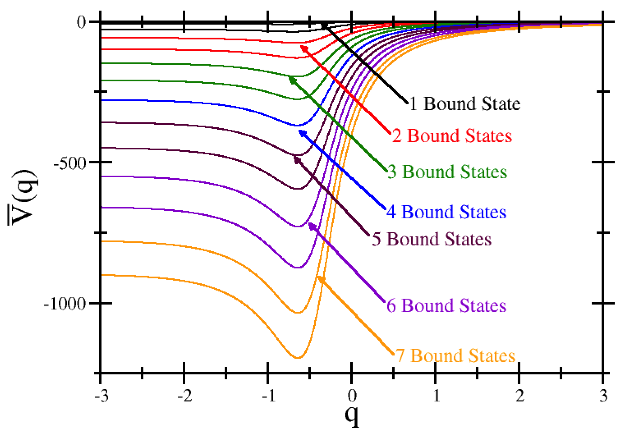
For our numerical examples, we chose cases where the left limit varied, while the right limit was always at 0. To achieve this, we took ${\alpha }_1=1$, ${\alpha }_2=-1$, ${\alpha }_3=1$, $v_1=0$, $v_2=1$, and $v_3+1<-6.85$. This was the case that had at least one bound state. This was because the negative value for $v_3$ requires $\overline{E}<1+v_3$ in order for the far right square root in Equation (140) to be a real number. In this regime, the first term on the right-hand side was small and negative, while the second term was large and positive. The maximal n value we could have if we neglected the small negative terms was then

$$n_{\max }\approx -\frac{{\alpha }_2}{4}\sqrt{\frac{-(1+v_3)}{{\alpha }_1{\alpha }_3}}-\frac{1}{2}=\frac{1}{4}\sqrt{-(1+v_3)}-\frac{1}{2}$$

(142)

for these sets of parameters. One can see we had one bound state for $v_3$ less than about $-5$ (the correct value is $-7.85$), two bound states when $v_3$ was less than about $-37$, three when $v_3$ was less than about $-99$, and so on.

The strategy to compute the results numerically is then straightforward. We set $\zeta$ on a grid. In order to obtain large negative values of q, we needed pick a small step size near $\zeta =0$ because q goes to $-\infty$ only logarithmically in $\zeta$; q and $\zeta$ are related approximately linearly when $\zeta \to \infty$. Then, with this set of $\zeta$ values, we next compute the parametric equations $q\left(\zeta \right)$ from Equation (136) and $V\left(\zeta \right)$ from Equation (133). Then, we plot $V\left(q\right)$ by simply using the corresponding results for q and V. The potentials for these parameters are plotted in Figure 1 (The data for the figure is provided in Supplementary Materials). They all have clear wells where we have bound states. As we decrease $v_3$, the well becomes deeper, which allows for more bound states. The approximate transition points are reported in the caption of Figure 2. The potential becomes more asymmetric as well. As the depth becomes deeper, we anticipate that there would be more bound states, but in all cases, we expect just a finite number of them. As shown in Figure 2, the energy of each bound state decreases approximately linearly with $v_3$. New bound states enter with energies near the left asymptotic limit and then move downward. In addition, the higher-energy bound states have a smaller spacing than the lower-energy ones. This behavior is similar to the behavior seen in the bound states of the Morse potential. We verify the results for the energy eigenstates via an independent “shooting method” code to find the ground states with specific energy eigenvalues. We find that the shooting method (performed on a finite, rather than infinite, domain) produces an energy that agrees to four or more decimal points, confirming all of the numerics.

6. Conclusions

In this work, we describe a different approach to solving the energy eigenvalue problem, which we call single-shot factorization. By introducing an ansatz for the superpotential that is a logarithmic derivative of confluent hypergeometric functions, plus some additional simple functions, we are able to find analytical solutions by inputting an analytically solvable potential and determining the energies and wavefunctions by enforcing appropriate boundary conditions and normalization conditions. The approach can also be used in the converse way by inputting a normalizable eigenfunction and using the factorization to determine the potential. This converse problem is equivalent to Natanzon’s method, but our approach provides a different perspective to this problem, especially with regard to its relationship with supersymmetric quantum mechanics.

In supersymmetric quantum mechanics, or more generally in the conventional factorization method, one forms a factorization chain and a sequence of auxiliary Hamiltonians to solve the problem. In each case, the factorization is performed with a superpotential that is a logarithmic derivative of a ground-state wavefunction, which has no nodes. Instead, in the single-shot factorization approach, there is no factorization chain, no auxiliary Hamiltonians, and each factorization has a superpotential that is singular at the nodes of the wavefunction. This provides another perspective of the energy eigenvalue problem that is different from the Schrödinger equation approach and the conventional factorization method.

In the process of our solution, we found it expedient to require the constraint in Equation (20) to ensure that the potential was independent of the quantization energy. This constraint naturally arose in Natanzon’s work when converting hypergeometric differential equations to the Schrödinger equation. If there happens to be some special form of $M(a,b,\zeta )$ such that $\frac{M(a,b+1,\zeta )}{M(a,b,\zeta )}$ is not dependent on a and b, there might be additional solutions to be uncovered that go beyond what Natanzon discovered. Most likely, any new solution would need to be on a finite and not infinite domain, as it might be easier to enforce the constraint of the potential not depending on the energy for that case.

This work focused exclusively on confluent hypergeometric function representations for the eigenfunctions. It should be possible to extend this work using hypergeometric functions and even Heun functions. Some work in this direction has already been completed from the perspective of supersymmetric quantum mechanics [16]. This indicates that the single-shot factorization method we use here should be able to be extended in these directions. We leave this question for future work.

References

1. Schrödinger, E. Quantisierung als Eigenwertproblem. Ann. Phys. 1926, 384, 361–376. [Google Scholar] [CrossRef]
2. Schrödinger, E. A Method of Determining Quantum-Mechanical Eigenvalues and Eigenfunctions. Proc. R. Irish Acad. A 1940/1941, 46, 9–16. [Google Scholar]
3. Witten, E. Dynamical Breaking of Supersymmetry. Nucl. Phys. B 1981, 188, 513–554. [Google Scholar] [CrossRef]
4. Junker, G. Supersymmetric Methods in Quantum and Statistical Physics; Springer: Berlin/Heidelberg, Germany, 1996. [Google Scholar]
5. Cooper, F.; Khare, A.; Sukhatme, U. Supersymmetry and Quantum Mechanics; World Scientific: Singapore, 2001. [Google Scholar]
6. Lévai, G. A search for shape-invariant solvable potentials. J. Phys. A Math. Gen. 1989, 22, 689–702. [Google Scholar] [CrossRef]
7. Lévai, G. Symmetry in Natanzon-class potentials. Int. J. Theor. Phys. 2015, 54, 2724–2736. [Google Scholar] [CrossRef]
8. Soltész, T.; Pethó, L.F.; Lévai, G. Unified supersymmetric description of shape-invariant potentials within and beyond the Natanzon class. Symmetry 2024, 16, 174. [Google Scholar] [CrossRef]
9. Freericks, J.K.; Mathews, W.N., Jr. Continuum energy eigenstates via the factorization method. Symmetry 2023, 15, 797. [Google Scholar] [CrossRef]
10. Natanzon, G.A. General properties of potentials for which the Schrödinger equation can be solved by means of hypergeometric functions. Theor. Math. Phys. 1979, 38, 146–153. [Google Scholar] [CrossRef]
11. Mathews, W.N., Jr.; Esrick, M.A.; Teoh, Z.Y.; Freericks, J.K. A physicist’s guide to the solution of Kummer’s equation and confluent hypergeometric functions. Condens. Matt. Phys. 2022, 25, 33203. [Google Scholar] [CrossRef]
12. Natanzon, G.A. Study of the one-dimensional Schrödinger equation generated from the hypergeometric equation. Vestn. Leningr. Univ. 1971, 10, 22–28. [Google Scholar]
13. [DLMF] NIST Digital Library of Mathematical Functions. Release 1.1.12. Available online: http://dlmf.nist.gov/ (accessed on 29 December 2023).
14. Dereziński, J.; Wrochna, M. Exactly solvable Schrödinger operators. Ann. Henri Poincare 2011, 12, 397–418. [Google Scholar] [CrossRef]
15. Gradshteyn, I.S.; Ryzhik, I.M. Table of Integrals, Series, and Products, 7th ed.; Academic Press: New York, NY, USA, 2014. [Google Scholar]
16. Ishkhanyan, A.; Krainov, V. Discretization of Natanzon potentials. Eur. Phys. J. Plus. 2016, 131, 342. [Google Scholar] [CrossRef]
Figure 1. Exactly solvable potentials for different  v 3  values ( v 3  became more negative). We plot  v 3 = 10 30 60 100 150 210 280 360 450 550 660 780 , and  900 . The color coding records the number of bound states for each potential well. The well increases in depth, allowing for more bound states. It also becomes more asymmetric.
Symmetry 16 00297 g001
Figure 2. Behavior of the bound state energies as v3 → −∞. One can see that as the potential depth deepens, more bound states are allowed in the system. The newly formed bound states enter at first with the asymptotic value of the left limit, in this case, because it is the lower of the two limits of the potential. The approximate transitions are as follows: two bound states, v3 ≈ −39; three bound states, v3 ≈ −103; four bound states, v3 ≈ −199; five bound states, v3 ≈ −327; six bound states, v3 ≈ −487; and seven bound states, v3 ≈ −679.
Symmetry 16 00297 g002
Disclaimer/Publisher’s Note: The statements, opinions and data contained in all publications are solely those of the individual author(s) and contributor(s) and not of MDPI and/or the editor(s). MDPI and/or the editor(s) disclaim responsibility for any injury to people or property resulting from any ideas, methods, instructions or products referred to in the content.