A Non-Convex Fractional-Order Differential Equation for Medical Image Restoration

Abstract

We propose a new non-convex fractional-order Weber multiplicative denoising variational generalized function, which leads to a new fractional-order differential equation, and prove the existence of a unique solution to this equation. Furthermore, the model is solved using the partial differential equation (PDE) method and the alternating direction multiplier method (ADMM) to verify the theoretical results. The proposed model is tested on some symmetric and asymmetric medical computerized tomography (CT) images, and the experimental results show that the combination of the fractional-order differential equation and the Weber function has better performance in medical image restoration than the traditional model.

1. Introduction

Images are one of the most important ways for human beings to acquire and share information. Nowadays, image processing techniques have been applied to numerous aspects, such as image denoising, image segmentation, and image enhancement. As a matter of fact, the uncertainty of internal and external factors affect the visual quality of the image. Therefore, image denoising is an essential preprocessing step for digital image processing.

Compared to additive noise, multiplicative noise is more destructive and causes more damage to the image, making image recovery more difficult. In recent years, the removal of multiplicative noise has attracted much attention. Multiplicative noise exists in coherent imaging systems, such as laser imaging, ultrasound imaging, and synthetic aperture radar imaging [1,2,3,4,5]. Therefore, the removal of multiplicative noise is of great significance in various image processing methods. The mathematical formulation of such degradation processes can be expressed as follows [6]:

$$f=u\eta$$

(1)

where $f$ is the observed noisy image, $u$ is the noise-free image, and $\eta$ is multiplicative noise. Due to its characteristics, its removal is more difficult and challenging than additive noise. Therefore, multiplicative noise will be investigated in this paper.

At present, researchers have proposed many methods to remove multiplicative noise, such as Lee’s method [7], the scale threshold method [8], and variational methods [1,2]. Among the variational approaches to image reconstruction methods, Rudin, Lions, and Osher [1] first proposed a classical total variation regularization model (RLO) that is effective and simple. However, this method uses total variation (TV) regularization and produces a staircase effect, which can degrade the quality of image restoration. To improve this result, it was proposed in [2] to use higher-order TV (HOTV) as a regular term. It is effective in suppressing the staircase effect when removing noise; however, it can cause blurring of the image edges because it spreads too fast at the edges.

Fractional-order total variation regularization utilizes the properties of fractional-order calculus and takes into account the use of non-local information of the image for reconstruction. Figure 1 shows the amplitude–frequency characteristic curves of each order, from which it can see that the differentiation of each order has a certain enhancing effect on the high-frequency part of the signal, and with increases in order and frequency, the enhancing effect becomes stronger. The differentiation of each order has a certain attenuating effect on the low-frequency part of the signal, and this effect becomes weaker with the decrease in order. The fractional-order TV regularization term is better able to handle the texture details of the image. Therefore, fractional-order TV regularization terms have been considered by many scholars to reduce the step effect. For more details, please refer to [9,10,11,12,13,14,15,16]. In [16], the authors combine a non-convex norm with fractional-order variational to denoise images containing impulse noise, and the model is effective in overcoming the step effect and maintaining neat contours.

All images are eventually perceived by the human visual system. From an imaging perspective, image processing takes visual perception into account, yet most conventional image processing modalities rarely take this into account by weighting background stimuli to influence human perception and response to fluctuations in the intensity of visual signals, which is Weber’s law at work in psychology. Weber’s law was first described by the German physiologist Weber in 1834 [17] and later quantified by the experimental psychologist Fechner, the founder of modern psychophysics. In [18], the authors combined Weber’s law with the classical variational model ROF to propose the Weberized nonlinear TV restoration model, theoretically analyzed it, and experimentally derived that the minimum permissible fluctuation $\delta u$ is larger in the restored image on the region with higher background intensity $u$ and weaker human visual sensitivity. In [19,20], the authors combined Weber with AA [21] and I-div multiplicative denoising models, respectively, and proved experimentally that their proposed model performs well in image denoising. They have shown that for a large range of stimuli $u$, Weber’s law provides a good approximation. Therefore, Weber’s law will be the basis for the development of our model in this paper.

This paper is organized as follows. In Section 2, we review some classic variational models for removing additive noise or multiplicative noise as well as the alternating direction multiplier method (ADMM) algorithm. In Section 3, we propose our new restoration model and prove that the minimum value exists. In Section 4, the ADMM iterative algorithm is introduced for the solution of the proposed model. Some numeric results of the experiments are presented in Section 5, and the paper concludes with Section 6.

2. Model Review and Related Algorithm

In this section, several classical multiplicative denoising models and Weberized total variational restoration models are introduced as well as the alternating direction multiplier method algorithm.

2.1. Multiplicative Denoising Model

2.1.1. The RLO Model

Rudin, Lions, and Osher [1] firstly proposed the denoising model for multiplicative noise (RLO) in 2003, and its basic idea is the same as the ROF model. Both models are used to build a minimization model of energy generalization to remove the noise in the image, and they successfully exploit the intrinsic regularity of the image to reflect the geometrical regularity of the real image from the solution of the model. The RLO model is expressed as follows:

$$\underset{u\in BV\left(\Omega \right)}{min}\left\{E\left(u\right)={\int }_{\Omega }\left|\nabla u\right|dx+{\int }_{\Omega }\left[\lambda \frac{f}{u}+\mu {\left(\frac{f}{u}-1\right)}^2\right]dx\right\}$$

(2)

where $\lambda$ and $\mu$ are the regularization parameters.

The RLO model is a classic variational model for multiplicative Gaussian noise. However, since this model is based on the statistical properties of multiplicative noise, the model is not generalizable to other multiplicative noise.

2.1.2. The AA Model

In 2008, assuming that the noise is a mean gamma noise, Aubert and Aujol [21] derived a data fidelity term based on a maximum a posteriori estimation. Considering gamma noise, a non-convex model, AA model, is proposed:

$$\underset{u\in BV\left(\Omega \right)}{min}\left\{E\left(u\right)={\int }_{\Omega }\left|\nabla u\right|dx+\lambda {\int }_{\Omega }\left(\mathit{log}u+\frac{f}{u}\right)dx\right\}$$

(3)

The only sufficient condition for a minimal solution of this model to exist is $u\in (0, 2f)$.

The AA model can effectively remove gamma multiplicative noise. However, since the AA model’s fidelity term is non-convex, it tends to block the denoising process, resulting in poor denoising.

2.1.3. The SO Model

Shi and Osher [22] proposed a convex variational model using the corresponding relaxation inverse scale space flow as a denoising method by using the data fidelity term of the AA model with ${|log u|}_{BV}$ instead of ${\left|u\right|}_{BV}$ in the regular term part:

$$\underset{w\in BV\left(\Omega \right)}{min}\left\{E\left(w\right)={\int }_{\Omega }\left|\nabla w\right|dx+\lambda {\int }_{\Omega }\left[af{e}^{-w}+\frac{b}{2}{f}^2{e}^{-2w}+\left(a+b\right)w\right]dx\right\}$$

(4)

Here, $w=log u$ and $a, b$ are nonnegative constants.

2.1.4. The I-Divergence Model

Inspired by the AA model, Steidl and Teuber [23] proposed the I-divergence model, also called the generalized Kullback–Leibler divergence (KL divergence) model, in 2010.

I-divergence of $f$ and $u$: $I\left(f,u\right)={\int }_{\Omega }\left(f\mathit{log}\frac{f}{u}-f+u\right)dx$.

Since $f$ is the observed image, ignoring the constant term simplifies the equation to the following: ${\int }_{\Omega }\left(u-flog u\right)$. The model uses general KL divergence, i.e., I-divergence, as the fidelity term, and the total variation as regular term. The mathematical expression is as follows:

$$\underset{u\in BV\left(\Omega \right)}{min}\left\{E\left(u\right)={\int }_{\Omega }\left|\nabla u\right|dx+\lambda {\int }_{\Omega }\left(f\mathit{log}\frac{f}{u}-f+u\right)dx\right\}$$

(5)

The advantage of the Weberized model is that it improves the contrast retained in the image. Now, we introduce several denoising models with the Weberized model.

2.2. The Weberized Denoising Model

2.2.1. The Weberized ROF Denoising Model

In 2003, Jianhong Shen merged Weber’s law with the ROF model proposed by Rudin, Osher, and Fatemi in 1993 and proposed a Weberized classical TV model to remove additive noise [18]:

$$\underset{u\in BV\left(\Omega \right)}{min}\left\{E_w\left[u|f\right]={\int }_{\Omega }{\left|\nabla u\right|}_{w}dx+\frac{\lambda }{2}{\int }_{\Omega }{\left(u-f\right)}^{2}dx\right\}$$

(6)

Here, ${\int }_{\Omega }{\left|\nabla u\right|}_{w}dx={\int }_{\Omega }\frac{|\nabla u|}{u}dx$. The first term is the Weber regularity term. The second term is a non-convex data fidelity term, consistent with the ROF model.

2.2.2. The Weberized AA Denoising Model

Lili Huang, Liang Xiao, and Zhihui Wei [19] proposed an image multiplicative noise removal model based on the combination of Weber’s total variational regularization and the AA model in 2009.

$$\underset{u\in BV\left(\Omega \right)}{min}{E}_w\left[u|f\right]={\int }_{\Omega }{\left|\nabla u\right|}_{w}dx+\lambda {\int }_{\Omega }\left(\frac{f}{u}+\mathit{log}u\right)dx={\int }_{\Omega }\frac{\left|\nabla u\right|}{u}dx+\lambda {\int }_{\Omega }\left(\frac{f}{u}+\mathit{log}u\right)dx$$

(7)

Its corresponding Euler Lagrange equation is expressed as follows:

$$-\frac{1}{u}div\left(\frac{\nabla u}{\left|\nabla u\right|}\right)+\lambda \left(\frac{1}{u}-\frac{f}{u^2}\right)=0$$

(8)

2.2.3. Weberized I-Divergence Denoising Model

In 2023, Xinyao Yu and Donghong Zhao [20] proposed an image multiplicative denoising model combining Weber’s total variation regularization term and the I-div data fidelity term:

$$\underset{u\in BV\left(\Omega \right)}{min}\left\{E\left(u\right)={\int }_{\Omega }\frac{\left|\nabla u\right|}{u}dx+\lambda {\int }_{\Omega }\left(u-f\mathit{log}u\right)dx\right\}$$

(9)

Its corresponding Euler Lagrange equation is expressed as follows:

$$-\frac{1}{u}div\left(\frac{\nabla u}{\left|\nabla u\right|}\right)+\lambda \left(1-\frac{f}{u}\right)=0$$

(10)

2.3. ADMM Introduction

The alternating direction multiplier method(ADMM) [24,25] combines the decomposability of the pairwise ascent method with the superior convergence of the multiplier method. A recent study [26] revealed that the ADMM algorithm is also closely related to the Douglas–Rachford splitting method, Spingain’s partial inverse method, Dykstra’s alternating projection, and the splitting Bregman iterative algorithm. Given a constrained optimization problem, the equation is denoted as follows:

$$\underset{x,z}{min} \left\{f\left(x\right)+g\left(z\right)\right\} s.t. Ax+Bz=C$$

where $x\in R^n, z\in R^n, A\in R^{m\times n}, B\in R^{m\times n}, \mathrm{a}\mathrm{n}\mathrm{d} C\in R^m$. Assume also that $f\left(·\right), g(·)$ are convex. The above constrained optimization problem can be written as:

• the objective function: $f\left(x\right)+g\left(z\right)$ $x\in R^n,z\in R^n$.
• the restrictive condition: $Ax+Bz=C$.

Its augmented Lagrangian function is expressed as follows: $L\left(x,z;\tau \right)=f\left(x\right)+g\left(z\right)+{\tau }^T\left(Ax+Bz-C\right)+\frac{\rho }{2}{‖Ax+Bz-C‖}_2^2$, where $\frac{\rho }{2}{\left|\right|Ax+Bz-C\left|\right|}_2^2$ is the penalty, $\tau$ is the augmented Lagrange multiplier, and $\rho$ is an augmentation penalty parameter.

Using the alternating iteration method to find the minima for the augmented and generalized Lagrange equations, the following ADMM iteration is obtained:

$$\left\{\begin{array}{c}{x}^{k+1}=\mathrm{a}\mathrm{r}\mathrm{g}min L\left(x,z^k,{\tau }^k\right)\\ z^{k+1}=\mathrm{a}\mathrm{r}\mathrm{g}min L\left(x^{k+1},z,{\tau }^k\right)\\ {\tau }^{k+1}={\tau }^k+\rho \left(A{x}^{k+1}+B{z}^{k+1}-C\right)\end{array}\right.$$

(11)

The ADMM method can transform the complex multi-optimization variable problem into a simple single optimization variable subproblem, so that different solutions can be adopted for different subproblems. Moreover, the experimental results of ADMM method for the quadratic penalty term are generally convergent [25,27]. Therefore, this paper uses ADMM method to solve the proposed model.

3. Modeling and Analysis

In this section, we use the Grünwald-Letnikov(G-L) fractional-order derivatives, combine Weber’s law with the I-div model to construct a multiplicative denoising model of fractional order, and provide a proof of the existence of uniqueness of the model in this paper.

3.1. The Proposed Model

Combining Weberized I-divergence denoising model [20] and the fractional-order variational model, we propose the model of this paper:

$$\underset{u\in S\left(\Omega \right)}{min}E\left(u\right)={\int }_{\Omega }\frac{\left|{\nabla }^{\alpha }u\right|}{u}dx+\lambda {\int }_{\Omega }\left(u-f\mathit{log}u\right)dx$$

(12)

where $\alpha$ is a fractional order and $\lambda$ is the regularization parameter.

The first term is the regularity term, which is a fractional-order Weber variation term. The second term is the data fidelity term, which is derived from the constraints, and ensures that the denoised image and the observed image are still as consistent as possible in terms of information other than noise. The two terms are minimized in terms of the difference between the noise signal interference, i.e., it is hoped that the loss of information will be minimized. Here, $\lambda$ is the regularization parameter that is used to balance the regularity term and the data fidelity term.

The space of solutions is noted as follows: $S\left(\Omega \right)=\left\{u>0|u\in L^1\left(\Omega \right),{TV}^{\alpha }\left(\mathit{log}u\right)<\mathrm{\infty }\right\}$.

3.2. Theoretical Analyses

3.2.1. Existence

Proof of boundedness of a solution is provided before proving the existence of a solution to the model.

Lemma 1 (Boundness).

Let $f\in L^{\infty }\left(\Omega \right)$ and $\underset{\Omega }{inf} f>0$. If the model has a solution $v$, then $\underset{\Omega }{inf} f<v<\underset{\Omega }{sup} f$.

Proof of Lemma 1.

Note $\alpha =\underset{\Omega }{inf}f$, $\beta =\underset{\Omega }{sup}f$. When $u>f$, function $u-f\mathit{log}u$ increases monotonically, so there is ${\int }_{\Omega }\left(\mathit{inf}\left(u,\beta \right)-f\mathit{log}\mathit{inf}\left(u,\beta \right)\right)dx\le {\int }_{\Omega }\left(u-f\mathit{log}u\right)dx$.

Moreover, based on Lemma 1 in the literature [28], ${TV}^{\alpha }\left(\mathit{log}\mathit{inf}\left(u,\beta \right)\right)\le {TV}^{\alpha }\left(\mathit{log}u\right)$ exists.

Thus, there is $E\left(\mathit{inf}\left(u,\beta \right)\right)\le E\left(u\right)$, and the equation holds if and only if $u\le \beta$.

Since $v$ is the minimum solution of this model, the equation holds when $u=v$ and hence $v\le \beta$.

Similarly, if $E\left(u\right)\le E\left(sup\right(u,\alpha \left)\right)$, then $v\ge \alpha$ can be obtained.

In summary, $\underset{\Omega }{inf}f<v<\underset{\Omega }{sup}f$. □

In the following, we will give an existence proof for the solution of the model.

Lemma 2 (Existence).

Let $f\in L^{\infty }\left(\Omega \right)$ and $\underset{\Omega }{inf} f>0$, then the optimization problem has at least one solution in its solution space $S\left(\Omega \right)$.

Proof of Lemma 2.

Define $\alpha =\underset{\Omega }{inf} f, \beta =\underset{\Omega }{sup} f$. Since there is $u\equiv \beta \in S\left(\Omega \right)$, the solution space $S\left(\Omega \right)$ is nonempty [18].

Set $\left\{u_n\right\}\in S\left(\Omega \right)$ as the minimizing sequence of this optimization problem. Based on the boundedness, there is $\alpha \le u_n\le \beta$; thus, ${\int }_{\Omega }\frac{\left|{\nabla }^{\alpha }u\right|}{\beta }dx\le {\int }_{\Omega }\frac{\left|{\nabla }^{\alpha }{u}_n\right|}{u_n}dx\le {\int }_{\Omega }\frac{\left|{\nabla }^{\alpha }u\right|}{\alpha }dx$.

Since $\left\{u_n\right\}$ is a bounded sequence in Banach space ${BV}^{\alpha }\left(\Omega \right)$, the space of bounded variational functions ${BV}^{\alpha }\left(\Omega \right)$ be defined as ${BV}^{\alpha }\left(\Omega \right)=\{f:f\in L^1(\Omega ),{TV}^{\alpha }(f)<\infty \}$, forming Banach spaces under the BV norm ${‖f‖}_{BV}={‖f‖}_{L^1}+{TV}^{\alpha }\left(f\right)$. Because $\Omega$ is bounded, ${‖u_n‖}_{L^1}<\infty$.

Furthermore, based on the definition of the minimization sequence of $\left\{u_n\right\}$, a constant $C>0$ exists, so $E\left(u_n\right)\le C$. According to ${TV}^{\alpha }(log u_n)<\infty$, and when $u_n=f$, ${\int }_{\Omega }\left(u_n-f log u_n\right)dx$ can hit the minimum ${\int }_{\Omega }\left(f-f\mathit{log}f\right)dx$. Thus, ${TV}^{\alpha }\left(u_n\right)<C$.

Consequently, $\left\{u_n\right\}$ is uniformly bounded in space ${BV}^{\alpha }\left(\Omega \right)$ with respect to $n$. Based on the tightness of ${BV}^{\alpha }\left(\Omega \right)$ space, there exist subcolumns of $\left\{u_n\right\}$ (still $\left\{u_n\right\}$ is denoted for convenience) and a function $u$ in the space ${BV}^{\alpha }\left(\Omega \right)$ that $\left\{u_n\right\}$ converges strongly to $u$ in $L^1\left(\Omega \right)$-space, i.e., $u_n\left(x\right)\stackrel{n\to \infty }{\to }u\left(x\right)$, a.e. $x\in \Omega$.

Using the Lebesgue control convergence theorem, there is $\underset{n\to \mathrm{\infty }}{lim}{\int }_{\Omega }\left(u_n-flog{u}_n\right)dx={\int }_{\Omega }\left(u-f\mathit{log}u\right)dx$.

Let $w_n=log{u}_n$, $w=logu$, then $w_n\stackrel{n\to \mathrm{\infty }}{\to }w$, a.e. $x\in \Omega$.

Set $\overrightarrow{p}=(p_1,p_2)\in C_0^{\alpha }(\Omega ,R^2)$ is a vector-valued function, and $‖\overrightarrow{p}‖=\sqrt{{p_1}^2+{p_2}^2}\le 1$. Then, $w_n{\nabla }^{\alpha }·\overrightarrow{p}\stackrel{n\to \mathrm{\infty }}{\to }w{\nabla }^{\alpha }·\overrightarrow{p}$, $\left|w_n{\nabla }^{\alpha }·\overrightarrow{p}\right|\le \left|w_n\right|·\left|{\nabla }^{\alpha }·\overrightarrow{p}\right|\le \mathit{log}\beta ·\left|{\nabla }^{\alpha }·\overrightarrow{p}\right|$ a.e. $x\in \Omega$.

Since $\overrightarrow{p}$ is tightly supported, therefore, function $w_n{\nabla }^{\alpha }·\overrightarrow{p}$ belongs to space $L^1\left(\Omega \right)$.

Using the Lebesgue control convergence theorem again, the following equations are obtained:

$$\underset{n\to \infty }{lim}{\int }_{\Omega }{w}_n{\nabla }^{\alpha }·\overrightarrow{p}dx={\int }_{\Omega }w{\nabla }^{\alpha }·\overrightarrow{p}dx$$

(13)

$$\underset{n\to \infty }{lim}{\int }_{\Omega }{\nabla }^{\alpha }{w}_n·\overrightarrow{p}dx={\int }_{\Omega }{\nabla }^{\alpha }w·\overrightarrow{p}dx$$

(14)

According to the lower semicontinuity of the function [29], the following equations are obtained:

$${\int }_{\Omega }{\nabla }^{\alpha }w·\overrightarrow{p}dx\le \underset{n\to \infty }{lim}\mathit{inf}{\int }_{\Omega }{\nabla }^{\alpha }{w}_n·\overrightarrow{p}dx$$

(15)

$${\int }_{\Omega }\left|{\nabla }^{\alpha }w·\overrightarrow{p}\right|dx\le \underset{n\to \infty }{lim}\mathit{inf}{\int }_{\Omega }\left|{\nabla }^{\alpha }{w}_n·\overrightarrow{p}\right|dx$$

(16)

According to $‖\overrightarrow{p}‖=\sqrt{{p_1}^2+{p_2}^2}\le 1$, it is known that

$${\int }_{\Omega }\left|{\nabla }^{\alpha }w\right|dx\le \underset{n\to \infty }{lim}\mathit{inf}{\int }_{\Omega }\left|{\nabla }^{\alpha }{w}_n\right|dx$$

(17)

Because ${\int }_{\Omega }\frac{\left|{\nabla }^{\alpha }u\right|}{u}dx={TV}^{\alpha }\left(\mathit{log}u\right)={\int }_{\Omega }\left|{\nabla }^{\alpha }w\right|dx$, the above equations can be combined to yield $E\left(u\right)\le \underset{n\to \mathrm{\infty }}{lim}infE\left(u_n\right)$.

Since $\left\{u_n\right\}$ is a minimization sequence, $u$ is the minimum solution to the optimization problem. Thus, there is $u\in S\left(\Omega \right)$. □

The model is non-convex, so it is not straightforward to understand that the minimum solution is unique [30]. The uniqueness of the minimum solution of its model will be proven below.

To prove uniqueness, there is the following lemma.

Lemma 3.

There exists a function $\phi \left(u\right):(0,\infty )\to (0,\infty )$ of $C^1$, $J\left[u\right]={\int }_{\Omega }\phi \left(u\right)\left|{\nabla }^{\alpha }u\right|dx$. Then, there is an Euler-Lagrange difference of $J\left[u\right]$: $\frac{\partial J}{\partial u}=\overline{{(-1)}^{\alpha }}\phi \left(u\right){div}^{\alpha }\left(\frac{{\nabla }^{\alpha }u}{\left|{\nabla }^{\alpha }u\right|}\right)+\frac{\phi \left(u\right)}{\left|{\nabla }^{\alpha }u\right|}·\frac{\partial u}{\partial \overrightarrow{n}}{|}_{\partial \Omega }$.

Proof of Lemma 3.

According to the definition of difference, one can obtain the following:

$$\begin{array}{}\delta J={\int }_{\Omega }\left({\phi }^{\prime }\left(u\right)\left|{\nabla }^{\alpha }u\right|·\delta u+\phi \left(u\right)·\frac{{\nabla }^{\alpha }u}{\left|{\nabla }^{\alpha }u\right|}·\delta \left({\nabla }^{\alpha }u\right)\right)dx\\ ={\int }_{\Omega }{\phi }^{\prime }\left(u\right)\left|{\nabla }^{\alpha }u\right|·\delta udx+{\int }_{\partial \Omega }\delta u·\frac{\phi \left(u\right)}{\left|{\nabla }^{\alpha }u\right|}·\frac{\partial u}{\partial \overrightarrow{n}}ds\\ -{\int }_{\Omega }\delta u·\nabla ·\left(\phi \left(u\right)\frac{{\nabla }^{\alpha }u}{\left|{\nabla }^{\alpha }u\right|}\right)dx\\ ={\int }_{\Omega }\left[{\phi }^{\prime }\left(u\right)\left|{\nabla }^{\alpha }u\right|-\nabla ·\left(\phi \left(u\right)\frac{{\nabla }^{\alpha }u}{\left|{\nabla }^{\alpha }u\right|}\right)\right]·\delta udx\\ +{\int }_{\partial \Omega }\delta u·\frac{\phi \left(u\right)}{\left|{\nabla }^{\alpha }u\right|}·\frac{\partial u}{\partial \overrightarrow{n}}ds\\ ={\int }_{\Omega }-\phi \left(u\right)\nabla ·\left(\frac{{\nabla }^{\alpha }u}{\left|{\nabla }^{\alpha }u\right|}\right)·\delta udx+{\int }_{\partial \Omega }\frac{\phi \left(u\right)}{\left|{\nabla }^{\alpha }u\right|}·\frac{\partial u}{\partial \overrightarrow{n}}·\delta uds\\ ={\int }_{\Omega }\overline{{(-1)}^{\alpha }}\phi \left(u\right){div}^{\alpha }\left(\frac{{\nabla }^{\alpha }u}{\left|{\nabla }^{\alpha }u\right|}\right)·\delta udx+{\int }_{\partial \Omega }\frac{\phi \left(u\right)}{\left|{\nabla }^{\alpha }u\right|}·\frac{\partial u}{\partial \overrightarrow{n}}·\delta uds\end{array}$$

where $ds$ is the arc length element of the boundary and $\overrightarrow{n}$ is the outer normal of the boundary $\partial \Omega$.

Thus, $\frac{\partial J}{\partial u}=\overline{{(-1)}^{\alpha }}\phi \left(u\right){div}^{\alpha }\left(\frac{{\nabla }^{\alpha }u}{\left|{\nabla }^{\alpha }u\right|}\right)+\frac{\phi \left(u\right)}{\left|{\nabla }^{\alpha }u\right|}·\frac{\partial u}{\partial \overrightarrow{n}}{|}_{\partial \Omega }$. □

3.2.2. Uniqueness

Theorem 1 (Uniqueness).

Let $f\in L^{\infty }\left(\Omega \right)$ and $\underset{\Omega }{inf} f>0$, then the solution of this optimization problem in its solution space $S\left(\Omega \right)$ is unique.

Proof of Theorem 1.

According to Lemma 3, it follows that the Euler–Lagrange equation for this model is expressed as noted below:

$$\overline{{(-1)}^{\alpha }}\frac{1}{u}{div}^{\alpha }\left(\frac{{\nabla }^{\alpha }u}{\left|{\nabla }^{\alpha }u\right|}\right)+\lambda \left(1-\frac{f}{u}\right)=0, \frac{\partial u}{\partial \overrightarrow{n}}=0 x\in \partial \Omega$$

(18)

Because $u>0$, the above equation can be transformed into the following:

$$\overline{{(-1)}^{\alpha }}{div}^{\alpha }\left(\frac{{\nabla }^{\alpha }u}{\left|{\nabla }^{\alpha }u\right|}\right)+\lambda \left(u-f\right)=0, \frac{\partial u}{\partial \overrightarrow{n}}=0 x\in \partial \Omega$$

(19)

Set $F^{\prime }\left(u\right)=\lambda \left(u-f\right)$, then $F^{″}\left(u\right)=\lambda$, $F\left(u\right)=\lambda \left(\frac{u^2}{2}-fu\right)$.

Let $E_w\left(u\right)={TV}^{\alpha }\left(u\right)+F\left(u\right)$, then the Euler–Lagrange equations for $E_w\left(u\right)$ and $E\left(u\right)$ are the same. Hence, the uniqueness for the minimum solution is the same.

Since $F^{″}\left(u\right)=\lambda$ and $\lambda >0$, then $F\left(u\right)$ is a strictly convex function. Because ${TV}^{\alpha }\left(u\right)$ is convex (but not strictly convex), $E_w\left(u\right)$ is convex. Based on the existence of a minimal solution, it is thus obtained that the minimal solution of $E_w\left(u\right)$ is unique; therefore, the minimal solution of $E\left(u\right)$ is also unique. □

4. Numerical Methods

4.1. The Gradient Descent Method

In this section, we solve the model of this paper using partial differential equations, which is a classical method for image denoising.

According to Lemma 3 and the uniqueness proof, the corresponding Euler–Lagrange Equation (18) for this model is equivalent to Equation (19). The corresponding diffusion equations are expressed as follows:

$$\frac{\partial \mathrm{u}}{\partial \mathrm{t}}=-\overline{{(-1)}^{\alpha }}\frac{1}{u}{div}^{\alpha }\left(\frac{{\nabla }^{\alpha }u}{\left|{\nabla }^{\alpha }u\right|}\right)-\lambda \left(1-\frac{f}{u}\right)$$

(20)

$$\frac{\partial \mathrm{u}}{\partial \mathrm{t}}=-\overline{{(-1)}^{\alpha }}{div}^{\alpha }\left(\frac{{\nabla }^{\alpha }u}{\left|{\nabla }^{\alpha }u\right|}\right)-\lambda \left(u-f\right)$$

(21)

We propose a new energy functional:

$$E_w\left(u\right)={TV}^{\alpha }\left(u\right)+F\left(u\right)={\int }_{\Omega }\left|{\nabla }^{\alpha }u\right|dx+\lambda {\int }_{\Omega }(\frac{u^2}{2}-fu)dx$$

(22)

One can derive Equation (19) as the Euler–Lagrange equation for (22), so the optimization model (22) has a solution satisfying Equation (19).

Equations (18) and (19) are equivalent; thus, it can be concluded that the optimization problems (12) and (22) have the same Euler–Lagrange equations. The solution of model (12) is also the solution of optimization problem (22); therefore, (12) and (21) are equivalent.

Equation (22) can be viewed as an alternative function to Equation (12) of Weber’s variational minimization problem. Equation (22) is strictly convex and therefore has a unique minimal value. The problem of finding the minima of Equation (12) can be converted into finding the minima of Equation (22).

The iterative format for the solution of the Euler–Lagrange equation is given in the following.

Let $h$ denote the step size of the grid, and generally let $h$ be $1$ in the iteration; denote the time step of the iteration by $∆t$. The differential form of the derivative of the pixel point at $\left(i,j\right)$ with respect to the auxiliary variable time $t$ can be obtained:

$$\frac{\partial u}{\partial t}=\frac{u^{n+1}(i,j)-u^n(i,j)}{∆t}$$

(23)

where $u^n(i,j)$ is the gray value of the pixel point at $\left(i,j\right)$ in the $n$th iteration.

Combining Equation (20) with Equation (23), the iterative form of Equation (12) under the partial differential equation method can be obtained:

$$u^{n+1}(i,j)=u^n(i,j)+∆t\left[-\overline{{(-1)}^{\alpha }}\frac{1}{u^n}{div}^{\alpha }\left(\frac{{\nabla }^{\alpha }{u}^n}{\left|{\nabla }^{\alpha }{u}^n\right|}\right)-\lambda \left(1-\frac{f}{u^n}\right)\right]$$

(24)

During the experiments, it was found that the gradient modes of the images would appear to have very small values, which were directly processed by the computer as $0$ with errors. Therefore, the model was improved using “arithmetic underflow” technique, i.e., adding zero point zero one to the denominator avoids the above problem during the iteration process. This modification proved to be effective and reasonable in the experiments.

In this paper, we choose different values of parameter $\lambda$ and carry out numerous experiments to determine the best value of $0.05$.

The steps of solving the model with PDE are shown in Algorithm 1.

Algorithm 1: Partial Differential Equation Methods (PDE)

Initialization: $u^0=f$. Parameters: $\lambda =0.05$, stopping condition Maximum number of iteration: $\mathrm{I}\mathrm{t}\mathrm{e}\mathrm{r}\mathrm{M}\mathrm{a}\mathrm{x}$. Iteration: For each $n=0,1,2,3,\dots$, compute $u^{n+1}(i,j)=u^n(i,j)+∆t\left[-\overline{{(-1)}^{\alpha }}\frac{1}{u^n}{div}^{\alpha }\left(\frac{{\nabla }^{\alpha }{u}^n}{\left|{\nabla }^{\alpha }{u}^n\right|}\right)-\lambda \left(1-\frac{f}{u^n}\right)\right]$ Let $n=n+1$, go to step 3; If $n=IterMax$ is satisfied, output the recovered image $u$.

4.2. The ADMM Algorithm

Based on the format of the optimization problem equation solved using the ADMM method, the total variational image recovery regularization model can be equivalently rewritten by introducing the auxiliary variable $d$ as follows:

$$\underset{u,d}{min}{\int }_{\Omega }ddx+\lambda {\int }_{\Omega }\left(u-flogu\right)dx$$

$$\mathrm{s}.\mathrm{t}.\frac{\left|{\nabla }^{\alpha }u\right|}{u}=d$$

Its corresponding augmented Lagrangian equation is expressed as follows:

$$L\left(u,d;b\right)={\int }_{\Omega }ddx+\lambda {\int }_{\Omega }\left(u-flogu\right)dx+\frac{\mu }{2}{‖\frac{\left|{\nabla }^{\alpha }u\right|}{u}-d+b‖}_2^2-\frac{\mu }{2}{\left|\left|b\right|\right|}_2^2$$

(25)

where $b=\left(b_x,b_y\right)\in X\times X$ is Lagrange multiplier. Here, $\mu >0$ provides sufficiently large penalty parameters.

The ADMM uses an alternating iterative updating method, which can be obtained by decomposing the generalized Lagrangian equation into the following three subproblems:

$$u-\mathrm{s}\mathrm{u}\mathrm{b}\mathrm{p}\mathrm{r}\mathrm{o}\mathrm{b}\mathrm{l}\mathrm{e}\mathrm{m}:u^{k+1}=\mathrm{a}\mathrm{r}\mathrm{g}\underset{u}{min} \lambda {\int }_{\Omega }\left(u-flogu\right)dx+\frac{\mu }{2}{‖\frac{\left|{\nabla }^{\alpha }u\right|}{u}-d^k+b^k‖}_2^2$$

$$d-\mathrm{s}\mathrm{u}\mathrm{b}\mathrm{p}\mathrm{r}\mathrm{o}\mathrm{b}\mathrm{l}\mathrm{e}\mathrm{m}:d^{k+1}=\mathrm{a}\mathrm{r}\mathrm{g}\underset{d}{min} {\int }_{\Omega }ddx+\frac{\mu }{2}{‖\frac{\left|{\nabla }^{\alpha }{u}^{k+1}\right|}{u^{k+1}}-d+b^k‖}_2^2$$

$$b-\mathrm{s}\mathrm{u}\mathrm{b}\mathrm{p}\mathrm{r}\mathrm{o}\mathrm{b}\mathrm{l}\mathrm{e}\mathrm{m}:b^{k+1}=b^k+\left(\frac{\left|{\nabla }^{\alpha }{u}^{k+1}\right|}{u^{k+1}}-d^{k+1}\right)$$

The above subproblem is solved below:

• Solve $u-\mathrm{s}\mathrm{u}\mathrm{b}\mathrm{p}\mathrm{r}\mathrm{o}\mathrm{b}\mathrm{l}\mathrm{e}\mathrm{m}$

The $u-\mathrm{s}\mathrm{u}\mathrm{b}\mathrm{p}\mathrm{r}\mathrm{o}\mathrm{b}\mathrm{l}\mathrm{e}\mathrm{m}$ can be solved using Fourier transformation and Fourier inverse transformation; the discrete case yields the following equation:

$$\left[\lambda I+\mu {\left({\nabla }^{\alpha }\right)}^{*}\left({\nabla }^{\alpha }\right)\right]u^{k+1}=\lambda f+\mu {\left({\nabla }_x^{\alpha }\right)}^{*}\left(d_x^k-b_x^k\right)+\mu {\left({\nabla }_y^{\alpha }\right)}^{*}\left(d_y^k-b_y^k\right)$$

(26)

Fourier transformation of both sides of the equation at the same time yields the following:

$$\left(\lambda F\right(I)+\mu (F{\left({\nabla }_x^{\alpha }\right)}^{*}·F\left({\nabla }_x^{\alpha }\right)+F{\left({\nabla }_y^{\alpha }\right)}^{*}·F\left({\nabla }_y^{\alpha }\right)\left)\right)·F\left(u^{k+1}\right)=\lambda F\left(f\right)+\mu (F{\left({\nabla }_x^{\alpha }\right)}^{*}·F(d_x^k-b_x^k)+F{\left({\nabla }_y^{\alpha }\right)}^{*}·F(d_y^k-b_y^k\left)\right)$$

(27)

where $F$—2D Fourier transform; $·$—Dotwise multiplication between matrices; and $I$—all 1 Matrix.

This is then solved for using Fourier inverse transformation, which yields the following:

$$u^{k+1}=F^{-1}\left(\frac{\lambda F\left(f\right)+\mu (F{\left({\nabla }_x^{\alpha }\right)}^{*}·F(d_x^k-b_x^k)+F{\left({\nabla }_y^{\alpha }\right)}^{*}·F(d_y^k-b_y^k\left)\right)}{\lambda F\left(I\right)+\mu \left(F{\left({\nabla }_x^{\alpha }\right)}^{*}·F\left({\nabla }_x^{\alpha }\right)+F{\left({\nabla }_y^{\alpha }\right)}^{*}·F\left({\nabla }_y^{\alpha }\right)\right)}\right)$$

(28)

• Solve $d-\mathrm{s}\mathrm{u}\mathrm{b}\mathrm{p}\mathrm{r}\mathrm{o}\mathrm{b}\mathrm{l}\mathrm{e}\mathrm{m}$

The solution of $d-\mathrm{s}\mathrm{u}\mathrm{b}\mathrm{p}\mathrm{r}\mathrm{o}\mathrm{b}\mathrm{l}\mathrm{e}\mathrm{m}$ can be obtained using the soft threshold operator.

$$d^{k+1}=S_{\frac{1}{\mu }}\left(\frac{\left|{\nabla }^{\alpha }{u}^{k+1}\right|}{u^{k+1}}+b^k\right)$$

(29)

Here, $S_{\tau }\left(x\right)=\max \left(\left|x\right|-\tau ,0\right)·\frac{x}{\left|x\right|}$, when $\left|x\right|=0$, there is $\frac{x}{\left|x\right|}=0$.

Let $\tau =\frac{1}{\mu }$, $x=\frac{\left|{\nabla }^{\alpha }{u}^{k+1}\right|}{u^{k+1}}+b^k$, then

$$d^{k+1}=S_{\frac{1}{\mu }}\left(\frac{\left|{\nabla }^{\alpha }{u}^{k+1}\right|}{u^{k+1}}+b^k\right)=\max \left(\left|\frac{\left|{\nabla }^{\alpha }{u}^{k+1}\right|}{u^{k+1}}+b^k\right|-\frac{1}{\mu },0\right)·\frac{\frac{\left|{\nabla }^{\alpha }{u}^{k+1}\right|}{u^{k+1}}+b^k}{\left|\frac{\left|{\nabla }^{\alpha }{u}^{k+1}\right|}{u^{k+1}}+b^k\right|}$$

(30)

The steps of solving the model with ADMM are shown in Algorithm 2.

Algorithm 2: FWADMM (Fractional-order Weber I-div model)

$\mathrm{Initialization}: u^0=f$$, d^0=(d_x^0,d_y^0)=\left(\mathrm{0,0}\right)$$, b^0=(b_x^0,b_y^0)=\left(\mathrm{0,0}\right)$ $\mathrm{Parameters}: \mathsf{\lambda }$$, \mu$, stopping condition $tol$ or Maximum number of iterations: $IterMax$. Iteration: For each $k=0, 1, 2, 3, \dots$, compute $u^{k+1}=F^{-1}\left(\frac{\lambda F\left(f\right)+\mu (F{\left({\nabla }_x^{\alpha }\right)}^{*}·F(d_x^k-b_x^k)+F{\left({\nabla }_y^{\alpha }\right)}^{*}·F(d_y^k-b_y^k)}{\lambda I+\mu \left(F{\left({\nabla }_x^{\alpha }\right)}^{*}·F\left({\nabla }_x^{\alpha }\right)+F{\left({\nabla }_y^{\alpha }\right)}^{*}·F\left({\nabla }_y^{\alpha }\right)\right)}\right)$ $d^{k+1}=S_{\frac{1}{\mu }}\left(\frac{\left|{\nabla }^{\alpha }{u}^{k+1}\right|}{u^{k+1}}+b^k\right)=\max \left(\left|\frac{\left|{\nabla }^{\alpha }{u}^{k+1}\right|}{u^{k+1}}+b^k\right|-\frac{1}{\mu },0\right)·\frac{\frac{\left|{\nabla }^{\alpha }{u}^{k+1}\right|}{u^{k+1}}+b^k}{\left|\frac{\left|{\nabla }^{\alpha }{u}^{k+1}\right|}{u^{k+1}}+b^k\right|}$ $b^{k+1}=b^k+\left(\frac{\left|{\nabla }^{\alpha }{u}^{k+1}\right|}{u^{k+1}}-d^{k+1}\right)$ Let $k=k+1$ go to step 3. If $\frac{{‖u^{k+1}-u^k‖}_2}{{‖u^k‖}_2}\le tol$ or $k=IterMax$ is satisfied, output the recovered image $u$.

5. Numerical Results

In this section, some numerical experiments on medical images and natural images show the performance of our proposed model, expanding the application field of the model. In the following section, we will present several objective evaluation criteria for testing the effect of restoring an image.

5.1. Model Evaluation Metrics

Suppose the image size is $M\times N$, the gray value before denoising is $f$, and the gray value after denoising is $\widehat{u}$. There are the following common metrics:

1.

Mean-Square Error (MSE)

$$MSE=\frac{1}{M\times N}\sum _{m=1}^M\sum _{n=1}^N{\left(f-\widehat{u}\right)}^2$$

(31)

2.

Signal-to-Noise Ratio (SNR)

$$SNR=10·{log}_{10}\frac{\sum _{m=1}^M\sum _{n=1}^N{f}^2}{\sum _{m=1}^M\sum _{n=1}^N{\left(f-\widehat{u}\right)}^2}$$

(32)

3.

Structural Similarity (SSIM)

$$SSIM=\frac{\left(2{\mu }_f{\mu }_{\widehat{u}}+c_1\right)(2{\sigma }_{f\widehat{u}}+c_2)}{({\mu }_f^2+{\mu }_{\widehat{u}}^2+c_1)({\sigma }_f^2+{\sigma }_{\widehat{u}}^2+c_2)}$$

(33)

where ${\mu }_f$ and ${\mu }_{\widehat{u}}$ are the means of $f$ and $\widehat{u}$, respectively; ${\sigma }_f^2$ and ${\sigma }_{\widehat{u}}^2$ are the variances of $f$ and $\widehat{u}$, respectively; ${\sigma }_{f\widehat{u}}$ is the covariance of $f$ and $\widehat{u}$; and $c_1$ and $c_2$ are constants used to maintain stability.

4.

Peak Signal-to-Noise Ratio (PSNR)

$$PSNR=10·{log}_{10}\frac{{255}^2}{\frac{1}{M\times N}\sum _{m=1}^M\sum _{n=1}^N{\left(f-\widehat{u}\right)}^2}$$

(34)

There are many more such quantitative indicators. It can be seen that PSNR is calculated from MSE, which tends to differ from human subjective feeling and has low relevance. PSNR is both simple and intuitive and matches human subjective feeling. Currently, the Peak Signal-to-Noise Ratio (PSNR) and structural similarity (SSIM) are the most commonly used objective standards for measuring image quality, and the higher the values, the better the image denoising effect. In this paper, we mainly use the PSNR and SSIM to evaluate the image denoising.

All the tests are performed under Windows 10 and MATLAB R2017b running on a PC with an Intel(R) Core(TM) i5-8250U CPU at 1.60 GHz with 4.0 GB of RAM.

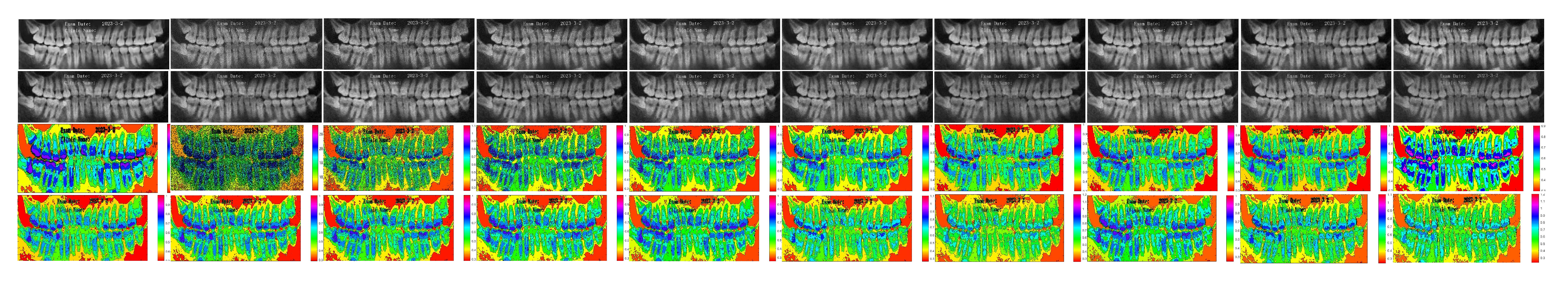
5.2. Numerical Simulations on Medical Images

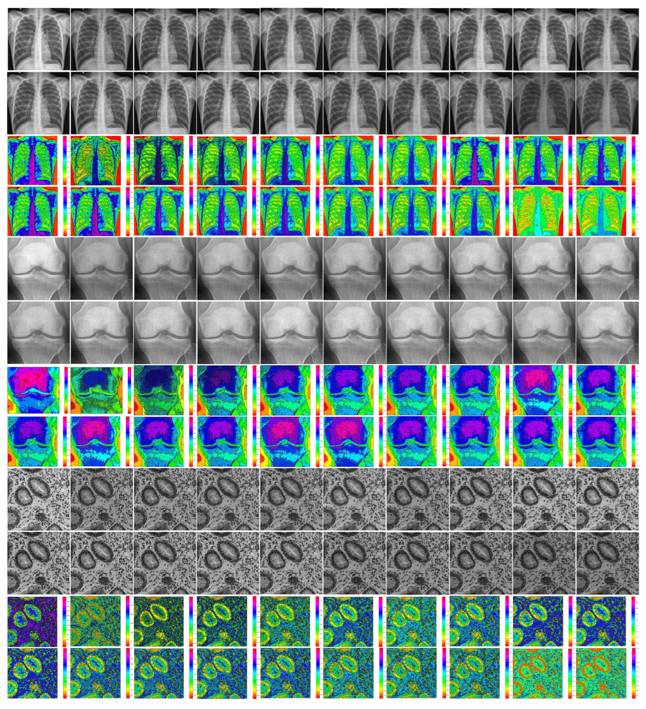
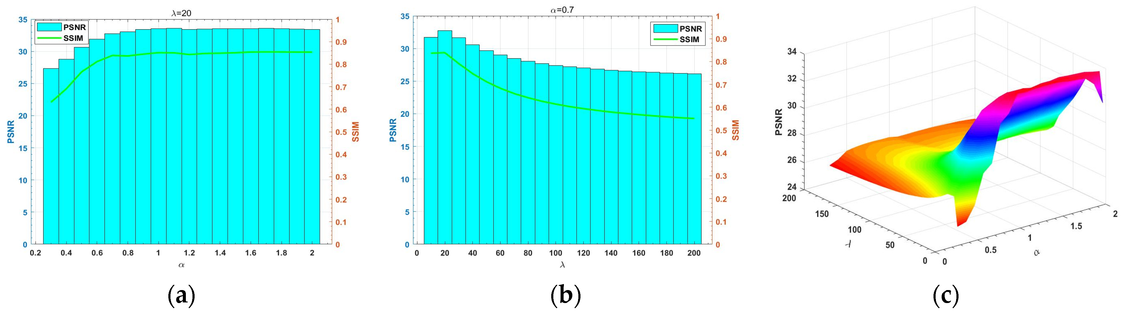
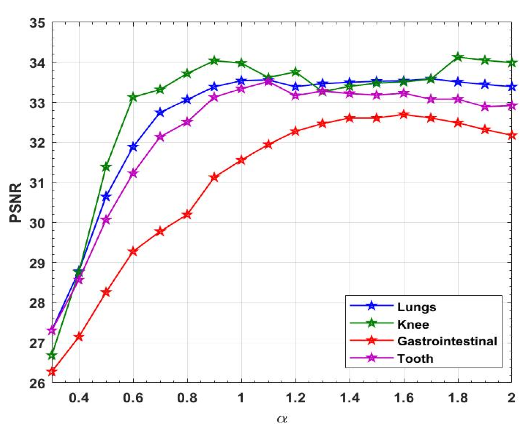
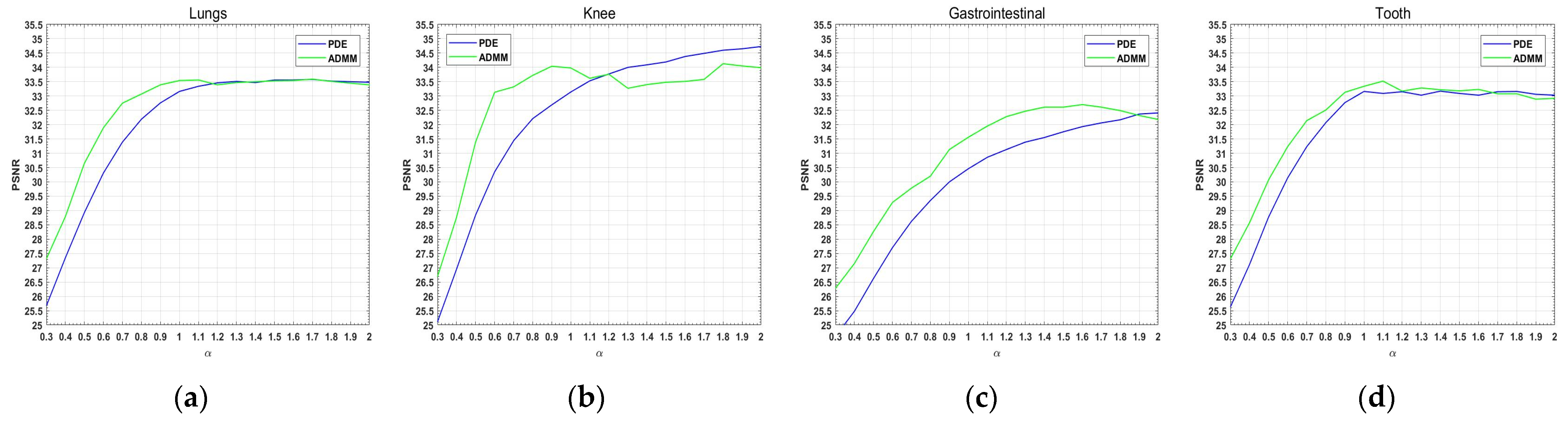
5.2.1. Experiments with Fractional Order $\mathsf{\alpha }$ and Regularization Parameter $\mathsf{\lambda }$

In this subsection, we test the sensitivity of a “Lungs” image (see Figure 2a) to fractional order $\alpha$ and regularization parameter $\lambda$ using the proposed model with the ADMM method. On the one hand, the balance between a good fit to the data and a regular solution using a regularization parameter $\lambda$ is difficult to determine in image restoration. On the other hand, since the fractional-order derivatives are nonlocal, the restoring effect will differ for different $\alpha$. As in the above experiments, we added Gaussian multiplicative noise with mean $1$ and variance $0.1$ to the “Lungs” image.

In Figure 3, (a) is a bar chart of the variation of PSNR and a line plot SSIM at different fractional order $\alpha$ when $\lambda =20$; (b) is a bar chart of the variation of PSNR and a line plot SSIM at different regularization parameter $\lambda$ when $\alpha =0.7$; and (c) is a plot of the variation of PSNR with respect to the order $\alpha$ and the parameter $\lambda$. From (a) and (b), we can find that the changes in PSNR values and SSIM values are consistent on the whole. From (a), we can see that PSNR and SSIM reach the maximum when $\alpha =1.7$. From (b), we can see that PSNR and SSIM reach the maximum when $\lambda =20$, and (c) shows that PSNR values are higher in the red region, which is consistent with our conclusions from (a) and (b). Thus, the optimal combination of $(\alpha ,\lambda )$ is $\left(\mathrm{1.7,20}\right)$ for the “Lungs” image. It also proves that the fractional-order model proposed in this paper is effective.

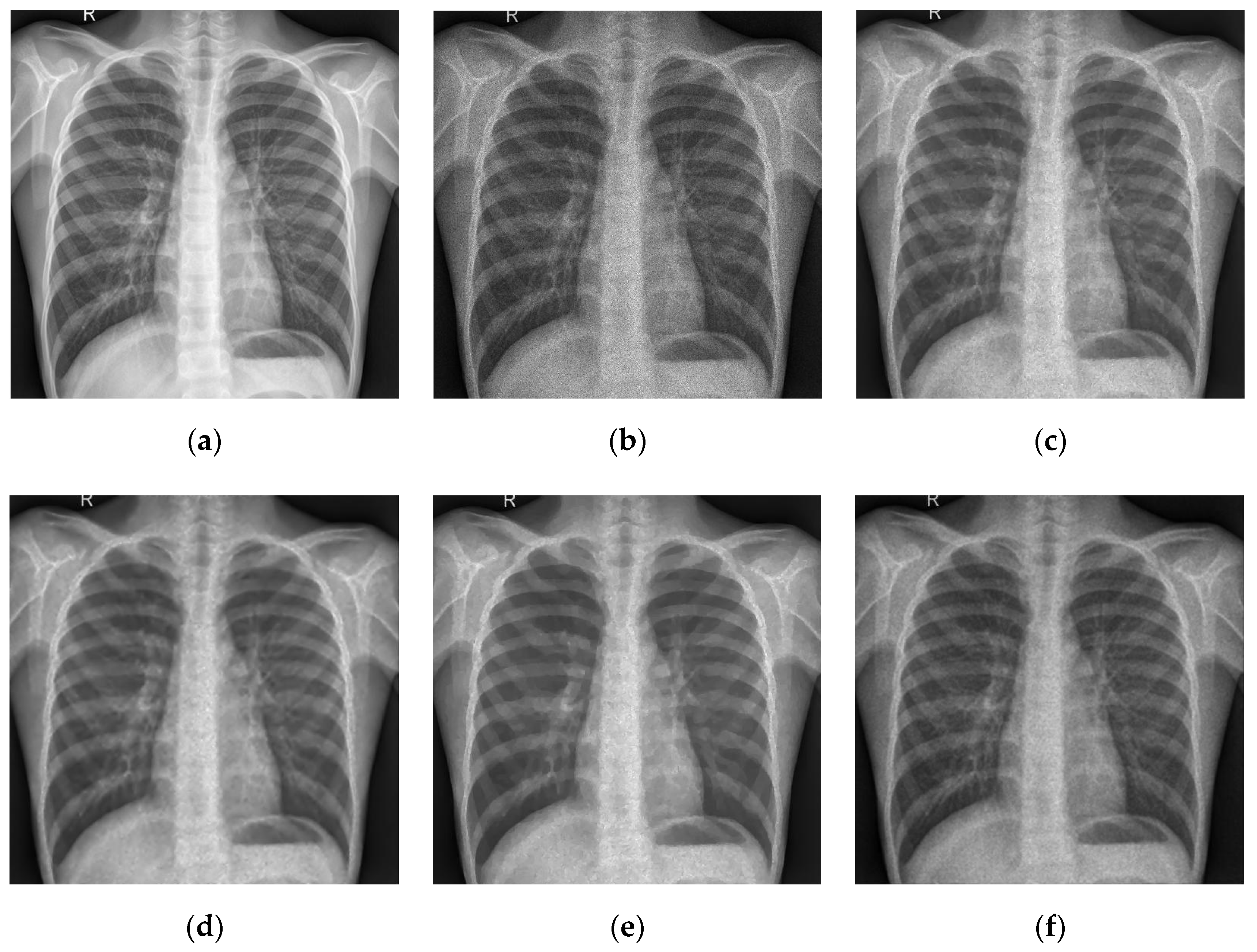
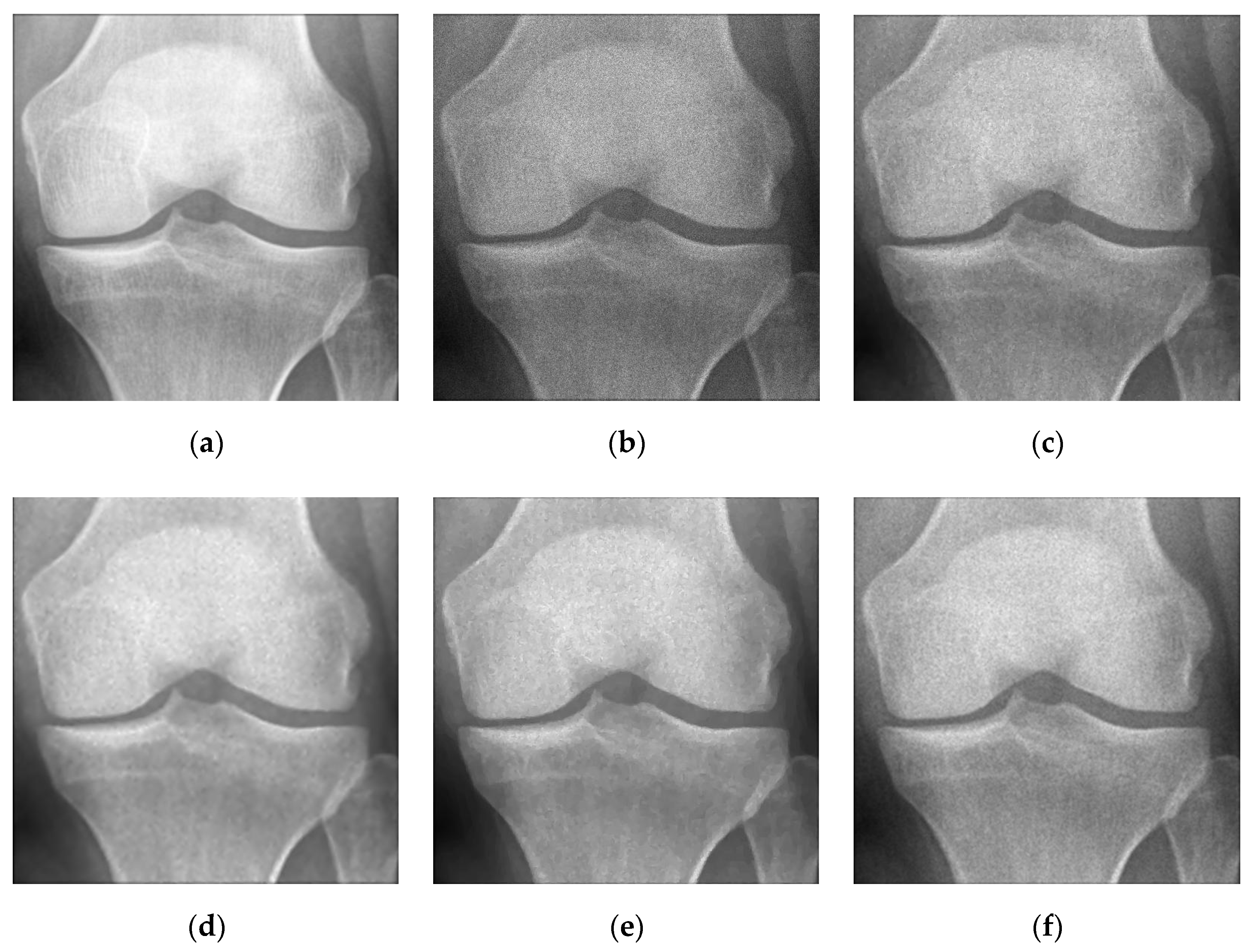
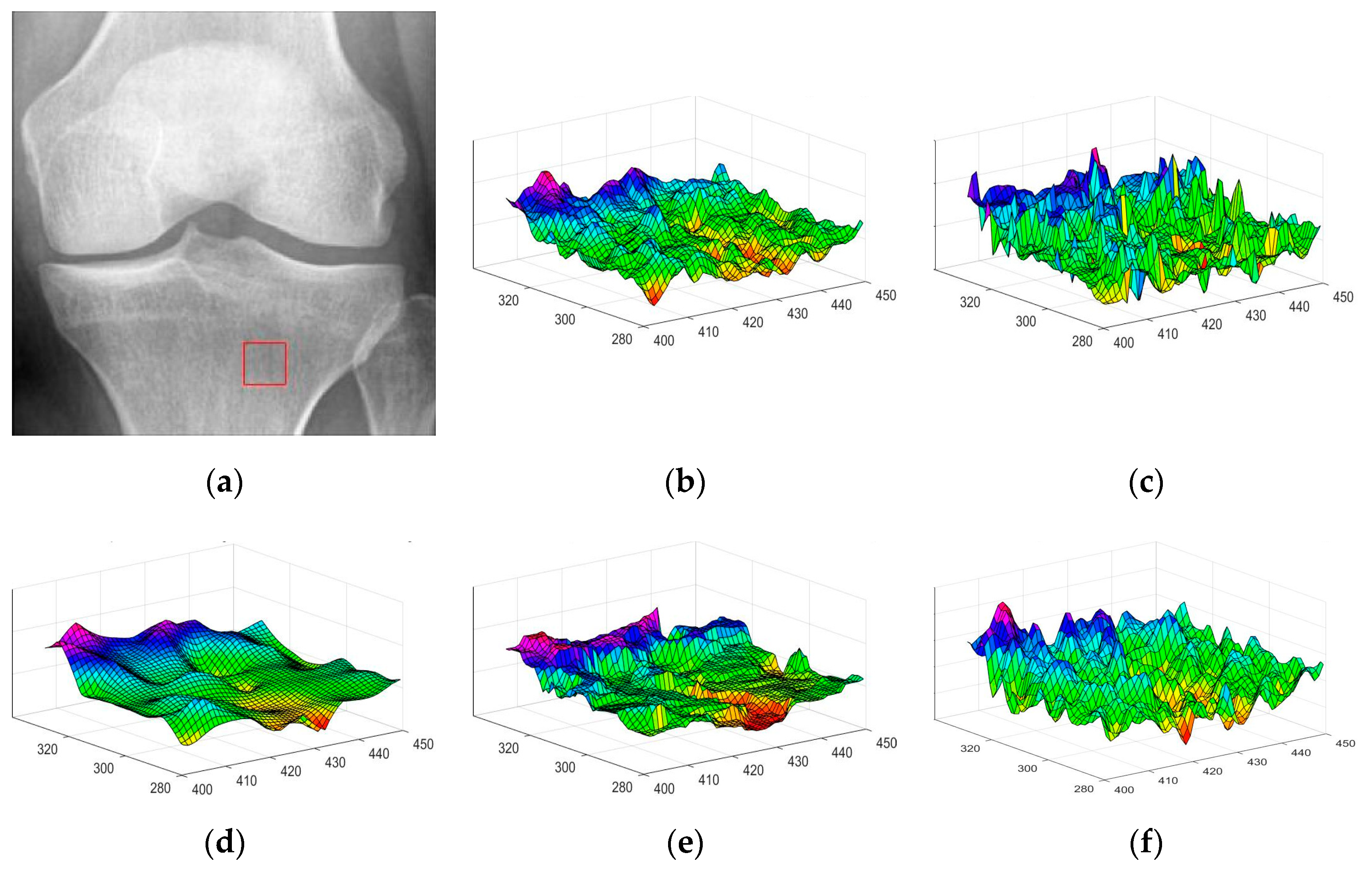
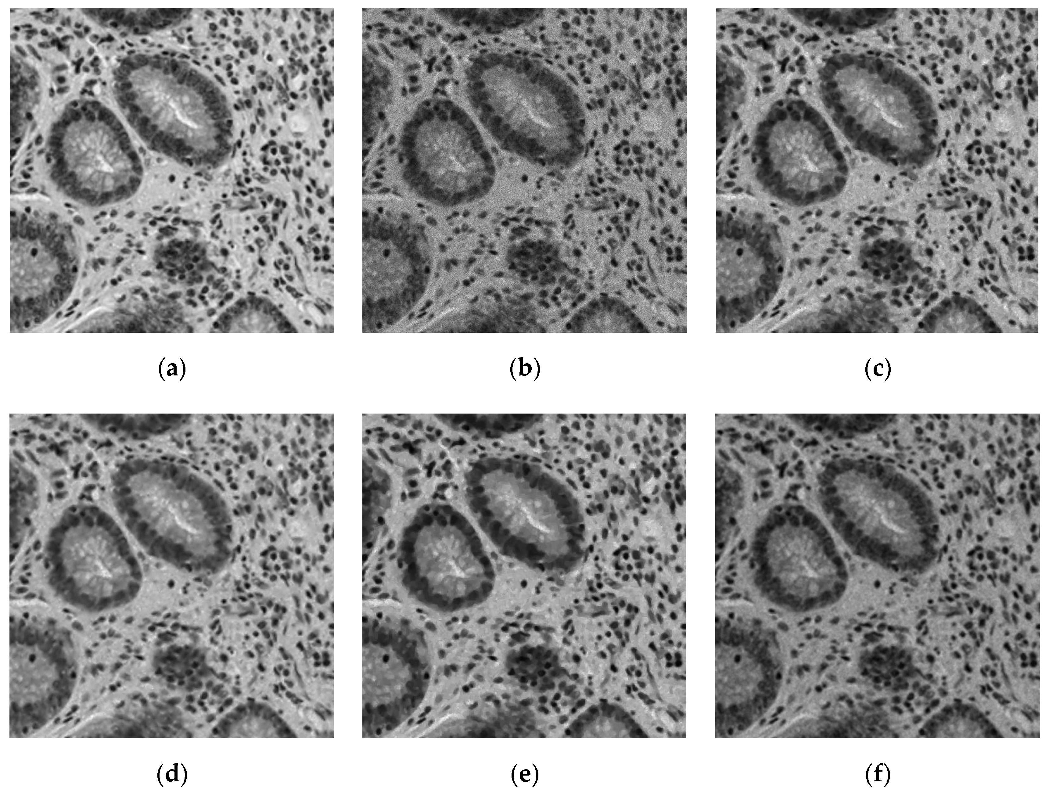
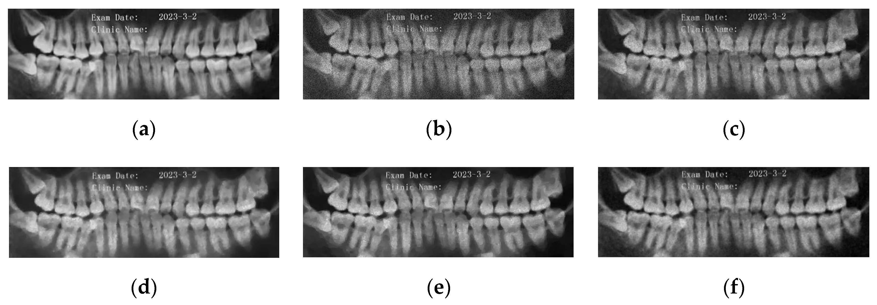
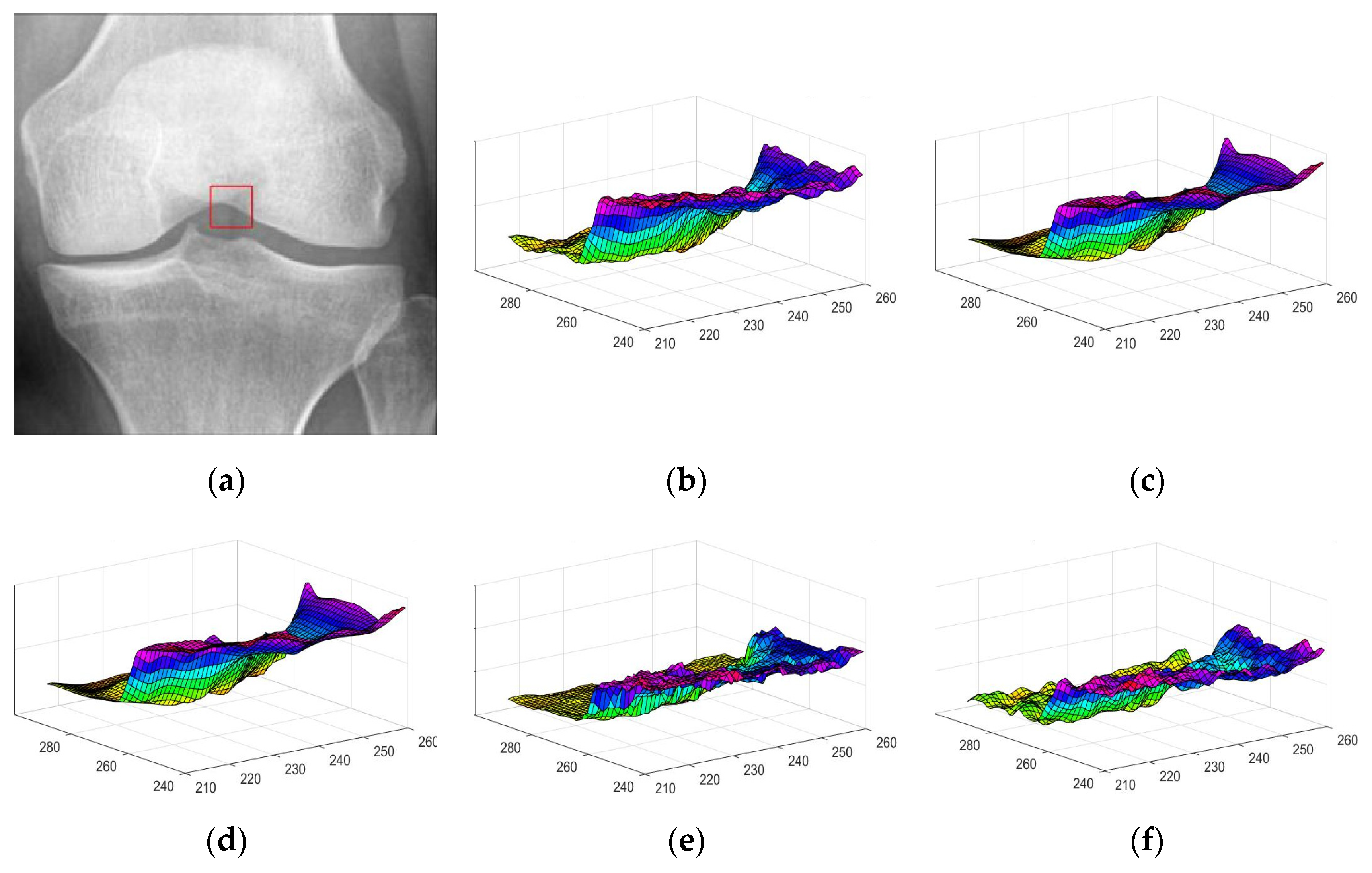
5.2.2. Different Methods

In this section, we utilize the partial differential equation method and the ADMM method to experiment on “Lungs”, “Knee”, “Gastrointestinal”, and “Tooth” images, as shown in Figure 2.

• Partial Differential Equation Method

In this experiment, we experimented with the four images in Figure 2 using the partial differential equation method. A Gaussian multiplicative noise level of $\mu =1,\sigma =0.1$ was added to the image. We chose $\mathsf{\alpha }$ values from $0.3$ to $2$ and $\lambda =0.05$ for the experiment. Figure 4 illustrates the PSNR value graphs of the four test images at different order $\mathsf{\alpha }$. The blue, red, yellow, and green lines represent “Lungs”, “Knee”, “Gastrointestinal”, and “Tooth”, respectively. From this we can see that the PSNR value basically increases as the order increases. Moreover, for “Knee’’ image, there is a larger magnitude of variation in the PSNR value, and the PSNR value is the largest after denoising.

• ADMM Method

Now, we add the same multiplicative Gaussian noise of $\mu =1,\sigma =0.1$ to the four images in Figure 2 and experiment with the ADMM method. In general, the magnitude of the value of parameter $\lambda$ is different for different test images, depending on the richness of the texture contained in the test image. For the image with more texture, the value of the parameter $\lambda$ should be lower than that for the image with less texture. Figure 5 shows the LBP texture extraction for the four test images. Here, we find that these four images have essentially the same texture richness, so they take the same value for the regularization parameter $\lambda$.

Figure 6 shows the original image, the noisy image, and the image after denoising using ADMM method at different orders (from $0.3$ to $2$), where the third and fourth rows represent their corresponding contour map. From this, it can be seen that when the order is too low, the recovered image still retains some of the noise. However, when the order is too high, the recovered image is excessively smooth. When the order is fractional order, the recovered image retains more texture details, which reduces the step effect compared to $\alpha =1$ and reduces the excessive smoothness compared to $\alpha =2$. As the order increases, the brightness of its recovered image is darker.

At the same time, we plot the PSNR values after denoising at different orders as line graphs in Figure 7. The horizontal axis represents the number of fractional orders, and the vertical axis represents the PSNR values. The blue, green, red, and purple colors represent the PSNR values of “Lungs”, “Knee”, “Gastrointestinal”, and “Tooth”, respectively. From the figure, it can be seen that as the order increases, the overall PSNR value increases and then decreases. In addition, the highest point basically does not occur at integer orders, and the practicality of the fractional order model proposed in this paper is therefore also demonstrated.

The PSNR values of denoised images under the partial differential equation method and ADMM method are shown in

Table 1. PSNR values obtained with different methods.

Images	Lungs		Knee		Gastrointestinal		Tooth
Fractional Orders	PDE	ADMM	PDE	ADMM	PDE	ADMM	PDE	ADMM
0.3	25.67	27.31	25.10	26.69	24.60	26.28	25.63	27.31
0.4	27.35	28.79	26.94	28.76	25.48	27.15	27.11	28.57
0.5	28.93	30.65	28.83	31.39	26.62	28.26	28.77	30.07
0.6	30.31	31.89	30.34	33.13	27.70	29.28	30.14	31.23
0.7	31.39	32.75	31.43	33.32	28.62	29.78	31.23	32.14
0.8	32.19	33.07	32.20	33.72	29.35	30.20	32.07	32.51
0.9	32.76	33.39	32.68	34.04	30.00	31.13	32.77	33.13
1.0	33.16	33.54	33.13	33.98	30.46	31.56	33.16	33.34
1.1	33.34	33.56	33.52	33.62	30.86	31.95	33.09	33.52
1.2	33.46	33.39	33.76	33.76	31.13	32.28	33.15	33.17
1.3	33.51	33.47	33.99	33.27	31.39	32.47	33.03	33.28
1.4	33.47	33.50	34.08	33.40	31.55	32.61	33.17	33.22
1.5	33.56	33.53	34.18	33.48	31.75	32.61	33.09	33.18
1.6	33.56	33.54	34.37	33.51	31.93	32.70	33.03	33.23
1.7	33.58	33.59	34.48	33.58	32.06	32.61	33.15	33.08
1.8	33.52	33.51	34.59	34.13	32.17	32.49	33.16	33.08
1.9	33.50	33.45	34.64	34.05	32.37	32.32	33.06	32.89
2.0	33.48	33.39	34.72	33.99	32.41	32.18	33.03	32.92

. Higher PSNR values are shown in bold. From the data in this table, it can be observed that in most of the cases the PSNR values after denoising using the ADMM method are higher than those obtained using the partial differential equation method for “Lungs”, “Gastrointestinal”, and “Tooth” images. However, for “Knee” images, at higher orders, the partial differential equation method gives better denoising results than the ADMM method.

In order to show the relationship between the PSNR values after denoising using the two methods more intuitively, we plot them using line graphs, as shown in Figure 8. From this figure, we find that both the PDE method and the ADMM method can effectively remove medical image noise. However, for symmetric and asymmetric images, their denoising results are not the same. For symmetric images, we find that the denoising results of the PDE method and the ADMM method are basically the same as the number of orders increases. However, for asymmetric images, as the number of orders increases, the denoising results of the PDE method are superior to those of the ADMM method. This also directly demonstrates that the model proposed in this paper is better at denoising images with symmetry.

5.2.3. Comparison with Other Variational Models

In this section, we compare the model proposed in this paper with already existing models, including the I-div model, the FI-div model, and the WI-div model. We determined the value of the fractional order $\alpha$ through qualitative assessment, quantitative assessment, and human physical psychology, and $\alpha$ values of $1.7, 1.8, 1.6,\mathrm{a}\mathrm{n}\mathrm{d} 1.1$ are chosen for “Lungs”, “Knee”, “Gastrointestinal”, and “Tooth” images, respectively.

First, we add Gaussian multiplicative noise with $\mu =1,\sigma =0.1$ to the test image in Figure 2, and the images obtained after denoising using the four models are shown in Figure 9, Figure 10, Figure 11 and Figure 12, where (a) is the original image, (b) is the noisy image, and (c–f) are the I-div, FI-div, WI-div, and our (FWI-div) denoised images, respectively. We find that the denoised image of the I-div model produces the step effect and contains a little noise, but it can better retain the edge information. The FI-div model can effectively reduce the step effect and retain more texture details. The WI-div model is subjectively better at denoising compared to the I-div model and the FI-div model, although it also has a step effect due to the fact that its regular term is low order like the I-div regular term. The model we propose in this paper not only retains the advantages of the FI-div model that can effectively avoid the step effect and retain more texture details, but also possesses the advantages of the WI-div model that is better from the supervisor’s visual effect. However, the recovered image is not as good as the other models in terms of luminance.

Next, we add Gaussian multiplicative noise with $\mu =1,\sigma =0.2$.

Table 2. PSNR and SSIM values at different noise levels.

σ = 0.1
	I-div		FI-div		WI-div		FWI-div
	PSNR	SSIM	PSNR	SSIM	PSNR	SSIM	PSNR	SSIM
Lungs	31.50	0.7876	33.98	0.8675	33.25	0.8437	33.59	0.8538
Knee	31.52	0.7319	36.04	0.9180	34.73	0.8589	34.73	0.8591
Gastrointestinal	29.92	0.8454	32.70	0.9163	30.72	0.8732	32.70	0.9165
Tooth	31.70	0.8384	33.38	0.8858	33.07	0.8979	33.52	0.8958
σ = 0.2
	I-div		FI-div		WI-div		FWI-div
	PSNR	SSIM	PSNR	SSIM	PSNR	SSIM	PSNR	SSIM
Lungs	23.31	0.4726	27.95	0.6953	25.57	0.5936	25.77	0.5978
Knee	22.60	0.3184	27.78	0.6246	25.01	0.4608	25.28	0.4694
Gastrointestinal	22.38	0.5700	26.82	0.7658	24.33	0.6573	24.98	0.6944
Tooth	23.62	0.4842	27.05	0.6992	26.10	0.6541	25.56	0.5784

shows the PSNR and SSIM values of different models after denoising at variance $0.1$ and $0.2$. In Table 2, we find that when the variance is $0.1$, our modeling method reaches the highest values for the “Gastrointestinal” and “Tooth” images. These values are not reached for the “Lungs” and “Knee” images, but the denoising effect is better than that obtained for both the I-div and WI-div models. At variance $0.2$, none of our models are the best. With the exception of the “Tooth” image, the PSNR values obtained after denoising using our model are higher than the PSNR values obtained after denoising with I-div and WI-div. This reflects that our model proposed in this paper is effective in removing slight noise to a certain extent, while its denoising effect is superior to that of the I-div and WI-div models when removing more severe noise. This also proves that our proposed model in this paper is effective to some extent.

In order to further investigate the recovery effect of the four models, we select two different rectangular regions of the “Knee” image and provide a three-dimensional surface map as shown in Figure 13 and Figure 14 after denoising by the four models. In both figures, (b) presents the three-dimensional surface map within the red rectangular region of the original image, and (c–f) are the three-dimensional surface maps in the red rectangular region after denoising using the I-div, FI-div, WI-div and our model, respectively. In Figure 13, the region noted in (a) is selected as a region with small gradient changes in the “Knee” image. In Figure 14, the region noted in (a) is selected for as a region with large gradient changes. From this, we find that I-div and WI-div can effectively preserve the edge information of the image, while FI-div and our model can effectively preserve the texture information of the image. From Figure 14, we find that the denoising effect of WI-div and our proposed model is not as good as that of I-div and FI-div models in places with large gradient variations, which indicates that the model combined with Weber’s model can better handle images with small gradient variations.

In conclusion, the model in this paper is the best of the four models in terms of quality and quantity in terms of texture preservation performance and visualization.

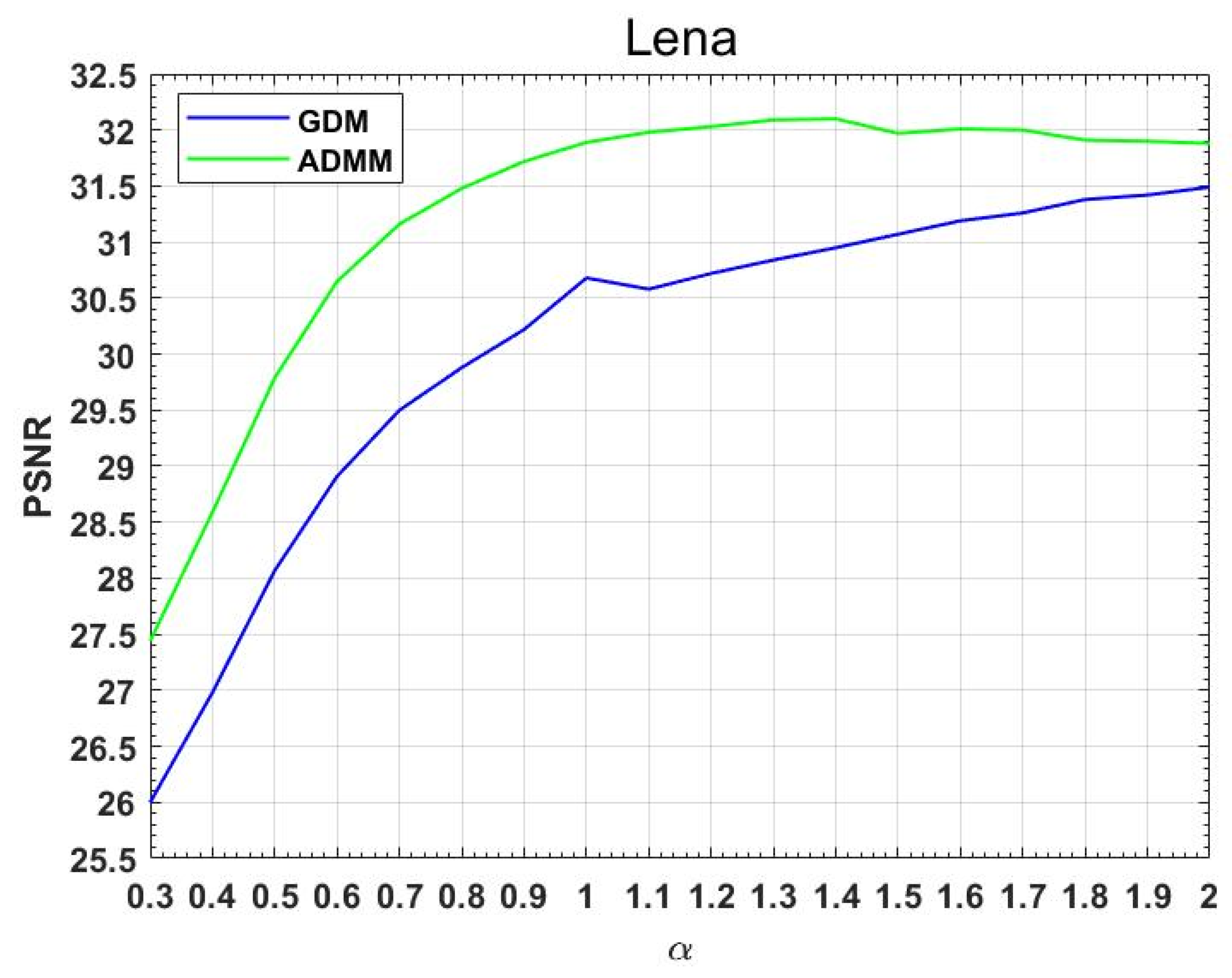
5.3. Numerical Simulations on Natural Image

In order to generalize the model proposed in this paper, Lena images are tested.

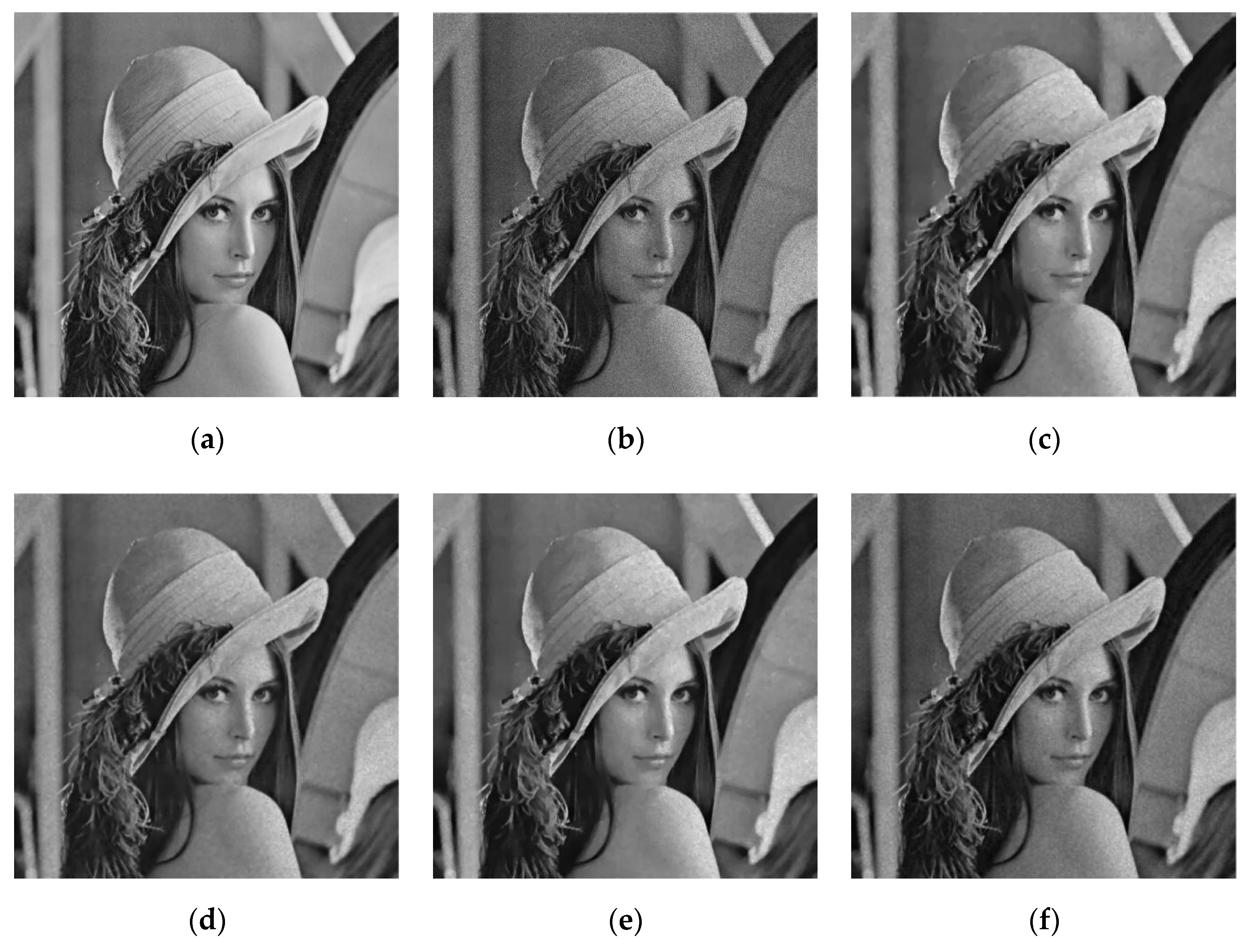
5.3.1. Different Methods

First, a Lena image with Gaussian multiplicative noise with a mean of $1$ and variance of $0.1$ is tested using the partial differential equation method and ADMM method.

In

Table 3. PSNR values for the Lena image obtained using different methods.

	PDE	ADMM
$\mathsf{\alpha }$	PSNR	PSNR
0.3	26.00	27.44
0.4	26.98	28.59
0.5	28.07	29.79
0.6	28.91	30.65
0.7	29.50	31.16
0.8	29.88	31.48
0.9	30.22	31.72
1.0	30.68	31.89
1.1	30.58	31.98
1.2	30.72	32.03
1.3	30.84	32.09
1.4	30.5	32.10
1.5	31.07	31.97
1.6	31.19	32.01
1.7	31.26	32.00
1.8	31.38	31.91
1.9	31.42	31.90
2.0	31.49	31.88

, the PSNR values of the Lena image after denoising using partial differential equation method and ADMM method are given, where the larger values are bolded. We find that the ADMM method is better than the partial differential equation method, which proves the effectiveness of the proposed algorithm. Figure 15 is a line chart of PSNR values obtained using the two methods. We find the above conclusions more directly. At the same time, we also find that the PSNR values obtained after denoising using the ADMM method present a trend of first increasing and then decreasing. The optimal PSNR value is not reached when $\alpha$ is an integer. However, when $\alpha =1.4$, the PSNR value is the largest. This also reflects that the fractional-order model proposed in this paper is reasonable and effective.

5.3.2. Comparison with Other Variational Models

Then, we add Gaussian multiplicative noise with $\mu =1,\sigma =0.1$ to the Lena image, and the images obtained after denoising using the four models are shown in Figure 16, where (a) is the original image, (b) is the noisy image, and (c–f) are the I-div, FI-div, WI-div, and FWI-div denoised images, respectively. We find that the denoised image of the I-div model produces the step effect and contains a little noise, but it can better retain the edge information. The model obtained using the Weber variational (WI-div) model has a better visual effect after denoising the image, while the fractional variational model (FI-div) retains more texture details to a certain extent. Our model (FWI-div) not only retains more texture details of the image but also improves the visual effect after denoising.

Table 4. PSNR and SSIM values obtained at different noise levels of the Lena image.

	σ = 0.1
	I-div		FI-div		WI-div		FWI-div
	PSNR	SSIM	PSNR	SSIM	PSNR	SSIM	PSNR	SSIM
Lena	32.38	0.8541	32.44	0.8547	32.21	0.8536	32.10	0.8259
	σ = 0.2
	I-div		FI-div		WI-div		FWI-div
	PSNR	SSIM	PSNR	SSIM	PSNR	SSIM	PSNR	SSIM
Lena	26.72	0.6329	28.12	0.7047	26.56	0.6344	28.59	0.7067

shows the PSNR and SSIM values of different models after denoising at $\sigma =0.1$ and $\sigma =0.2$. When $\sigma =0.1$, our model does not achieve the best results, but it is not different from other models. When $\sigma =0.02$, the denoising effect of the proposed model is the best. This shows that the model proposed in this paper has a better denoising effect for natural images with a high degree of noise.

In general, the model proposed in this paper can be applied not only to medical images but also to natural images, and the denoising effect of the model is effective to a certain extent.

6. Conclusions

In this paper, we propose a non-convex fractional-order denoising model for solving the image denoising problem contaminated by multiplicative noise using the definition of G-L fractional-order derivatives. The uniqueness of the existence of the solution of this model is proven, and we solve the proposed model using the partial differential equation (PDE) method and the alternating direction multiplier method (ADMM). Through extensive simulation experiments, numerical and visual results show that the ADMM method can be used to solve the non-convex multiplicative denoising model. In addition, the model proposed in this paper outperforms the other models (I-div, FI-div, WI-div) in terms of dimmer brightness; however, our recovered image is more realistic and natural. This motivates us to combine our model with integer-order models in our future work to further enhance the visual effect and improve the recovered PSNR values and to find other optimization algorithms that can be used to solve the non-convex model to use our proposed model for the restoration of medical images.

References

1. Rudin, L.; Lions, P.L.; Osher, S. Multiplicative Denoising and Deblurring: Theory and Algorithms. In Geometric Level Set Methods in Imaging, Vision, and Graphics; Springer: New York, NY, USA, 2003; pp. 103–119. [Google Scholar]
2. Liu, G.; Huang, T.Z.; Liu, J. High-order TVL1-based images restoration and spatially adapted regularization parameter selection. Comput. Math. Appl. 2014, 67, 2015–2026. [Google Scholar] [CrossRef]
3. Bioucas-Dias, J.M.; Figueiredo, M.A.T. Multiplicative Noise Removal Using Variable Splitting and Constrained Optimization. IEEE Trans. Image Process. 2009, 19, 1720–1730. [Google Scholar] [CrossRef]
4. Bioucas-Dias, J.M.; Figueiredo, M.A.T. Total variation restoration of speckled images using a split-bregman algorithm. In Proceedings of the 2009 16th IEEE International Conference on Image Processing (ICIP), Cairo, Egypt, 7–10 November 2009; pp. 3717–3720. [Google Scholar]
5. Teuber, T.; Lang, A. Nonlocal Filters for Removing Multiplicative Noise. In Proceedings of the Scale Space and Variational Methods in Computer Vision, Ein-Gedi, Israel, 29 May–2 June 2011. [Google Scholar]
6. Shama, M.G. Multiplicative noise removal using complementary total generalized variation and nonlocal low rank regularization. Optik 2023, 291, 171374. [Google Scholar] [CrossRef]
7. Lee, J.-S. Digital image enhancement and noise filtering by use of local statistics. IEEE Trans. Pattern Anal. Mach. Intell. 1980, 2, 165–168. [Google Scholar] [CrossRef]
8. Achim, A.; Bezerianos, A.; Tsakalides, P. Novel Bayesian multiscale method for speckle removal in medical ultrasound images. IEEE Trans. Med. Imaging 2001, 20, 772–783. [Google Scholar] [CrossRef] [PubMed]
9. Bai, J.; Feng, X.-C. Fractional-Order Anisotropic Diffusion for Image Denoising. IEEE Trans. Image Process. 2007, 16, 2492–2502. [Google Scholar] [CrossRef] [PubMed]
10. Zhang, J.; Wei, Z. A class of fractional-order multi-scale variational models and alternating projection algorithm for image denoising. Appl. Math. Model. 2011, 35, 2516–2528. [Google Scholar]
11. Chen, D.; Sun, S.; Zhang, C.; Chen, Y.; Xue, D. Fractional-order TV-l2 model for image denoising. Cent. Eur. J. Phys. 2013, 11, 1414–1422. [Google Scholar] [CrossRef]
12. Tian, D.; Xue, D.; Wang, D. A fractional-order adaptive regularization primal-dual algorithm for image denoising. Inf. Sci. 2015, 296, 147–159. [Google Scholar] [CrossRef]
13. Dong, F.; Chen, Y. A fractional-order derivative based variational framework for image denoising. Inverse Probl. Imaging 2016, 10, 27–50. [Google Scholar] [CrossRef]
14. Li, X.; Meng, X.; Xiong, B. A fractional variational image denoising model with two-component regularization terms. Appl. Math. Comput. 2022, 427, 12178–12192. [Google Scholar] [CrossRef]
15. Li, C.; He, C. Fractional-order diffusion coupled with integer-order diffusion for multiplicative noise removal. Comput. Math. Appl. 2023, 136, 34–43. [Google Scholar] [CrossRef]
16. Lian, W.; Liu, X. Non-convex fractional-order TV model for impulse noise removal. J. Comput. Appl. Math. 2022, 417, 114615. [Google Scholar] [CrossRef]
17. Weber, E.H. De Pulsu, Resorptione, Audita et Tactu, Annotationes Anatomicae et Physiologicae; Koehler: Leipzig, Germany, 1834. [Google Scholar]
18. Shen, J. On the foundations of vision modeling: I. Weber’s Law Weberized TV Restor. Phys. D Nonlinear Phenom. 2003, 175, 241–251. [Google Scholar] [CrossRef]
19. Xiao, L.; Huang, L.L.; Wei, Z.H. A weberized total variation regularization-based image multiplicative noise removal algorithm. EURASIP J. Adv. Signal Process. 2010, 2010, 490384. [Google Scholar] [CrossRef]
20. Yu, X.; Zhao, D. A Weberized Total Variance Regularization-based Image Multiplicative Noise Model. Image Anal. Stereol. 2023, 42, 65–76. [Google Scholar] [CrossRef]
21. Aubert, G.; Aujol, J.-F. A Variational Approach to Removing Multiplicative Noise. SIAM J. Appl. Math. 2008, 68, 925–946. Available online: https://www.jstor.org/stable/40233789 (accessed on 11 May 2023). [CrossRef]
22. Shi, J.; Osher, S. A nonlinear inverse scale space method for a convex multiplicative noise model. SIAM J. Imaging Sci. 2008, 1, 294–321. [Google Scholar] [CrossRef]
23. Steifdl, G.; Teuber, T. Removing Multiplicative Noise by Douglas-Rachford Splitting Methods. J. Math. Imaging Vis. 2010, 36, 168–184. [Google Scholar] [CrossRef]
24. Powell, M.J.D. A Method for Nonlinear Constraints in Minimization Problems; Academic Press: New York, NY, USA, 1969. [Google Scholar]
25. Boyd, S.; Parikh, N.; Chu, E.; Peleato, B.; Eckstein, J. Distributed Optimization and Statistical Learning via the Alternating Direction Method of Multipliers. Now 2011, 3, 1–22. [Google Scholar] [CrossRef]
26. Cai, J.-F.; Osher, S.; Shen, Z. Split Bregman Methods and Frame Based Image Restoration. Multiscale Model. Simul. 2009, 8, 337–369. [Google Scholar] [CrossRef]
27. Chan, S.H.; Wang, X.; Elgendy, O.A. Plug-and-Play ADMM for Image Restoration: Fixed-Point Convergence and Applications. IEEE Trans. Comput. Imaging 2016, 3, 84–98. [Google Scholar] [CrossRef]
28. Shapiro, J.M. Embedded image coding using zerotrees of wavelet coefficients. IEEE Trans. Signal Process. 1993, 41, 3445–3462. [Google Scholar] [CrossRef]
29. Giusti, E. Minimal Surfaces and Functions of Bounded Variation; Springer Science and Business Media LLC: Dordrecht, The Netherlands, 1984. [Google Scholar]
30. Aubert, G.; Kornprobst, P. Mathematical Problems in Image Processing: Partial Difierential Equations and the Calculus of Variations; Springer: Berlin/Heidelberg, Germany, 2006; p. 147. [Google Scholar]
Figure 1. Amplitude–frequency characteristic curves for each order of differentiation.
Symmetry 16 00258 g001
Figure 2. Four Test Images. (a) Lungs. (b) Knee. (c) Gastrointestinal. (d) Tooth.
Symmetry 16 00258 g002
Figure 3. Sensitivity tests for fractional order α and regularization parameter λ . (a) is the change in fractional order; (b) is the change in the regularization parameter; (c) is the change in fractional order and the regularization parameter.
Symmetry 16 00258 g003
Figure 4. Variation of PSNR values under the PDE method.
Symmetry 16 00258 g004
Figure 5. Texture map of the test image. (a) LBP of “Lungs.” (b) LBP of “Knee.” (c) LBP of “Gastrointestinal.” (d) LBP of “Tooth”.
Symmetry 16 00258 g005
Figure 6. The original, noisy, and denoised images (ADMM).
Symmetry 16 00258 g006aSymmetry 16 00258 g006b
Figure 7. Changes in PSNR values for different orders under the ADMM method.
Symmetry 16 00258 g007
Figure 8. Comparison of PSNR for ADMM and PDE. (a) Lungs. (b) Knee. (c) Gastrointestinal. (d) Tooth.
Symmetry 16 00258 g008
Figure 9. Comparison of the four models on the “Lungs” image. (a) original image (b) noisy image (c) I-div denoised image (d) FI-div denoised image (e) WI-div denoised image (f) our denoised image.
Symmetry 16 00258 g009
Figure 10. Comparison of the four models on the “Knee” image. (a) original image (b) noisy image (c) I-div denoised image (d) FI-div denoised image (e) WI-div denoised image (f) our denoised image.
Symmetry 16 00258 g010
Figure 11. Comparison of the four models on the “Gastrointestinal” image. (a) original image (b) noisy image (c) I-div denoised image (d) FI-div denoised image (e) WI-div denoised image (f) our denoised image.
Symmetry 16 00258 g011
Figure 12. Comparison of the four models on the “Tooth” image. (a) original image (b) noisy image (c) I-div denoised image (d) FI-div denoised image (e) WI-div denoised image (f) our denoised image.
Symmetry 16 00258 g012
Figure 13. The three-dimensional surface maps produced by the four models for the “Knee” image with small gradient changes. (a) Original image with red rectangular region (b) the three-dimensional surface map within the red rectangular region of the original image (c) the three-dimensional surface map in the red rectangular region after denoising using the I-div model (d) the three-dimensional surface map in the red rectangular region after denoising using the FI-div model (e) the three-dimensional surface map in the red rectangular region after denoising using the WI-div model (f) the three-dimensional surface map in the red rectangular region after denoising using our model.
Symmetry 16 00258 g013
Figure 14. The three-dimensional surface maps produced by the four models for the “Knee” image with large gradient changes. (a) Original image with red rectangular region (b) the three-dimensional surface map within the red rectangular region of the original image (c) the three-dimensional surface map in the red rectangular region after denoising using the I-div model (d) the three-dimensional surface map in the red rectangular region after denoising using the FI-div model (e) the three-dimensional surface map in the red rectangular region after denoising using the WI-div model (f) the three-dimensional surface map in the red rectangular region after denoising using our model.
Symmetry 16 00258 g014
Figure 15. Comparison of PSNR values obtained using ADMM and PDE on the Lena image.
Symmetry 16 00258 g015
Figure 16. Comparison of the four models using the Lena image. (a) the original image (b) the noisy image (c) the I-div denoised image (d) the FI-div denoised image (e) the WI-div denoised image (f) ours denoised image.
Symmetry 16 00258 g016