1. Introduction
Batteries are electrochemical devices used for storing energy generated using a cell packaged with a cathode and an anode submerged in an electrolytic solution [
1,
2,
3,
4,
5,
6,
7,
8,
9,
10,
11,
12]. Lead and sulfuric acid are in vehicle batteries; these are the most popular product where lead is. Nevertheless, the components are toxic and corrosive, can pollute air, soil, and water, and can also be cause for an explosion or a fire. Moreover, exposure to these components can produce serious health hazards to humans and natural life [
1,
2,
3,
7,
13,
14,
15,
16,
17,
18,
19,
20]. Zhang, li Sun, and other authors have talked about some industrial methods for recycling hazardous materials. Although lead–acid batteries can be physically recharged many times, their working life is limited, as during each cycle, certain stress is placed on the lead plates, according to the operating conditions [
3,
4,
6,
7,
9,
10,
11,
12,
13]. This causes short circuits and reduces the battery’s lifetime [
2,
3,
4,
5,
13]. Prengaman, Hildebrandt, and Tian et al. have been working also on the recycling of lead batteries due to the fact that these are one of the most dangerous wastes in the automotive industry [
5,
6,
7,
8,
12,
16,
17,
18,
19].
Industrially, lead is collected for recycling and reducing environmental damage. Furthermore, the recycling process uses less energy than refining primary ore [
2,
3,
4,
5,
6,
7,
8,
13,
14]. Nowadays, recycling has become a clean economical option for many industrial trials which want to reduce costs; this fact is a very interesting motivation for studying and improving industrial lead processing [
1,
2,
3,
4,
6,
7,
8,
9,
14,
15]. Furthermore, the evaluation of mixing performance is very important for reducing working times and increasing stirring efficiency. That is the reason why this work can be considered as an initial approach to establish mathematical parameters to evaluate industrial practices and improve the actual procedures [
6,
7,
8,
14,
15].
Some authors have been working on the simulation of fluid flows involving lead recycling inside chemical reactors [
10,
11,
12,
19,
20,
21,
22,
23]. But the geometrical configuration of reactors and the operating conditions are different for each industrial case, making stirring in chemical reactors a complex problem [
5,
6,
7,
8,
14,
15,
20,
21,
22,
23,
24,
25,
26,
27]. Some of these authors have been working with computer simulations showing concentration profiles as evidence of mixing or making physical models to compare results. Other authors like Debangshu have worked on suspensions of solids in recycling procedures, and Feng Wang has studied the measurement of phase holdups in stirred tanks [
9,
10,
20,
21,
22,
23,
24,
25,
26,
27]. But the simulation of stirring inside a tank is a complex problem where many variables are involved in terms of the Navier–Stokes equations, and many phenomena must be solved to understand hydrodynamics. Some authors have been testing this by inducing turbulence effects on solid–liquid suspensions to solve problems related to polymerization [
20,
21,
22,
23]. Rahimi, Lassin, and others studied hollow impeller effects to validate experimental fluid dynamics using CFD in order to evaluate the influence of the impeller speed [
28,
29,
30]. Some authors simulated lead bullion in hemispherical vessels known as kettles [
9,
10,
11,
12,
14,
15,
31,
32,
33,
34]. Other authors have studied fluid flow dynamics in reactors for different purposes, such as the analysis of resin beads and ways of scaling up. But hydrodynamic behavior and physical properties are particular for each simulated case [
10,
11,
12,
14,
16,
17,
18,
19]. These authors have provided important knowledge for understanding the hydrodynamic behavior of fluid in chemical reactors. Other authors have studied the effect of perturbations in stirred tanks [
19,
20,
21,
22,
23,
24,
25,
30,
35,
36,
37,
38]. Others have been analyzing chemical reactions and the evolution of liquid–liquid phases [
17,
18,
19,
20,
21,
22,
23,
26,
27,
28,
29,
36,
37,
38,
39,
40]. Murthy, Zhong Zhang, Sossa-Echeverria, Szalai, and others have dedicated their works to evidencing the influence of tanks and impeller geometries [
16,
17,
18,
19,
20,
21,
22,
23,
35,
36]. Some of them have used the residence time distribution method to analyze efficiency in a stirred tank [
12,
15,
26,
27,
28,
29,
30,
31,
32,
33,
34,
41,
42,
43]. Others have simulated dissolutions in tanks and validated these procedures as appropriate for establishing physical parameters to improve mixing [
11,
12,
16,
17,
18,
19,
20,
21,
22,
23,
24,
25,
26,
27,
28,
29]. In 2016, Divyamaan worked on a computer simulation of solid–liquid stirred tanks. Tamburini et al. have produced similar works considering solid–liquid suspension and predicting the solid particle distribution and the minimum impeller speed for homogeneous mixing. To conclude, an understanding of the hydrodynamics phenomena involved is very important to improve actual industrial practices in many metallurgical processes [
17,
18,
19,
20,
21,
22,
23,
24,
25,
26,
27,
28,
29,
30,
35,
36,
39,
40,
41,
42,
44,
45,
46,
47,
48,
49]. Some authors have been studying problems of phenomena related to fluids confined in industrial tanks such as the solid suspension of particles involving chemical reactions evaluating fluid hydrodynamics behaviors under symmetrical and asymmetrical jet conditions [
32,
33,
34,
36,
37,
38,
39,
40,
43,
44,
45,
50,
51,
52]. Authors have also been developing numerical methods and new approaching techniques for fluid evaluation [
6,
7,
8,
14,
15,
31,
32,
33,
34,
42,
43,
50], inclusively, other metallurgical problems where pyro-processing and the hydrodynamics of liquid metals can be analyzed to improve industrial practices [
11,
12,
16,
17,
18,
26,
27,
28,
29,
31,
32,
33,
34,
41,
42,
43].
2. Geometrical Model (Tank Reactor and Impeller)
As was commented previously, there are many aspects influencing the mixing process in chemical batch reactors: the geometry of the batch, impeller mechanisms, industrial working conditions, and properties of the fluids and phases. Moreover, the considerations that are selected, like the use of laminar conditions or the inclusion of mathematical turbulence models, can affect results. Then, in the present work, the geometrical configuration of the reactor was built computationally based on real industrial data. A simulation of the hydrodynamics fluid flow is performed using the software Fluent (6.0), and the results of the tracer concentration on each monitoring node are saved at every time step (
t + Δ
t) on independent files to be analyzed using Microsoft Excel in order to evaluate the mixing efficiency [
9,
10,
14,
15,
25,
26,
27,
28,
29]. These values are compared with tracer concentration profiles in order to find zones with good or poor mixing and its contribution to the entire homogeneity.
The industrial reactor analyzed consists of two parts. The first is the main upper body with a cylindrical form and the second is a semispherical section on the bottom, as shown in
Figure 1. The cylindrical diameter is 0.44 m, and the cylinder is 0.470 m high. The reactor is symmetrical along the vertical and horizontal axes. Then, a triangular mesh using two-dimensional elements which form a surface model is defined for the walls discretization, since it is only necessary to declare the surface of the reactor walls as a closed boundary [
7,
8,
9,
10,
11,
14,
15,
25,
41,
42,
48,
49]. These walls are also declared free of defects and friction. The mesh used for discretization is not structured with 1062 cells and a regular size. The two sections were traced assuming the center on the cylindrical section at the lowest position and the top center of the semispherical bottom. This intersection point is taken for reference as the origin for the tank (0, 0, 0). Then, we defined two original planes which were joined forming only one single surface that cuts the batch reactor symmetrically.
The areas measured of the cylindrical and semispherical sections are 0.66922116 m2 and 0.282244 m2, respectively, forming a solid wall with 0.9514656 m2. A non-structured mesh with triangular cells was selected for a good fit with the cylindrical and semispherical regions of the reactor.
The industrial reactor was stirred using one single impeller formed with a vertical shaft and two rectangular flat solid blades joined in the low shaft position, as can be appreciated in
Figure 2a,b. The shaft is 0.610 m in length: enough to be placed inside the reactor, and the four rectangular blades (0.0508 m × 0.0254 m) are form from the intersection of the two flat solids. These blades are placed symmetrically (each 90°) and are 0.00375 m thick. Here, a mesh with triangular 2D and tetragonal 3D cells is used again for the discretization of the entire element surface. The shaft is discretized using 16,890 two-dimensional cells, 657 two-dimensional cells are used for each impeller blade, and the measured area for the shaft is 0.1476181 m
2.
The lead bulk volume inside the reactor is obtained applying an inverse negative geometrical Boolean operation. The volume results from the original volume between the walls minus the impeller volume, which was discretized using 22,097 nodes forming 210,235 two-dimensional cells (triangular), which forms 99,923 tri-dimensional cells (tetrahedral). To obtain a good approach, the smallest cell elements were placed near the impeller, and the biggest cells were placed near the wall reactor, since the contact with the impeller for the fluid movement simulation is very important. Moreover, the volume of the tank obtained is the volume of liquid lead simulated.
Additionally, the tank reactor was modeled using different types of meshes, as is shown in the validation section and also was compared with a basic physical model.
3. Semi-Planes, Injection and Monitoring Points, and Initial Assumptions
The reactor is symmetrical vertically; here, a control plane is taken for reference purposes, as shown in
Figure 3 and
Figure 4. The control plane was divided into two semi-planes. The first of them was the injection plane. Here, all the nodes where the tracer would be injected for each simulation were indicated. All of these were evaluated independently in order to find the best injection point. The second plane was the monitoring plane. Here, we placed the points where the mixing efficiency would be measured and evaluated. The position of every point of both planes is shown in
Table 1 and
Table 2, respectively.
The injection points were placed on different places to know their position influence on the injection semi-plane and evaluate the changes on the hydrodynamic behavior with a common reactor geometry and impeller during specific rotatory conditions, enabling identifying death zones (zones with poor mixing) and zones with delays in mixing. The points (Pi1, Pi4, Pi8, Pi14, and Pi18) are placed along the shaft from the reactor surface to the blades. The nearest injection points to the wall are Pi6, Pi12, Pi16, Pi21, and Pi22. The points in the middle tank position are Pi2, Pi3, Pi5, Pi7, Pi10, Pi13, Pi15, and Pi17. Finally, only one single point was placed on the bottom for evaluating hydrodynamic behavior in this zone (Pi20). Here, the sub-index “i” is used to indicate the injection point.
The parameter to evaluate mixing efficiency inside the entire reactor is the tracer distribution. This was conducted by measuring it on each monitoring point. The monitoring points were also placed all around the semi-plane to measure the tracer concentration in different zones inside the tank. The purpose is to identify zones with rich and poor mixing and relate them with the hydrodynamic behavior and the evolution of tracer dispersion. The monitoring points were placed on the monitoring semi-plane at 180° from the injection semi-plane, as shown in
Figure 4. These points were used for saving the tracer concentration (C
m) at every time step (
t + Δ
t) during the simulation. Here, the sub-index “m” is used to indicate the monitoring points. Initially, for
t = 0, it is assumed the tracer concentration on each monitoring point is equal to zero (C
m = 0). Some of these points were placed in the middle of the reactor such as Pm
2, Pm
7 and Pm
12; some others were placed near the walls such as Pm
03 to Pm
06 and Pm
08 to Pm
11. Finally, the rest of these were placed at the bottom such as Pm
13, Pm
14 and Pm
15. Here, evaluation is very important because this region is critical for mixing.
4. Assumptions
The following assumptions and boundary conditions are taken into account for all the simulations exposed in this work:
The impeller shaft is in the middle position of the reactor body for symmetrical conditions. Additionally, no vibration is assumed during rotation; then, the influence of the shaft rotation is not significant. Consequently, the only elements that provide stirring to the bath are the four blades.
Rugosity on tank walls (cylinder and semispherical) is neglected as a consequence of the fluid displacement being free, and no drag is induced.
The impeller rotates at 200 radians per minute: approximately 32 RPMs.
The surface of the liquid lead is flat; this condition is equivalent to assuming a closed reactor on the tank top. The lead surface is discretized with 1512 two-dimensional cells, and the measured area is 0.149812 m2.
The maximum face area for a cell used for discretization is 1.9733 × 10⁻³ m2 in contrast the minimum cell face area is 2.0324 × 10⁻⁶ m2.
The temperature of liquid lead is assumed as 327.46 °C (equal to 600.61 K or 621.43 F). This is the lead melting point, and the lead density equal to 10.66 g/cm3. Then, liquid lead is a heavy incompressible fluid.
During all analyzed cases on simulations, no heat interchange is assumed (isothermal system); then, the lead properties remain constant.
The tank is considered as isolated, there is no mass interchange, the volume is constant inside, and the tracer replaces a defined lead volume in the 3D mesh.
The movement of fluid is not a step pulse defined and not a continuous injection; the tracer volume replaced is moved as a consequence of the inertial forces due to the impeller impulse.
The time step (Δt) used for simulation was 5.208 × 10⁻³ and represents a rotation of 1° around the tank circumference considering the rotatory speed of the impeller.
There is no volume or mass interchange during the simulation; moreover, the movement of the fluid is due exclusively to the inertial forces of the velocity generated by the impeller movement.
The tracer takes place (is injected computationally) inside the tank reactor when the velocity of the fluid is stable. Then, this is considered as the beginning of the simulation cases. The distribution of the velocity vectors due to the impeller rotation can be appreciated in
Figure 5a–c; here, the biggest vectors can be appreciated near the blades, and the smallest vectors are in the tank body. During experimental mixing operations, a tracer can be injected using a tubing inlet system submerged into the bath. Nevertheless, this is not performed in the present work. The tracer cannot be injected computationally. The simulation is performed by replacing a defined lead volume, which is 125 cm
3 = 1.25 × 10
−4 m
3. Then, the tracer distribution is saved and evaluated dynamically as simulations run. During every simulation, only one single lead volume is replaced on the injection cells by an identical tracer volume at the beginning of the simulation (
t = 0). Consequently, the tracer is assumed as ideal; then, an original lead volume is substituted by another volume with the same physical properties. This method is frequently used by authors who work on physical and computer simulation to evaluate fluid flows [
1,
2,
3,
4,
5,
10,
11,
12,
13,
16,
17,
18,
30,
35,
36,
37,
38,
39,
40]. This procedure is conducted experimentally using colorants for painting the original fluid in order to follow the fluid path and show streamlines of fluid [
5,
6,
7,
13,
26,
27,
28,
29,
30,
39,
40,
44,
45,
46]. Nevertheless, in real industrial practices, solid chemicals for cleaning lead are incorporated to the bath tank using a lance inside. The lance can be placed at different positions in the cylindrical body; but, geometrically, it is complicated to inject below the impeller.
5. Mathematical Modeling
The equations solved on the mathematical model are given by Navier–Stokes and continuity. The Navier–Stokes equations describe the motion of fluids. These equations arise from applying Newton’s second law [
10,
11,
12,
16,
17,
18,
24,
25,
26,
27,
28,
29,
30,
35,
36]. The Navier–Stokes equations are nonlinear partial differential equations in almost every real situation. In some cases, such as one-dimensional flow, these equations can be simplified to linear equations. Nevertheless, nonlinearity carries most problems that are difficult or impossible to solve with conventional analysis because the main contributor is turbulence [
9,
10,
11,
12,
16,
26,
27,
28,
29,
30,
35,
36,
37,
38]. The numerical solution of the Navier–Stokes equations for turbulent flows is complex due to the significantly different mixing length involved in turbulent flow. Then, the stable solution of these equations requires the definition of a fine mesh during discretization to make the computational treatment of data feasible [
5,
23,
24,
25,
26,
27,
28,
29,
36,
37,
38,
39]. Turbulence models such as the k-ε model are used in practical computational fluid dynamics (CFD) applications where turbulent flows are modeled as is shown in this work [
32,
33,
34,
35,
36,
37,
38,
39]. The Navier–Stokes equations are strictly a statement of the conservation of momentum laws. Thus, in order to describe fluid flow, more information is required according to particular geometrical case data and including particular boundary conditions. Moreover, the basic concepts involved are the conservation of mass and the conservation of energy related to an equation of state [
30,
35,
36,
37,
38,
45,
46,
47,
48]. All these must be appropriately established. Then, a statement of the conservation of mass is achieved through the mass continuity equation, as shown in Equation (1).
Then, Navier–Stokes equations can be solved in three coordinate systems; here, Cartesian is the system solved and equations are taken directly from the vector equations [
36,
37,
38,
39,
40]. The solution implies the programming of Equations (2)–(4) using an explicit numerical method. Here, the velocity components are typically named
u,
v, and
w, which are the dependent variables to be solved.
Note that gravity was assumed as a body force, and the values of
gx,
gy, and
gz will depend on the orientation of gravity with respect to the chosen set of coordinates; for the reactor analyzed,
gx and
gy will be equal to zero; and only
gz participates in the fluid motion. Then, the continuity equation can be written as follows:
When the flow is at a steady state, (ρ) does not change with respect to time. Instead, the continuity equation can be simplified to:
When the flow is incompressible, ρ is constant and does not change with respect to space or time, and the continuity equation is reduced again to:
The partial differential equation for the mass transfer (equation of continuity) can be written in rectangular coordinates as is shown in Equation (8) and in cylindrical and spherical coordinates as shown in Equations (9) and (10), respectively, representing a solution for the Fick’s law equation; these equations can be solved for regular structured or non-structures and hexahedral or tetragonal or any other cells incorporated in nested loops and using a finite element method. Here, the k-ε model is used to solve the problem including turbulence; then, tracer concentration values over monitoring points are stored after every time step (p
mt+Δt); finally, data are analyzed using Microsoft Excel. It is important to mention that the tank with a mix of lead + tracer can be considered as a multicomponent fluid problem, as represented in Equation (11) [
42]. Here,
Deff is the diffusion and turbulent coefficient.
6. Computer Simulations
The model used for simulation was (k-ε), and the software used for solving was Fluent 6.0; hydrodynamic behavior is studied calculating and saving the tracer concentration at each step (
t + Δ
t) during simulations on every monitoring point.
Figure 6a–c show the tracer concentration on all the monitoring points for the injection points Pi
11, Pi
18, and Pi
21, respectively. These monitoring points were placed inside the tank, near and far from the impeller. Some of the curves in these figures show parabolic behavior and others are sinusoidal. Sinusoidal curves are near the impeller; here, the tracer concentration changed at every time step during simulation due to the strong influence of turbulence and vector velocities. In contrast, parabolic behavior is frequently observed near the walls and at the bottom of the tank, where the homogenization of tracer concentration is very slow, and no strong fluctuations are presented because these points are far away from the impeller influence. The tracer begins to be distributed by stirring from values equal to zero (the tracer is absent on monitoring points). Then, as the simulation time advances, there are some periods when the tracer concentration is increased and others when it is decreased. Nevertheless, these fluctuations are reduced as the simulation continues. The reduction on this fluctuation is considered as a parameter to evaluate mixing. Thus, for long times, all the monitoring points tend to adopt the same averaged concentration. This means that the tracer has been homogeneously distributed. There are curves with high tracer saturations on
Figure 6a,c; this is not good for mixing; these excesses must be stirred to obtain a homogeneous distribution.
Figure 6a shows that only a few curves are parabolic and remain always with a low tracer concentration. Nevertheless, these curves take a lot of time to reach the final average concentration, indicating poor mixing in these regions. Thus, according to the time scales in the horizontal axes, it is possible to appreciate that the best injection point is Pi
18; here, the tank delay is only 450 s. On the other hand, the worst injection point is Pi
21 with delays of more than 1400 s, and the tracer distribution injecting on Pi
11 is considered as an intermediate behavior.
In
Figure 6b, only one curve presents a high tracer concentration, and others have minor excesses. This means that minor stirring work must be applied for mixing.
Figure 6c shows there are some curves with high tracer concentrations, but there are also many curves with a very poor concentration which are located near the bottom, because accessing this zone is very difficult. Moreover, all curves tend to the same the final value; this variability is considered as homogeneity criterion for the mixing. Thus, finding the best injection point is the first way to improve industrial practices. In
Figure 6a–c, similar behavior can be appreciated on the corresponded monitoring points for every different injection point; nevertheless, curves are affected by the analyzed injection point.
Tracer concentration on all the monitoring points can be stored and then averaged to obtain a significant value of the tracer concentration inside the reactor which represents the entire behavior. Equation (12) can be used to represent this process; here, the sum in the numerator is the contribution of every monitoring point where tracer concentration was measured, and 15 is the number of monitoring points. Then, this is repeated during every time step (
t + Δ
t) for every corresponding injection point (C
I).
Figure 7 shows these averaged curves to illustrate the general tracer concentration for the best, an intermediate and the worst injection points. Here, it is possible to confirm Pi
18 is the best injection point. The curve is lightly sinusoidal, but fluctuations are quickly damped; thus, the curve tends to the final tracer concentration value and no more than 450 s is required for the mixing. This curve is just above the final tracer concentration, and the fluctuations are minors and quickly damped. In contrast, the worst injection point is Pi
21, where there is too much of a time delay because many of the curves are parabolic and distribution is very slow.
The injection point Pi11 shows a moderate behavior, because it was placed between the shaft and the wall (in a middle distance). Its curve is also sinusoidal, although a high excess of tracer concentration is appreciated at short simulation times. This variation is also quickly stabilized as time passes, but the time required for a good mixing is near 600 s. Moreover, the fluctuations are so high in comparison with those for the injection point Pi18. This curve is initially significantly above the final tracer concentration value. Then, this instability must be reduced applying additional stirring in comparison with the point Pi18.
Pi
21 is the worst injection point. Here, the hydrodynamic behavior is very different. Mixing is delayed due to the tracer being slowly distributed. The time required for mixing considering this injected point is more than 900 s. This curve is always below the final tracer concentration value due to the difficulty for the distribution all around the tank. This injection point is placed near the top corner of the cylindrical section of the tank; it is very far from the impeller influence. Then, the evolution of tracer distribution is very slow. Furthermore, the buoyancy of tracer is critical for the simulation on the semispherical region because it is so difficult to distribute tracers in this region. Moreover, in
Figure 7, it can be seen that the final tracer concentration all around the tank for all the injected points tends to a final value which is considered as the moment when the tracer has been homogeneously distributed and no additional stirring is required. Consequently, the best injection point is with the shortest mixing time as indicated.
Figure 8a–d show the tracer concentration profiles on the reactor for the best injection point (Pi
18). Here, colors indicate regions where the tracer has or has not been distributed.
Figure 8a was snapped at the initial time (
t = 0). Here, the tracer is originally injected.
Figure 8b was snapped at 250 s. There are regions with an excess of tracer concentration, but there are some other regions with a poor tracer concentration such as those near the bottom and the highest corner on the cylinder.
Figure 8c was taken at 500 s, and it shows a distribution that is nearly homogeneous. There are four zones remaining with lower different tracer concentrations, which are near the cylinder top region, although the profile shows a very similar tracer concentration generally.
Figure 8d shows a profile with the same color in the entire reactor. It means that the all the liquid lead and the tracer are perfectly mixed due to stability and homogeneity criterions. Moreover, for all these figures, the color scales are reduced as the mix inside the tank tends to be homogeneous.
Figure 9a–d show the tracer concentration on the reactor for a point assumed to have intermediate behavior (Pi
11).
Figure 9a was also taken at time t = 0; again, it is possible to identify where the injection point is placed. In
Figure 9b, the tracer has begun to be distributed on the reactor, but there are regions with a high and a low tracer concentration in the cylindrical section. Nevertheless, big zones with a low tracer concentration are in the reactor bottom. In
Figure 9c, high tracer concentrations remain on the cylindrical section near the tank walls. The tracer has been introduced in the reactor bottom, but the profile is still not homogeneous. Finally,
Figure 9d shows the progress of the tracer distribution all around the reactor; zones with very high and low tracer concentrations have disappeared, and the profile is certainly more homogeneous. However, this distribution has a low efficiency in contrast with that shown in
Figure 8a–d, and longer times for stirring are necessary for a good mixing.
Figure 10a–d show the tracer concentration for the worst injection point (Pi
21). Here, the tracer is injected into a point near the reactor top surface and the wall; this is a very isolated region and velocity vectors are weak here, as is shown in
Figure 10a. This point is placed far away from the impeller, and the influence of the rotational movement is weak. As a consequence, the tracer distribution is very slow, as shown in
Figure 10b–d. Here, the tracer begins to appear in regions of the cylindrical section, but the bottom of the tanks remains without tracer presence. Nevertheless, huge regions without tracer presence can be appreciated in the middle low cylindrical region and the reactor bottom due to the slow diffusion. The final profile on
Figure 10d shows a heterogeneous tracer distribution, indicating the mixing efficiency is very poor, as the tracer has not been distributed in the entire reactor. Moreover,
Figure 8,
Figure 9 and
Figure 10 show that the most difficult zone is the semispherical zone. This behavior can be confirmed observing the curves in
Figure 6 and
Figure 7 for the bottom region.
The inertial force induced by the impeller begins to break the stationary condition of the liquid lead inside the tank.
The distribution of tracer inside any tank reactor involves the effect of the fluid displacement, which depends on the forces applied by the impeller movement.
The tracer initially placed near the impeller is quickly distributed in comparison with the tracer placed near the top or the tank walls.
The fluid is re-driven as a function of the tank geometry; thus, the hydrodynamics is different when the fluid makes contact with the cylindrical wall than when it takes the flat top or the semispherical bottom.
The tracer concentration distribution is different on each monitoring point at every time step according with its position on the tank and the injection point analyzed.
The final tracer concentration at a large time considered for a good mixing was (Ctmaxtracer = 0.00135). This means that the tracer concentration is invariable and the total tracer has been homogeneously distributed all around the tank. Then, additional stirring is not necessary.
7. Analysis of the Hydrodynamic Behavior
For understanding the hydrodynamic behavior inside the tank, an additional analysis was conducted for the best injection point (Pi
18).
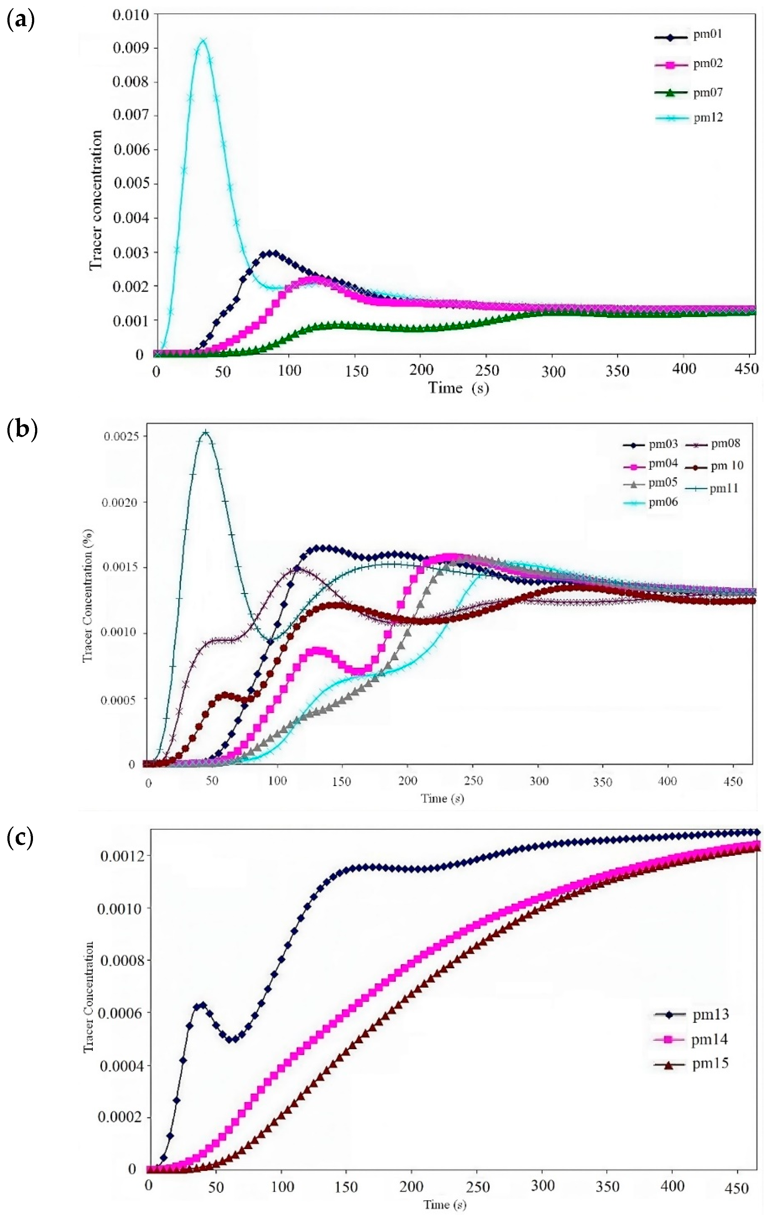
Figure 11a–c show the tracer concentration curves for different zones. The curves for the monitoring points near the impeller shaft are displayed in
Figure 11a. The strongest influence of the impeller is on the monitoring point (Pm
12). This point is placed very near the injection point; then, it is quickly saturated in excess, showing the highest concentration values. As a consequence, these regions are quickly saturated; thus, only this curve will always remain over the final tracer concentration. Hence, this zone can be considered as a stagnant but also oversaturated region. In other words, a high tracer concentration remains around this zone without being distributed. After this, the tracer concentration is lightly reduced due to a slow distribution. The tracer concentration behavior is a sinusoidal damped curve, and the alternation is evidence of the strong influence provided by the impeller near the injection and monitoring points. This influence is reduced significantly on the point (Pm
7) with an intermediate position on the cylindrical tank. This curve remains without tracers and always is under the final tracer concentration until the homogeneity is reached. But, in the points far away from the impeller such as the monitoring points (Pm
1) and (Pm
2), this influence is very weak. The tracer concentration remains equal to zero, during the initial 25 s; the tracer is slowly dispersed and delays on arriving toward these zones. This behavior can be attributed to the joining between the shaft and the flat liquid surface. Finally, all the curves in
Figure 11a are sinusoidal, and the homogenization is reached after 350 s, indicating a good mixing.
The monitoring points near the tank walls are shown in
Figure 11b. The monitoring point Pm
11 shows a similar behavior than the point Pm
12. The tracer concentration is quickly increased. Although the tracer concentration value is considerably more minor than in point (Pm
12), the sinusoidal behavior is also similar. Nevertheless, this point reaches the final tracer concentration value faster than the point Pm
12 due to its fluctuations being lower. The points in the middle of tank body such as the Pm
8, Pm
9 and Pm
10 also show a sinusoidal behavior, but these points remain briefly with a tracer concentration equal to zero; then, they begin to increase its tracer concentration. These curves always remain below the final tracer concentration value until reached. Curves for the points in the faraway positions such as Pm
3, Pm
4 and Pm
5 also remain below the final tracer concentration during the first 120 s and are damped curves due to the slow mixing process. Finally, the tracer concentration in the lowest region of the semispherical reactor has longer times without change (C
tracer = 0), as is shown in
Figure 11c. The curves for the monitoring points Pm
14 and Pm
15 are parabolic due to the tracer being slowly dispersed here. Nevertheless, the curve for the point Pm
13 is sinusoidal due to this point being the nearest to the impeller. These three curves also remain always below the final tracer concentration value: evidence again that the bottom is the most complicated region for distribution.
8. Validation of Hydrodynamics
Instability in tracer distribution curves is at the beginning of the time simulation due to the tracer being placed at a specific point and beginning to be distributed as the fluid forces impulses to move. Instability (tracer concentration variation) is the criterion to minimize the time required to obtain a homogeneous tracer distribution all around the tank. All simulations for every different injection point tend to be a common value. Then, the goal is to obtain the final tracer concentration in the shortest time.
Numerical methods and computer simulations have become a powerful tool to solve old complex problems. Increasing data store and management makes it possible to obtain accurate results quickly. Then, in this research, discretization of the lead volume on the tank was completed using different meshes. Information about these meshes used for discretization of the tank, impeller and lead volume is in
Table 3. The tank and impeller are 3D bodies which were discretized using 2D meshes over their surfaces and then incorporated to the simulation. The lead volume inside was subtracted from the tank, and the impeller was defined and meshed using triangular, squared and hexagonal 2D elements which form tetragonal, hexagonal and honeycomb 3D meshes. The lead volume represented by every 3D cell is a tetragonal cell 9.676 × 10
−7 m
3, hexahedral cell 9.6594 × 10
−7 m
3, and honeycomb cell 9.71766 × 10
−7 m
3, respectively; these are similar volumes which were selected to measure the efficacy of meshes.
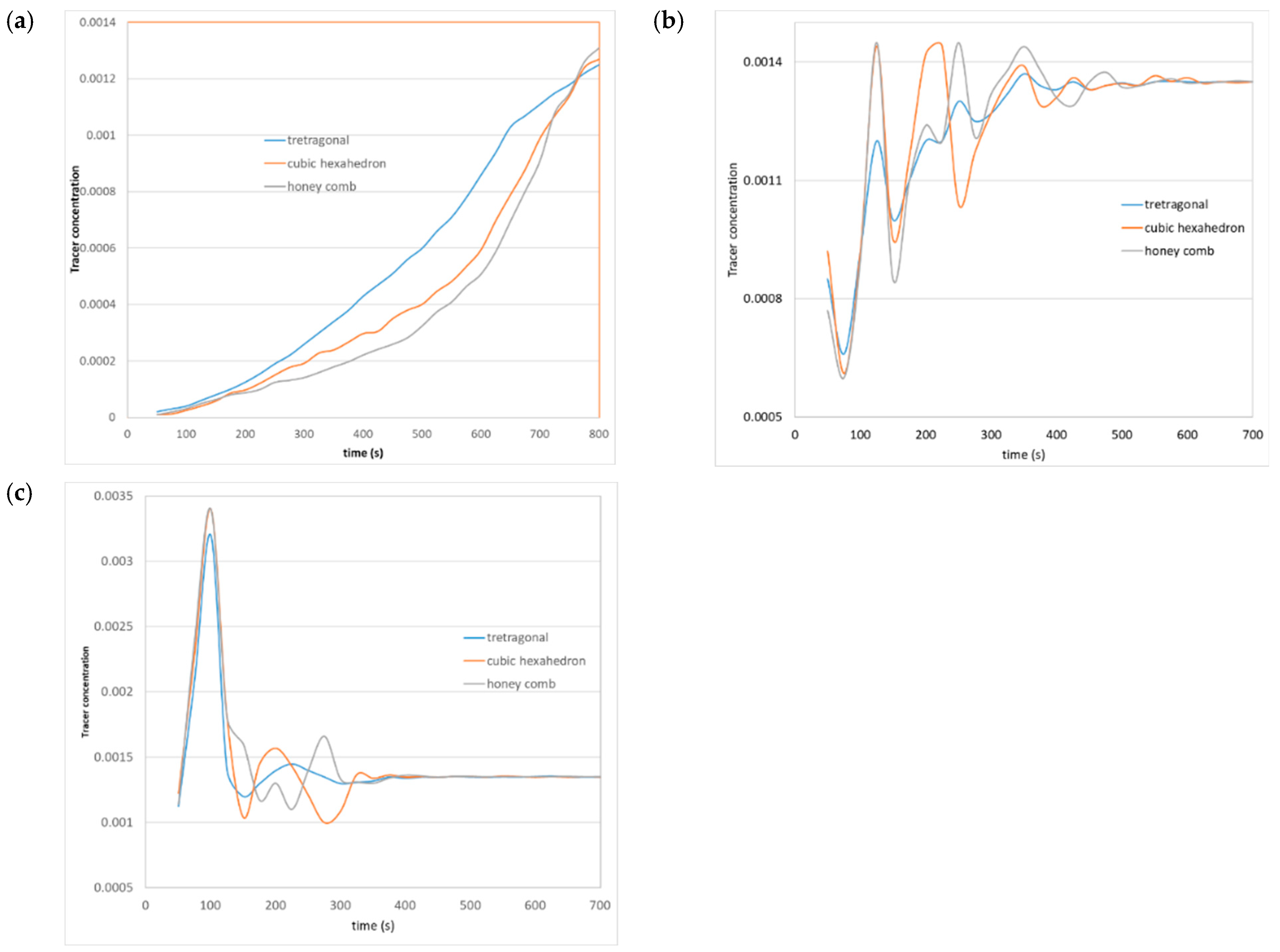
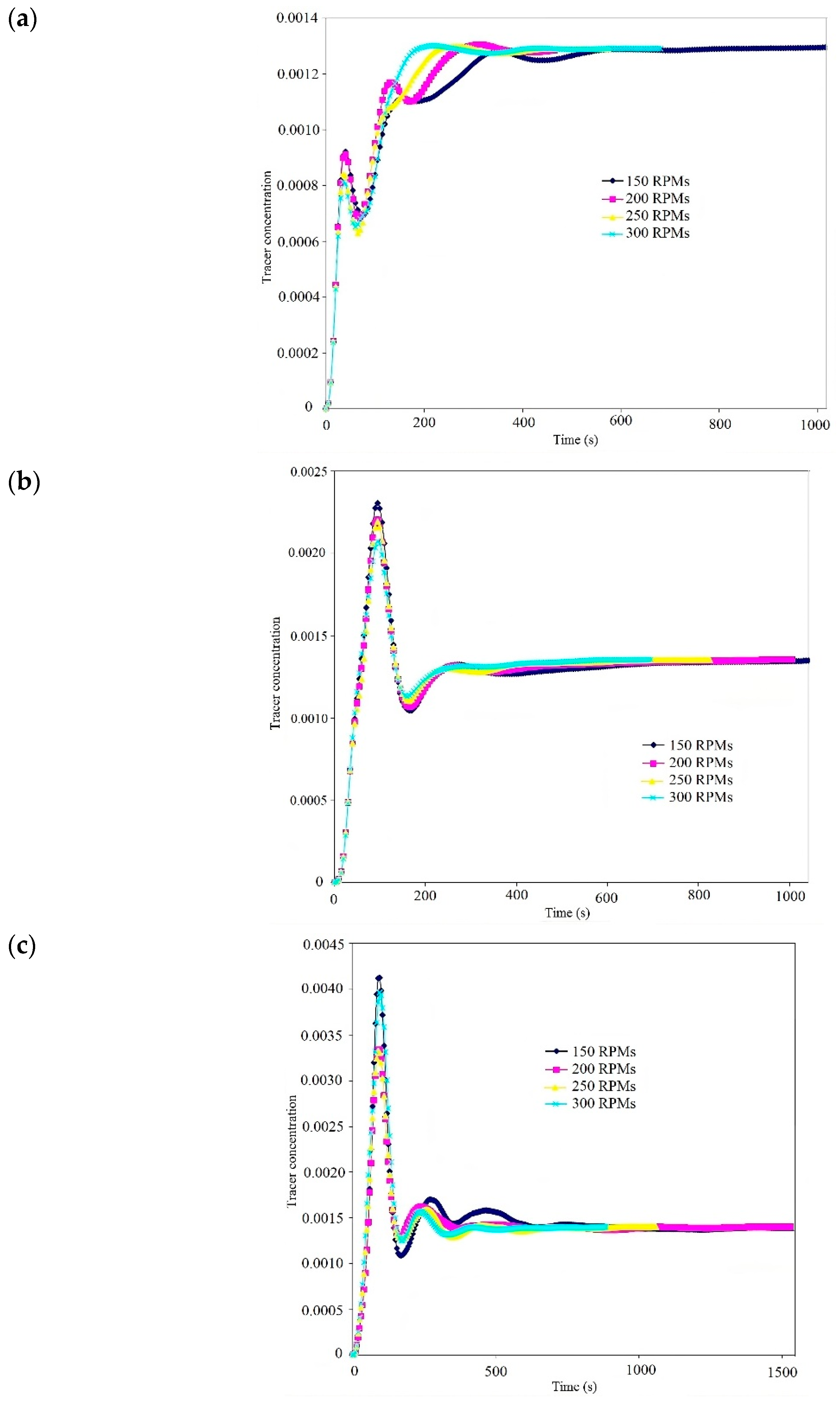
A comparison of results using hexahedron and honeycomb meshes is shown in
Figure 12,
Figure 13,
Figure 14,
Figure 15 and
Figure 16, taking the previously mentioned injection points (P
i=21, P
i=18, and P
i=11). Here, all the solutions tend to the final tracer concentration; then, it is possible to affirm the model works and results are reliable. Nevertheless, at the beginning of the simulation, there are notorious differences regarding approaching and variations. Simulations for the injection point P
i=21 is with a parabolic form due to the final tracer being slowly distributed from points near the top. Consequently, it takes longer for the tracer delay to be distributed. In contrast, simulations for the points P
i=18 and P
i=11 are with a sinusoidal form due to there being a dynamic tracer interchange as a result of the impeller movement, but the tracer is quickly distributed. Then, it is also possible to say all meshes tend to final tracer concentration, but the tetragonal mesh has reduced fluctuations. Additionally, the transitory states are the most complicated to calculate.
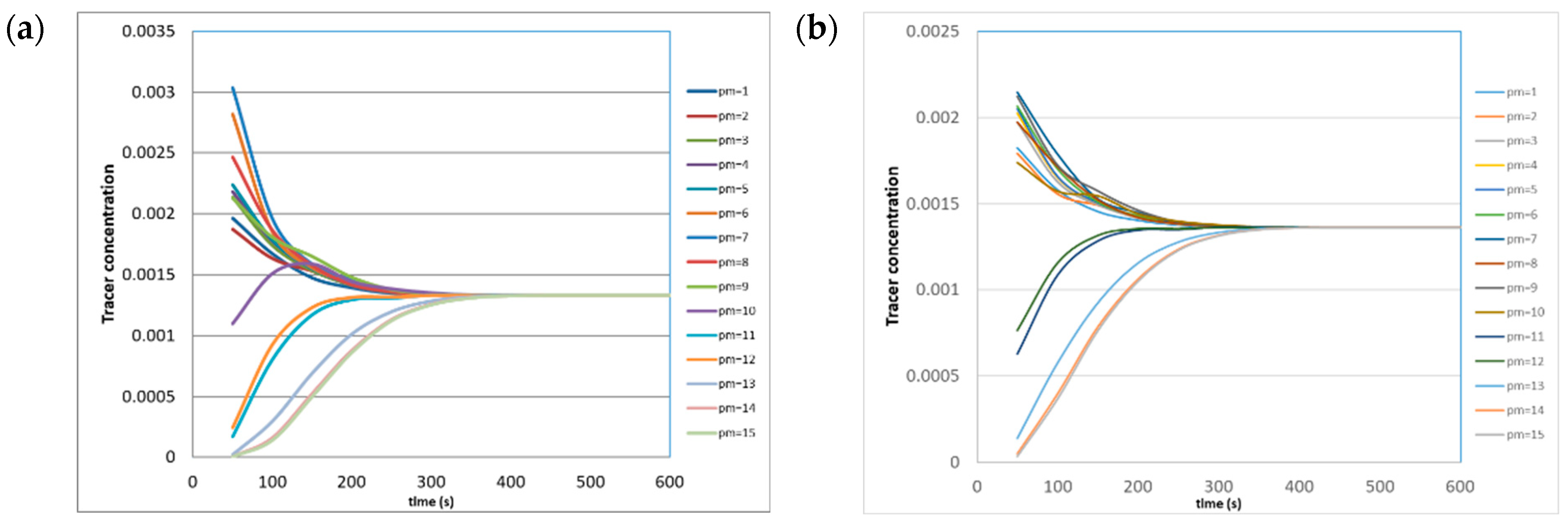
Additionally, for comparison, the tracer concentration resulted for the injection points P
i=1, and P
i=9 on every monitoring point is shown in
Figure 13a,b. Here, again, all curves tend to the final tracer concentration value, evidencing that this value can be considered as a feasible criterion for a homogeneous distribution. Some points near the impeller tend to the final tracer concentration, but other delays are longer. Then, the difference on tracer concentration is a measure of the hydrodynamic difficulty to distribute the tracer on every tank zone. Here, again, it is possible to appreciate that the tracer concentration variations are minor on all monitoring points for the injection point P
i=9. It is possible to appreciate that monitoring points near the impeller tends to the final tracer concentration quickly, and that monitoring points placed near the injection points are with a notorious tracer excess. In contrast, monitoring points on the semispherical zone have a tracer deficit.
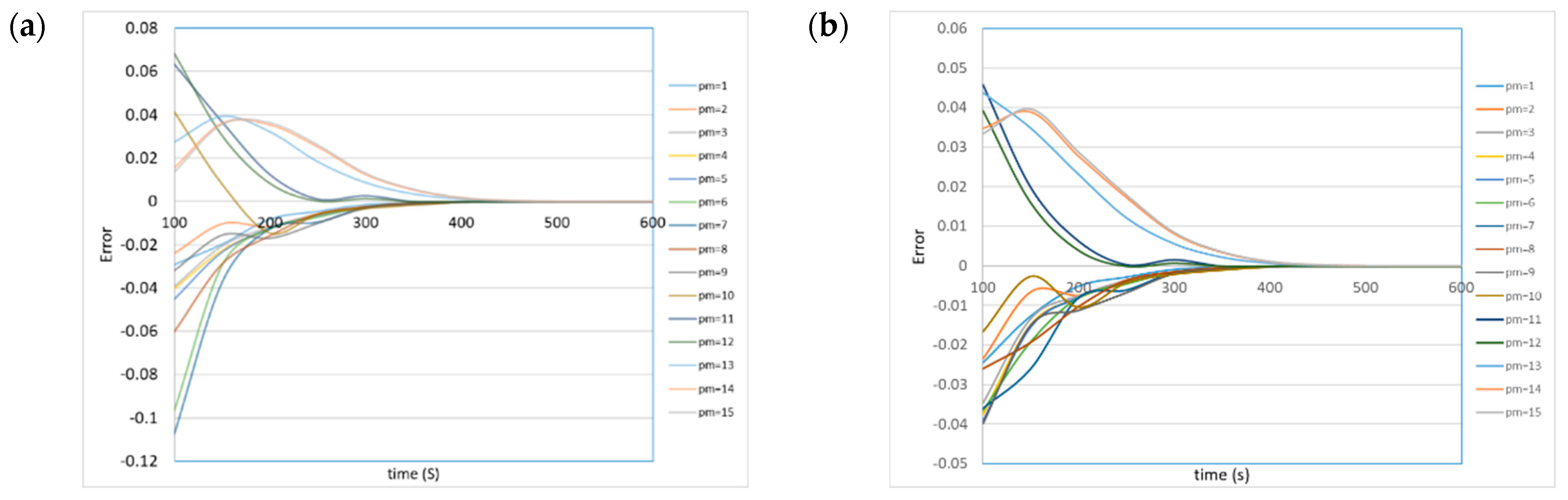
To know the homogeneity of the tracer distribution, Equation (13) was used to calculate variations respecting the last calculated values; then, the curves for every monitoring point tend to zero when the tracer has been homogeneously distributed, as shown in
Figure 14a,b.
Injection points P
i=21, P
i=1, P
i=2 and P
i=6 are with similar behaviors and are the most complicated for distribution; these points are near the upper wall and top of the tank. The tracer placed in these points initially is very far from the impeller influence. Velocity vectors are weak, and the inertial forces of the fluid move the tracer so slowly. An additional handicap against tracer distribution is the fact that properties of the tracer and melting lead are the same (ρ
tracer = ρ
lead); consequently, the influence of the buoyancy forces makes difficult to drive the tracer to the bottom of the tank. Industrially, this can be a serious problem if the density of the reacts added for the cleaning lead is equal to or less than lead density (ρ
tracer < ρ
lead). Then, the industrial suggestion was to place the reacts near the bottom tank. Moreover, the vector in the semispherical bottom impulses up the fluid. In the same way, the injection points P
i=18, P
i=19, P
i=20 and P
i=22 form a common area; these are the best injection areas due to the influence of the impeller being near. Then, the place tracer can be strongly impulsive, while tracer concentration on the semispherical zone and near the impeller influence denotes a very different hydrodynamic behavior, as can be seen in
Figure 15a,b.
Finally, a comparison with a physical model is shown in
Figure 16a–c. Here, it is evident for short times, there is a notorious difference between the computational mode using tetrahedral mesh and a model that was built. The physical model was built with a transparent acrylic: the scale was 1:11, the fluid used for representing lead was water, and the tracer was sodium chloride. A particle indicator velocimeter was used to measure the quantity of tracers passing across every monitoring point position. In these figures, there is also a tendency to the final tracer concentration calculated computationally, although variations can be appreciated during the transitory period due to the natural turbulence of the physical modeling.
Consequently, after the hydrodynamic analysis, the following criterion for identifying an improvement on the mixing process can be confirmed.
Curves of tracer concentrations tend to approach the final tracer concentration faster; thus, mixing time is reduced.
Fluctuation of the tracer concentration curve is minor.
Tracer in excess is minor, and it is quickly distributed.
Instability at the beginning of simulation is high, and the major variations between the physical model and computer simulations are at this instant of the simulation.
Inject reacts for cleaning in different points of the tank is the easiest way for modifying the industrial practices; then, this work represents the most economic form for improving. Suggestions for future works are to simulate the system including different properties for the tracer (ρtracer ≠ ρlead) and modify the tracer volume at the initial condition to know if there is enough for the cleaning process or if the tracer volume can contribute to reduce the mixing time. Another option to explore is to simulate different tank configurations and different impeller configurations.
In addition, a comparison of simulations using different fine tetragonal meshes is shown in
Table 4. Here, values of the stirring times required to obtain the final tracer concentration using the injection points P
i=21, P
i=18 and P
i=11 are employed to test the mesh influence. Fine mesh is expressed as a percentage of nodes listed in
Table 4. Thus, a 200% mesh has double the nodes for discretization. Here, it is evident that the times vary with wider meshes, but its influence is reduced as the mesh became smaller.
10. Conclusions
After analyzing of the cases simulated, the following conclusions can be drawn.
The tracer concentration in the monitoring points near the impeller is strongly influenced by the rotational speed and strong fluctuations of the tracer concentration can be observed; nevertheless, the tracer excess quickly is distributed due to the stirring.
Sinusoidal curves for tracer concentration are evidence of the instability of the system; the tracer here must be distributed to improve mixing; until all these curves are damped, the tracer concentration will tend to be homogeneous.
There are curves with sinusoidal and parabolic behavior; parabolic curves were frequently found in the bottom of the tank or near the surface of the tank due to these points being far away from the impeller influence. Consequently, parabolic curves always have a deficit of tracer concentration, and its presence indicates a poor mixing zone.
According to the simulations, it is unnecessary to run longer times due to the tracer having been homogeneously distributed, and the variation of concentration values is not significant. Consequently, employing extra times for mixing is also unnecessary.
The evolution of tracer concentration is a feasible parameter to evaluate mixing; it is evidence of a homogeneous distribution. Moreover, understanding the hydrodynamic dynamics inside the stirred lead reactor is very important to improve its performance.
The selection of the best injection point is very important to reduce unnecessary working times and improve industrial efficiency.
According to the simulations, it is possible to affirm that the tracer must be injected near the impeller in order to profit from the stirring forces. Therefore, the injection of a tracer on points near the top surface or reactor walls must be avoided due to these having the most delayed mixing times.
The semispherical region at the tank bottom is the most complicated region in which to distribute the tracer due to buoyancy forces, which force up the liquid. This reactor can be redesigned; a flat bottom configuration improves mixing.


