Abstract
This paper focuses on the geometrically nonlinear dynamic analyses of a three-layered curved sandwich beam with isotropic face layers and a time-dependent viscoelastic core. The boundary conditions and equations of motion governing the forced vibration are derived by using Hamilton’s principle. The first-order shear deformation theory is used to obtain kinematic relations. The spatial discretization of the equations is achieved using the generalized differential quadrature method (GDQM), and the Newmark-Beta algorithm is used to solve the time variation of the equations. The Newton–Raphson method is used to transform nonlinear equations into linear equations. The validation of the proposed model and the GDQM solution’s reliability are provided via comparison with the results that already exist in the literature and finite element method (FEM) analyses using ANSYS. Then, a series of parametric studies are carried out for a curved sandwich beam with aluminum face layers and a time-dependent viscoelastic core. The resonance and cancellation phenomena for the nonlinear moving-load problem of curved sandwich beams with a time-dependent viscoelastic core are performed using the GDQM for the first time, to the best of the authors’ knowledge.
1. Introduction
The beams, which are made of conventional isotropic materials, have been studied by many researchers for decades. However, in recent years, with the rapid development of manufacturing and material technologies, studies about new kinds of materials, namely composites and FGM, have been attractive so far. Nonetheless, sandwich structures have been widely preferred in the marine, aerospace, civil, and railroad vehicle industries due to their high strength, low weight, and good vibration damping properties. There are many studies devoted to the static, dynamic, and vibration analyses of structures with different kinds of geometries, namely flat, curved, and variable-thickness beams. Also, both linear and nonlinear analyses have been performed so far. Apart from the exact analytical solutions, many numerical methods for solving partial differential equations are found by scientists.
Beams are used in a wide variety of engineering applications, as they are basic structural elements. They are used in rotor blades, shafts, frames, and robotic structures. Flat beam problems are widely found in literature. Singh et al. [1] presented various formulations about the large-amplitude free vibration of beam structures. Gafsi et al. [2] studied the vibration of nonlinear flexible beams with variable geometric properties. After the GDQM was developed by Richard Bellman and his associates in the early 1970s, many studies have been conducted so far. Bert and Malik [3] investigated freely vibrating cantilever beams by using the GDQM. They presented the effect of different sampling points on the natural frequency values by comparing them with the analytical results. Jang et al. [4] studied the application of the GDQM to the static analyses of structural components, such as beams and rectangular and circular plates. Feng and Bert [5] applied the quadrature method for solving flexural vibration problems, including geometrical nonlinearities. They used only one degree of freedom. Karami and Malekzadeh [6] presented a new differential quadrature methodology for stability, static, and dynamic analyses of beams and also calculated the error regarding the number of sampling points. Zhong and Guo [7] performed nonlinear vibration analyses of thick beams with Timoshenko beam theory using the GDQM and mostly computed the ratio of the linear frequency to the nonlinear frequency. Ghasemi and Mohandes [8] investigated the finite strain effect for nonlinear free vibration analyses of unidirectional composite beams with Timoshenko beam theory by using the GDQM. Mahmoud et al. [9] used GDQM for free vibration analysis of delaminated beam plates. Eftekhari conducted several studies of beams and plates on both linear [10,11,12] and nonlinear [13] dynamic problems, specifically for moving loads using the GDQM. He investigated many effects, such as sampling points and Dirac-delta function coefficients. He found perfect agreement with the analytical solutions.
Also, several studies are found in the literature for curved beams. Yang and Yau [14] investigated the dynamic response of horizontally deep-curved beams under both horizontally and vertically moving loads. Hajianmaleki and Qatu [15] conducted static and vibration analyses for thick and generally laminated deep-curved beams with various boundary conditions. Poojary and Roy [16] used the finite element method in order to study the in-plane vibration of curved beams under moving loads. Moreover, the GDQM is also used to solve problems with curved beams. Kurtaran [17,18] used the GDQM for solving several large displacement transient and static analyses of curved beams. Nikkhoo et al. [19] applied the GDQM in order to study the dynamics of curved beams under moving loads. Kang et al. [20] performed vibration analyses for horizontally curved beams with warping using the GDQM. It is also possible to use the GDQM for solving more complex structural problems than beams, such as plates and shells. Akgün and Kurtaran [21] performed transient analyses of laminated composite super-elliptic shells with geometrical nonlinearities using the GDQM. Malik and Bert [22] showed the implementation of multiple boundary conditions for the GDQM solutions of higher-order partial derivative equations, which govern the free vibration of the plates. Fung [23] solved dynamic problems using the GDQM and examined the stability and accuracy of the method. Most of the sampling point types are used, such as Legendre, Radau, Chebsevey, Chebyshev–Gauss–Lobatto, and uniformly. Bacciocchi et al. [24] also conducted a vibration analysis of variable-thickness shells and plates using the GDQM.
Viscoelastic materials are widely preferred in sandwich structures due to their vibration and energy damping properties. Azevedo and Coben [25] performed a dynamic analysis of a viscoelastic Timoshenko beam numerically using the Kelvin–Voigt material model. Chen and Lin [26] conducted a dynamic analysis of viscoelastic material by incremental FEM. Shafei [27] investigated the nonlinear transient vibration of viscoelastic plates with a NURBS-based iso-geometric higher-order shear deformation theory approach. Tolpekina et al. [28] studied both linear and nonlinear viscoelastic moduli of rubber materials by creep compliance and stress relaxation analyses. Arikoglu [29] made a new fractional derivative linearly viscoelastic material model and parameter identification by genetic algorithms. Demir et al. [30] performed a vibration analysis of a curved composite sandwich beam with a viscoelastic material core layer using the GDQM. Arikoglu and Ozkol [31] and Taskin et al. [32] performed damping and vibration analyses of composite sandwich plates and sandwich cylindrical shells, respectively, in which the core layer is a frequency-dependent viscoelastic material made using the GDQM.
This study aims to predict the nonlinear dynamic characteristics of a three-layered curved sandwich beam with isotropic face layers and a time-dependent viscoelastic core. The boundary conditions and equations of motion governing the forced vibration are derived by using Hamilton’s principle. The first-order shear deformation theory is used to obtain kinematic relations. The spatial discretization of the equations is achieved by using the generalized differential quadrature method (GDQM), and the Newmark-Beta algorithm is used to solve the time variation of the equations. Validation of the proposed model and the GDQ solution’s reliability are provided by comparison with the results in the literature and finite element method (FEM) analyses performed via ANSYS. Then, a series of parametric studies are carried out for a curved sandwich beam with aluminum face layers and a time-dependent viscoelastic core. The dynamic analyses of curved sandwich beams with a time-dependent viscoelastic core are performed using GDQM. Cancellation and resonance phenomena have been studied widely for linear moving load problems; however, it is the first time these phenomena have been considered for a nonlinear problem to the best of the authors’ knowledge.
2. Theory and Formulations
2.1. Kinematics, Constitutive, and Equilibrium Equations
The governing equations are derived from Hamilton’s principle. To obtain the equation of motion of a curved beam, some assumptions are made as follows:
- The connection between layers is simply perfect, so delamination does not occur.
- First-order shear deformation theory is used.
- Face layers are assumed to be incompressible, unlike the core layer.
- Since the deformations are not small, Von Karman-type nonlinear strain terms are included.
Displacement relations of the layers are obtained for the sandwich beams, which require continuity and are represented in Figure 1 between the face layers for , where subscript represents the layer number.
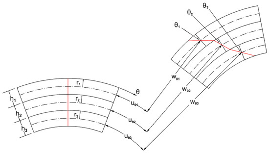
Figure 1.
Coordinate system, configuration, and representation of beam layers.
For the viscoelastic core layer:
Regarding the beam theory with Von Karman-type nonlinearity, the above displacement relations are obtained. Here and represent the circumferential and radial displacements of the beam, respectively. , , and represent the circumferential displacement, radial displacement, and circumferential rotation of mid-surface of the beam, respectively. and are the radial rotation of the core layer and the circumferential coordinate. The displacement relations of the core layer can be expressed in terms of the face layers to eliminate 1/3 of the degrees of freedom as follows:
Kinematic relations of the ith layer of the beam structure for cylindrical coordinates can be expressed by the Von Karman nonlinear theory for large displacements for , where superscript represents the layer number.
By using the generalized Hooke Law, the stress-strain relation of the isotropic materials can be written for beams as follows for :
Although shear strain is the most dominant for viscoelastic materials, strains in radial and circumferential directions are not neglected. The Lagrangian equation is energy conservation, which is the sum of kinetic energy K, potential energy P, internal strain energy U, and external force work V in this case. By using Hamilton’s principle, the equation of motion can be obtained, as shown below:
By inserting the constitutive relations (5) into Equation (6), the first variation of the energy terms can be obtained for :
Here and represent width of the beam, density, distributed load, radius of curvature, and time derivative for the ith layer. Thus, governing equations and natural boundary conditions can be derived by inserting the kinematic relations (4) into Equation (7). From constitutive relations together with energy equations, the Euler equations are obtained for the dynamic analysis of sandwich beams in terms of cross-section forces and moments for and , respectively, as presented in Appendix A.
2.2. Generalized Differential Quadrature Method
The Differential Quadrature Method is a numerical method for solving partially differential equations that was founded in 1971 by Bellman and his associates. It basically converges the partial derivatives of a discrete point with respect to spatial derivatives to the functional values of the same discrete point, which is in the domain. The main motive to develop this method is that the necessity of the grid points to solve the problem is far less compared to other numerical methods, such as the central difference method. When GDQM is first developed, the results are partially bad for solving greater systems, but then Shu and his associates developed another method, the generalized differential quadrature method, to overcome this problem.
The derivation of a function at a discrete point with respect to a spatial variable is predicted by the weighted linear summation of the functional values of all discrete points in the domain as follows:
Here M represents grid numbers in the direction and represents weighted coefficients. The first-degree partial derivative is obtained as weighted coefficients as follows:
The derivation of with respect to is described as follows:
To obtain weighted coefficients for higher-degree partial derivatives, the below formulation is used as follows:
In the method, grid numbers and distribution have a significant effect on the solution. When the grids are determined to be equally spaced, Runge’s phenomena occur. To overcome this issue, the Chebyshev–Gauss–Lobatto grid distribution is applied as follows:
2.3. Time Integration, Linearization of the Equation of Motion, and Viscoelasticity
2.3.1. Newmark-Beta Method and Newton–Raphson Method with GDQM
The Newmark-Beta Method is an integration scheme that is used for solving time-dependent differential equations implicitly. It is based on the two equations below.
Here, and describe the variation of the acceleration with respect to the time step and determine the accuracy and stability of the method. While and , it is named the average acceleration method, stability is not affected by the size of the time step. In the solution of the initial value problem, the equation of motion for the ’st time step can be written as follows:
Rearranging the equation above, acceleration and velocity at the ’st time step can be described as follows:
Thus,
where
Here, and represent the effective stiffness matrix and effective load vector, respectively.
Unlike linear systems, the stiffness matrix depends on the displacement value, which can be described as . While is calculated iteratively, the matrix needs to be linearized. The Newton–Raphson method is widely used for these systems. For more detailed algebra, chapter 5 of the book “Dynamic of Structures” by Chopra [33] can be seen.
For this problem, the curved beam domain is discrete to points. While sacrificing the boundary grids for the boundary condition equations, the inner grids for the governing equations would be for one degree of freedom. Thus, three degrees of freedom are used for this problem, namely. Thus, the beam domain would have points in total, and the solution domain would have points. The governing equation for the dynamic analysis can be written in matrix form as follows:
where is the linear stiffness matrix and is the nonlinear stiffness matrix with the dimensions of . and are displacement and load vectors with the dimensions
The nonlinear Equation (33) is solved by the Newton–Raphson method. The nonlinear matrix can be derived from the displacement vector and the tangential stiffness matrix is obtained as follows:
Applying the Newton–Raphson method to the governing equation results in the following:
where the residual matrix is as follows:
Iterations continue until the error is minimized to a certain value, i.e., at The iteration is described as follows:
For more detailed algebra, chapter 9 of the book titled “Differential Quadrature and Differential Quadrature Based Element Methods: Theory and Applications” by Wang [34] can be seen.
2.3.2. Viscoelasticity
For the generalized Maxwell model, stress can be written in the following form:
where and are creep compliance coefficients and and are elastic and inelastic strain terms of the generalized Maxwell model. The stress tensor of the material is described in terms of the creep compliance function, which means the specimen would have a stress value at time t when a constant strain is applied as a Heaviside step function at time t.
where are the creep compliance coefficients of the generalized Maxwell model and is the viscous damping constant. Using these equations, the first-order differential equation is obtained as follows:
where , and by using the Laplace transformation, the first-order differential equation is solved for inelastic strain, and it gives the following:
Substituting this solution into Equation (A5), stress can be described in terms of elastic and inelastic strain as follows:
where s represents the integrant time variable for the Laplace transformation rule.
To model the viscoelastic material in this problem, the multiaxial case of the time-dependent generalized Maxwell model is used. As a convolution equation over time that requires a high computational cost, the below equation is rewritten in incremental form, in which time integration is used numerically.
where and represent the viscous damping constant and constitutive matrix, respectively. Dividing the integral into two parts, in which the first part is from - to t and the second part is from t to . Then, by applying the trapezoidal rule to the second part and rearranging the equation, the stress term can be obtained as follows:
The first and second terms of the right-hand side of Equation (33) represent internal forces for the viscoelastic layer at the previous time step, which are and are calculated by using the kinematic and constitutive relations (4-5) by using calculated displacement values as shown in Equation (14) at the previous time step. Then, these vectors are extracted from the external force vector in Equation (22) as shown in Equation (A3) in Appendix A and are represented as and . The third term of the right-hand side of Equation (33) represents the multiplication of stress terms and the first variation of strain terms at the initial time step is for the viscoelastic layer in energy (Equation (7)). For more detailed algebra, chapter 6 of “Nonlinear Dynamics of Structures” by Oller can be seen [35].
3. Validation Studies
In this section, three different problems are investigated to determine the accuracy and validity of modeling geometric nonlinearities, moving loads, and viscoelasticity, as follows:
3.1. Example 1
The problem setup with simple supported boundary conditions and moving loads can be seen in Figure 2.
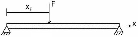
Figure 2.
Moving point load on the simply supported beam.
In this section, analyses are made to determine the accuracy and validity of the present method. The results are compared with the literature in which the forced vibration of a beam due to a moving load is solved by Eftekhari [10]. In the problem, a concentrated F load moves from one end to the other with a constant velocity for each case in t time, and the response of the beam center is investigated. In order to model point load as a distributed load, an exponential function behaving similar to the Dirac-delta function is introduced:
where F, v, t and represent the amplitude of the point load, velocity of the point load, time, and regularization parameter, respectively, for the beam with n grid points. For a more detailed expression of the function, an article by Eftekhari [10] can be seen.
In the graphs below, and represent the dynamic response of the beam center and static displacement of the beam center, respectively. Dividing with results in the normalization of the results. Also, the time required for the point load to travel through the beam is divided by the period for normalization as well. The results are compared to the exact solution values in the article. Data digitization is used to determine values. The geometric and mechanical properties of the sandwich beam are considered in the problem under a moving load with an amplitude of 4.45 N, as given in Table 1 below:

Table 1.
Description of the moving load problem.
In Figure 3, a convergence study is also made for 31, 41, and 51 grid points. However, instabilities are observed for 21 grid points, which are not shown in the graphs. Different from the validation article, the Dirac-delta coefficient and time interval values are 0.005 and 200, respectively. It can be seen that convergence of the grid points occurred earlier for higher velocity values.
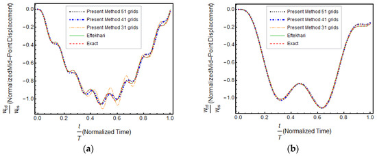
Figure 3.
Comparison of the results for two different velocity values: (a) 15.6 m/s and (b) 46.8 m/s.
3.2. Example 2
Now we consider Example 1 by adding geometrical nonlinearities. The results are compared with the explicit FEM analyses performed by ANSYS. In GDQM analysis, 51 grid points are used, and a forced vibration response is obtained. Equivalent mass damping with is used to simulate viscoelastic behavior. However, normalization of time and displacement is not made in this case. The time history of the beam center is observed again. As can be seen in Figure 4, a good agreement is observed.
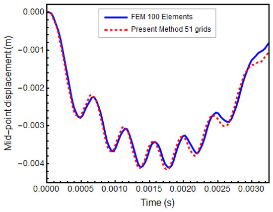
Figure 4.
Comparison of the results for 31.2 m/s.
3.3. Example 3
In this example, the nonlinear transient response of a semi-circular viscoelastic arch subjected to pressure load in the reverse normal direction, as shown in Figure 5, is analyzed. Again, 51 grid points are used to investigate the mid-point displacement of the arch. A load is applied to the model with the Heaviside step function. In addition, load is applied in two steps as half amplitude for each 12,501-time interval. The circular-arch modeling parameters are presented in Table 2.
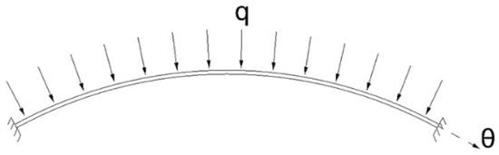
Figure 5.
Distributed load on the fixed circular arch.
Table 2.
Problem data for the circular arc.
The finite element model is built by solid elements, and the external load is applied as a pressure load. The model consists of 600 solid elements, 1212 nodes, and 7272 degrees of freedom, and it is constrained so that only in-plane motion is allowed. On the other hand, the pressure load is multiplied by the beam’s width and converted to a distributed load acting on the circular arch in a reverse normal direction.
Here, ST and LT represent short-term and long-term, respectively. Transverse deflection of the central point and damping are observed under the load. An acceptable agreement is observed from the results, as shown in Figure 6.
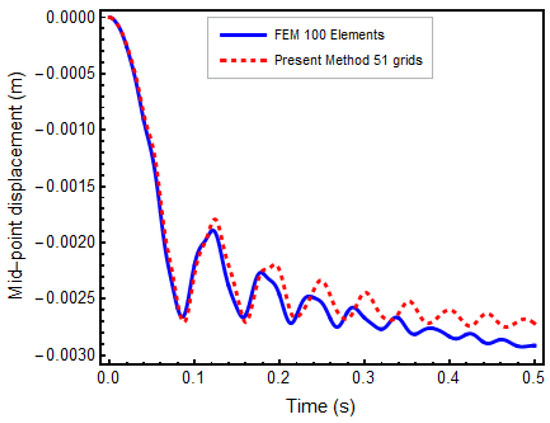
Figure 6.
Time history of mid-point displacements.
4. Case Studies
In this section, nonlinear dynamic analyses of a three-layered curved sandwich beam are presented. Aluminum material is used for the face layers, while viscoelastic material is used for the core layer. Fixed boundary conditions are applied on both ends. The moving point load is applied in two load steps on the top layer towards the arc center, as shown in Figure 7, and the response of the beam center on the top layer is calculated.
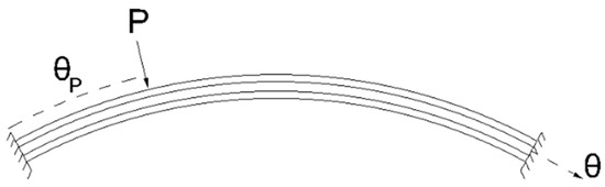
Figure 7.
Curved sandwich beam representation under moving load.
4.1. Sandwich Beam Subjected to Moving Load (Forced Vibration)
For this case, the thicknesses of the top, core, and bottom layers are fixed at 0.3 mm, 0.4 mm, and 0.3 mm, respectively, which results in a total 1 mm arch thickness. For all parametric analyses, the Dirac-delta coefficient is 0.005. The constant average acceleration method is used in the Newmark-Beta formulation. Viscoelastic material, which is introduced in Example 3. The geometry and material properties of the problem and the parameters of the solution procedure are listed in Table 3 below:
Table 3.
Problem data for the present method.
In total, 2146 parametric analyses are conducted in order to investigate the effect of the curvature of the beam under certain load amplitudes and velocity values. Maximum displacement and oscillation in the transverse direction of the beam center are mainly investigated. The length of the beam arc is held constant, while the radius of curvature and arc angle are parametrically varied. The results have converged for 55 grid points for the problem considered. The amplitude of the loads is chosen to satisfy the requirement that the maximum displacement-total thickness ratio of 1 is exceeded to observe the nonlinear effects.
Increasing displacement is expected with increasing radius of curvature, i.e., the straighter the beam, the larger the displacement in linear analyses. However, this is not observed for all cases considered, as seen in Figure 8, due to the nonlinear effects. Moreover, with decreasing curvature and increasing load amplitude, the frequency of oscillations increases in all cases. Beams recover to the undeformed position when the load exits the beams, only in some cases. It is predicted that the load travel frequency does not match the natural frequency of the beam.
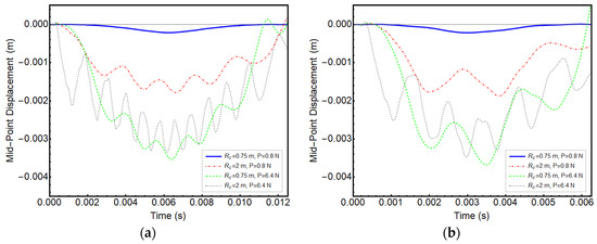
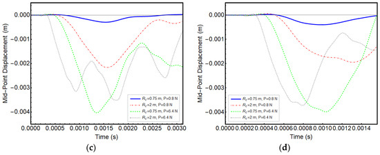
Figure 8.
Time history of mid-point displacements: (a) 8 m/s, (b) 16 m/s, (c) 32 m/s, and (d) 64 m/s.
From Figure 9a,b, it can be clearly seen that the displacement of the beam center first increases with the increasing value of the load velocity, then decreases. On the other hand, displacements increase with the load amplitude, as expected. It can be said that there is a nonlinear relationship between the displacement, velocity, and load amplitude.
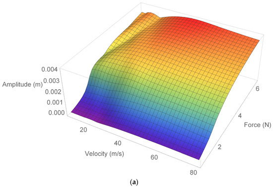
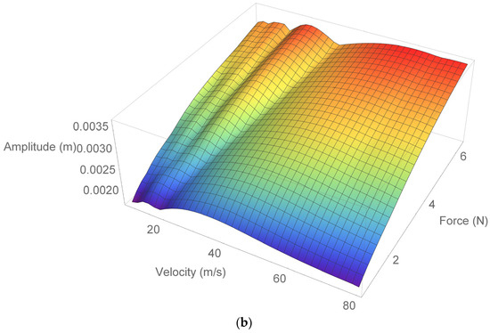
Figure 9.
Present method results: (a) and (b) .
4.2. Sandwich Beam Subjected to Moving Load (Free Vibration)
In this section, the free oscillation of the beam is investigated after the load is removed. Different from Section 4.1, the thicknesses of the top, core, and bottom layers are fixed at 1 mm, which results in a total of 3 mm of arch thickness. The radius of curvature is 1 m, and the long-term shear modulus of the viscoelastic material is 3.5 mPa. In total, 30,576 parametric analyses were done to observe cancellation and resonance phenomena for cantilever beams. In the literature, simply supported beams are widely studied for this phenomenon [14].
Figure 10 shows the variation of maximum mid-point displacement with load amplitude and velocity after the load leaves the beam. It is observed that for loads with relatively lower amplitude, both the cancellation and resonance velocity values decrease with the increasing load. In contrast, the resonance and cancellation velocity values increase with increasing load for the loads with relatively higher amplitude. It can be said that the ratio of load effect frequency to structural natural frequency is not the only parameter that determines the cancellation and resonance phenomena but also the amplitude of the load. This result can be supported by the effect of force amplitude on nonlinear frequency response functions due to geometrical nonlinear effects, which can be found in the literature. The displacements for minimum and maximum load cases, i.e., 1 N and 26 N, respectively, are presented in Figure 11 for a closer inspection.
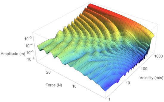
Figure 10.
Variation of maximum amplitude with force and velocity.
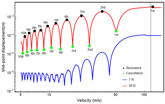
Figure 11.
Variation of maximum amplitude with velocity.
Time histories of the beam mid-point under load with a 26 N amplitude where cancellation and responance are observed are also presented in Figure 12 and Figure 13, respectively. Time history variation with the first, second, third, fourth, fifth, and sixth cancellation velocity values in Figure 11 corresponds to Figure 12a–f, respectively. Furthermore, as seen in Figure 12, there are n number of oscillations during forced vibration in which the time history is symmetrical, which corresponds to the nth value of cancellation velocity. The travel time of the load from one end to the other is one-third of the total analysis time; hence, the free vibration duration is twice as long as the forced vibration duration. However, instead of a complete cancellation, residual responses are observed, as in [14]. Another interesting point is that in the free vibration zone, higher modes are observed with increasing cancellation velocity values, as Figure 12 shows. Time history variation with the first, second, third, fourth, and fifth resonance velocity values in Figure 11 corresponds to Figure 13a–e, respectively. It can be seen that higher modes are not observed for all resonance velocity values.
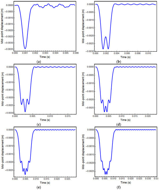
Figure 12.
Time history of mid-point displacement under 26 N: (a) 51 m/s, (b) 26.4 m/s, (c) 17.6 m/s, (d) 13.08 m/s, (e) 10.48 m/s, and (f) 8.72 m/s.
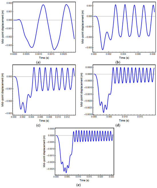
Figure 13.
Time history of mid-point displacement under 26 N: (a) 123.4 m/s, (b) 36.5 m/s, (c) 22 m/s, (d) 15.36 m/s, and (e) 11.76 m/s.
4.3. Sandwich Beam Subjected to Multiple Moving Loads (Forced Vibration)
However, when the beam is excitated by eight moving loads with a 26 N load amplitude and a distance of the beam length between all eight loads, the time history of the mid-point displacement is shown in Figure 14. Resonance phenomena are observed at 118.4 m/s velocity, which does not coincide with the resonance condition for a single moving load. The resonance velocity for the forced vibration response for eight consecutive moving loads is represented by a vertical line in Figure 11 that does not coincide with the resonance velocity of the free vibration response of a single moving load. This is possibly due to the nonlinear effects associated with the large strain analyses of the structure.
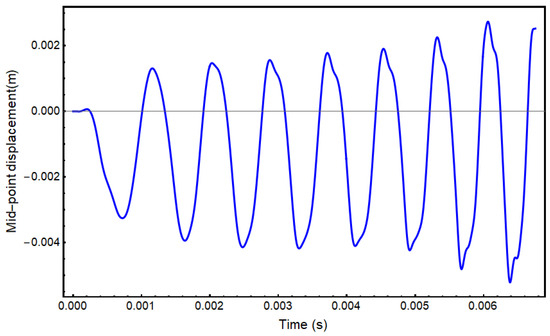
Figure 14.
Time history of mid-point displacement under eight moving loads under 26 N.
5. Conclusions
Vibration analyses due to the moving point load are carried out by both GDQM. Also, validation analyses are conducted by ANSYS and literature, and good agreement is observed even though beam geometry is modeled in polar coordinates and first-order shear deformation theory is used for the kinematic results.
- Increasing the radius of curvature does not cause an increase in mid-point displacement for all cases within the forced vibration.
- Resonance and cancellation velocity values change with the load amplitude due to the nonlinear effects.
- The load travels with the nth cancellation velocity, causing n number of oscillations during the forced vibration, in which the time history of the mid-point is symmetrical.
- The resonance velocity for the beam is not the same for the free vibration condition after leaving a single moving load and the forced vibration condition with multiple moving loads.
For a wider range of parametric analyses, i.e., deeper curved beams, curvilinear coordinates and higher-order shear deformation theory can be used for improvement.
Author Contributions
All authors contributed to the study’s conception and design. Material preparation, data collection, and analysis were performed by M.M.S., O.D. and A.A. The first draft of the manuscript was written by M.M.S., O.D. and A.A., and all authors commented on previous versions of the manuscript. All authors have read and agreed to the published version of the manuscript.
Funding
This research received no external funding.
Data Availability Statement
Data are contained within the article.
Conflicts of Interest
The authors declare no conflicts of interest.
Appendix A
In addition, the natural boundary conditions for and are derived respectively as below:
where m and n represent and for . Forces and moment resultants can be described as:
References
- Singh, G.; Sharma, A.K.; Venkateswara Rao, G. Large-amplitude free vibrations of beams—A discussion on various formulations and assumptions. J. Sound Vib. 1990, 142, 77–85. [Google Scholar] [CrossRef]
- Gafsi, W.; Najar, F.; Choura, S.; El-Borgi, S. Confinement of Vibrations in Variable-Geometry Nonlinear Flexible Beam. Shock Vib. 2014, 2014, 687340. [Google Scholar] [CrossRef]
- Bert, C.W.; Malik, M. Differential Quadrature Method in Computational Mechanics: A Review. Appl. Mech. Rev. 1996, 49, 1–28. [Google Scholar] [CrossRef]
- Jang, S.K.; Bert, C.W.; Striz, A.G. Application of differential quadrature to static analysis of structural components. Int. J. Numer. Meth. Eng. 1989, 28, 561–577. [Google Scholar] [CrossRef]
- Feng, Y.; Bert, C.W. Application of the quadrature method to flexural vibration analysis of a geometrically nonlinear beam. Nonlinear Dyn. 1992, 3, 13–18. [Google Scholar] [CrossRef]
- Karami, G.; Malekzadeh, P. A new differential quadrature methodology for beam analysis and the associated differential quadrature element method. Comput. Methods Appl. Mech. Eng. 2002, 191, 3509–3526. [Google Scholar] [CrossRef]
- Zhong, H.; Guo, Q. Nonlinear Vibration Analysis of Timoshenko Beams Using the Differential Quadrature Method. Nonlinear Dyn. 2003, 32, 223–234. [Google Scholar] [CrossRef]
- Ghasemi, A.R.; Mohandes, M. The effect of finite strain on the nonlinear free vibration of a unidirectional composite Timoshenko beam using GDQM. Adv. Aircr. Spacecr. Sci. 2016, 3, 379–397. [Google Scholar] [CrossRef]
- Mahmoud, A.A.; Esmaeel, R.A.; Nassar, M.M. Application of the generalized differential quadrature method to the free vibrations of delaminated beam plates. Eng. Mech. 2007, 14, 431–441. [Google Scholar]
- Eftekhari, S.A. A Differential Quadrature Procedure with Regularization of the Dirac-delta Function for Numerical Solution of Moving Load Problem. Lat. Am. J. Solids Struct. 2015, 12, 1241–1265. [Google Scholar] [CrossRef]
- Eftekhari, S.A. A simple and accurate mixed Ritz-DQM formulation for free vibration of rectangular plates involving free corners. Ain Shams Eng. J. 2016, 7, 777–790. [Google Scholar] [CrossRef][Green Version]
- Eftekhari, S.A. A simple and systematic approach for implementing boundary conditions in the differential quadrature free and forced vibration analysis of beams and rectangular plates. J. Solid Mech. 2015, 7.4, 7.4,374–399. [Google Scholar]
- Eftekhari, S.A. A differential quadrature procedure for linear and nonlinear steady state vibrations of infinite beams traversed by a moving point load. Meccanica 2016, 51, 2417–2434. [Google Scholar] [CrossRef]
- Yang, Y.-B.; Wu, C.-M.; Yau, J.-D. Dynamic response of a horizontally curved beam subjected to vertical and horizontal moving loads. J. Sound Vib. 2001, 242, 519–537. [Google Scholar] [CrossRef]
- Hajianmaleki, M.; Qatu, M.S. Static and vibration analyses of thick, generally laminated deep curved beams with different boundary conditions. Compos. Part B Eng. 2012, 43, 1767–1775. [Google Scholar] [CrossRef]
- Poojary, J.; Roy, S.K. In-plane vibration of curved beams subjected to moving loads using finite element method. J. Phys. Conf. Ser. 2019, 1240, 012048. [Google Scholar] [CrossRef]
- Kurtaran, H. Large displacement static and transient analysis of functionally graded deep curved beams with generalized differential quadrature method. Compos. Struct. 2015, 131, 821–831. [Google Scholar] [CrossRef]
- Kurtaran, H. Geometrically nonlinear transient analysis of thick deep composite curved beams with generalized differential quadrature method. Compos. Struct. 2015, 128, 241–250. [Google Scholar] [CrossRef]
- Nikkhoo, A. Application of differential quadrature method to investigate dynamics of a curved beam structure acted upon by a moving concentrated load. Indian J. Sci. Technol. 2012, 5, 8. [Google Scholar] [CrossRef]
- Kang, K.; Bert, C.W.; Striz, A.G. Vibration Analysis of Horizontally Curved Beams with Warping Using DQM. J. Struct. Eng. 1996, 122, 657–662. [Google Scholar] [CrossRef]
- Akgün, G.; Kurtaran, H. Geometrically nonlinear transient analysis of laminated composite super-elliptic shell structures with generalized differential quadrature method. Int. J. Non-Linear Mech. 2018, 105, 221–241. [Google Scholar] [CrossRef]
- Malik, M.; Bert, C.W. Implementing multiple boundary conditions in the dq solution of higher-order pdes: Application to free vibration of plates. Int. J. Numer. Meth. Eng. 1996, 39, 1237–1258. [Google Scholar] [CrossRef]
- Fung, T.C. Stability and accuracy of differential quadrature method in solving dynamic problems. Comput. Methods Appl. Mech. Eng. 2002, 191, 1311–1331. [Google Scholar] [CrossRef]
- Bacciocchi, M.; Eisenberger, M.; Fantuzzi, N.; Tornabene, F.; Viola, E. Vibration analysis of variable thickness plates and shells by the Generalized Differential Quadrature method. Compos. Struct. 2016, 156, 218–237. [Google Scholar] [CrossRef]
- Soares da Costa Azevêdo, A.; Soares, A.S.C. Dynamic analysis of a viscoelastic Timoshenko beam. In Proceedings of the 24th ABCM International Congress of Mechanicl Engineering, ABCM, Curitiba, Brazil, 15 February 2017. [Google Scholar]
- Chen, W.-H.; Lin, T.-C. Dynamic analysis of viscoelastic structures using incremental finite element method. Eng. Struct. 1982, 4, 271–276. [Google Scholar] [CrossRef]
- Shafei, E.; Faroughi, S.; Rabczuk, T. Nonlinear transient vibration of viscoelastic plates: A NURBS-based isogeometric HSDT approach. Comput. Math. Appl. 2021, 84, 1–15. [Google Scholar] [CrossRef]
- Tolpekina, T.; Pyckhout-Hintzen, W.; Persson, B.N.J. Linear and Nonlinear Viscoelastic Modulus of Rubber. Lubricants 2019, 7, 22. [Google Scholar] [CrossRef]
- Arikoglu, A. A new fractional derivative model for linearly viscoelastic materials and parameter identification via genetic algorithms. Rheol. Acta 2014, 53, 219–233. [Google Scholar] [CrossRef]
- Demir, O.; Balkan, D.; Peker, R.C.; Metin, M.; Arikoglu, A. Vibration analysis of curved composite sandwich beams with viscoelastic core by using differential quadrature method. J. Sandw. Struct. Mater. 2020, 22, 743–770. [Google Scholar] [CrossRef]
- Arikoglu, A.; Ozkol, I. Vibration Analysis of Composite Sandwich Plates by the Generalized Differential Quadrature Method. AIAA J. 2012, 50, 620–630. [Google Scholar] [CrossRef]
- Taskin, M.; Arikoglu, A.; Demir, O. Vibration and Damping Analysis of Sandwich Cylindrical Shells by the GDQM. AIAA J. 2019, 57, 3040–3051. [Google Scholar] [CrossRef]
- Chopra, A.K. Dynamics of Structures: Theory and Applications to Earthquake Engineering; Prentice Hall: Upper Saddle River, NJ, USA, 2015; ISBN 978-0-273-77424-2. [Google Scholar]
- Wang, X. Differential Quadrature and Differential Quadrature Based Element Methods: Theory and Applications; Elsevier Science: Amsterdam, The Netherlands, 2015; ISBN 978-0-12-803081-3. [Google Scholar]
- Oller, S. Nonlinear Dynamics of Structures; Lecture Notes on Numerical Methods in Engineering and Sciences; Springer: Berlin/Heidelberg, Germany, 2014; ISBN 978-3-319-05193-2. [Google Scholar]
Disclaimer/Publisher’s Note: The statements, opinions and data contained in all publications are solely those of the individual author(s) and contributor(s) and not of MDPI and/or the editor(s). MDPI and/or the editor(s) disclaim responsibility for any injury to people or property resulting from any ideas, methods, instructions or products referred to in the content. |
© 2024 by the authors. Licensee MDPI, Basel, Switzerland. This article is an open access article distributed under the terms and conditions of the Creative Commons Attribution (CC BY) license (https://creativecommons.org/licenses/by/4.0/).