Article

Comparison of Selected Numerical Methods for Solving Integro-Differential Equations with the Cauchy Kernel

by
Rafał Brociek
and
Mariusz Pleszczyński
*
Department of Mathematics Applications and Methods for Artificial Intelligence, Faculty of Applied Mathematics, Silesian University of Technology, Kaszubska 23, 44-100 Gliwice, Poland
*
Author to whom correspondence should be addressed.
Symmetry 2024, 16(2), 233; https://doi.org/10.3390/sym16020233
Submission received: 2 January 2024 / Revised: 28 January 2024 / Accepted: 12 February 2024 / Published: 14 February 2024
(This article belongs to the Special Issue Symmetric and Asymmetric Data in Solution Models, Part II)

Abstract

:
The integro-differential equation with the Cauchy kernel is used in many different technical problems, such as in circuit analysis or gas infrared radiation studies. Therefore, it is important to be able to solve this type of equation, even in an approximate way. This article compares two approaches for solving this type of equation. One of the considered methods is based on the application of the differential Taylor series, while the second approach uses selected heuristic algorithms inspired by the behavior of animals. Due to the problem domain, which is symmetric, and taking into account the form of the function appearing in this equation, we can use this symmetry in some cases. The paper also presents numerical examples illustrating how each method works and comparing the discussed approaches.

1. Introduction

The integro-differential equation with Cauchy kernel appears in many different technical problems, such as circuit analysis, gas infrared radiation studies, molecular conduction, modeling of chemical processes or a model of the interaction of neurons [1,2,3,4,5].
The Singular integro-differential Cauchy equation discussed in this article has the following form
2 φ ( x ) + λ 1 1 φ ( t ) t x d t = f ( x ) , 1 < x < 1 ,
in which φ is the unknown function, λ R and f is known function. Due to the problem domain, which is symmetric around zero, and taking into account the form of the f function appearing in this equation, we can use this symmetry in some cases. The function φ is assumed to be many times differentiable in the interval ( 1 , 1 ) .
Equation (1) with appropriate assumptions has a solution; however, apart from the null solution ( φ ( x ) = f ( x ) = 0 ), the analytical form of such a solution is not known in general. There are some analytical methods for solving the Equation (1) (see, e.g., [6,7,8]), but in many cases they are general because they can only be used in certain specific cases of the form of the Equation (1). There are also known numerical methods that can be used to solve the Equation (1) or equations with forms similar to it. These include the following: a projection method or the Galerkin method using the orthogonal basis of Legendre polynomials or using the Taylor series, Bernstein polynomial (see, e.g., [9,10,11,12,13,14,15]). However, these methods also have their drawbacks and limitations.
Equations such as integro-delay differential equations (IDDEs) are considered in [16]. The authors focus on certain perturbed and un-perturbed nonlinear systems of continuous and discrete integro-delay differential equations. The work discussed various types of solution stability. It also includes relevant theorems as well as numerical applications. In the paper [17], Tunç et al. consider a class of scalar nonlinear integro-differential equations with fading memory. The article is devoted to examining concepts such as convergence, asymptotic stability, uniform stability, boundedness and square integrability according to considered equations. The authors present a numerical example illustrating the theorem included in the paper.
Taylor series have a wide range of applications. As mentioned above, they can also be used for issues similar to the problem discussed in this work. Of course, apart from this, there are many problems that can be solved using Taylor series. It might seem that this method has become forgotten, but many researchers still use it in their research. Interesting applications include the following: research related to determining the spectral shift [18], solving fractional equations [19], image analysis [20], market analysis [21], biological and chemical research [22], research on bivalent functions [23], engineering design [24], controller design [25], constructing alloy models [26] and many others.
This article attempts to solve the problem (1) using meta-heuristic algorithms. For this purpose, a functional describing the error of the approximate solution is constructed, and selected meta-heuristic algorithms are responsible for finding the minimum of the error function. Algorithms of this type are very popular due to their accessible description, low requirements for the objective function and effectiveness in many optimization problems. For example, in [27], one of such method was compared to an iterative method to solve the inverse problem. The problem considered in the article concerned the anomalous diffusion model with the Caputo fractional derivative, while the inverse problem involved the identification of the thermal conductivity coefficient. Dai et al. [28] use the Whale Optimization Algorithm (WOA) to improve the efficiency of indoor mobile robots. Mate-heuristic was used in the field of path planning of mobile robots. The results presented in the article showed that the application of WOA turned out to be effective.
In this article two meta-heuristic algorithms were used, namely Artificial Bee Colony (ABC) and Whale Optimization Algorithm (WOA). The applications of these algorithms are wide, and some of them can be found in the papers [29,30,31,32,33,34]. However, the articles [35,36,37,38] present the applications of ABC and WOA in various types of symmetry problems.

2. Proposed Solution Methods

The Taylor series method discussed in this section is similar to the DTM method, which has a wide range of applications, e.g., for solving the ordinary differential equations and their systems, for solving integro-differential equations with delayed argument. Also in this case, use of DTM would be beneficial, but the specificity of the task does not allow it, or more precisely—the initial condition (the φ ( 0 ) value) is missing in the Equation (1). In some special cases the value of φ ( 0 ) or φ ( x 0 0 ) (which makes it difficult but not impossible to use the DTM method) may be known (see e.g., [11,39]) and then the DTM method can be used. However, in this article, in order to expand the class of Equation (1), we discuss the use of the Taylor series in the next subsection.

2.1. Method Using Taylor Series

In this subsection, description of the method for solving the considered equation is presented. For this purpose, the function is expanded into a Taylor series. First, expand the function φ ( t ) into a Taylor series around the point x. Then we get
φ ( t ) = i = 0 φ ( i ) ( x ) i ! ( t x ) i .
Taking into account the Formula (2), left side of Equation (1) takes the following form
2 φ ( x ) + λ 1 1 φ ( t ) t x d t = 2 φ ( x ) + λ 1 1 φ ( x ) t x + i = 1 φ ( i ) ( x ) i ! ( t x ) i 1 d t .
After integration and applying appropriate transformations, we obtain
2 φ ( x ) + λ 1 1 φ ( t ) t x d t = λ φ ( x ) ln x 1 x + 1 + 2 ( λ + 1 ) φ ( x ) + λ i = 2 φ ( i ) ( x ) i · i ! ( 1 x ) i + ( 1 ) i + 1 ( x + 1 ) i .
For case 1 < x < 1 , we have
ln x 1 x + 1 = 2 i = 1 x 2 i 1 2 i 1 ,
and expanding the functions φ ( x ) and φ ( x ) into Maclaurin series, we obtain
φ ( x ) = i = 0 φ ( i ) ( 0 ) i ! x i , φ ( x ) = i = 0 φ ( i + 1 ) ( 0 ) i ! x i .
Similarly, expanding the subsequent components of the last sum, using the products of appropriate series, we present the left side of the Equation (1) as a polynomial of the variable x with unknown coefficients depending on the value at zero of the function φ and its subsequent derivatives. Expanding the function f ( x ) (the right side of the discussed Cauchy equation) into Maclaurin series
f ( x ) = i = 0 f ( i ) ( 0 ) i ! x i
and comparing the corresponding coefficients at subsequent powers of the variable x, we construct a system of equations with unknowns φ ( 0 ) , φ ( 0 ) , φ ( 0 ) , ….
Of course, since we cannot solve an infinite system of equations, instead of the corresponding series, we take their n-th partial sums. For example, for n = 5 and λ = 1 , we would have the following system of equations
4 φ ( 0 ) + 1 9 φ ( 3 ) ( 0 ) + 1 300 φ ( 5 ) ( 0 ) = f ( 0 ) , 2 φ ( 0 ) + 3 φ ( 0 ) + 1 36 φ ( 4 ) ( 0 ) = f ( 0 ) , 2 φ ( 0 ) + 4 3 φ ( 3 ) ( 0 ) + 1 18 φ ( 5 ) ( 0 ) = f ( 0 ) 2 , 2 3 φ ( 0 ) φ ( 0 ) + 1 6 φ ( 4 ) ( 0 ) = f ( 0 ) 6 , 2 3 φ ( 0 ) 1 3 φ ( 3 ) ( 0 ) + 1 6 φ ( 5 ) ( 0 ) = f I V ( 0 ) 24 , 2 5 φ ( 0 ) 1 3 φ ( 0 ) 1 12 φ ( 4 ) ( 0 ) = f V ( 0 ) 5 ! .
Solving the above system of equations using the nth partial sums, we find the subsequent values φ ( 0 ) , φ ( 0 ) , …, φ ( n ) ( 0 ) , thanks to which we obtain corresponding coefficients of the expansion of the sought function φ ( x ) into the Maclaurin series. The approximate solution is then assumed to be of the following form
φ ( x ) i = 0 n φ ( i ) ( 0 ) i ! x i .

2.2. Approach with Metaheuristic Optimization Algorithms

The previously discussed method, as well as many other numerical methods, uses polynomials to solve the Equation (1). Based on this assumption, we use a heuristic algorithm to find the appropriate polynomial. The sought polynomial has a degree of n and it approximates the solution function φ
φ ( x ) φ n ( x ) = i = 0 n a i x i ,
where a i R , i = 0 , 1 , , n are unknown coefficients of the sought polynomial and, at the same time, arguments of the functional F are minimized by heuristic algorithms. This functional measures the fit of the polynomial (approximate solution) to the exact solution of the Equation (1). Due to this definition, the functional F takes the following form:
F = 1 2 1 1 2 φ n ( x ) + λ 1 1 φ n ( t ) t x d t f ( x ) d x .
Recently, heuristic algorithms have attracted great interest from researchers and are used for many different types of tasks. For example, the ABC algorithm was used in an inverse continuous casting problem, image and signal processing [40]. In this article, we apply and compare two metaheuristic swarm algorithms for searching for the global minimum of the objective function. These algorithms are Artificial Bee Colony (ABC) and Whale Optimization Algorithm (WOA). In Section 3, these two metaheuristic algorithms are described in detail.

3. Metaheuristic Algorithms for Optimization Problems

This section is devoted to the description of two algorithms that are popular in the scientific literature heuristic. Both algorithms have their background in nature and are inspired by the communication of a group of animals—bees and whales. These algorithms have been widely used in optimization problems, hence their selection in this article.

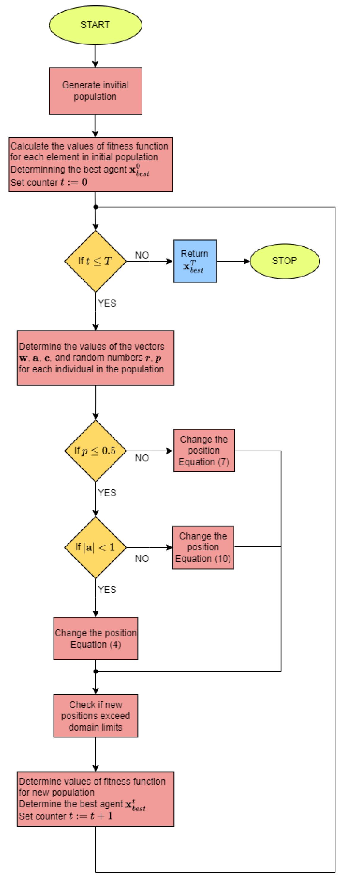
3.1. Whale Optimization Algorithm

This section describes the Whale Optimization Algorithm (WOA), which is used to solve the considered optimization problem. The inspiration for this algorithm is the behavior of whales when searching for prey. The mechanism these mammals use when hunting for prey seems interesting and served as a background for the algorithm. In the literature, the hunting method of these animals is called the bubble-net feeding method. To put it simply, when hunting, whales first dive into the water and then move along a spiral path, circling the prey and creating bubbles. Then they use one of several techniques: coral loop, lobtail, and capture loop. This behavior has only been observed in humpback whales. Rules and principles governing the algorithm are presented next in this section.
  • In each of iteration (t is number of iteration), the best individual in the population x b e s t t is determined. This individual’s position is closest to the prey, and other individuals move towards it according to the following formulas
    d = | c x b e s t t x t | ,
    x t + 1 = x b e s t t a d ,
    where a , c are vectors of random coefficients, x t is an individual in population t, and  d is a scaled vector of distance between an individual x t and the best individual x b e s t t in the population. The operation ∗ means multiplying vectors element by element. Vectors a , c are calculated in following way
    a = 2 w r w ,
    c = 2 r ,
    where r is a vector of random numbers in the range [ 0 , 1 ] , and  w is a vector of numbers decreasing from iteration to iteration from 2 to 0. The values of the vector w in a fixed iteration t are assumed to be 2 T t T , where T is the maximum number of iterations. Decreasing the w parameter in each iteration simulates the process of narrowing the space to search for a victim. This technique is called shrinking encircling mechanism.
  • The next important stage is the mechanism of spiral-shaped movement of whales. Mathematically, we describe this process with the following formula
    x t + 1 = d e b r cos ( 2 π r ) + x b e s t t ,
    where d = | x b e s t t x t | is the distance vector between the current individual and the best individual in the population, b is a constant (parameter of the algorithm), and r is a random number in the range [ 1 , 1 ] .
  • Whales move using both a shrinking encircling mechanism and a spiral-shaped movement. In the algorithm, this behavior is simulated by the formula
    x t + 1 = x b e s t t a d Equation ( 4 ) , for p 0.5 , d e b r cos ( 2 π r ) + x b e s t t Equation ( 7 ) , for p > 0.5 .
    In the above formula p [ 0 , 1 ] , therefore, there is a 50 % chance of making each move. It is possible to control behavior of the algorithm by the level of probability p. Standard approach assumes a level of 0.5 .
  • During the exploration phase, whales behave similarly to in Equation (4), with the difference that for the vector a , we assume | a | > 1 , which simulates the exploration phase and the whales move along with a random individual in the population, not the best individual. This stage of the algorithm is described mathematically by the formulas
    d = | c x r a n d t x t | ,
    x t + 1 = x r a n d t a d ,
    where x r a n d t denotes the position of a random whale in the population t.
  • The vector w , whose values change from iteration to iteration in the range from 2 to 0, is responsible for the transition from the exploration phase to the exploitation phase. For values of the vector w in the range ( 1 , 2 ] , there is an exploration phase, while for the range [ 0 , 1 ] , there is an exploitation phase.
  • The way of decreasing the value of the vector w in the Formula (5) and the level of probability appearing in the Formula (8) are tuning parameters of the WOA and can take different values.
Algorithm 1 presents the following steps of the WOA algorithm. Details about the described algorithm, as well as its application to selected problems, can be found in the articles [41,42,43].
Algorithm 1: Pseudocode of WOA
Symmetry 16 00233 i001
Figure 1 presents the block diagram of WOA.

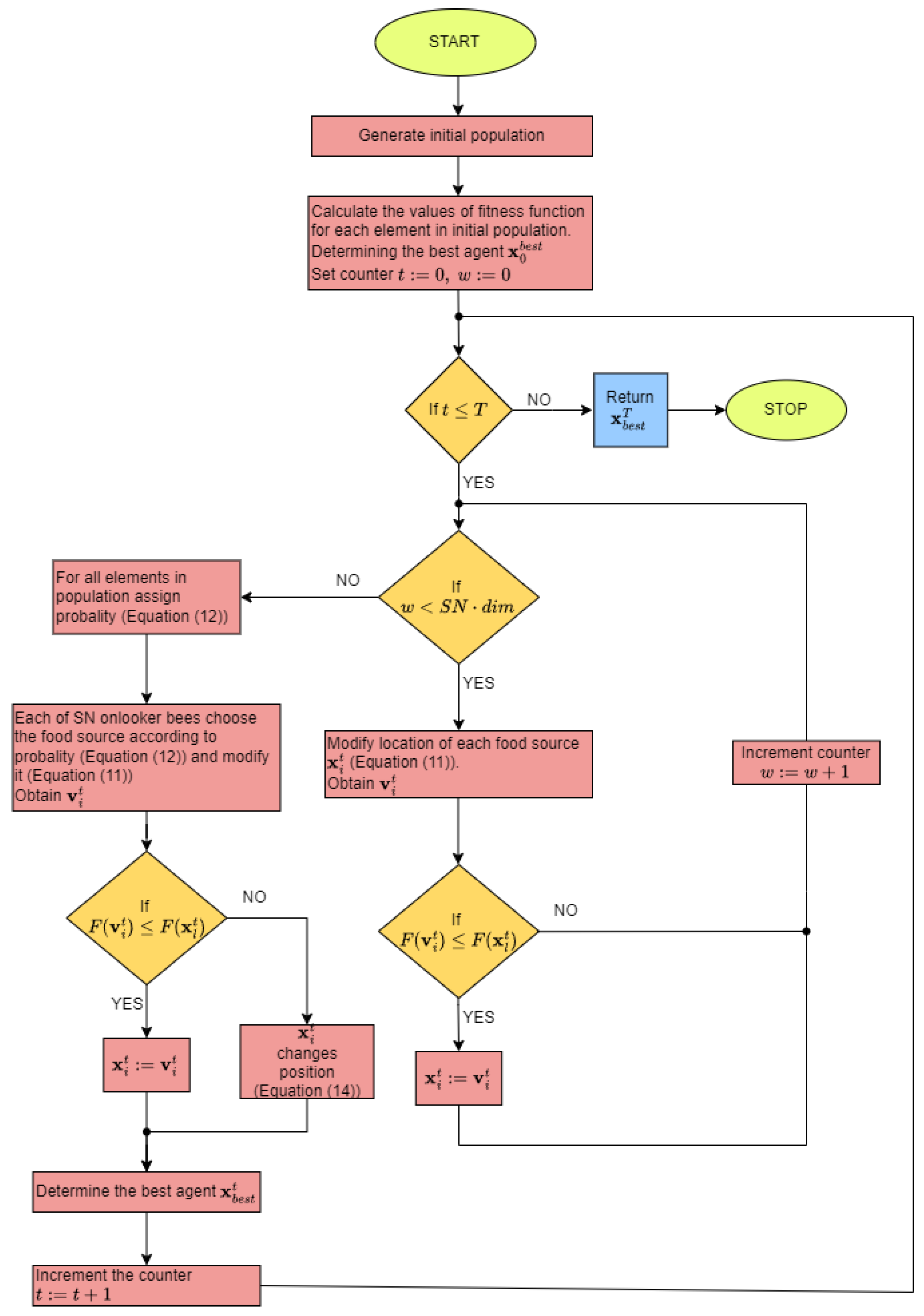
3.2. Artificial Bee Colony

The Artificial Bee Colony (ABC) optimization algorithm draws its inspiration from the behavior of bees. This subsection is devoted to the mathematical description of the ABC algorithm.
Bees looking for a food source can be divided into two groups
  • working bees—these are bees whose job is to look for a food source. Important information for these bees consists of the following: the distance between the hive and the food source, the direction the bee should follow to reach the food source and the amount of nectar in the source.
  • bees unclassified—these are bees that search for new food sources. We can divide them into two groups: scouts and onlookers. Scouts, after leaving a food source, look for another one in randomly way, while viewers look for visited sources based on the information provided.
Bees communicate with each other to exchange information about their food source through dancing. Unclassified bees belonging to the onlookers group can choose the most relevant food source by observing the dance. Once a bee locates a food, it remembers its location and immediately starts exploring it. After obtaining a sufficient amount of nectar, it returns to the hive and unloads the collected food. Then it is faced with choosing one of three options:
  • abandons the source, becomes an onlooker and watches the bees conveying information,
  • transmits information through dance and recruits other bees,
  • continues to explore on its own, without hiring other bees.
Based on the above assumptions, the bee algorithm was created, the main assumptions of which are as follows
  • the locations of food sources correspond to potential solutions of the optimized problem.
  • the quantity of nectar in the source corresponds to the quality of the solution.
  • the number of working bees is equal to the number of onlookers, which is denoted by SN.
  • Food sources are modified according to the formula
    v i t = x i t + r ( x i t x k t ) ,
    where k { 1 , 2 , , S N } k i is the random index, r is a vector of randomly generated numbers in the range [ 1 , 1 ] , the operation ∗ means multiplying the vector “element by element”, x i t denotes i-th solution from the population in the t-th iteration and v i t denotes i-th the modified solution from the population in the t-th iteration.
    Compare positions v i t with   x i t . If  F ( v i t ) F ( x i t ) . The position of x i t in the population t is then replaced by v i t . Otherwise, the position x i t remains in the population.
  • Each item in population is assigned a probability according to the formula
    p i = f i t ( x i ) j = 1 S N f i t ( x j ) , i = 1 , 2 , , S N ,
    where
    f i t ( x i ) = 1 1 + F ( x i ) , if F ( x i ) 0 , 1 + | F ( x i ) | , if F ( x i ) < 0 .
  • Each onlooker bee selects one source according to the probability p i and starts searching near it according to the Formula (11). Then the bee compares two locations—the new and previous one.
  • If, after performing the previous step of the algorithm, any of the food sources have not changed their position, then they are omitted and replaced with a new random source
    x i = x min + r ( x max x min ) , i = 1 , 2 , , S N ,
    where r is a vector of random numbers in the range [ 0 , 1 ] , and  x min , x max are vectors of constraints, respectively lower and upper limits of the search space domain.
Algorithm 2 shows the following steps of the ABC method. More about this algorithm and its applications can be found in [44].
Algorithm 2: Pseudocode of ABC
Symmetry 16 00233 i002
Figure 2 presents the block diagram of the ABC algorithm.

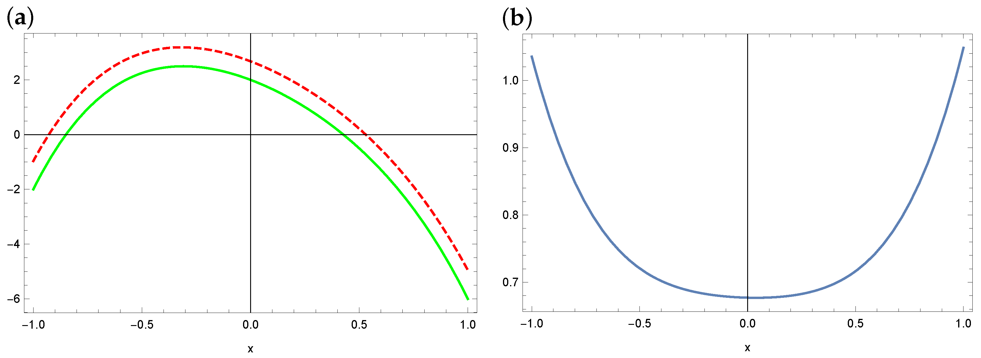
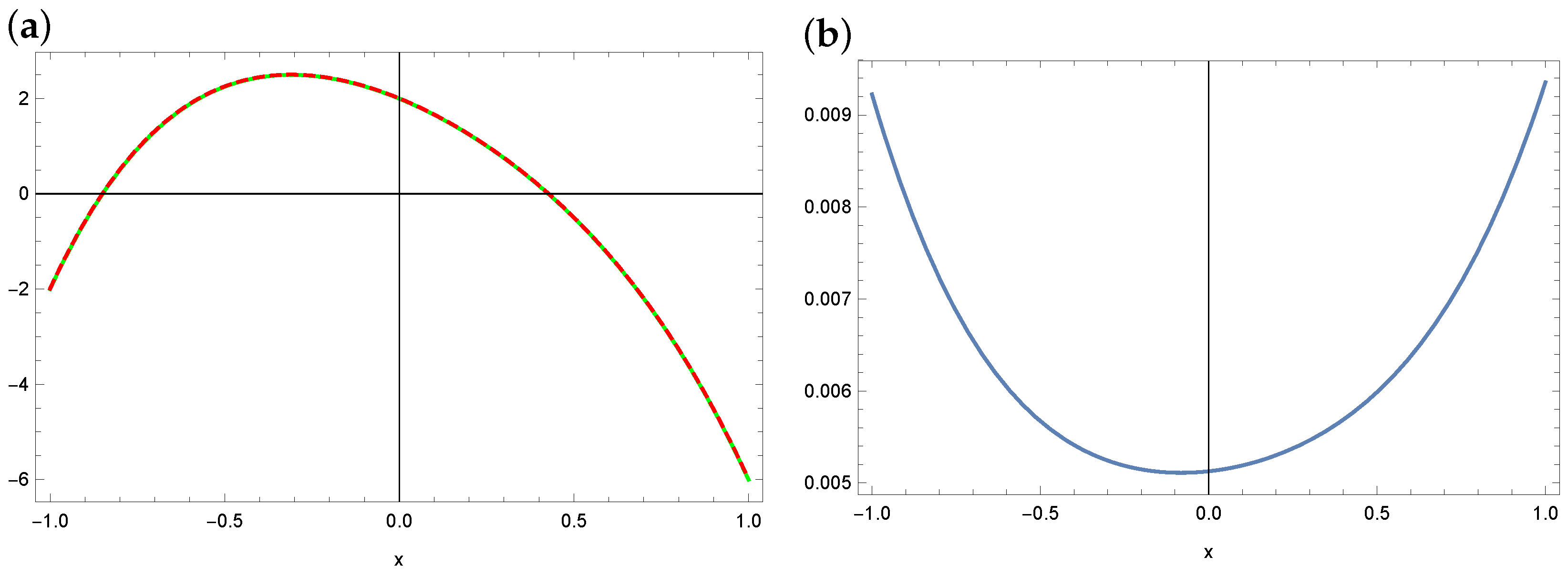
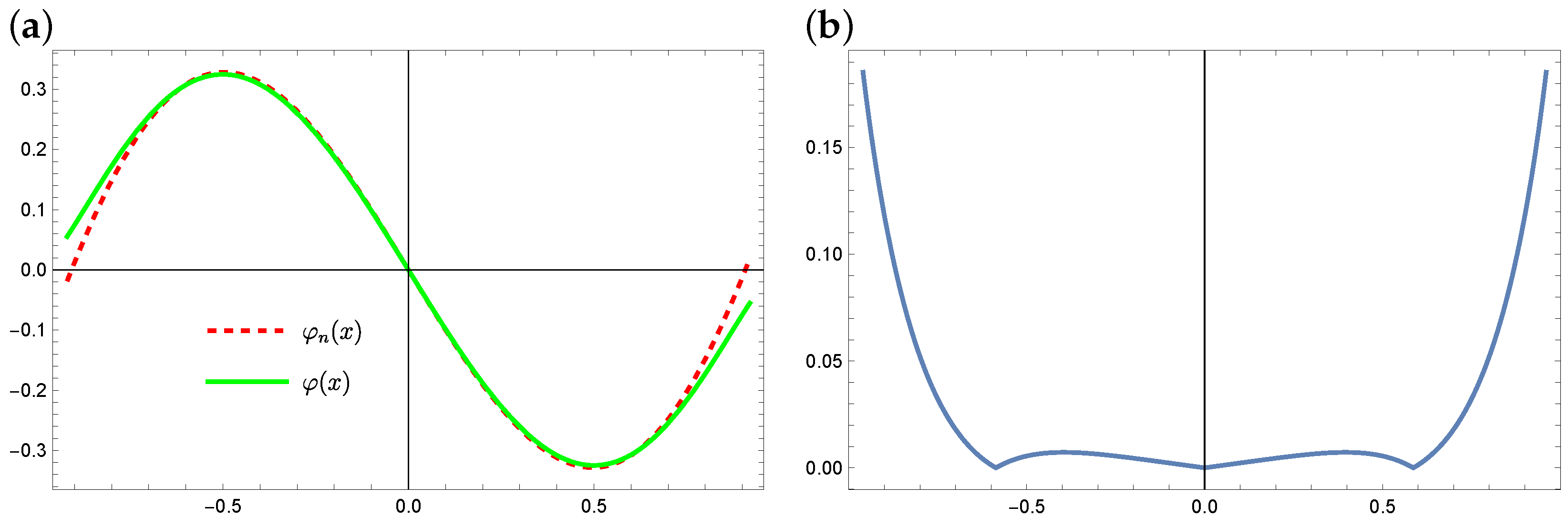
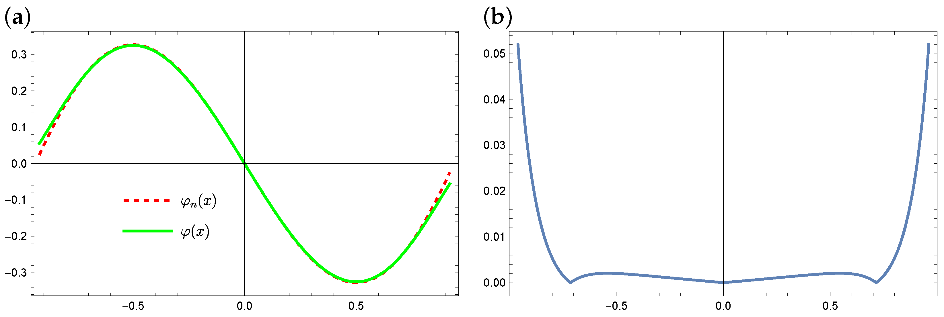
4. Numerical Examples

This section presents computational examples illustrating the effectiveness of the methods described in this paper. The considered algorithms were compared with each other.

4.1. Example 1

Let us consider the equation
2 φ ( x ) + 1 1 φ ( t ) t x d t = x 2 ,
which is considered important in the scientific literature (see, e.g., [39]), due to its occurrence in works related to heat conduction and radiation research.
Since we do not know the analytical (exact) solution to this problem, we plot absolute error Δ ( x ) based on the obtained approximate solution
Δ ( x ) = 2 φ n ( x ) + λ 1 1 φ n ( t ) t x d t f ( x ) ,
which, in this case, comes down to the following form
Δ ( x ) = 2 φ n ( x ) + x 2 + 1 1 φ n ( t ) t x d t .
Figure 3 presents the errors of the solution obtained from the method using the Taylor series and for different values of the number of terms n: for n = 8 , left side and for n = 10 , right side.
The error curves in both cases are similar in nature, i.e., the highest error values are achieved at the edges of the interval. Taking n = 10 reduces the size of the error by one order compared to n = 8 .
Now, we present a solution to this example by using the WOA and ABC algorithms. Since we do not know the exact solution, an approximate solution was adopted in the form of polynomials of degree 3, 4 and 5. Figure 4, Figure 5 and Figure 6 show the distribution of errors in the approximate solution for WOA and ABC. For example Figure 5 shows the distribution of errors in the case of a fourth-degree polynomial. As we can see in Figure 5, smaller errors were obtained in the case of the WOA solution. The highest errors are obtained in the case of ABC, but they are also at a satisfactory level. In the case of polynomials of degree 3 and 5, analogous error graphs are included in Figure 4 and Figure 6.

4.2. Example 2

Let us consider equation
2 φ ( x ) + 1 1 φ ( t ) t x d t = f ( x ) ,
where λ = 1 ,
f ( x ) = 2 3 ( 17 + 38 x 12 x 2 + 30 x 3 ) + ( 2 3 x 4 x 2 + x 3 2 x 4 ) ln 1 x 1 + x .
Exact solution for this problem has following form
φ ( x ) = 2 3 x 4 x 2 + x 3 2 x 4 .
Since we know the exact solution, we do not need to check the accuracy of the approximate solution using (15). In this case, the absolute error Δ n is defined more simply
Δ n ( x ) = φ ( x ) φ n ( x ) .
First, the Taylor series method was used to solve the equation. The plots of the exact solution φ and the approximate solution φ n and the errors of these approximations are provided in Figure 7 (for n = 4 ) and Figure 8 (for n = 6 ). As we can see, only for n = 6 , the errors of the obtained solution are minimal, approximately 10 15 . In the case of n = 4 , the approximate solution maintains properties of the exact solution, but the differences between the two functions are significant.
Now, we discuss the obtained solutions when using ABC and WOA algorithms. It is assumed that the form of the sought function would be a polynomial of the fourth degree, i.e., φ ¯ ( x ) = a 0 + a 1 x + a 2 x 2 + a 3 x 3 + a 4 x 4 . Therefore, five coefficients are sought: a 0 , a 1 , , a 4 . As a result of using the metaheuristic algorithms, the following results were obtained (see Table 1). As we can see, the value of the fitness function F in the case of ABC is much smaller than in the case of WOA. This proves that the ABC algorithm works better for this example, which is especially visible when comparing results of finding parameters a 0 and a 4 . The exact values of these coefficients are 2 and 2 , respectively. WOA returned values of a 0 2.67 , a 4 1.73 , while ABC returned a 0 2.00 , a 4 1.99 . Figure 9 and Figure 10 present the solutions found by WOA and ABC, respectively, compared with the exact solution, along with the distribution of errors in the domain. It is clear that ABC solves the problem very well, while the result obtained from WOA is not so good.

4.3. Example 3

In this example, we again consider the following equation
2 φ ( x ) + 1 1 φ ( t ) t x d t = f ( x ) ,
where function f has the form
f ( x ) = 2 4 x 4 5 x 2 + 1 1 x 2 1 8 π 8 x 4 12 x 2 + 3 .
The exact solution to this problem is a function
φ ( x ) = x ( x 2 1 ) 1 x 2 .
As in the case of the previous examples, the solution is sought in the form of a polynomial. To estimate the absolute errors Formula (16) was used.
Plots of the exact solution φ and the approximate solution φ n and the errors of these approximations (for the method with Taylor series expansion) are presented in Figure 11 (for n = 6 ), and Figure 12 (for n = 16 ). We can notice that inside the considered area the approximation, errors are minimal and when closing to the ends of interval [ 1 , 1 ] , these errors increase slightly.
We now present solutions obtained using metaheuristic optimization algorithms. The solution is sought in the form
ϕ ¯ ( x ) = i = 0 n a i x i .
In the case of metaheristic algorithms, it is assumed n = 3 , 4 , 5 . As can be seen in the Figure 13, Figure 14, Figure 15, Figure 16, Figure 17 and Figure 18, in the case of metaheuristic algorithms, the best results are obtained for the ABC algorithm and the n = 3 case. Definitely, worse results are obtained in the case of WOA.

5. Conclusions

In the article, two different approaches for solving the integro-differential equation with the Cauchy kernel were compared. The first method used Taylor series expansion of functions, and the second group consists of two selected metaheuristic optimization algorithms—the classic ABC algorithm and the younger WOA algorithm. Both are used in recent papers in many problems.
Numerical examples show that both methods are effective in solving this important and difficult task. For this purpose, three numerical examples of varying complexity were presented, both for equations in which we know the exact solution and for those where such a solution is not known. The research has shown that the first of the discussed methods works better with solving the considered type of equation and generates noticeably smaller errors. Heuristic methods also solve this type of task.
To sum up, we can say that the main advantages of the method based on the Taylor series is higher in accuracy than in case of the metaheuristic approach. A slight disadvantage of this method is the specific form of the system of equations being solved, which may be indeterminate for certain degrees of the sought polynomial. However, the main advantages of metaheuristic methods are their universality. Once the method has been implemented, the form of the equation being solved does not affect the difficulty of adopting it to the algorithm. It only requires specifying the class of functions (e.g., polynomials) in which the solution will be sought. Then, an error function is constructed that depends on the coefficients of the function being sought. By finding the minimum of the error function, we obtain an approximate solution. The disadvantages of these methods include the total running time. In order to effectively search for solutions, it is necessary to spend time in advance to ’tune’ the algorithm parameters. We also obtained errors in the approximate solution that were higher than in the case of the method with the Taylor series. But in many engineering problems, the obtained solution is sufficiently satisfactory.
It should be mentioned here that thanks to the symmetric domain and the appropriate form of the f function, certain conclusions can be drawn in some cases. For example, in example 1, the given function f is even (its graph is symmetrical about the Y axis), so we can expect that the solution will be an odd function (its graph is symmetrical about the origin), and in example 3, we have the opposite situation—the graph of the f function is symmetrical with respect to the origin of the coordinate system, so it is probable that the graph of the sought function φ will be symmetrical with respect to the Y axis. In both cases, this assumption turned out to be true, and the correct assumption of the truth of the hypothesis about the form of the function φ can significantly shorten the time of searching for this function and improve the quality of the solution.
Our future research plans focus on exploring a broader class of meta-heuristic algorithms. Another idea is to take into account hybrid methods, i.e., combining a heuristic method with a certain deterministic method (e.g., Nelder–Mead or Hooke–Jeeves). We also plan to generalize the class of the considered integro-differential equation.

Author Contributions

Conceptualization, M.P. and R.B.; methodology, M.P.; software, M.P. and R.B.; validation, M.P. and R.B.; formal analysis, R.B.; writing—original draft preparation, M.P. and R.B.; writing—review and editing, M.P. and R.B. All authors have read and agreed to the published version of the manuscript.

Funding

This research received no external funding.

Data Availability Statement

Data are contained within the article.

Conflicts of Interest

The authors declare no conflict of interest.

References

  1. Alexandrov, V.M.; Kovalenko, E.V. Problems with Mixed Boundary Conditions in Continuum Mechanics; Science: Moscow, Russia, 1986. [Google Scholar]
  2. Frankel, J. A Galerkin solution to a regularized Cauchy singular integro-differential equation. Q. Appl. Math. 1995, 53, 245–258. [Google Scholar] [CrossRef]
  3. Hori, M.; Nasser, N. Asymptotic solution of a class of strongly singular integral equations. SIAM J. Appl. Math. 1990, 50, 716–725. [Google Scholar] [CrossRef]
  4. Koya, A.C.; Erdogan, F. On the solution of integral equations with strongly singular kernels. Q. Appl. Math. 1987, 45, 105–122. [Google Scholar] [CrossRef]
  5. Jäntschi, L. Modelling of acids and bases revisited. Stud. UBB Chem. 2022, 67, 73–92. [Google Scholar] [CrossRef]
  6. Hochstadt, H. Integral Equations; Wiley Interscience: New York, NY, USA, 1973. [Google Scholar]
  7. Muskelishvili, N.I. Singular Integral Equations; Noordhoff: Groningen, The Netherlands, 1953. [Google Scholar]
  8. Tricomi, F.G. Integral Equations; Dover: New York, NY, USA, 1985. [Google Scholar]
  9. Atkinson, K.E. A Survey of Numerical Methods for the Solution of Fredholm Integral Equations of the Second Kind. J. Integral Equ. Appl. 1992, 4, 15–46. [Google Scholar] [CrossRef]
  10. Badr, A.A. Integro-differential equation with Cauchy kernel. J. Comput. Appl. Math. 2001, 134, 191–199. [Google Scholar] [CrossRef]
  11. Bhattacharya, S.; Mandal, B.N. Numerical solution of a singular integro-differential equation. Appl. Math. Comput. 2008, 195, 346–350. [Google Scholar] [CrossRef]
  12. Delves, L.M.; Mohamed, J.L. Computational Methods for Integral Equations; Cambridge University Press: London, UK, 2008. [Google Scholar] [CrossRef]
  13. Linz, P. Analytical and Numerical Methods for Volterra Equations; SIAM: Philadelphia, PA, USA, 1987. [Google Scholar]
  14. Maleknejad, K.; Arzhang, A. Numerical solution of the Fredholm singular integro-differential equation with Cauchy kernel by using Taylor-series expansion and Galerkin method. Appl. Math. Comput. 2006, 182, 888–897. [Google Scholar] [CrossRef]
  15. Mennouni, A. A projection method for solving Cauchy singular integro-differential equations. Appl. Math. Lett. 2012, 25, 986–989. [Google Scholar] [CrossRef]
  16. Tunç, O.; Tunç, C.; Yao, J.-C.; Wen, C.-F. New Fundamental Results on the Continuous and Discrete Integro-Differential Equations. Mathematics 2022, 10, 1377. [Google Scholar] [CrossRef]
  17. Tunç, C.; Tunç, O.; Yao, J.-C. On the Enhanced New Qualitative Results of Nonlinear Integro-Differential Equations. Symmetry 2023, 15, 109. [Google Scholar] [CrossRef]
  18. Pavlycheva, N.; Niyazgulyyewa, A.; Sachabutdinow, A.; Anfinogentow, V.; Morozow, O.; Agliullin, T.; Valeev, B. Hi-Accuracy Method for Spectrum Shift Determination. Fibers 2023, 11, 60. [Google Scholar] [CrossRef]
  19. Kukushkin, M.V. Cauchy Problem for an Abstract Evolution Equation of Fractional Order. Fractal Fract. 2023, 7, 111. [Google Scholar] [CrossRef]
  20. Chen, L.; Li, J.; Li, Y.; Zhao, Q. Even-Order Taylor Approximation-Based Feature Refinement and Dynamic Aggregation Model for Video Object Detection. Electronics 2023, 12, 4305. [Google Scholar] [CrossRef]
  21. Qiao, J.; Yang, S.; Zhao, J.; Li, H.; Fan, Y. A Quantitative Study on the Impact of China’s Dual Credit Policy on the Development of New Energy Industry Based on Taylor Expansion Description and Cross-Entropy Theory. World Electr. Veh. J. 2023, 14, 295. [Google Scholar] [CrossRef]
  22. La, V.N.T.; Minh, D.D.L. Bayesian Regression Quantifies Uncertainty of Binding Parameters from Isothermal Titration Calorimetry More Accurately Than Error Propagation. Int. J. Mol. Sci. 2023, 24, 15074. [Google Scholar] [CrossRef] [PubMed]
  23. Bayram, H.; Vijaya, K.; Murugusundaramoorthy, G.; Yalçın, S. Bi-Univalent Functions Based on Binomial Series-Type Convolution Operator Related with Telephone Numbers. Axioms 2023, 12, 951. [Google Scholar] [CrossRef]
  24. Haupin, R.J.; Hou, G.J.-W. A Unit-Load Approach for Reliability-Based Design Optimization of Linear Structures under Random Loads and Boundary Conditions. Designs 2023, 7, 96. [Google Scholar] [CrossRef]
  25. Liu, Y.; Duan, C.; Liu, L.; Cao, L. Discrete-Time Incremental Backstepping Control with Extended Kalman Filter for UAVs. Electronics 2023, 12, 3079. [Google Scholar] [CrossRef]
  26. Zhang, J.; Xiao, G.; Deng, G.; Zhang, Y.; Zhou, J. The Quadratic Constitutive Model Based on Partial Derivative and Taylor Series of Ti6242s Alloy and Predictability Analysis. Materials 2023, 16, 2928. [Google Scholar] [CrossRef]
  27. Brociek, R.; Chmielowska, A.; Słota, D. Comparison of the probabilistic ant colony optimization algorithm and some iteration method in application for solving the inverse problem on model with the caputo type fractional derivative. Entropy 2020, 22, 555. [Google Scholar] [CrossRef]
  28. Dai, Y.; Yu, J.; Zhang, C.; Zhan, B.; Zheng, X. A novel whale optimization algorithm of path planning strategy for mobile robots. Appl. Intell. 2023, 53, 10843–10857. [Google Scholar] [CrossRef]
  29. Rana, N.; Latiff, M.S.A.; Abdulhamid, S.M.; Chiroma, H. Whale optimization algorithm: A systematic review of contemporary applications, modifications and developments. Neural Comput. Appl. 2020, 32, 16245–16277. [Google Scholar] [CrossRef]
  30. Brociek, R.; Pleszczyński, M.; Zielonka, A.; Wajda, A.; Coco, S.; Lo Sciuto, G.; Napoli, C. Application of heuristic algorithms in the tomography problem for pre-mining anomaly detection in coal seams. Sensors 2022, 22, 7297. [Google Scholar] [CrossRef]
  31. Rahnema, N.; Gharehchopogh, F.S. An improved artificial bee colony algorithm based on whale optimization algorithm for data clustering. Multimed. Tools Appl. 2020, 79, 32169–32194. [Google Scholar] [CrossRef]
  32. Kaya, E. A New Neural Network Training Algorithm Based on Artificial Bee Colony Algorithm for Nonlinear System Identification. Mathematics 2022, 10, 3487. [Google Scholar] [CrossRef]
  33. Brociek, R.; Słota, D. Application of real ant colony optimization algorithm to solve space fractional heat conduction inverse problem. Commun. Comput. Inf. Sci. 2016, 639, 369–379. [Google Scholar] [CrossRef]
  34. Bacanin, N.; Stoean, C.; Zivkovic, M.; Jovanovic, D.; Antonijevic, M.; Mladenovic, D. Multi-Swarm Algorithm for Extreme Learning Machine Optimization. Sensors 2022, 22, 4204. [Google Scholar] [CrossRef]
  35. Jin, H.; Jiang, C.; Lv, S. A Hybrid Whale Optimization Algorithm for Quality of Service-Aware Manufacturing Cloud Service Composition. Symmetry 2024, 16, 46. [Google Scholar] [CrossRef]
  36. Tian, Y.; Yue, X.; Zhu, J. Coarse–Fine Registration of Point Cloud Based on New Improved Whale Optimization Algorithm and Iterative Closest Point Algorithm. Symmetry 2023, 15, 2128. [Google Scholar] [CrossRef]
  37. Li, M.; Xiong, H.; Lei, D. An Artificial Bee Colony with Adaptive Competition for the Unrelated Parallel Machine Scheduling Problem with Additional Resources and Maintenance. Symmetry 2022, 14, 1380. [Google Scholar] [CrossRef]
  38. Kaya, E.; Baştemur Kaya, C. A Novel Neural Network Training Algorithm for the Identification of Nonlinear Static Systems: Artificial Bee Colony Algorithm Based on Effective Scout Bee Stage. Symmetry 2021, 13, 419. [Google Scholar] [CrossRef]
  39. Mandal, B.N.; Bera, G.H. Approximate solution of a class of singular integral equations of second kind. J. Comput. Appl. Math. 2007, 206, 189–195. [Google Scholar] [CrossRef]
  40. Akay, B.; Karaboga, D. A survey on the applications of artificial bee colony in signal, image, and video processing. Signal Image Video Process. 2015, 9, 967–990. [Google Scholar] [CrossRef]
  41. Pham, Q.; Mirjalili, S.; Kumar, N.; Alazab, M.; Hwang, W. Whale Optimization Algorithm with Applications to Resource Allocation in Wireless Networks. IEEE Trans. Veh. Technol. 2020, 69, 4285–4297. [Google Scholar] [CrossRef]
  42. Mirjalili, S.; Lewis, A. The Whale Optimization Algorithm. Adv. Eng. Softw. 2016, 95, 51–67. [Google Scholar] [CrossRef]
  43. Sun, G.; Shang, Y.; Zhang, R. An Efficient and Robust Improved Whale Optimization Algorithm for Large Scale Global Optimization Problems. Electronics 2022, 11, 1475. [Google Scholar] [CrossRef]
  44. Du, H.; Liu, P.; Cui, Q.; Ma, X.; Wang, H. PID Controller Parameter Optimized by Reformative Artificial Bee Colony Algorithm. J. Math. 2022, 2022, 3826702. [Google Scholar] [CrossRef]
Figure 1. Block diagram of Whale Optimization Algorithm.
Symmetry 16 00233 g001
Figure 2. Block diagram of Artificial Bee Colony algorithm.
Symmetry 16 00233 g002
Figure 3. Plot of absolute errors Δ ( x ) for n = 8 (a) and n = 10 (b) (example 1).
Symmetry 16 00233 g003
Figure 4. Absolute error Δ ( x ) plot for a polynomial of degree 3 and the WOA (a) and ABC (b) algorithm (example 1).
Symmetry 16 00233 g004
Figure 5. Absolute error Δ ( x ) plot for a polynomial of degree 4 and the WOA (a) and ABC (b) algorithm (example 1).
Symmetry 16 00233 g005
Figure 6. Absolute error Δ ( x ) plot for a polynomial of degree 5 and the WOA (a) and ABC (b) algorithm (example 1).
Symmetry 16 00233 g006
Figure 7. The exact solution (solid green line) and approximate solution (dashed red line) for n = 4 (a) and the absolute errors Δ of this approximation (b) (example 2).
Symmetry 16 00233 g007
Figure 8. The exact solution (solid green line) and approximate solution (dashed red line) for n = 6 (a) and the absolute errors Δ of this approximation (b) (example 2).
Symmetry 16 00233 g008
Figure 9. The exact solution (solid green line) and approximate solution (dashed red line) in the case of WOA (a) and the absolute errors Δ of this approximation (b) (example 2).
Symmetry 16 00233 g009
Figure 10. The exact solution (solid green line) and approximate solution (dashed red line) in the case of ABC (a) and the absolute errors Δ of this approximation (b) (example 2).
Symmetry 16 00233 g010
Figure 11. The exact solution (solid green line) and approximate solution (dashed red line) for n = 6 (a) and the absolute errors Δ of this approximation (b) (example 3).
Symmetry 16 00233 g011
Figure 12. The exact solution (solid green line) and approximate solution (dashed red line) for n = 16 (a) and the absolute errors Δ of this approximation (b) (example 3).
Symmetry 16 00233 g012
Figure 13. The exact solution (solid green line) and approximate solution (dashed red line) for a polynomial of degree 3 (a) and the absolute errors Δ of this approximation in the case of WOA (b) (example 3).
Symmetry 16 00233 g013
Figure 14. The exact solution (solid green line) and approximate solution (dashed red line) for a polynomial of degree 3 (a) and the absolute errors Δ of this approximation in the case of ABC (b) (example 3).
Symmetry 16 00233 g014
Figure 15. The exact solution (solid green line) and approximate solution (dashed red line) for a polynomial of degree 4 (a) and the absolute errors Δ of this approximation in the case of WOA (b) (example 3).
Symmetry 16 00233 g015
Figure 16. The exact solution (solid green line) and approximate solution (dashed red line) for a polynomial of degree 4 (a) and the absolute errors Δ of this approximation in the case of ABC (b) (example 3).
Symmetry 16 00233 g016
Figure 17. The exact solution (solid green line) and approximate solution (dashed red line) for a polynomial of degree 5 (a) and the absolute errors Δ of this approximation in the case of WOA (b) (example 3).
Symmetry 16 00233 g017
Figure 18. The exact solution (solid green line) and approximate solution (dashed red line) for a polynomial of degree 5 (a) and the absolute errors Δ of this approximation in the case of ABC (b) (example 3).
Symmetry 16 00233 g018
Table 1. Sought coefficient values obtained using WOA and ABC methods. a i ( i = 0 , 1 , 2 , 3 , 4 ) —obtained coefficient value, F —objective function value.
a 0 a 1 a 2 a 3 a 4 F
WOA 2.6771 3.0077 3.9007 1.0142 1.7346 0.1631
ABC 2.0051 2.9996 3.9976 0.9996 1.9981 0.0034
Disclaimer/Publisher’s Note: The statements, opinions and data contained in all publications are solely those of the individual author(s) and contributor(s) and not of MDPI and/or the editor(s). MDPI and/or the editor(s) disclaim responsibility for any injury to people or property resulting from any ideas, methods, instructions or products referred to in the content.

