Modifying Hellwig’s Method for Multi-Criteria Decision-Making with Mahalanobis Distance for Addressing Asymmetrical Relationships

Abstract

Hellwig’s method is a multi-criteria decision-making technique designed to facilitate the ranking of alternatives based on their proximity to the ideal solution. Typically, this approach calculates distances using the Euclidean norm, assuming implicitly that the considered criteria are independent. However, in real-world situations, the assumption of criteria independence is rarely met. The paper aims to propose an extension of Hellwig’s method by incorporating the Mahalanobis distance. Substituting the Euclidean distance with the Mahalanobis distance has proven to be effective in handling correlations among criteria, especially in the context of asymmetrical relationships between criteria. Subsequently, we investigate the impact of the Euclidean and Mahalanobis distance measures on the several variants of Hellwig procedures, analyzing examples based on various illustrative data with 10 alternatives and 4 criteria. Additionally, we examine the influence of three normalization formulas in Hellwig’s aggregation procedures. The investigation results indicate that both the distance measure and normalization formulas have some impact on the final rankings. The evaluation and ranking of alternatives using the Euclidean distance measure are influenced by the normalization formula, albeit to a limited extent. In contrast, the Mahalanobis distance-based Hellwig’s method remains unaffected by the choice of normalization formulas. The study concludes that the ranking of alternatives is strongly dependent on the distance measure employed, whether it is Euclidean or Mahalanobis. The Mahalanobis distance-based Hellwig method is deemed a valuable tool for decision-makers in real-life situations. It enables the evaluation of alternatives by considering interactions between criteria, providing a more comprehensive perspective for decision-making.

1. Introduction

Multi-criteria decision-making (MCDM) methods are a collection of techniques designed to address complex problems that involve the evaluation and ranking of alternatives based on multiple criteria, which may sometimes conflict with each other [1,2]. These methods are widely used in various fields [3], including business [4], engineering [5], environmental science [6], sustainability [7], and public policy [8], among others. The goal is to provide decision-makers with a systematic and structured approach to making choices when faced with a range of alternatives. Among them, there is a class of techniques based on aggregation formulas incorporating reference solutions, such as TOPSIS (Technique for Ordering Preferences by Similarity to Ideal Solution) [9], Hellwig’s method [10], VIKOR (VlseKriterijuska Optimizacija I Komoromisno Resenje) [11], DAPR [12], BWM (the Best-Worst Method) [13], or BIPOLAR [14].

MCDM methods typically involve several steps to determine the overall preference value for each alternative, as follows:

• Normalization: This step involves transforming performance ratings into a standardized unit scale.
• Weights determination: This process involves assigning weights to the criteria based on their relative importance in the decision-making process.
• Distance Measure: This step calculates the distance between the alternatives and reference points, providing a measure of their dissimilarity or similarity.
• Aggregation Formula: Aggregation involves combining the normalized values, weights, and distance measures to obtain an overall preference value for each alternative.

The paper focuses on Hellwig’s method [10] based on the measurement distances from the alternative to the ideal solution. Two critical aspects of this method have been scrutinized: the distance measure and normalization formula.

The aims of the paper are twofold. Firstly, it introduces an extension of Hellwig’s method, namely the Mahalanobis distance-based Hellwig method (HM). The classical Hellwig method (H) relies on Euclidean distance, assuming implicitly that the criteria are independent. However, real-life situations may not always align with this assumption. Therefore, it is necessary to adapt the technique to the new situation. The Mahalanobis distance is employed to measure the distance between the ideal and alternatives, taking into consideration the dependence among criteria. While the Euclidean distance presupposes independence among variables, the Mahalanobis distance considers the covariance structure, making it more appropriate for datasets with correlated or asymmetrically distributed variables.

Secondly, we specifically investigate the impact of the distance measure (Euclidean vs. Mahalanobis) and the normalization formula in Hellwig’s measure. Various normalization methods have been proposed in the literature [1,9,15] that can be employed within MCDM. The article by Jahan and Edwards [15] undertakes a comparative analysis of six normalization techniques within multi-criteria decision-making methods. For our comparative analysis, we employed three well-known normalization procedures: vector normalization, linear scale transformation (Max-Min method), and linear scale transformation (Sum method).

Several authors have investigated how alternative normalization procedures can influence the ranking of alternatives obtained through MCDM methods [16,17,18,19,20,21,22,23]. We analyze and compare results derived from examples utilizing different variants of Hellwig’s method, taking into account two distance measures and three normalization formulas. This analysis is conducted using illustrative data comprising 10 alternatives and 4 criteria.

The rest of the paper is organized as follows: In Section 2, we briefly outline the concept of Mahalanobis distance and its application in multi-criteria analyses. In Section 3, the classical and extended Hellwig methods are presented. In Section 4, five illustrative examples are investigated concerning distance measures (Euclidean and Mahalanobis) and normalization formulas (vector normalization, min-max method, sum method) with differences in the dependence between criteria. The paper finishes with a conclusion.

2. Mahalanobis Distance and Multi-Criteria Analyses

The Mahalanobis distance, first proposed by Mahalanobis in 1936 [24], is a statistical metric for measuring distance with particular applicability in tasks such as classification, clustering, and multi-criteria decision-making. This distance is based on the separation between two points within a multi-dimensional space, based on the covariance among different variables. The covariance matrix incorporated in the distance measure calculation represents the interrelationships and interdependencies among variables. When the covariance matrix is equal to the identity matrix, the Mahalanobis distance simplifies to the Euclidean distance. The more precise description, calculation, and comparison of Euclidean distance and Mahalanobis distance can be found in [25]. Studies [26,27,28,29] are devoted to the Mahalanobis distance and its properties in the context of multicriteria analysis.

Multi-criteria methods based on Mahalanobis and Euclidean distances find widespread application in data analysis. The Mahalanobis distance finds utility in several MCDM approaches, including TOPSIS [26,27,28,29,30,31], TODIM (an acronym in Portuguese for Interactive and Multicriteria Decision Making) [32], or other decision-making problems [33,34,35,36]. The Mahalanobis distance, incorporating correlations with diverse criteria, empowers us to proficiently address the asymmetrical relationships among criteria. It aids decision-makers in evaluating alternatives based on their preferences and goals, taking into account the interaction between criteria.

3. Mahalanobis Distance-Based Hellwig Method

3.1. The Hellwig’s Framework—A Short Literature Review

Hellwig’s method [10], originally proposed by Hellwig in 1968, has undergone several modifications to address real-life problems. In his pioneering work [10], Hellwig introduced the concept of the development measure based on the pattern of economic development based on the most favorable values for each criterion. This method allows for determining the ranking of objects described in the multidimensional space by calculating the distances between the pattern of development and the objects. This concept has been applied to assess differences and similarities among various countries regarding qualified staff, corresponding to the economic development level of each country.

Hellwig’s method is particularly popular as a linear ordering technique in Polish literature, especially in the field of economic research. It is worth noting that the number of citations has been steadily increasing, particularly due to numerous publications in English. It has also gained recognition among international researchers as a multi-criteria method based on a reference point. According to Google Scholar (Harzing’s Publish or Perish 8 software as of 1 January 2024), the paper [10] has been cited 1479 times (26.41 times per year).

Hellwig’s method has been extended to address different problems with crisp data [10] and incorporates fuzzy sets [10], intuitionistic fuzzy sets [37,38,39,40], interval-valued fuzzy sets [41], and oriented fuzzy sets [42]. This method has been applied in various practical contexts, including the circular economy [43], quality of human capital in the EU countries [44], socio-economic region development [45,46,47,48], sustainable development [49,50], quality of life [38,39,42], evaluation negotiation offers [40,42], analysis agriculture development [51,52,53,54], competitive balance of the Italian Football League [55], innovation in UE countries [56], evaluation of theater activity in Poland [57], and selection of locations [58], among others.

3.2. The Hellwig’s Method

Let us assume that we have $m$ alternatives $A_1,A_2,\dots ,A_m$ and $n$ decision criteria $C_1,C_2,\dots ,C_n,$ where $x_{ij}$ denote the criteria value of $A_i$ on $C_j$($i=1,2,\dots ,m; j=1, 2,\dots ,n$).

The Hellwig’s general framework consists of the following steps:

Step 1. Determination of the decision matrix:

$$D=\left[x_{ij}\right],$$

(1)

where $x_{ij}$ is the value of the $j$-th criterion for $i$-th alternative $i=1,\dots ,m$, $j=1,\dots ,n.$

Step 2. Determination of the vector of weights:

$$w=\left[w_1,\dots ,w_n\right]$$

(2)

where $w_j>0\left(j=1,\dots ,n\right)$ is the weight of the criterion $C_j$ and ${\displaystyle \sum }_{j=1}^n{w}_j=1$.

In the later analyses, we implemented equal weights. However, it should be noted that in the literature, various proposals exist for establishing weights [59,60,61,62,63,64]. Tzeng et al. [65] classifies weighting methods as objective when weights are computed from outcomes and subjective when they depend only on the preferences of decision-makers. The third class is the combination of subjective and objective weighting methods. Da Silva et al. [62] identified and discussed more than 50 methods, of which 49 are subjective, 7 are objective, and others are hybrid.

Step 3. Building the ideal solution (pattern of development):

$$\mathrm{I}=\left[x_1^{+},\dots ,x_n^{+}\right]$$

(3)

where:

$$x_j^{+}=\{\begin{array}{c}\underset{i}{\max }{x}_{ij} \mathrm{for}\mathrm{benefit}\mathrm{criterion}\\ \underset{i}{\min }{x}_{ij} \mathrm{for}\cos \mathrm{t}\mathrm{criterion}.\end{array}$$

(4)

for $j=1,\dots ,n.$

Step 4. Determination of the normalized matrix:

$$\overline{D}=\left[{\overline{x}}_{ij}\right]$$

(5)

where ${\overline{x}}_{ij }$ is a normalized value of $x_{ij}$ ($i=1,\dots ,m$, $j=1,\dots ,n).$

We presented here three well-known and frequently used normalization techniques that we later applied for comparison studies [9,19,20]:

• Vector normalization, which transforms performance ratings into a normalized vector as follows:

$${\overline{x}}_{ij }=\frac{x_{ij}}{\sqrt{{{\displaystyle \sum }}_{i=1}^m{\left(x_{ij}\right)}^2}}$$

(6)

• Linear scale transformation (Max-Min method) which involves scaling the performance ratings linearly based on the minimum and maximum values observed across criteria.

$${\overline{x}}_{ij }=\frac{x_{ij}-\underset{i}{\min }{x}_{ij}}{\underset{i}{\max }{x}_{ij}-\underset{i}{\min }{x}_{ij}}$$

(7)

• Linear scale transformation (Sum method), where performance ratings are linearly transformed based on the sum of values across all criteria.

$${\overline{x}}_{ij }=\frac{x_{ij}}{{{\displaystyle \sum }}_{i=1}^m{x}_{ij}}$$

(8)

where $x_{ij}$ is the value of the $j$-th criterion for $i$-th alternative $i=1,\dots ,m$, $j=1,\dots ,n.$

Step 5. Building the weighted normalized matrix:

$$\tilde{D}=\left[{\tilde{x}}_{ij}\right],$$

(9)

where

$${\tilde{x}}_{ij}=w_j{\overline{x}}_{ij}$$

(10)

Step 6. Calculating the distances of $i$-th alternative $A_i$ from the ideal $I$ by using Euclidean or Mahalanobis distance measure

• Euclidean distance measure ($d{E}_i)$ [10]:

$$d{E}_i\left(A_i,\mathrm{I}\right)=\mathrm{E}\left({\tilde{A}}_i,\tilde{\mathrm{I}}\right)=\sqrt{{{\displaystyle \sum }}_{j=1}^n{\left({\tilde{x}}_{ij}-{\tilde{x}}_j^{+}\right)}^2}$$

(11)

where ${\tilde{x}}_{ij},{\tilde{x}}_j^{+}$ are weighted normalized values $x_{ij}$ and $x_j^{+}$, respectively.

• Mahalanobis distance measure ($d{M}_{i0})$ [29,31]:

$$d{M}_i\left(A_i,\mathrm{I}\right)=\mathrm{M}\left( {\overline{A}}_i,\overline{I}\right)=\sqrt{\left( {\overline{A}}_i-\overline{I}\right)W{C}^{-1}{W}^T{\left( {\overline{A}}_i-\overline{I}\right)}^T},$$

(12)

where C is the variance-covariance matrix of the data matrix $\overline{D},W=\mathrm{diag}(\sqrt{w_1},\dots ,\sqrt{w_n})$ is the diagonal matrix, where $w_1 ,w_2, . . . ,w_n$ are the weights assigned to the criteria.

In practical terms, the choice of distance measure depends on the data’s characteristics and the specifics of the multi-criteria analysis. While the Euclidean distance presupposes independence among variables, the Mahalanobis distance considers the covariance structure, making it more appropriate for datasets with correlated or asymmetrically distributed data. The Mahalanobis distance between the alternative and ideal solution is based on the normalized data and the estimated covariance matrix, which represents the relationships and dependencies between criteria.

Step 6. Calculating the Hellwig’s measure $H_{\mathrm{i}}$ or Hellwig’s measure based on Mahalanobis distance $H{M}_{\mathrm{i}}$ for the $i$-th alternative using the formula.

• Classical approach (H measure based on Euclidean distance):

$$H_i=1-\frac{d{E}_i}{d_0}$$

(13)

where $d_0=\overline{d}+2S,$ for $\overline{d}=\frac{1}{m}{\displaystyle \sum }_{i=1}^{m}d{E}_i$, $S=\sqrt{\frac{1}{m}{\displaystyle \sum }_{i=1}^m{(d{E}_i-\overline{d})}^2} .$

• Extended approach (HM measure based on Mahalanobis distance):

$$H{M}_i=1-\frac{d{M}_i}{d_0},$$

(14)

where $d_0=\overline{d}+2S,$ for $\overline{d}=\frac{1}{m}{\displaystyle \sum }_{i=1}^{m}d{M}_i$, $S=\sqrt{\frac{1}{m}{\displaystyle \sum }_{i=1}^m{(d{M}_i-\overline{d})}^2} .$

Step 7. Ranking of objects according to descending $H_i \mathrm{or} H{M}_i$ values.

A higher value of Hellwig’s measure corresponds to a higher ranking position for the respective alternative.

In the paper, Wang and Wang [31] showed the following:

Property 1: 

[31]: The non-singular linear transformation of data doesn’t affect the Mahalanobis distance measure.

Applying Property 1, and considering normalization Formulas (6)–(8) and Formula (14), we deduce the following:

Property 2: 

The Mahalanobis distance-based Hellwig method (HM) is independent of normalization formulas N1, N2, and N3.

4. Numerical Examples

This section compares the procedures and results obtained from the different Hellwig’s methods: the Hellwig method with Euclidean distance based on vector normalization (H1), max-min normalization (H2), and sum normalization (H3), and the Hellwig method with Mahalanobis distance (HM). Let us note that, from property 2, the results of HM methods don’t depend on the formalization formulas N1, N2, and N3. This gives us five variants of Hellwig’s method. The results of variants for Hellwig’s method were compared (a) based on Euclidean distance for different normalization formulas and (b) based on Euclidean distance with Mahalanobis distance measure.

The problem under consideration involves assessing ten alternatives with four benefit criteria. We assumed equal weight for the analyses to concentrate only on the distance measure and normalization formula incorporated in the algorithm. The examples differ in the data and correlations between criteria. To validate the HM method and examine the relationship between the criteria, we utilize the Pearson correlation coefficient. Additionally, the correlation between results obtained from different variants of Hellwig’s method is analyzed using both the Spearman and Pearson coefficients. The interpretation absolute value of the Pearson coefficient or Spearman coefficient is as follows: [0,0.1)—negligible; [0.1,0.40)—weak; [0.4, 0.7) moderate; [0.7,0.9) strong; [0.9,1] very strong.

Example 1. 

(negligible or weak correlation between criteria).

Table 1. Data and correlation matrix for Example 1.

Alternative	C1	C2	C3	C4			Correlation Matrix
A1	1	18	7	6			C1	C2	C3	C4
A2	3	2	10	10		C1	1.000	0.089	0.003	0.038
A3	5	30	15	30		C2	0.089	1.000	0.103	−0.003
A4	3	1	15	20		C3	0.003	0.103	1.000	0.116
A5	8	10	20	8		C4	0.038	−0.003	0.116	1.000
A6	2	20	10	5
A7	10	4	6	25
A8	12	25	10	2
A9	5	5	15	8
A10	6	2	5	9
Ideal solution	12	30	20	30

Legend: Absolute value of the Pearson coefficient.

[0,0.1)	[0.1,0.2)	[0.2,0.3)	[0.3,0.4)	[0.4,0.5)	[0.5,0.6)	[0.6,0.7)	[0.7,0.8)	[0.8,0.9)	[0.9,1.0)	1
negligible	weak			moderate			strong		very strong

displays the data and correlation matrix among the criteria in Example 1. In this case, a negligible or weak correlation is evident between the criteria. The highest Pearson correlation exists between criterion C3 and C4 (0.116), followed by C3 and C2 (0.103). All other Pearson coefficients are below 0.100.

The ideal based on max and min values (see Formula (3)) has the form:

$$I^{+}=\left[12,30,20,30\right].$$

The criteria values are normalized using Formulas (6)–(8), respectively. Following this, the Euclidean or Mahalanobis distances between the alternative and the ideal object are calculated using Formulas (11) or (12), respectively.

Finally, the synthetic measure is derived using Formula (13) or (14). The outcomes of various Hellwig’s measures are presented in Table 1.

From

Table 2. The distance values, measure values, and rank-ordering of alternatives obtained by different variants of Hellwig’s method (Example 1).

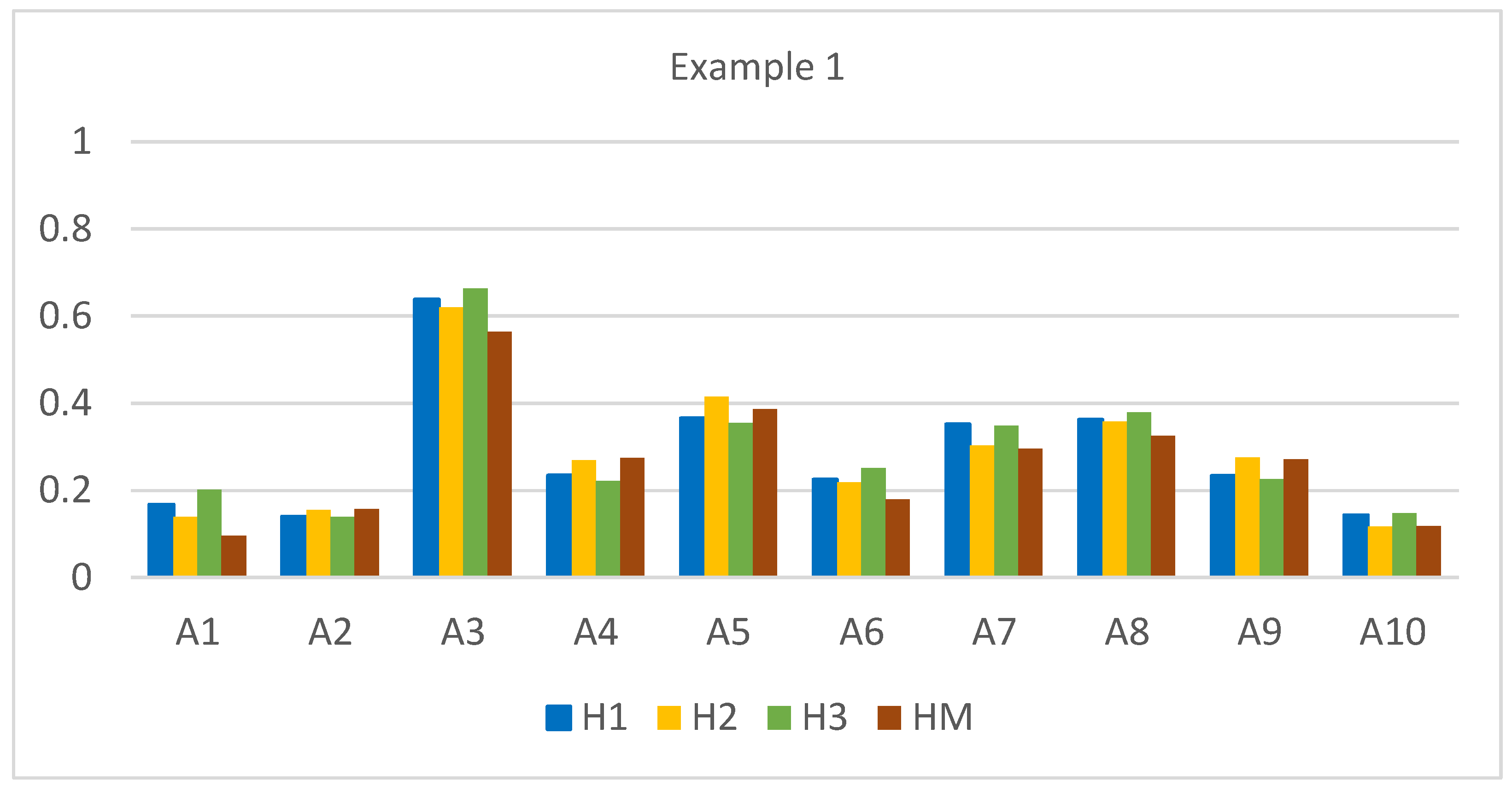
Alternative	dEH1	Value H1	Range H1	dEH2	Value H2	Range H2	dEH3	Value H3	Range H3	dM	Value HM	Range HM
A1	0.211	0.168	8	0.408	0.139	9	0.080	0.202	8	2.333	0.096	10
A2	0.218	0.141	10	0.400	0.155	8	0.086	0.140	10	2.177	0.157	8
A3	0.092	0.639	1	0.180	0.620	1	0.034	0.663	1	1.123	0.565	1
A4	0.194	0.235	5	0.345	0.270	6	0.078	0.222	7	1.872	0.275	5
A5	0.161	0.366	2	0.277	0.415	2	0.064	0.355	3	1.584	0.387	2
A6	0.197	0.225	7	0.370	0.219	7	0.075	0.252	5	2.116	0.180	7
A7	0.165	0.352	4	0.330	0.303	4	0.065	0.349	4	1.819	0.296	4
A8	0.162	0.363	3	0.304	0.358	3	0.062	0.380	2	1.741	0.326	3
A9	0.195	0.234	6	0.342	0.276	5	0.077	0.226	6	1.880	0.272	6
A10	0.217	0.144	9	0.418	0.117	10	0.085	0.148	9	2.277	0.118	9
do	0.254			0.473			0.100			2.582

, we can observe that rankings differ for Hellwig’s measures based on the Euclidean distance and various normalization formulas, but these differences are not so evident. Spearman coefficients between Hellwig’s measure based on Euclidean distance are the following: S(H1, H2) = 0.952, S(H1, H3) = 0.939, and S(H2, H3) = 0.915. The Pearson coefficient also confirms a very strong correlation: P(H1, H2) = 0.976, P(H1, H3) = 0.994, and P(H2, H3) = 0.956.

In all variants of Hellwig’s method, the rankings converge for alternatives A3 and A7. For the remaining alternatives, the disparity ranges only from 1 to 2 positions. Additionally, Spearman coefficients between the measure HM and other measures are very high: S(H1, HM) = 0.952, S(H2, HM) = 0.976, or high S(H3, HM) = 0.891. Similarly, a very strong correlation was observed when comparing those measures using the Pearson coefficient: P(H1, HM) = 0.956, P(H2, HM) = 0.991, and P(H3, HM) = 0.923. The highest concordance for HM is achieved with H2. The graphical representation results of Hellwig’s measures are illustrated in the accompanying Figure 1.

We can observe that in this case, disparities between all variants of Hellwig’s methods are marginal.

Example 2. 

(from weak to very strong correlation between criteria).

Table 3. Data and correlation matrix for Example 2.

Alternative	C1	C2	C3	C4			Correlation Matrix
A1	1	4	3	5			C1	C2	C3	C4
A2	4	10	12	10		C1	1.000	0.708	0.881	0.136
A3	5	20	13	33		C2	0.708	1.000	0.922	0.350
A4	3	12	9	20		C3	0.881	0.922	1.000	0.200
A5	2	2	2	8		C4	0.136	0.350	0.200	1.000
A6	2	8	6	5
A7	10	16	16	25
A8	12	20	20	2
A9	3	12	9	10
A10	6	24	18	9
Ideal	12	20	20	25

Legend: Absolute value of the Pearson coefficient.

[0,0.1)	[0.1,0.2)	[0.2,0.3)	[0.3,0.4)	[0.4,0.5)	[0.5,0.6)	[0.6,0.7)	[0.7,0.8)	[0.8,0.9)	[0.9,1.0)	1
negligible	weak			moderate			strong		very strong

presents the data and correlation matrix for the criteria in Example 2. In this instance, discrepancies in the correlation coefficients range from 0.136 to 0.992. The strongest Pearson correlation is observed between criterion C3 and C2 (0.992), followed by C3 and C1 (0.881), and C1 and C2 (0.708). Meanwhile, the lowest Pearson coefficients are found between C1 and C4 (0.136).

The outcomes of various Hellwig’s measures obtained in Example 2 are presented in

Table 4. The distance values, measure values and rank-ordering of alternatives obtained by different variants of Hellwig’s measure (Example 2).

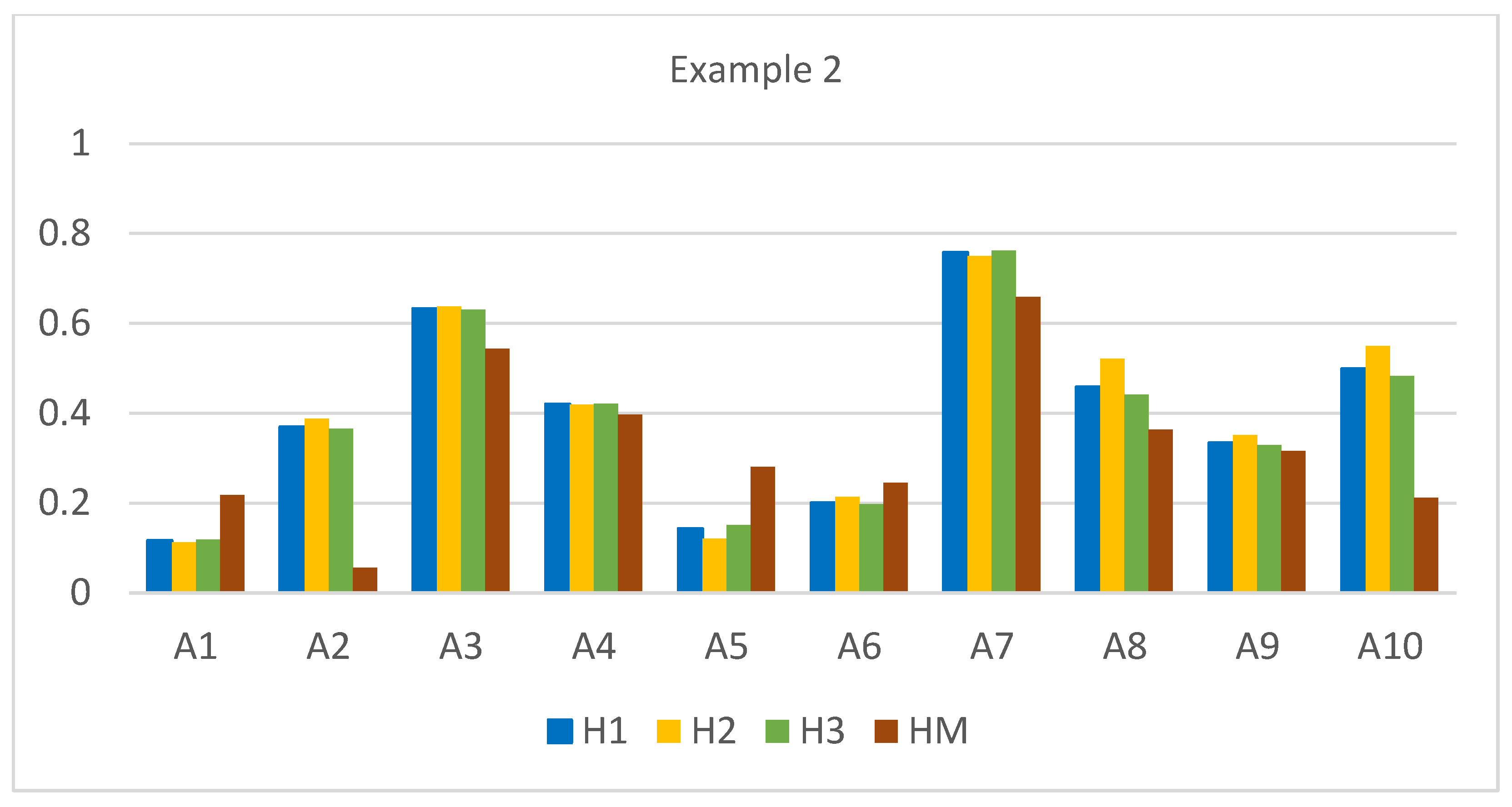
Alternative	dEH1	Value	Range	dEH2	Value	Range	dEH3	Value	Range	dM	Value	Range
		H1	H1		H2	H2		H3	H3		HM	HM
A1	0.255	0.117	10	0.470	0.113	10	0.097	0.119	10	1.959	0.218	8
A2	0.182	0.370	6	0.324	0.388	6	0.070	0.365	6	2.364	0.056	10
A3	0.106	0.632	2	0.192	0.638	2	0.041	0.630	2	1.141	0.544	2
A4	0.168	0.420	5	0.308	0.419	5	0.064	0.421	5	1.510	0.397	3
A5	0.248	0.143	9	0.466	0.121	9	0.093	0.151	9	1.800	0.281	6
A6	0.231	0.201	8	0.417	0.214	8	0.088	0.198	8	1.891	0.245	7
A7	0.070	0.758	1	0.133	0.750	1	0.026	0.762	1	0.855	0.659	1
A8	0.156	0.459	4	0.254	0.521	4	0.062	0.441	4	1.594	0.363	4
A9	0.192	0.334	7	0.344	0.351	7	0.074	0.329	7	1.712	0.316	5
A10	0.145	0.499	3	0.238	0.550	3	0.057	0.483	3	1.972	0.212	9
do	0.289			0.530			0.110			2.504

.

Table 4 indicates that the rankings obtained through the Hellwig procedure and Euclidean distance measure are identical, resulting in S(H1, H2) = S(H1, H3) = S(H2, H3) = 1.000. Also, we observed a very strong correlation between Hi obtained by the Pearson coefficient: P(H1, H2) = 0.993, P(H1, H3) = 0.999, and P(H2, H3) = 0.988.

Distinctions arise when comparing Hellwig’s methods based on Euclidean distance and those based on Mahalanobis distance. Nevertheless, in all cases, the rankings converge for alternatives A3, A7, and A8. Discrepancies for the remaining alternatives range from 1 to 6 positions. The Spearman coefficients between the HM measure reveal moderate relationships among these measures: S(H1, HM) = S(H2, HM) = S(H3, HM) = 0.552. A higher Pearson correlation (moderate or strong) was observed when comparing these measures: P(H1, HM) = 0.709, P(H2, HM) = 0.655, and P(H3, HM) = 0.725. The highest concordance for HM is achieved with H3 (0.725). The graphical representation of Hellwig’s measures is depicted in Figure 2.

Note that Hellwig’s approach, neglecting the interaction between criteria, results in an overestimation of the values for the top-scoring alternatives A3, A7, A8, and A10 while comparing with the HM measure. Conversely, it exhibits an opposite deviation for the low-scoring alternatives A1 and A5.

Example 3. 

(from negligible to very strong correlation between criteria).

Table 5. Data and correlation matrix for Example 3.

Alternative	C1	C2	C3	C4			Correlation Matrix
A1	1	2	2	5			C1	C2	C3	C4
A2	4	6	10	10		C1	1.000	0.501	0.328	0.088
A3	5	23	24	33		C2	0.501	1.000	0.676	0.575
A4	3	1	6	10		C3	0.328	0.676	1.000	0.907
A5	2	10	4	8		C4	0.088	0.575	0.907	1.000
A6	4	7	8	6
A7	10	6	12	15
A8	12	20	8	6
A9	3	6	7	10
A10	6	8	10	6
Ideal	12	23	24	33

Legend: Absolute value of the Pearson coefficient.

[0,0.1)	[0.1,0.2)	[0.2,0.3)	[0.3,0.4)	[0.4,0.5)	[0.5,0.6)	[0.6,0.7)	[0.7,0.8)	[0.8,0.9)	[0.9,1.0)	1
negligible	weak			moderate			strong		very strong

presents the data and correlation matrix for the criteria in Example 3. In this instance, discrepancies in the correlation coefficients range from 0.088 to 0.907. The strongest Pearson correlation is observed between criterion C3 and C4 (0.907), followed by C3 and C2 (0.676), and C4 and C2 (0.575). Meanwhile, the lowest Pearson coefficient is found between C4 and C1 (0.088).

The outcomes of various Hellwig’s measures obtained in Example 3 are presented in

Table 6. The distance values, measure values, and rank-ordering of alternatives obtained by different variants of Hellwig’s measure (Example 3).

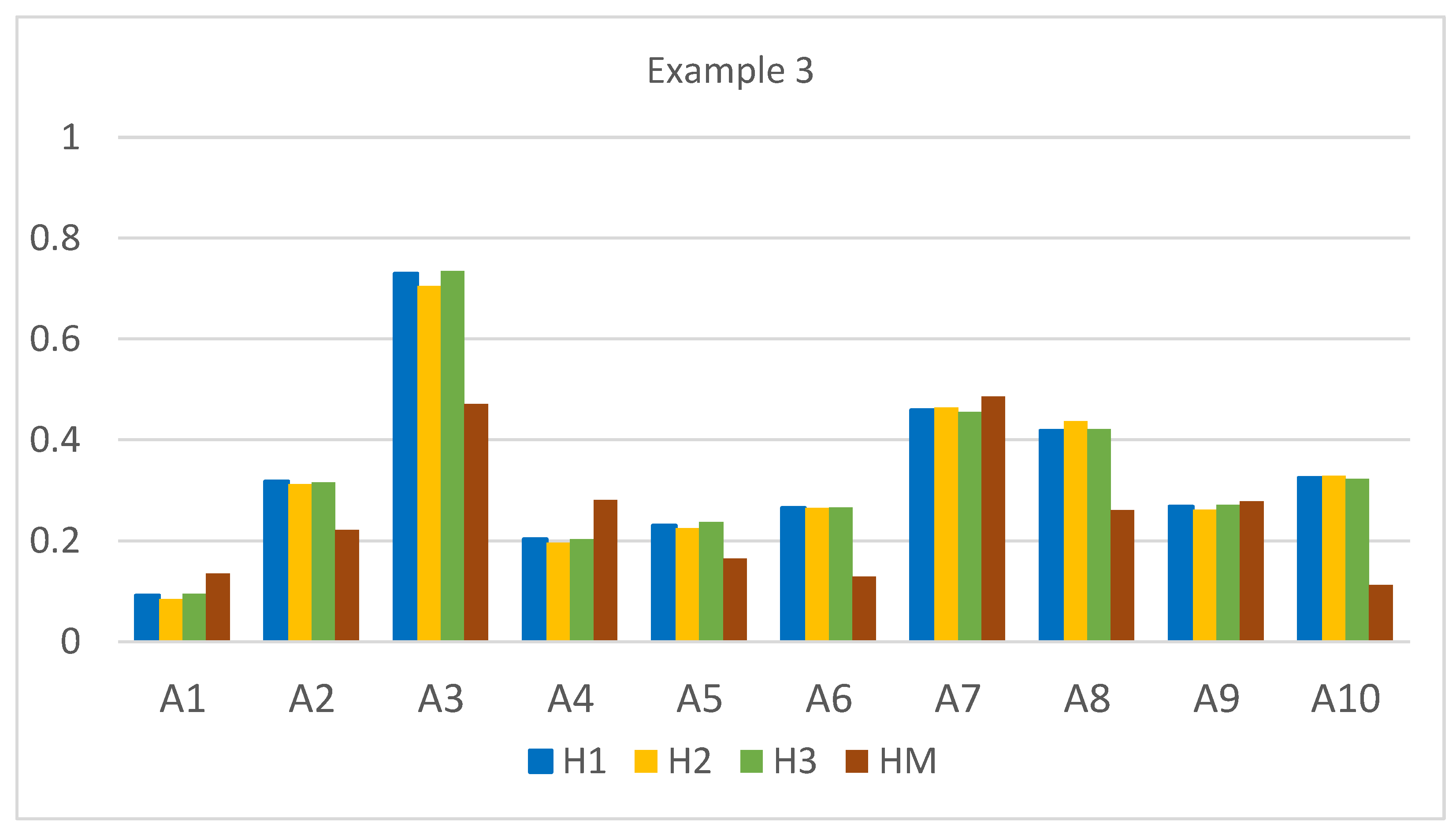
Alternative	dEHI	Value	Range	dEH2	Value	Range	dEH3	Value	Range	dM	Value	Range
		H1	H1		H2	H2		H3	H3		HM	HM
A1	0.310	0.092	10	0.494	0.084	10	0.120	0.095	10	2.223	0.135	8
A2	0.233	0.318	5	0.371	0.312	5	0.090	0.316	5	2.001	0.221	6
A3	0.092	0.730	1	0.159	0.705	1	0.035	0.735	1	1.360	0.471	2
A4	0.272	0.204	9	0.434	0.196	9	0.105	0.203	9	1.848	0.281	3
A5	0.263	0.231	8	0.418	0.225	8	0.101	0.237	8	2.146	0.165	7
A6	0.251	0.266	7	0.397	0.265	6	0.097	0.266	7	2.239	0.129	9
A7	0.185	0.460	2	0.289	0.464	2	0.072	0.455	2	1.320	0.486	1
A8	0.199	0.419	3	0.304	0.437	3	0.076	0.421	3	1.900	0.261	5
A9	0.250	0.269	6	0.398	0.262	7	0.096	0.271	6	1.857	0.278	4
A10	0.231	0.325	4	0.362	0.329	4	0.089	0.323	4	2.282	0.112	10
do	0.342			0.540			0.132			2.570

.

Table 6 indicates that the rankings obtained through the Hellwig procedure and Euclidean distance measure are quite similar, resulting in S(H1, H2) = 0.988, S(H1, H3) = 1, and S(H2, H3) = 0.988. Similarly, the Pearson coefficient shows very strong correlation: P(H1, H2) = 0.998, P(H1, H3) 0.9998, and P(H2, H3) = 0.997.

More distinctions arise when comparing Hellwig’s methods based on Euclidean distance and those based on Mahalanobis distance. In all cases, discrepancies for the alternatives range from 1 to 6 positions. The Spearman coefficients between the HM measure reveal week S(H2, HM) = 0.382 or moderate S(H1, HM) = 0.442 and S(H3, HM) = 0.442 correlation among these measures. A strong Pearson correlation was observed when comparing these measures: P(H1, HM) = 0.755, P(H2, HM) = 0.747, and P(H3, HM) = 0.751. The highest concordance for HM is achieved with H1 (0.755). The graphical representation of Hellwig’s measures is depicted in Figure 3.

Please note that Hellwig’s methods, when utilizing Euclidean distance measurement, lead to an overestimation of values for high-scoring alternatives A3, A8, and A10 while comparing with HM measure. Conversely, it exhibits an opposite deviation for lower-scoring alternatives A1 and A4.

Example 4. 

(strong or very strong correlation between criteria).

Table 7. Data and correlation matrix for Example 4.

Alternative	C1	C2	C3	C4			Correlation Matrix
A1	2	4	3	6			C1	C2	C3	C4
A2	5	10	9	10		C1	1.000	0.730	0.723	0.723
A3	7	8	9	9		C2	0.730	1.000	0.801	0.910
A4	3	6	5	10		C3	0.723	0.801	1.000	0.748
A5	6	10	10	13		C4	0.723	0.910	0.748	1.000
A6	3	6	4	6
A7	6	12	6	14
A8	8	12	10	16
A9	3	6	4	6
A10	6	5	3	7
Ideal	8	12	10	16

Legend: Absolute value of the Pearson coefficient.

[0,0.1)	[0.1,0.2)	[0.2,0.3)	[0.3,0.4)	[0.4,0.5)	[0.5,0.6)	[0.6,0.7)	[0.7,0.8)	[0.8,0.9)	[0.9,1.0)	1
negligible	weak			moderate			strong		very strong

presents both the data and the correlation matrix for the criteria outlined in Example 4. It is noteworthy that we observe high Pearson correlation coefficients ranging from 0.723 (between C3 and C1 or C4 and C1) to 0.910 (between C4 and C2).

The outcomes of various Hellwig’s measures obtained in Example 4 are presented in

Table 8. The distance values, measure values, and rank-ordering of alternatives obtained by different variants of Hellwig’s measure (Example 4).

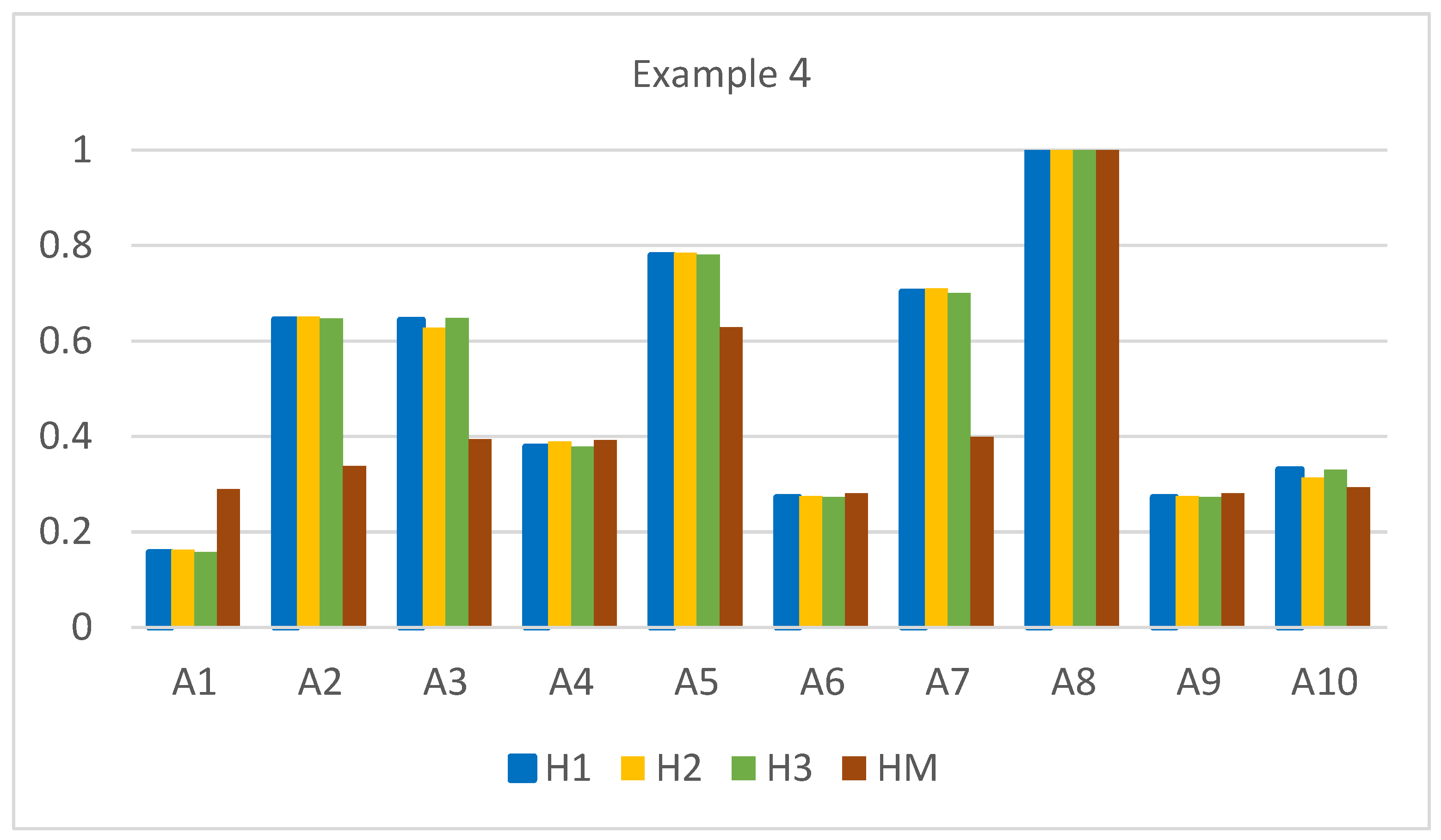
Alternative	dEH1	Value	Range	dEH2	Value	Range	dEH3	Value	Range	dM	Value	Range
		H1	H1		H2	H2		H3	H3		HM	HM
A1	0.162	0.157	10	0.500	0.162	10	0.055	0.157	10	1.552	0.289	8
A2	0.068	0.645	4	0.208	0.651	4	0.023	0.647	5	1.446	0.338	6
A3	0.068	0.644	5	0.222	0.628	5	0.023	0.648	4	1.324	0.394	4
A4	0.119	0.378	6	0.365	0.389	6	0.041	0.378	6	1.326	0.392	5
A5	0.042	0.780	2	0.128	0.785	2	0.014	0.781	2	0.810	0.629	2
A6	0.140	0.273	8	0.432	0.275	8	0.047	0.273	8	1.573	0.280	9
A7	0.057	0.703	3	0.173	0.710	3	0.020	0.700	3	1.312	0.399	3
A8	0.000	1.000	1	0.000	1.000	1	0.000	1.000	1	0.000	1.000	1
A9	0.140	0.273	8	0.432	0.275	8	0.047	0.273	8	1.573	0.28	9
A10	0.129	0.331	7	0.410	0.313	7	0.044	0.33	7	1.544	0.293	7
do	0.192			0.597			0.065			2.183

.

Table 8 highlights discrepancies in rankings for Hellwig’s measures based on Euclidean distance and various normalization formulas, though these differences are marginal. Spearman coefficients between Hellwig’s measures using Euclidean distance are as follows: S(H1, H2) = 1, S(H1, H3) = 0.987, and S(H2, H3) = 0.987. Similarly, a very strong correlation is observed for the Pearson coefficient: P(H1, H2) = 0.999, P(H1, H3) = 0.99998, and P(H2, H3) = 0.999.

For alternatives A5, A7, A8, and A10, rankings consistently converge in all cases. Disparities for the remaining alternatives range only from 1 to 2 positions. Moreover, the Spearman coefficients between the HM measure and other classical Hellwig measures are very strong: S(H1, HM) = 0.921, S(H2, HM) = 0.921, and S(H3, HM) = 0.947. Similarly, a high Pearson correlation is observed when comparing these measures: P(H1, HM) = 0.827, P(H2, HM) = 0.829, and P(H3, HM) = 0.827. The highest concordance for HM is achieved with H2 for the Pearson coefficient and H3 for the Spearman coefficient. The graphical representation of the results for Hellwig’s measures is depicted in Figure 4.

It is worth noting that the alternative in the first position, according to the HM measure, has a value of 1. Additionally, Hellwig’s approach, neglecting the interaction between criteria, results in an overestimation of the values for the high-scoring alternatives A2, A3, A5, and A7 when compared with the HM measure. Conversely, the low-scoring alternative A1 is underestimated according to the HM measure.

Example 5. 

(moderate and strong correlation between criteria).

Table 9. Data and correlation matrix for Example 5.

Alternative	C1	C2	C3	C4			Correlation Matrix
A1	2	4	3	6			C1	C2	C3	C4
A2	5	10	9	10		C1	1.000	0.720	0.656	0.670
A3	7	8	9	9		C2	0.720	1.000	0.711	0.731
A4	3	6	5	10		C3	0.656	0.711	1.000	0.747
A5	6	9	10	13		C4	0.670	0.731	0.747	1.000
A6	4	6	4	5
A7	6	12	6	9
A8	8	12	8	16
A9	3	6	3	6
A10	6	5	3	7
Ideal	8	12	10	16

Legend: Absolute value of the Pearson coefficient.

[0,0.1)	[0.1,0.2)	[0.2,0.3)	[0.3,0.4)	[0.4,0.5)	[0.5,0.6)	[0.6,0.7)	[0.7,0.8)	[0.8,0.9)	[0.9,1.0)	1
negligible	weak			moderate			strong		very strong

presents both the data and the correlation matrix for the criteria outlined in Example 5. The Pearson coefficient varies from 0.656 (between C4 and C1) to 0.747 (between C4 and C3).

The outcomes of various Hellwig’s measures obtained in Example 5 are presented in

Table 10. The distance values, measure values, and rank-ordering of alternatives are obtained by different variants of Hellwig’s measure (Example 5).

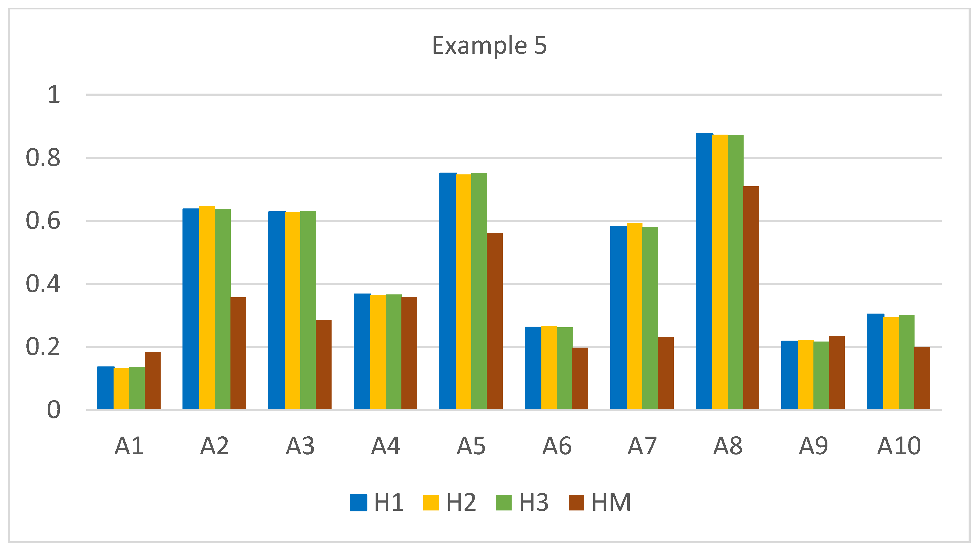
Alternative	dEH1	Value	Range	dEH2	Value	Range	dEH3	Value	Range	dM	Value	Range
		H1	H1		H2	H2		H3	H3		HM	HM
A1	0.166	0.135	10	0.489	0.134	10	0.056	0.136	10	1.657	0.184	10
A2	0.070	0.636	3	0.198	0.648	3	0.024	0.638	3	1.303	0.358	4
A3	0.072	0.628	4	0.210	0.629	4	0.024	0.631	4	1.451	0.285	5
A4	0.122	0.366	6	0.359	0.364	6	0.041	0.366	6	1.301	0.359	3
A5	0.048	0.750	2	0.143	0.747	2	0.016	0.752	2	0.889	0.562	2
A6	0.142	0.261	8	0.414	0.267	8	0.048	0.262	8	1.628	0.198	9
A7	0.081	0.581	5	0.229	0.594	5	0.027	0.580	5	1.560	0.231	7
A8	0.024	0.875	1	0.071	0.873	1	0.008	0.872	1	0.588	0.710	1
A9	0.150	0.217	9	0.439	0.223	9	0.051	0.217	9	1.552	0.235	6
A10	0.134	0.303	7	0.399	0.294	7	0.045	0.302	7	1.623	0.200	8
do	0.192			0.565			0.065			2.030

.

Table 10 highlights discrepancies in rankings for Hellwig’s measures based on Euclidean distance and various normalization formulas. Spearman coefficients between Hellwig’s measures using Euclidean distance are identical: S(H1, H2) = S(H1, H3) = S(H2, H3) = 1, which denotes these same rank ordering alternatives. Also, a very strong correlation is observed for the Pearson coefficient: P(H1, H2) = 0.9996, P(H1, H3) = 0.99997, and P(H2, H3) = 0.9996, though these differences in rating are minimal.

For alternatives A1, A5, and A8, rankings consistently converge in all cases. Disparities for the remaining alternatives range only from 1 to 3 positions. Moreover, the Spearman coefficients between the HM measure and other classical Hellwig measures are very strong: S(H1, HM) = 0.842, S(H2, HM) = 0.842, and S(H3, HM) = 0.842. Similarly, a high Pearson correlation is observed when comparing these measures: P(H1, HM) = 0.821, P(H2, HM) = 0.812, and P(H3, HM) = 0.819. The highest concordance for HM is achieved with H1. The graphical representation of the results for Hellwig’s measures is depicted in Figure 5.

It is worth noting that Hellweg’s methods based on Euclidean distance, neglecting the interaction between criteria, result in an overestimation of the values for the high-scoring alternatives A2, A3, A5, A7, and A8. Conversely, the low-scoring alternatives A1 and A9 are underestimated when compared to the HM measure.

Table 11. Comparison results obtained in the examples.

Example	Correlation between Criteria	Relationships between Hi Measures	Relationships between Hi and HM Measure
Example 1	Negligible or week	Spearman: very strong	Spearman: strong or very strong
		Pearson: very strong	Pearson: very strong
Example 2	From weak to very strong	Spearman: very strong	Spearman: moderate
		Pearson: very strong	Pearson: moderate or strong
Example 3	From negligible to very strong	Spearman: very strong	Spearman: week or moderate
		Pearson: very strong	Pearson: strong
Example 4	Strong and very strong	Spearman: very strong	Spearman: very strong
		Pearson: very strong	Pearson: strong
Example 5	Moderate and strong	Spearman: very strong	Spearman: strong
		Pearson: very strong	Pearson: strong

compares the results obtained in the five examples.

The results can be summarized as follows:

Firstly, it should be noted that the normalization formula when the Euclidean distance is implemented has an impact on the final ranking but is only marginal. However, this does not occur with Mahalanobis distance, as the results remain the same regardless of the type of normalization employed.

Secondly, it can be observed that the rankings obtained using classical Hellwig methods based on Euclidean distance and Hellwig methods based on Mahalanobis distance are different when there is a certain dependence within the data. Those results are consistent with other results in the literature [31]. Even in the case of moderate or small relationships between criteria, the ratings obtained by classical Hellwig’s methods and those of HM do not coincide. It is also difficult to say which of the normalization formulas, in the case of the Euclidean-based Hellwig method, gives results more consistent with Mahalanobis distance-based Hellwig method concerning the Pearson coefficient.

Thirdly, we can observe that Hellwig’s method, neglecting the interaction between criteria, results usually in an overestimation of the values for the high-scoring alternatives. Conversely, the low-scoring alternatives are underestimated when compared with their values in the Mahalanobis distance-based Hellwig’s method. It should be noted that these results are consistent with findings in the literature, where TOPSIS methods based on Euclidean and Mahalanobis distances were compared [31].

5. Conclusions

In the paper, we proposed the Mahalanobis distance-based Hellwig method, incorporating dependencies among criteria. We also investigated the impact of the distance measure (Euclidean and Mahalanobis) and normalization (vector normalization, Min-Max method, Sum method) in the several variants of Hellwig’s procedure. We analyze five illustrative examples that differ in relationships between criteria.

Summing up, the contributions of the article include the following:

• Developing a modification of the Hellwig measure by utilizing the Mahalanobis distance, which considers correlations with different criteria, enables us to effectively account for the asymmetrical relationships between criteria.
• Investigating the impact of the distance measure and normalization variants of Hellwig procedures for the evaluation and rank ordering of alternatives.
• Analyzing the impact of the correlation between criteria on the consistency of results obtained using different variants of Hellwig’s method.

The Mahalanobis distance proves valuable when dealing with asymmetric datasets or datasets featuring correlated variables. Asymmetric datasets often exhibit varying degrees of correlation between variables, and the Mahalanobis distance provides a means to adjust for these correlations. In contrast to the Euclidean distance, which assumes independence among variables, the Mahalanobis distance considers variable relationships by incorporating the covariance matrix.

Consequently, this study shows that the multi-criteria HM method, relying on the Mahalanobis distance, proves effective in addressing correlations between criteria—a critical aspect in the context of asymmetric data. This methodology enables a more accurate reflection of the true data structure, mitigating potential errors associated with assuming criteria independence. At the same time, the Euclidean distance may be less suitable for datasets with asymmetric dependencies between criteria. It neglects information regarding correlation and data structure, potentially resulting in inaccuracies when criteria exhibit strong correlation or asymmetric dependencies.

This work acknowledges certain limitations that will serve as subjects for further research. In the paper, the focus was limited to a few examples that served as illustrations of the challenges and consequences associated with the choice of a variant of Hellwig’s method. Further research could delve into considering different normalization techniques to better understand and potentially mitigate their impact on rankings, especially when utilizing Euclidean distance. Future studies may aim to explore and quantify the extent of criteria interdependence, seeking to establish patterns or criteria characteristics that contribute to the divergence in rankings between Hellwig methods based on Euclidean distance and those based on Mahalanobis distance. Future investigations could focus on the interaction effects between criteria, examining the nuances that lead to the overestimation of high-scoring alternatives and the underestimation of low-scoring ones, particularly in the context of variants of Hellwig’s method. It would be beneficial to extend the study to different datasets to assess the generalizability of the observed patterns and to identify any dataset-specific factors that may influence the results. Consideration of comparisons with alternative methods beyond the TOPSIS approach could provide a broader perspective on the performance of Hellwig’s methods and their variations. By addressing these aspects in future research, a more comprehensive understanding of the observed phenomena and potential strategies for improvement or mitigation can be achieved.

References

- Figueira; Ehrgott, M.; Greco, S. Multiple Criteria Decision Analysis: State of the Art Surveys; Springer Science + Business Media: Berlin/Heidelberg, Germany, 2005. [Google Scholar]
- Roy, B. Multicriteria Methodology for Decision Aiding; Kluwer Academic Publisher: Dordrecht, The Netherlands, 1996. [Google Scholar]
- Basílio, M.P.; Pereira, V.; Costa, H.G.; Santos, M.; Ghosh, A. A Systematic Review of the Applications of Multi-Criteria Decision Aid Methods (1977–2022). Electronics 2022, 11, 1720. [Google Scholar] [CrossRef]
- Yalcin, A.S.; Kilic, H.S.; Delen, D. The Use of Multi-Criteria Decision-Making Methods in Business Analytics: A Comprehensive Literature Review. Technol. Forecast. Soc. Change 2022, 174, 121193. [Google Scholar] [CrossRef]
- Štilić, A.; Puška, A. Integrating Multi-Criteria Decision-Making Methods with Sustainable Engineering: A Comprehensive Review of Current Practices. Eng 2023, 4, 1536–1549. [Google Scholar] [CrossRef]
- Cegan, J.C.; Filion, A.M.; Keisler, J.M.; Linkov, I. Trends and Applications of Multi-Criteria Decision Analysis in Environmental Sciences: Literature Review. Environ. Syst. Decis. 2017, 37, 123–133. [Google Scholar] [CrossRef]
- Diaz-Balteiro, L.; González-Pachón, J.; Romero, C. Measuring Systems Sustainability with Multi-Criteria Methods: A Critical Review. Eur. J. Oper. Res. 2017, 258, 607–616. [Google Scholar] [CrossRef]
- Kaya, İ.; Çolak, M.; Terzi, F. A Comprehensive Review of Fuzzy Multi Criteria Decision Making Methodologies for Energy Policy Making. Energy Strategy Rev. 2019, 24, 207–228. [Google Scholar] [CrossRef]
- Hwang, C.-L.; Yoon, K. (Eds.) Methods for Multiple Attribute Decision Making; Lecture Notes in Economics and Mathematical Systems; Springer: Berlin/Heidelberg, Germany, 1981; ISBN 978-3-642-48318-9. [Google Scholar]
- Hellwig, Z. Zastosowanie Metody Taksonomicznej Do Typologicznego Podziału Krajów Ze Względu Na Poziom Ich Rozwoju Oraz Zasoby i Strukturę Wykwalifikowanych Kadr [Application of the Taxonomic Method to the Typological Division of Countries According to the Level of Their Development and the Resources and Structure of Qualified Personnel]. Przegląd Statystyczny 1968, 4, 307–326. [Google Scholar]
- Opricovic, S.; Tzeng, G.-H. Compromise Solution by MCDM Methods: A Comparative Analysis of VIKOR and TOPSIS. Eur. J. Oper. Res. 2004, 156, 445–455. [Google Scholar] [CrossRef]
- Roszkowska, E.; Filipowicz-Chomko, M.; Wachowicz, T. Using Individual and Common Reference Points to Measure the Performance of Alternatives in Multiple Criteria Evaluation. Oper. Res. Decis. 2020, 30, 77–96. [Google Scholar] [CrossRef]
- Rezaei, J. Best-Worst Multi-Criteria Decision-Making Method. Omega 2015, 53, 49–57. [Google Scholar] [CrossRef]
- Konarzewska-Gubała, E. Bipolar: Multiple Criteria Decision Aid Using Bipolar Refernce System. LAMSADE Cashier Doc. 1989, 56. [Google Scholar]
- Jahan, A.; Edwards, K.L. A State-of-the-Art Survey on the Influence of Normalization Techniques in Ranking: Improving the Materials Selection Process in Engineering Design. Mater. Des. 2014, 65, 335–342. [Google Scholar] [CrossRef]
- Çelen, A. Comparative Analysis of Normalization Procedures in TOPSIS Method: With an Application to Turkish Deposit Banking Market. Informatica 2014, 25, 185–208. [Google Scholar] [CrossRef]
- Chakraborty, S.; Yeh, C.-H. A Simulation Based Comparative Study of Normalization Procedures in Multiattribute Decision Making. In Proceedings of the 6th Conference on 6th WSEAS International Conference on Artificial Intelligence, Knowledge Engineering and Data Bases, Corfu Island, Greece, 16–19 February 2007; Citeseer: State College, PA, USA, 2007; Volume 6, pp. 102–109. [Google Scholar]
- Chakraborty, S.; Yeh, C.-H. A Simulation Comparison of Normalization Procedures for TOPSIS. In Proceedings of the 2009 International Conference on Computers and Industrial Engineering (CIE39), Troyes, France, 6–9 July 2009; IEEE, Institute of Electrical and Electronics Engineers: Piscataway, NJ, USA, 2009; pp. 1815–1820. [Google Scholar]
- Milani, A.S.; Shanian, A.; Madoliat, R.; Nemes, J.A. The Effect of Normalization Norms in Multiple Attribute Decision Making Models: A Case Study in Gear Material Selection. Struct. Multidiscip. Optim. 2005, 29, 312–318. [Google Scholar] [CrossRef]
- Palczewski, K.; Sałabun, W. Influence of Various Normalization Methods in PROMETHEE II: An Empirical Study on the Selection of the Airport Location. Procedia Comput. Sci. 2019, 159, 2051–2060. [Google Scholar] [CrossRef]
- Pavličić, D. Normalization Affects the Results of MADM Methods. Yugosl. J. Oper. Res. 2001, 11, 251–265. [Google Scholar]
- Vafaei, N.; Ribeiro, R.A.; Camarinha-Matos, L.M. Normalization Techniques for Multi-Criteria Decision Making: Analytical Hierarchy Process Case Study. In Technological Innovation for Cyber-Physical Systems, Proceedings of the 7th IFIP 5.5/SOCOLNET Doctoral Conference on Computing, Electrical and Industrial Systems, DoCEIS 2016, Costa de Caparica, Portugal, 11–13 April 2016; Camarinha-Matos, L.M., Falcão, A.J., Vafaei, N., Najdi, S., Eds.; Springer International Publishing: Cham, Switzerland, 2016; pp. 261–269. [Google Scholar]
- Zavadskas, E.K.; Zakarevicius, A.; Antucheviciene, J. Evaluation of Ranking Accuracy in Multi-Criteria Decisions. Informatica 2006, 17, 601–618. [Google Scholar] [CrossRef]
- Mahalanobis, P.C. On the Generalised Distance in Statistics. Proc. Natl. Inst. Sci. 1936, 2, 49–55. [Google Scholar]
- Ghojogh, B.; Ghodsi, A.; Karray, F.; Crowley, M. Spectral, Probabilistic, and Deep Metric Learning: Tutorial and Survey. arXiv 2022, arXiv:2201.09267. [Google Scholar]
- Liu, D.; Qi, X.; Qiang, F.; Li, M.; Zhu, W.; Zhang, L.; Abrar Faiz, M.; Khan, M.I.; Li, T.; Cui, S. A Resilience Evaluation Method for a Combined Regional Agricultural Water and Soil Resource System Based on Weighted Mahalanobis Distance and a Gray-TOPSIS Model. J. Clean. Prod. 2019, 229, 667–679. [Google Scholar] [CrossRef]
- Ponce, R.V.; Alcaraz, J.L.G. Evaluation of Technology Using TOPSIS in Presence of Multi-Collinearity in Attributes: Why Use the Mahalanobis Distance? Rev. Fac. Ing. Univ. Antioq. 2013, 31–42. [Google Scholar] [CrossRef]
- Antuchevičienė, J.; Zavadskas, E.K.; Zakarevičius, A. Multiple Criteria Construction Management Decisions Considering Relations between Criteria. Technol. Econ. Dev. Econ. 2010, 16, 109–125. [Google Scholar] [CrossRef]
- Wang, Z.-X.; Li, D.-D.; Zheng, H.-H. The External Performance Appraisal of China Energy Regulation: An Empirical Study Using a TOPSIS Method Based on Entropy Weight and Mahalanobis Distance. Int. J. Environ. Res. Public Health 2018, 15, 236. [Google Scholar] [CrossRef] [PubMed]
- Chang, C.-H.; Lin, J.-J.; Lin, J.-H.; Chiang, M.-C. Domestic Open-End Equity Mutual Fund Performance Evaluation Using Extended TOPSIS Method with Different Distance Approaches. Expert Syst. Appl. 2010, 37, 4642–4649. [Google Scholar] [CrossRef]
- Wang, Z.-X.; Wang, Y.-Y. Evaluation of the Provincial Competitiveness of the Chinese High-Tech Industry Using an Improved TOPSIS Method. Expert Syst. Appl. 2014, 41, 2824–2831. [Google Scholar] [CrossRef]
- Ozmen, M. Logistics Competitiveness of OECD Countries Using an Improved TODIM Method. Sādhanā 2019, 44, 108. [Google Scholar] [CrossRef]
- Wasid, M.; Ali, R. Multi-Criteria Clustering-Based Recommendation Using Mahalanobis Distance. Int. J. Reason. -Based Intell. Syst. 2020, 12, 96. [Google Scholar] [CrossRef]
- Dong, H.; Yang, K.; Bai, G. Evaluation of TPGU Using Entropy—Improved TOPSIS—GRA Method in China. PLoS ONE 2022, 17, e0260974. [Google Scholar] [CrossRef]
- Xiang, S.; Nie, F.; Zhang, C. Learning a Mahalanobis Distance Metric for Data Clustering and Classification. Pattern Recognit. 2008, 41, 3600–3612. [Google Scholar] [CrossRef]
- Ghosh-Dastidar, S.; Adeli, H. Wavelet-Clustering-Neural Network Model for Freeway Incident Detection. Comput. Aided Civ. Infrastruct. Eng. 2003, 18, 325–338. [Google Scholar] [CrossRef]
- Jefmański, B. Intuitionistic Fuzzy Synthetic Measure for Ordinal Data. In Clasification and Data Analysis, Proceedings of the Conference of the Section on Classification and Data Analysis of the Polish Statistical Association, Szczecin, Poland, 18–20 September 2019; Springer: Berlin/Heidelberg, Germany, 2019; pp. 53–72. [Google Scholar]
- Jefmański, B.; Roszkowska, E.; Kusterka-Jefmańska, M. Intuitionistic Fuzzy Synthetic Measure on the Basis of Survey Responses and Aggregated Ordinal Data. Entropy 2021, 23, 1636. [Google Scholar] [CrossRef] [PubMed]
- Kusterka-Jefmańska, M.; Jefmański, B.; Roszkowska, E. Application of the Intuitionistic Fuzzy Synthetic Measure in the Subjective Quality of Life Measurement Based on Survey Data. In Modern Classification and Data Analysis, Proceedings of the Conference of the Section on Classification and Data Analysis of the Polish Statistical Association, Poznań, Poland, 8–10 September 2021; Springer: Berlin/Heidelberg, Germany, 2022; pp. 243–261. [Google Scholar]
- Roszkowska, E. The Intuitionistic Fuzzy Framework for Evaluation and Rank Ordering the Negotiation Offers. In Intelligent and Fuzzy Techniques for Emerging Conditions and Digital Transformation, Proceedings of the International Conference on Intelligent and Fuzzy Systems INFUS 2021, Istanbul, Turkey, 24–26 August 2021; Lecture Notes in Networks and Systems; Kahraman, C., Cebi, S., Onar, S., Oztaysi, B., Tolga, A.C., Sari, I.U., Eds.; Springer: Cham, Switzerland, 2021; Volume 308, pp. 58–65. [Google Scholar]
- Roszkowska, E.; Jefmański, B. Interval-Valued Intuitionistic Fuzzy Synthetic Measure (I-VIFSM) Based on Hellwig’s Approach in the Analysis of Survey Data. Mathematics 2021, 9, 201. [Google Scholar] [CrossRef]
- Roszkowska, E.; Wachowicz, T.; Filipowicz-Chomko, M.; Łyczkowska-Hanćkowiak, A. The Extended Linguistic Hellwig’s Methods Based on Oriented Fuzzy Numbers and Their Application to the Evaluation of Negotiation Offers. Entropy 2022, 24, 1617. [Google Scholar] [CrossRef] [PubMed]
- Mazur-Wierzbicka, E. Towards Circular Economy—A Comparative Analysis of the Countries of the European Union. Resources 2021, 10, 49. [Google Scholar] [CrossRef]
- Balcerzak, A.P. Multiple-Criteria Evaluation of Quality of Human Capital in the European Union Countries. Econ. Sociol. 2016, 9, 11–26. [Google Scholar] [CrossRef]
- Łuczak, A.; Wysocki, F. Rozmyta Wielokryterialna Metoda Hellwiga Porządkowania Liniowego Obiektów [Fuzzy Multi-Criteria Hellwig’s Method of Linear Ordering of Objects]. Pr. Nauk. Akad. Ekon. We Wrocławiu Taksonomia 2007, 14, 330–340. [Google Scholar]
- Golejewska, A. A Comparative Analysis of the Socio-Economic Potential of Polish Regions. Stud. Ind. Geogr. Comm. Pol. Geogr. Soc. 2016, 30, 7–22. [Google Scholar] [CrossRef]
- Barska, A.; Jędrzejczak-Gas, J.; Wyrwa, J. Poland on the Path towards Sustainable Development—A Multidimensional Comparative Analysis of the Socio-Economic Development of Polish Regions. Sustainability 2022, 14, 10319. [Google Scholar] [CrossRef]
- Jędrzejczak-Gas, J.; Barska, A. Assessment of the Economic Development of Polish Regions in the Context of the Implementation of the Concept of Sustainable Development—Taxonomic Analysis. Eur. J. Sustain. Dev. 2019, 8, 222. [Google Scholar] [CrossRef]
- Iwacewicz-Orłowska, A.; Sokołowska, D. Ranking of EU Countries in Terms of the Value of Environmental Governance Indicators in 2010 and 2015. Ekon. Sr. Econ. Environ. 2018, 66, 13. [Google Scholar]
- Sompolska-Rzechuła, A. Selection of the Optimal Way of Linear Ordering of Objects: Case of Sustainable Development in EU Countries. Stat. Stat. Econ. J. 2021, 101, 24–36. [Google Scholar]
- Reiff, M.; Surmanová, K.; Balcerzak, A.P.; Pietrzak, M.B. Multiple Criteria Analysis of European Union Agriculture. J. Int. Stud. 2016, 9, 62–74. [Google Scholar] [CrossRef]
- Gostkowski, M.; Koszela, G. Application of the Linear Ordering Methods to Analysis of the Agricultural Market in Poland. Metod. Ilościowe W Badaniach Ekon. 2019, 20, 167–177. [Google Scholar] [CrossRef]
- Wysocki, F. Metody Taksonomiczne w Rozpoznawaniu Typów Ekonomicznych Rolnictwa i Obszarów Wiejskich [Taxonomic Methods in Recognizing Economic Types of Agriculture and Rural Areas]; Wydawnictwo Uniwersytetu Przyrodniczego w Poznaniu: Poznan, Poland, 2010; 399p. [Google Scholar]
- Krukowski, A.; Nowak, A.; Różańska-Boczula, M. Evaluation of Agriculture Development in the Member States of the European Union in the Years 2007–2015. In Proceedings of the 31st International Business Information Management Association Conference, Milan, Italy, 25–26 August 2018. [Google Scholar]
- Di Domizio, M. The Competitive Balance in the Italian Football League: A Taxonomic Approach; Department of Communication, University of Teramo: Teramo, Italy, 2008. [Google Scholar]
- Elżbieta Roszko-Wójtowicz, E.; Grzelak, M.M. The Use of Selected Methods of Linear Ordering to Assess the Innovation Performance of the European Union Member States. Econ. Environ. Stud. 2019, 19, 9–30. [Google Scholar]
- Gałecka, M.; Smolny, K. Evaluation of Theater Activity Using Hellwig’s Method. Optim. Econ. Stud. 2018, 38–50. [Google Scholar] [CrossRef]
- Dmytrów, K. Comparison of Several Linear Ordering Methods for Selection of Locations in Order-Picking by Means of the Simulation Methods. Acta Univ. Lodz. Folia Oecon. 2018, 5, 81–96. [Google Scholar] [CrossRef]
- Ahn, B.S.; Park, K.S. Comparing Methods for Multiattribute Decision Making with Ordinal Weights. Comput. Oper. Res. 2008, 35, 1660–1670. [Google Scholar] [CrossRef]
- Ayan, B.; Abacıoğlu, S.; Basilio, M.P. A Comprehensive Review of the Novel Weighting Methods for Multi-Criteria Decision-Making. Information 2023, 14, 285. [Google Scholar] [CrossRef]
- Choo, E.U.; Schoner, B.; Wedley, W.C. Interpretation of Criteria Weights in Multicriteria Decision Making. Comput. Ind. Eng. 1999, 37, 527–541. [Google Scholar] [CrossRef]
- Da Silva, F.F.; Souza, C.L.M.; Silva, F.F.; Costa, H.G.; da Hora, H.R.M.; Erthal, M., Jr. Elicitation of Criteria Weights for Multicriteria Models: Bibliometrics, Typologies, Characteristics and Applications. Braz. J. Oper. Prod. Manag. 2021, 18, 1–28. [Google Scholar] [CrossRef]
- Roszkowska, E. Rank Ordering Criteria Weighting Methods—A Comparative Overview. Optim. Econ. Stud. 2013, 5, 14–33. [Google Scholar] [CrossRef]
- Zardari, N.H.; Ahmed, K.; Shirazi, S.M.; Yusop, Z.B. Weighting Methods and Their Effects on Multi-Criteria Decision Making Model Outcomes in Water Resources Management; Springer: Berlin/Heidelberg, Germany, 2015. [Google Scholar]
- Tzeng, G.-H.; Chen, T.-Y.; Wang, J.-C. A Weight-Assessing Method with Habitual Domains. Eur. J. Oper. Res. 1998, 110, 342–367. [Google Scholar] [CrossRef]