A Discrete-Time Current Control Method for the High-Speed Permanent Magnet Motor Drive Using the Modular Multilevel Converter

Abstract

High-speed permanent magnet motors (HSPMMs) have received attention in direct drive systems from the industry. Modular multilevel converters (MMCs) have become the most practical solution for HSPMMs in industrial applications due to the advantages of their highly modular structure, high-quality output and high reliability. In this article, the symmetrical discrete-time model of the MMC for the HSPMM drive is presented. Based on this symmetrical discrete-time model, the discrete-time current regulator has been designed. Moreover, the submodel (SM) capacitor energy balance models for MMC have been described, and the energy balance control scheme is introduced. Finally, the simulation and experimental results show that the presented discrete-time current regulator has a strong dynamic response at high speed (15 kr/min), and the SM capacitor voltage balance control is also achieved. Compared with the conventional PI current controller, the proposed discrete-time current regulator improves the current loop dynamic performance at high-speed, and the energy balance control scheme can ensure the SM capacitor voltage balance of the MMC.

1. Introduction

With the development of permanent magnet direct drive systems, high-speed permanent magnet motors (HSPMMs) have attracted widespread attention from the industry due to their features such as small size, high power density and free-gearbox operation [1]. HSPMMs are typically used in industrial direct-drive applications, including high-speed blowers, high-speed pumps, flywheel energy storage, and gas generators, etc. [2].

However, HSPMMs are generally driven by three-phase symmetrical full-bridge two-level voltage source inverters (VSIs) which have obvious disadvantages, such as the pulse width modulation (PWM), which causes serious current pulsation. The winding inductance of the HSPMM is generally small, and pulse voltage output from the inverter causes serious current pulsation on the winding. The pulsating current generates additional eddy current losses in the rotor sheath and permanent magnets. Since it is difficult to dissipate heat from the rotor, the additional loss will cause the temperature of the permanent magnets to rise, resulting in the risk of demagnetization [3,4]. Moreover, VSI has high dV/dt, due to the switching of the IGBTs which is not ideal, combined with the stray parameters of the wires and motor windings, the voltage applied to the motor windings has high voltage spikes. Such voltage peaks can easily cause partial discharge and insulation aging of the motor windings, which can lead to serious turn-to-turn short circuits, causing damage to the motor and preventing it from working properly [5,6].

To solve these disadvantages, researches have conducted numerous studies. For instance, the wide bandgap (WBG) devices can reduce the switching losses and increase the switching frequency by tens of times to over 100 kHz, such as SiC and GaN [7,8,9]. But the extremely high switching frequency of WBG devices can cause more severe dV/dt; in addition, the cost of using the WBG devices is still very high and not conducive to use in industrial applications [10].

Another method is to use a sinusoidal filter, such as $LC$ or $LCL$ filter [11,12,13]. The sinusoidal filter can filter out the high-frequency component of the PWM voltage pulses so that the terminal voltage of the motor is sinusoidal, thus eliminating current pulsations and higher dV/dt in the windings [14]. However, the output sinusoidal filter increases the order of the mathematical model of the motor drive system, which makes the control of the motor complicated. Moreover, the sinusoidal filters used in the industrial high-power applications were not considered.

Eventually, multilevel converters have become a more suitable choice for high-power HSPMMs in industrial applications [15], particularly, the modular multilevel converter (MMC) [16]. Compared with other multilevel converters, the MMC presents several features. Firstly, it has a highly modular structure, eliminating the need for multiple isolated DC power supplies and transformers. Secondly, it realizes the high-voltage and high switching frequency multilevel outputs with low-voltage switching devices, which reducing the switching losses. Finally, it also has a common DC bus, which is highly reliable and covers a wide range of power levels [17,18,19].

Presently, many researchers are making considerable efforts to work on the control methods and performance of the MMC. Most of the work is focused on the submodule (SM) capacitor voltage balance of the MMC [17,18,20,21,22,23,24,25,26,27,28]. Li et al. [20] and Dekka et al. [21] proposed an improved MMC topology and submodule topology, respectively, which improves the sub-module capacitance-voltage balancing performance, but increases the complexity of the system and reduces the reliability. Kolluri et al. [22] introduced a frequency adaptive control method based on two-space repetitive control to suppress the second harmonic in the SM capacitor voltage, but does not take into account the starting conditions of the motor. Samajdar and Bhattacharya [23] described a generalized sub-module capacitor energy modification control method, which avoids quantities look-up table calculations during operation. A back-to-back MMC used for motor drives can operate at full speed range, but the back-to-back MMC needs a large number of components, which is several times that of the conventional MMC for motor drive systems [24]. Picas et al. [17] presented the discontinuous modulation technique to reduce the capacitor voltage ripples for the MMC in the motor drive application. Zhao et al. [25] discussed a new coordinated strategy to reduce the average SM capacitor voltage in low-frequency occasions. The SM capacitor voltage ripple estimation and optimal sizing for MMC was studied in [18], which is suitable for variable-speed drive. Nevertheless, from [18,19,20,21,22,23,24], the operation frequencies are all below 100 Hz; these prior works are suitable for low frequency conditions, and do not take into account high-speed operating conditions with a speed above 10 kr/min. Pan et al. [26] developed a SiC-based MMC prototype for high-speed drive, and then, Pan et al. [27] presented a new integrated control method for the high-speed MMC drive, where the motor speed reached 15 kr/min. But Pan et al. [26] and Pan et al. [27] used nearest level modulation (NLM), which is not designed for carrier phase shifting (CPS) modulation. Xia et al. [28] proposed a novel energy balance control method for the motor drive in low-speed and high-speed occasions, respectively. The method is based on the circulating current injection in low-speed region, and the motor speed also reached up to 15 kr/min. But [27,28] adopted the traditional PI current regulator, and did not take into account the degradation of the current loop at high speeds.

To overcome the mentioned disadvantages, the discrete-time current control method for the MMC in the HSPMM drive application is proposed, which replaces the traditional discrete PI current controller and solves the degradation of current loop dynamic control performance at high frequency. At the same time, the energy balance of the capacitor is considered. The main contributions of this study are listed as follows.

(1)

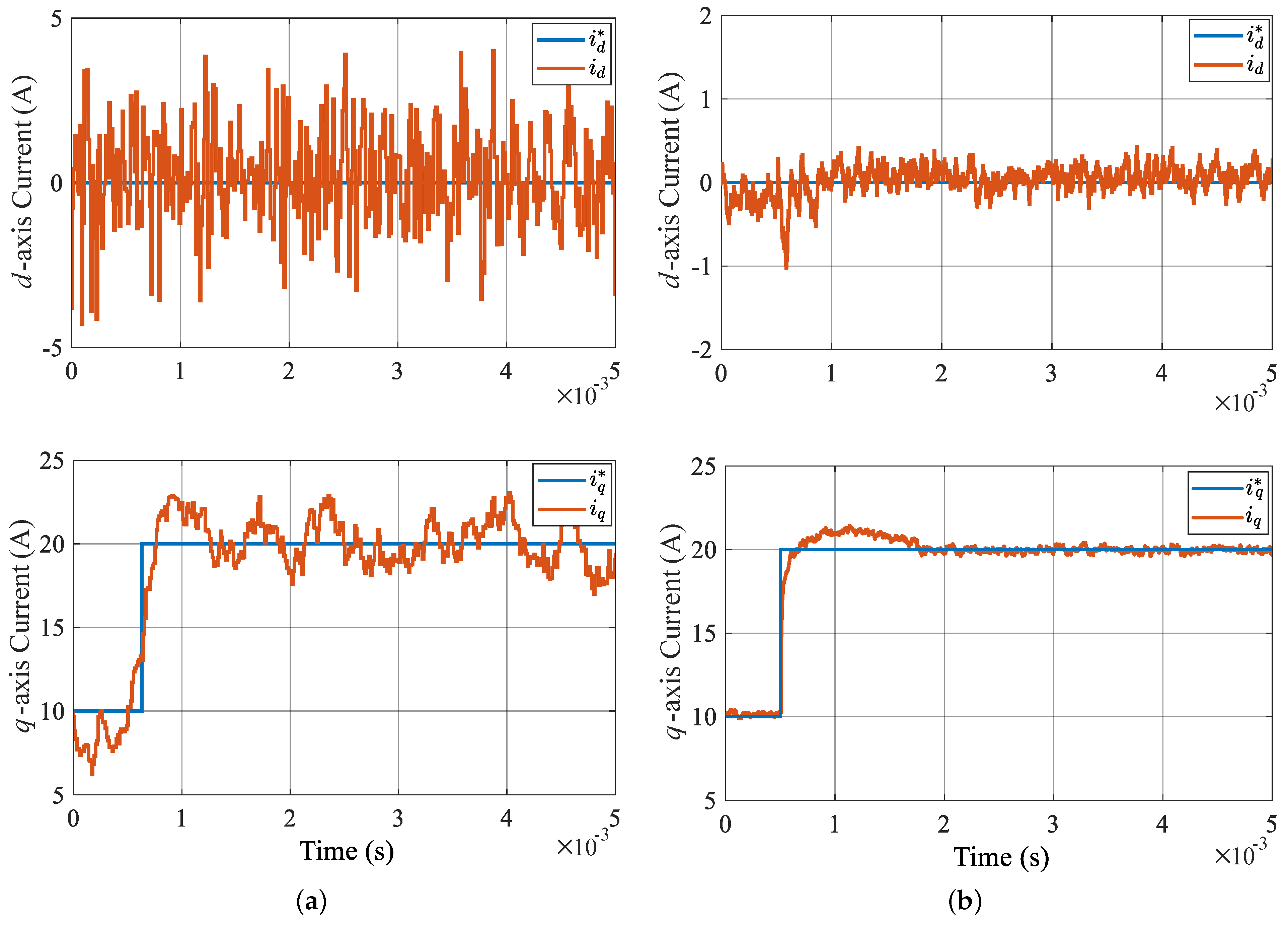
The symmetrical discrete-time model of the MMC for a HSPMM drive is established. Compared with the traditional discrete PI current controller, the proposed discrete-time current regulator can achieve significant dynamic performance at high speed regions.

(2)

The energy balance model for MMC is illustrated, the design of energy balance controller is introduced.

(3)

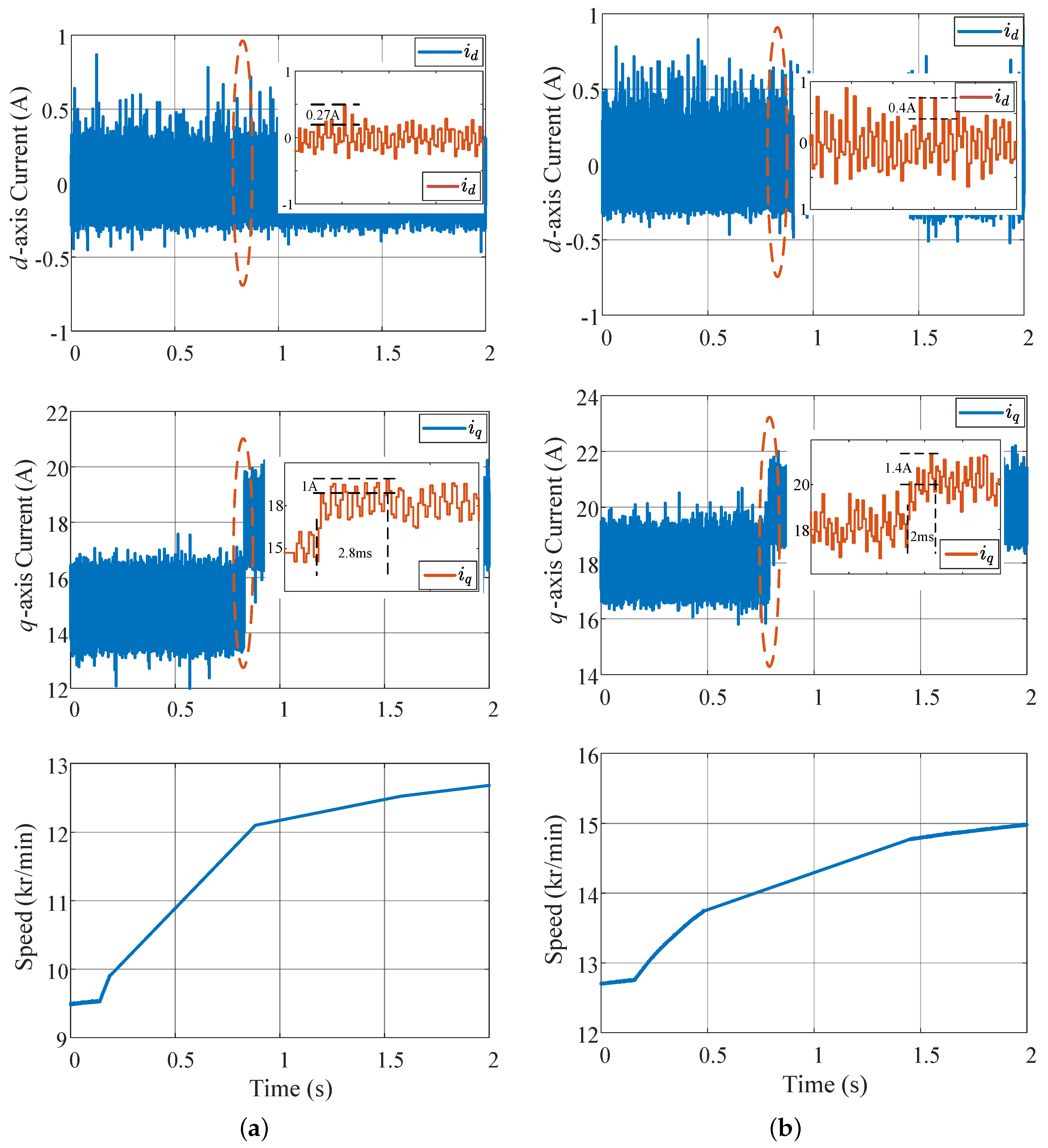
The proposed methods are realized and verified during the dynamic and steady states, and the motor speed reached up to 15 kr/min.

The rest of this article is organized as follows. The MMC topology and circuit architecture are introduced in Section 2. Section 3 describes the discrete-time model of MMC, and proposes the discrete-time current control method. Section 4 presents the energy balance model and controller design of the MMC. Simulation results are shown in Section 5, and experimental results are shown in Section 6. Finally, Section 7 draws the conclusions.

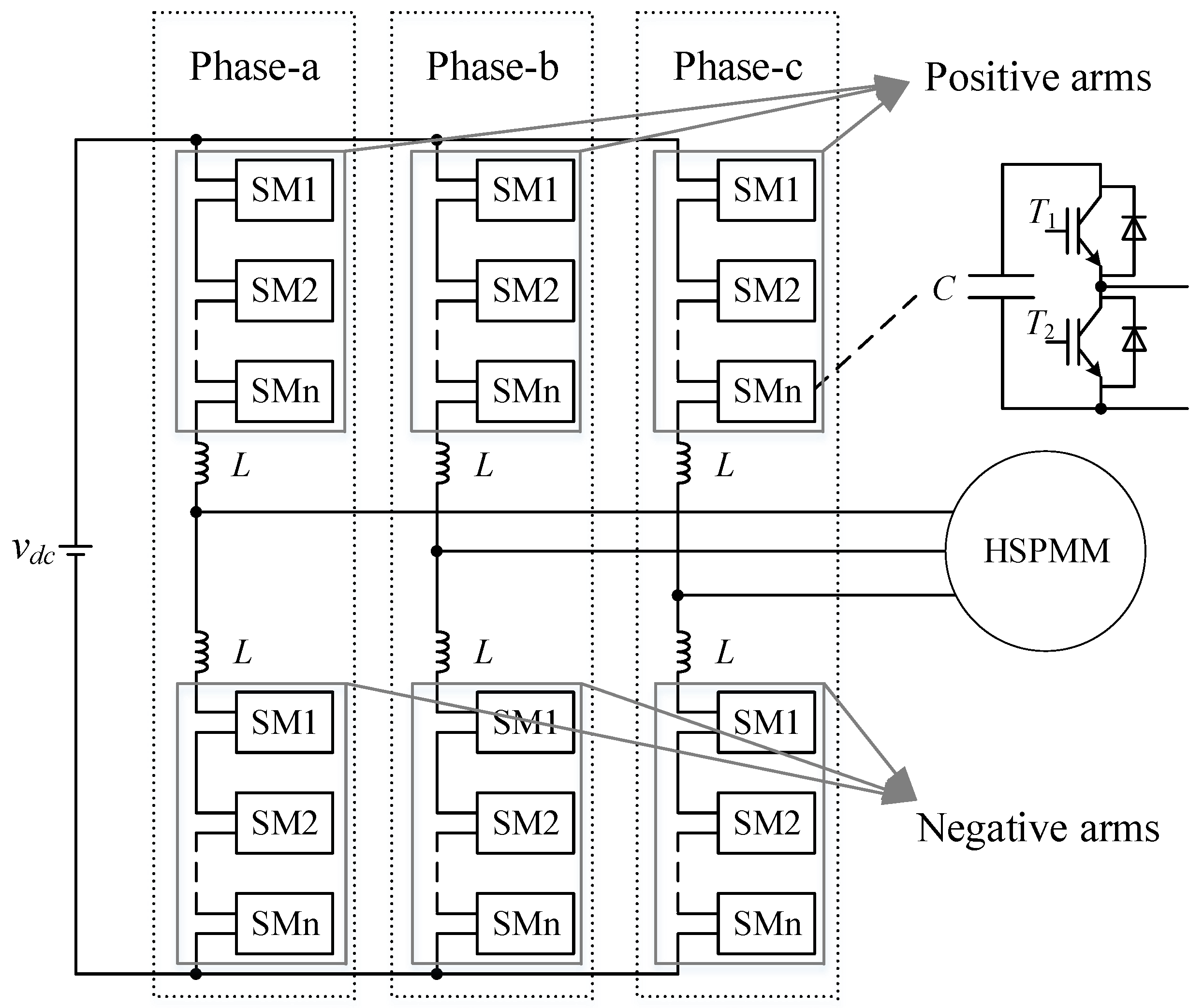
2. MMC Topology and Circuit Architecture

Firstly, the MMC topology is introduced in this section. Then, the circuit architecture is presented.

2.1. MMC Topology Structure

The symmetrical topology structure of the MMC for the high-speed permanent magnet motor is depicted in Figure 1. The MMC consists of symmetrical positive and negative bridge arms; each positive and negative bridge arm contains n identical SM and a series connected bridge arm inductor L. Each SM has a half-bridge structure including a floating DC capacitor C and two fully controlled power devices with anti-parallel diodes. The symmetrical bridge arm inductor L acts as a filter to reduce the high frequency component of the bridge arm current and as a current limiter for the short-circuit current.

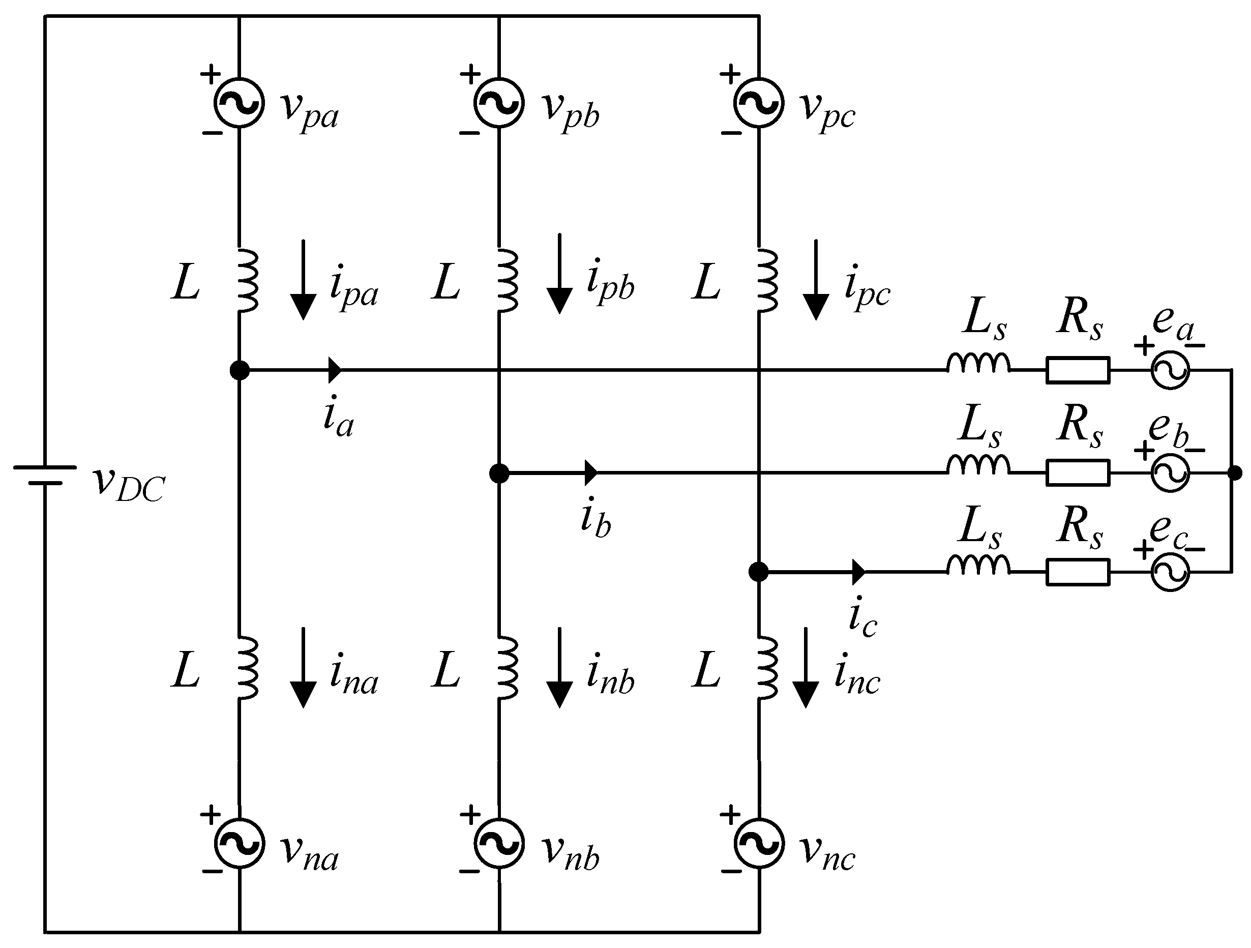
2.2. Circuit Structure

The three-phase symmetrical equivalent circuit of the MMC for the HSPMM drive application is demonstrated in Figure 2. $v_{dc}$ is defined as the DC bus voltage$,v_{pj}$ ($j=a,b,c$) is the positive bridge arm voltage, $v_{nj}$ ($j=a,b,c$) is the negative bridge arm voltage. $i_{pj}$ is the positive bridge arm current, and $i_{nj}$ ($j=a,b,c$) is negative bridge arm current. L is the bridge arm inductance. $i_j$ ($j=a,b,c$) are the three-phase AC output currents. $L_s$ and $R_s$ are the motor stator inductance and resistance, respectively. The back EMFs of the motor are $e_j$ ($j=a,b,c$).

According to Kirchhoff’s law, the voltage follows that:

$$\left\{\begin{array}{cc}\hfill v_{dc}& =v_{pj}+v_{nj}+L\frac{d(i_{pj}+i_{nj})}{dt}\hfill \\ \hfill v_j& =\frac{v_{dc}}{2}-\left(\frac{v_{pj}-v_{nj}}{2}\right)-\frac{L}{2}\frac{d(i_{pj}-i_{nj})}{dt}\hfill \\ \hfill v_j& =R_s{i}_j+L_s\frac{d{i}_j}{dt}+e_j\hfill \end{array}\right.$$

(1)

where $v_j$ is defined as the bridge arm output voltage:

$$\begin{array}{cc}\hfill v_j& =\frac{1}{2}(v_{nj}-v_{pj})\hfill \end{array}$$

(2)

Therefore, the bridge arm voltage and current can be demonstrated as

$$\left\{\begin{array}{cc}\hfill v_{pj}& =\frac{v_{dc}}{2}-L\frac{d{i}_{pj}}{dt}-L_s\frac{d{i}_j}{dt}-R_s{i}_j-e_j\hfill \\ \hfill v_{nj}& =\frac{v_{dc}}{2}-L\frac{d{i}_{nj}}{dt}+L_s\frac{d{i}_j}{dt}+R_s{i}_j+e_j\hfill \end{array}\right.$$

(3)

According to (2) and (3), the bridge arm voltage and current equations can be abbreviated as:

$$\begin{array}{cc}\hfill v_j& =e_j+(\frac{L}{2}+L_s)\frac{d{i}_j}{dt}+R_s{i}_j\hfill \end{array}$$

(4)

Define $L_{eq}=\frac{L}{2}+L_s$, where $L_{eq}$ is the equivalent inductance. Thus, (4) can be given as

$$\begin{array}{cc}\hfill v_j& =e_j+L_{eq}\frac{d{i}_j}{dt}+R_s{i}_j\hfill \end{array}$$

(5)

the three-phase voltages are symmetrical.

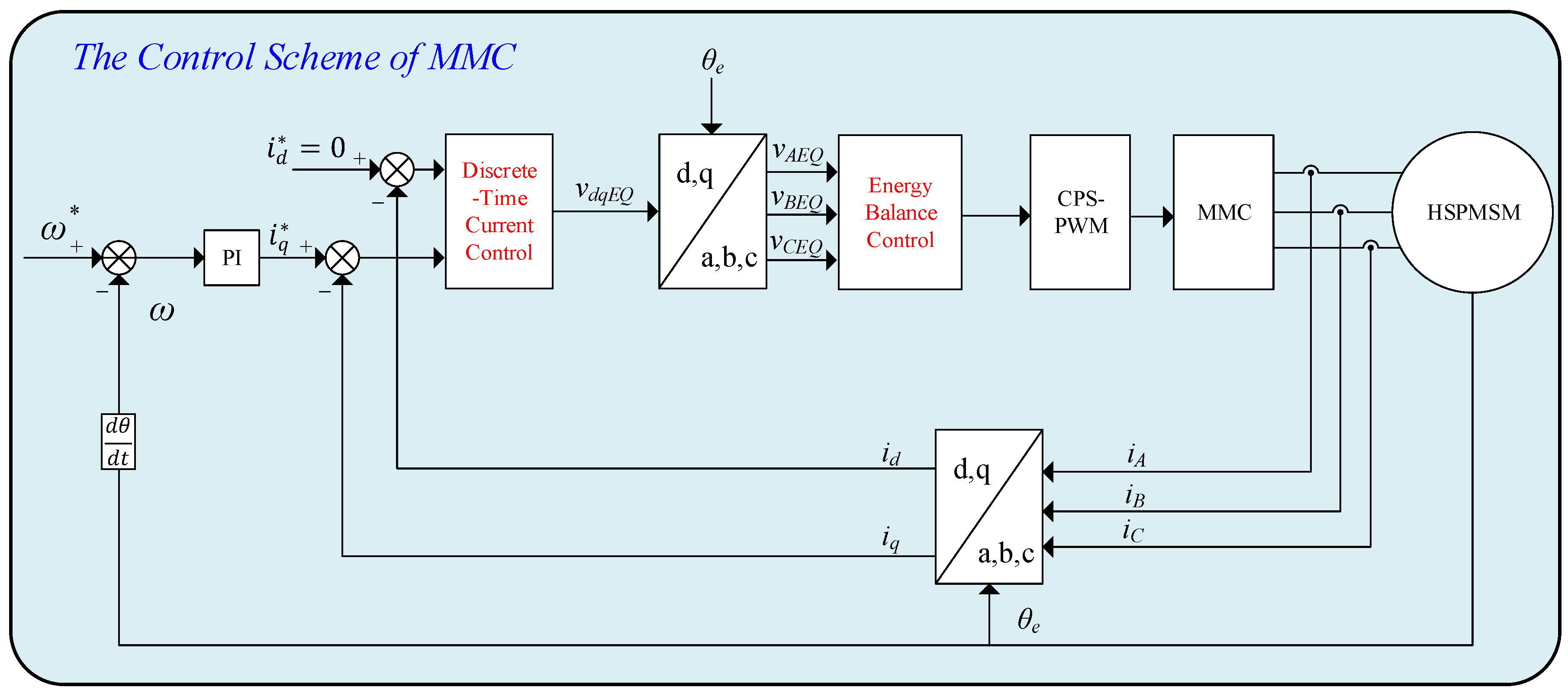
3. Discrete-Time Current Control Scheme

At first, the discrete-time model is illustrated in this section. Then, the conventional PI current regulator is analyzed. Finally, the discrete-time current regulator is designed.

3.1. Discrete-Time Model

By transforming (5) into $dq$ coordinates, the continuous-time domain state space equation of the bridge arm voltage and current under $dq$ coordinates are obtained as follows:

$$\begin{array}{c}\left[\begin{array}{c}\frac{d{i}_d}{dt}\\ \frac{d{i}_q}{dt}\end{array}\right]=\left[\begin{array}{cc}-\frac{R_s}{L_{eq}}& {\omega }_e\\ -{\omega }_e& -\frac{R_s}{L_{eq}}\end{array}\right]\left[\begin{array}{c}{i}_d\\ i_q\end{array}\right]+\left[\begin{array}{cc}\frac{1}{L_{eq}}& 0\\ 0& \frac{1}{L_{eq}}\end{array}\right]\left[\begin{array}{c}{v}_d-e_d\\ v_q-e_q\end{array}\right]\end{array}$$

(6)

where, ${\omega }_e$ is the electrical angular velocity of the MMC.

It is well known that the continuous-time state space equation is defined as

$$\begin{array}{cc}\hfill \dot{\mathit{x}}\left(t\right)& =\mathit{Ax}\left(t\right)+\mathit{Bu}\left(t\right)\hfill \end{array}$$

(7)

The state space equations of linear fixed-step discrete-time systems can be derived to obtain

$$\begin{array}{cc}\hfill \mathit{x}\left[\right(k+1\left)T\right]& =\mathit{G}\left(T\right)\mathit{x}\left(kT\right)+\mathit{H}\left(T\right)\mathit{u}\left(kT\right)\hfill \end{array}$$

(8)

where, T is sampling period, $\mathit{G}\left(T\right)$ and $\mathit{H}\left(T\right)$ are presented as follows:

$$\begin{array}{cc}\hfill \mathit{G}\left(T\right)& =e^{\mathit{A}T}\hfill \end{array}$$

(9)

$$\begin{array}{cc}\hfill \mathit{H}\left(T\right)& ={\int }_0^T{e}^{\mathit{A}T}\mathit{B}dt\hfill \end{array}$$

(10)

Thus, the discrete-time voltage and current model of (6) can be described as

$$\begin{array}{c}\left[\begin{array}{c}{i}_d\left[(k+1)T\right]\\ i_q\left[(k+1)T\right]\end{array}\right]=\mathit{G}\left(T\right)\left[\begin{array}{c}{i}_d\left(kT\right)\\ i_q\left(kT\right)\end{array}\right]+\mathit{H}\left(T\right)\left[\begin{array}{c}{v}_d\left(kT\right)-e_d\left(kT\right)\\ v_q\left(kT\right)-e_q\left(kT\right)\end{array}\right]\end{array}$$

(11)

According to (9) and (10),

$$\begin{array}{c}\mathit{G}\left(T\right)=\left[\begin{array}{cc}{e}^{-\frac{R_s}{L_{eq}}T}cos\left({\omega }_{e}T\right)& e^{-\frac{R_s}{L_{eq}}T}sin\left({\omega }_{e}T\right)\\ -e^{-\frac{R_s}{L_{eq}}T}sin\left({\omega }_{e}T\right)& e^{-\frac{R_s}{L_{eq}}T}cos\left({\omega }_{e}T\right)\end{array}\right]\end{array}$$

(12)

$$\begin{array}{c}\mathit{H}\left(T\right)=\left[\begin{array}{cc}{\sigma }_1& -{\sigma }_2\\ {\sigma }_2& {\sigma }_1\end{array}\right]\end{array}$$

(13)

where,

$$\left\{\begin{array}{cc}\hfill {\sigma }_1& =\frac{{\omega }_e{L}_{eq}Dsin\left({\omega }_{e}T\right)-R_{s}Dcos\left({\omega }_{e}T\right)+R_s}{{\omega }_e^2{L}_{eq}^2+R_s^2}\hfill \\ \hfill {\sigma }_2& =\frac{{\omega }_e{L}_{eq}Dcos\left({\omega }_{e}T\right)+R_{s}Dsin\left({\omega }_{e}T\right)-w_e{L}_{eq}}{{\omega }_e^2{L}_{eq}^2+R_s^2}\hfill \end{array}\right.$$

(14)

where,

$$\begin{array}{c}\hfill D=e^{-\frac{R_s}{L_{eq}}T}\end{array}$$

(15)

Similarly, define $f_{\alpha \beta }=f_{\alpha }+j·f_{\beta }$, the back EMF under $\alpha \beta$ coordinate is given by

$$\begin{array}{c}\frac{d}{dt}\left[\begin{array}{c}{i}_{\alpha \beta }\\ e_{\alpha \beta }\end{array}\right]=\left[\begin{array}{cc}-\frac{R_s}{L_{eq}}& -L_{eq}\\ 0& -j{\omega }_e\end{array}\right]\left[\begin{array}{c}{i}_{\alpha \beta }\\ e_{\alpha \beta }\end{array}\right]+\left[\begin{array}{cc}\frac{1}{L_{eq}}& 0\\ 0& 0\end{array}\right]\left[\begin{array}{c}{v}_{\alpha \beta }\\ 0\end{array}\right]\end{array}$$

(16)

Therefore, the discrete-time back EMF model in $dq$ rotating reference frame could be given by:

$$\left\{\begin{array}{cc}\hfill e_d\left(k\right)& =\frac{{\omega }_e{L}_{eq}cos\left({\omega }_{e}T\right)-D{\omega }_e{L}_{eq}-R_{s}sin\left({\omega }_{e}T\right)}{R_s^2+{\omega }_e^2{L}_{eq}^2}F\hfill \\ \hfill e_q\left(k\right)& =\frac{R_{s}cos\left({\omega }_{e}T\right)-D{R}_s-{\omega }_e{L}_{eq}sin\left({\omega }_{e}T\right)}{R_s^2+{\omega }_e^2{L}_{eq}^2}F\hfill \end{array}\right.$$

(17)

where,

$$\begin{array}{c}\hfill F=\frac{R_s}{1-e^{-\frac{R_s}{L_{eq}}T}}{\omega }_e{\psi }_{pm}\end{array}$$

(18)

3.2. Conventional PI Method

According to [29], the closed-loop transfer function of the conventional PI current regulator in complex plane is derived as follows:

$$\begin{array}{c}\hfill G_{loop}\left(z\right)=\frac{1-e^{-(R_s/L_{eq})T}}{R_s·z·e^{j{\omega }_{e}T}·(z·e^{j{\omega }_{e}T}-e^{-(R_s/L_{eq})T})}·(k_p+\frac{k_{i}T}{z-1}·\frac{z+1}{2})\end{array}$$

(19)

where, $k_p$ and $k_i$ are proportional and integral coefficients of the PI controller, respectively.

The complex planepole-zero map of the closed-loop transfer function with the variation in the running frequency from 0 to 600 Hz is demonstrated in Figure 3. It can be observed that with the increase in the electric frequency, the pole of the current regulator gradually moves upward to the circle and finally outside the unit circle in the right plane, the current loop loses its stability. Therefore, when the fundamental frequency of the system is over 400 Hz, the performance of the conventional PI controller is very poor, and even the closed-loop system oscillates and is unstable. Therefore, when the frequency is high, the conventional PI controller is not suitable for MMC drive systems, and a novel discrete-time current regulator should be designed.

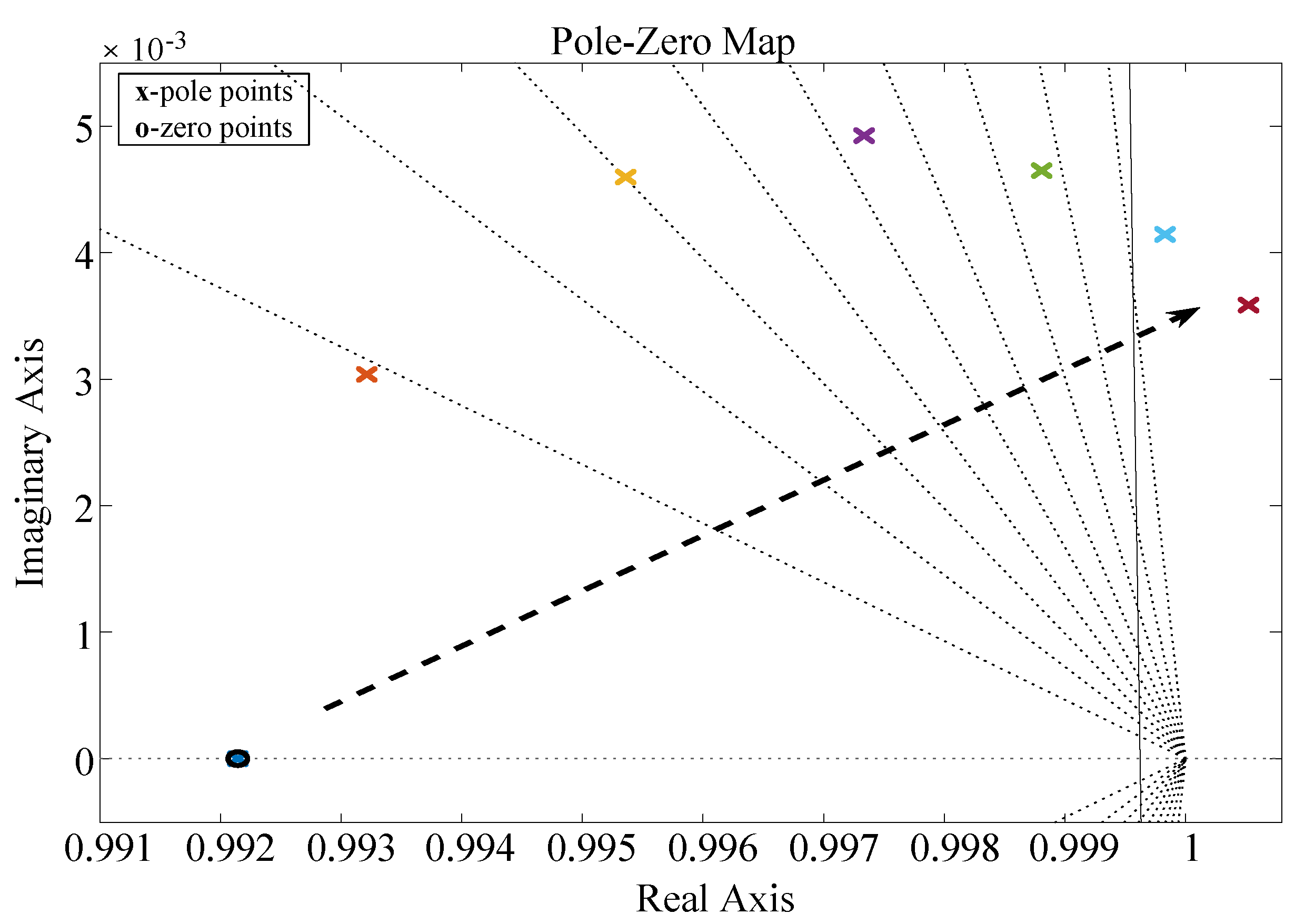
3.3. Controller Design of Discrete-Time Current

The output current should be satisfied as follows:

$$\begin{array}{c}\left[\begin{array}{c}{i}_d^{*}-i_d\left[(k+1)T\right]\\ i_q^{*}-i_q\left[(k+1)T\right]\end{array}\right]=K_c\left[\begin{array}{c}{i}_d^{*}-i_d\left(kT\right)\\ i_q^{*}-i_q\left(kT\right)\end{array}\right]\end{array}$$

(20)

where, $i_d^{*}$ and $i_q^{*}$ are reference current in $dq$ rotating reference frame, and $K_c$ is defined as the scale factor.

Therefore, the transfer function of (20) under z-domain is given by

$$\begin{array}{c}\hfill \frac{I_d\left(z\right)}{I_d^{*}\left(z\right)}=\frac{1-K_c}{z-K_c}\end{array}$$

(21)

For the purpose of keeping the stability of the discrete-time control system and to obtain a fast dynamic response, The scale factor $K_c$ should be set properly. In order to keep the pole location in the unit circle of complex plane, the $K_c$ should vary from 0.2 to 0.4.

According to (11), the discrete-time model is demonstrated as follows:

$$\begin{array}{cc}\hfill & \left[\begin{array}{c}{v}_d\left(kT\right)\\ v_q\left(kT\right)\end{array}\right]=\mathit{H}{\left(T\right)}^{-1}\left[\left[\begin{array}{c}{i}_d\left[(k+1)T\right]\\ i_q\left[(k+1)T\right]\end{array}\right]-\mathit{G}\left(T\right)\left[\begin{array}{c}{i}_d\left(kT\right)\\ i_q\left(kT\right)\end{array}\right]\right]\hfill \\ \hfill & +\left[\begin{array}{c}{e}_d\left(kT\right)\\ e_q\left(kT\right)\end{array}\right]\hfill \end{array}$$

(22)

Substituting (20) into (22), the discrete-time model at $(k+1)T$ is given by

$$\begin{array}{cc}\hfill & \left[\begin{array}{c}{v}_d\left[(k+1)T\right]\\ v_q\left[(k+1)T\right]\end{array}\right]=\mathit{H}{\left(T\right)}^{-1}\left[-\mathit{G}\left(T\right)\left[\begin{array}{c}{i}_d\left[(k+1)T\right]\\ i_q\left[(k+1)T\right]\end{array}\right]\right.\hfill \\ \hfill & -\left.K_c\left[\begin{array}{c}{i}_d^{*}-i_d\left[(k+1)T\right]\\ i_q^{*}-i_q\left[(k+1)T\right]\end{array}\right]+\left[\begin{array}{c}{i}_d^{*}\\ i_q^{*}\end{array}\right]\right]+\left[\begin{array}{c}{e}_d\left[(k+1)T\right]\\ e_q\left[(k+1)T\right]\end{array}\right]\hfill \end{array}$$

(23)

where,

$$\begin{array}{c}\mathit{H}{\left(T\right)}^{-1}=\left[\begin{array}{cc}{\delta }_1& {\delta }_2\\ -{\delta }_2& {\delta }_1\end{array}\right]\end{array}$$

(24)

where,

$$\left\{\begin{array}{cc}\hfill {\delta }_1& =\frac{D(R_{s}D-R_{s}cos\left({\omega }_{e}T\right)+{\omega }_e{L}_{eq}sin\left({\omega }_{e}T\right))}{1-2Dcos\left({\omega }_{e}T\right)+D^2}\hfill \\ \hfill {\delta }_2& =\frac{D(R_{s}sin\left({\omega }_{e}T\right)-{\omega }_e{L}_{eq}D+{\omega }_e{L}_{eq}cos\left({\omega }_{e}T\right))}{1-2Dcos\left({\omega }_{e}T\right)+D^2}\hfill \end{array}\right.$$

(25)

Finally, the proposed control scheme of MMC is depicted in Figure 4.

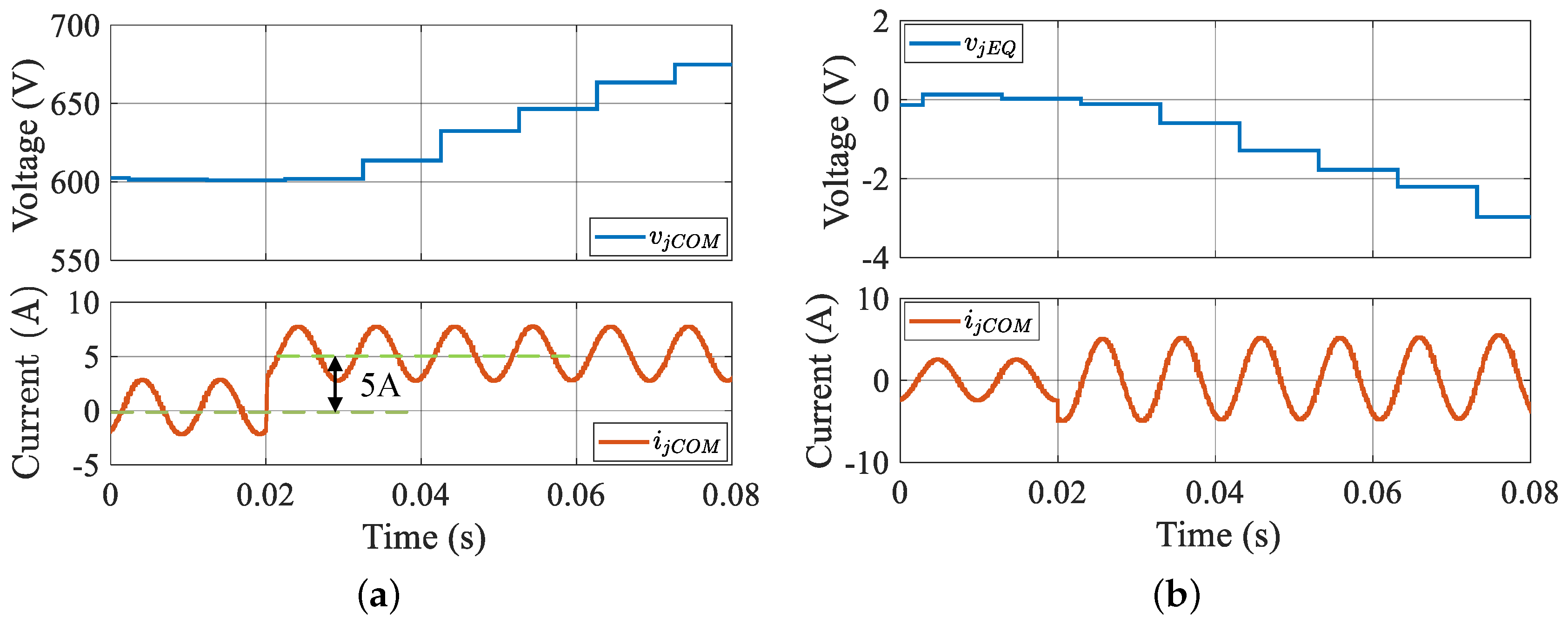
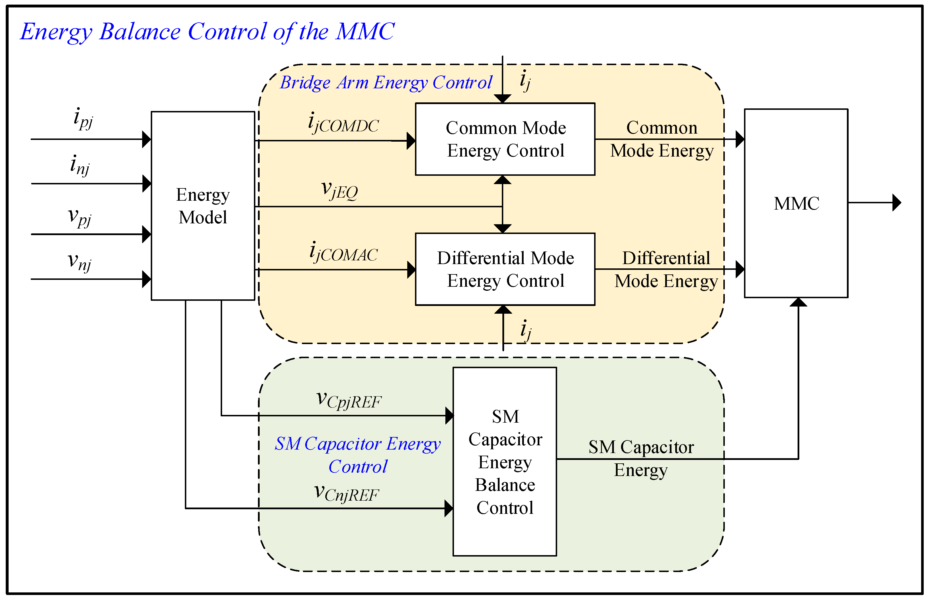
4. Energy Balance Control of the MMC

As mentioned in Section 1, the SM capacitor of the MMC has the problem of large voltage ripple in motor drives. Therefore, the energy balance models are established firstly in this section. Then, the design of energy balance controller is introduced.

4.1. Energy Model Analysis

Define

$$\left\{\begin{array}{cc}\hfill v_{jEQ}& =\frac{v_{nj}-v_{pj}}{2}\hfill \\ \hfill v_{jCOM}& =\frac{v_{nj}+v_{pj}}{2}\hfill \\ \hfill i_{jCOM}& =i_{pj}+i_{nj}\hfill \end{array}\right.$$

(26)

where $v_{jEQ}$($j=a,b,c$) is the equivalent bridge arm output voltage, $v_{jCOM}$($j=a,b,c$) is the common voltage of the MMC, and $i_{jCOM}$($j=a,b,c$) is defined as the circulating current.

Hence, Equations (1) and (5) can be rewritten as

$$\left\{\begin{array}{cc}\hfill v_{jEQ}& =R_s{i}_j+L_{eq}\frac{d{i}_j}{dt}+e_j-\frac{v_{DC}}{2}\hfill \\ \hfill v_{DC}& =2v_{jCOM}+L\frac{d{i}_{jCOM}}{dt}\hfill \end{array}\right.$$

(27)

4.2. SM Capacitor Energy Model

The SM capacitor voltage is presented as

$$\left\{\begin{array}{cc}\hfill C\frac{d{v}_{Cpjm}}{dt}& =i_{pj}\frac{v_{pjm}}{v_{Cpjm}}\hfill \\ \hfill C\frac{d{v}_{Cnjm}}{dt}& =i_{nj}\frac{v_{njm}}{v_{Cnjm}}\hfill \end{array}\right.$$

(28)

where, the SM capacitor voltages of the positive bridge arm is defined as $v_{Cpjm}$ ($m=1,2\dots$), and the negative bridge arm voltage of the SM capacitor is defined as $v_{Cnjm}$ ($m=1,2\dots$). Hence, the SM capacitor energy change ration is given as

$$\left\{\begin{array}{cc}\hfill \frac{d{E}_{Cpj}}{dt}& =i_{pj}{v}_{pj}\hfill \\ \hfill \frac{d{E}_{Cnj}}{dt}& =i_{nj}{v}_{nj}\hfill \end{array}\right.$$

(29)

Substituting (26) into (29), the positive arm and negative arm SM capacitor energy can be expressed as

$$\left\{\begin{array}{cc}\hfill \frac{d{E}_{Cpj}}{dt}& =\frac{1}{2}(i_{jCOM}+i_j)(v_{jCOM}-v_{jEQ})\hfill \\ \hfill & =\frac{1}{2}(i_{jCOM}{v}_{jCOM}+i_j{v}_{jCOM}-i_{jCOM}{v}_{jEQ}-i_j{v}_{jEQ})\hfill \\ \hfill \frac{d{E}_{Cnj}}{dt}& =\frac{1}{2}(i_{jCOM}-i_j)(v_{jCOM}+v_{jEQ})\hfill \\ \hfill & =\frac{1}{2}(i_{jCOM}{v}_{jCOM}-i_j{v}_{jCOM}+i_{jCOM}{v}_{jEQ}-i_j{v}_{jEQ})\hfill \end{array}\right.$$

(30)

Define

$$\left\{\begin{array}{cc}\hfill E_{CjSum}& =E_{Cpj}+E_{Cnj}\hfill \\ \hfill E_{CjDiff}& =E_{Cpj}-E_{Cnj}\hfill \end{array}\right.$$

(31)

where, $E_{CjSum}$($j=a,b,c$) is the common mode energy, and $E_{CjDiff}$($j=a,b,c$) is the differential mode energy. Thus, the (31) can be rewritten as

$$\left\{\begin{array}{cc}\hfill \frac{d{E}_{CjSum}}{dt}& =i_{jCOM}{v}_{jCOM}-i_j{v}_{jEQ}\hfill \\ \hfill \frac{d{E}_{CjDiff}}{dt}& =i_j{v}_{jCOM}-i_{jCOM}{v}_{jEQ}\hfill \end{array}\right.$$

(32)

4.3. Bridge Arm Energy Model

According to (32), the energy change ration is given as

$$\left\{\begin{array}{cc}\hfill \underset{0}{\overset{T}{\int }}\frac{d{E}_{CjSum}}{dt}& =\underset{0}{\overset{T}{\int }}{i}_{jCOM}{v}_{jCOM}dt-\underset{0}{\overset{T}{\int }}{i}_{jCOM}{v}_{jCOM}dt\hfill \\ \hfill \underset{0}{\overset{T}{\int }}\frac{d{E}_{CjDiff}}{dt}& =\underset{0}{\overset{T}{\int }}{i}_j{v}_{jCOM}dt-\underset{0}{\overset{T}{\int }}{i}_{jCOM}{v}_{jEQ}dt\hfill \end{array}\right.$$

(33)

Meanwhile, the output current $i_j$, the output voltage $v_{jEQ}$, the circulating current $i_{jCOM}$ and common voltage $v_{jCOM}$ can be defined as follows:

$$\left\{\begin{array}{cc}\hfill i_j& =i_{AC}sin\left({\omega }_{e}t\right)\hfill \\ \hfill v_{jEQ}& =v_{AC}sin({\omega }_{e}t+\psi )+v_{EQCOM}\hfill \\ \hfill i_{jCOM}& =i_{jCOMAC}sin({\omega }_{e}t+{\psi }_{com})+i_{jCOMDC}\hfill \\ \hfill v_{jCOM}& =\frac{v_{DC}}{2}-\frac{1}{2}{\omega }_{e}L{i}_{jCOMAC}cos({\omega }_{e}t+{\psi }_{com})\hfill \end{array}\right.$$

(34)

where $i_{AC}$ and $v_{AC}$ are the amplitude of the output current and voltage, respectively. And the common mode voltage is defined as $v_{EQCOM}$, $\psi$ is the power factor angle, ${\psi }_{com}$ is the power factor angle of common mode voltage.

Combining (33) and (34), the common mode energy change ration can be expressed as

$$\begin{array}{cc}\hfill \frac{d{E}_{CjSum}}{dT}& =i_{jCOMDC}\frac{v_{DC}}{2}-\frac{1}{2}{i}_{AC}{v}_{AC}cos\left(\psi \right)\hfill \end{array}$$

(35)

Similarly, the differential mode energy change ration is expressed as

$$\begin{array}{cc}\hfill \frac{d{E}_{CjDiff}}{dT}& =\frac{1}{2}{i}_{jCOMAC}{v}_{AC}sin({\psi }_{com}-(\psi +\frac{\pi }{2}))\hfill \end{array}$$

(36)

The waveforms of adjusting the common mode voltage and differential mode voltage are depicted in Figure 5. When $t=0.02$ s, $i_{jCOMDC}$ increases by 5 A, as shown in Figure 5a. $i_{jCOM}$ increases, $v_{jCOM}$ also increases with $i_{jCOM}$. Therefore, the common mode energy can be controlled by $i_{jCOMDC}$. When increasing the $i_{jCOMAC}$ at $t=0.02$ s, $i_{jCOM}$ also increases, the $v_{jEQ}$ in the balance gradually deviates from 0, which is shown in Figure 5b. It is illustrated in Figure 5b that the differential mode energy can be adjusted.

4.4. Energy Balance Controller Design

The control scheme of the energy balance control is depicted in Figure 6.

4.4.1. Control Scheme of Bridge Arm Energy

According to the results of Figure 5a, the DC component $i_{jCOMDC}$ of the circulating current $i_{jCOM}$ can control the the common mode energy, therefore, the common mode energy controller is given by:

$$\begin{array}{cc}\hfill i_{jCOMDCREF}& =K_{sumP}C\frac{1}{TN}(2v_{DC}-(v_{pj}+v_{nj}))+\frac{2P_j-{i_{AC}}^2\sqrt{{R_s}^2+{\left(\omega L_{eq}\right)}^2}sin\left(\psi \right)}{v_{dc}}\hfill \end{array}$$

(37)

where, $i_{jCOMDCREF}$ is the reference value of the $i_{jCOMDC}$, $K_{sumP}$ is the gain of common mode energy controller, $P_j=i_{jDC}{v}_{jDC}$, $i_{jDC}$ and $v_{jDC}$ are the DC components of output current and voltage, respectively.

According to the Figure 5b, the differential mode energy can be controlled by $i_{jCOMAC}$, the controller is presented as

$$\begin{array}{c}\hfill i_{jCOMACREF}=K_{Diff}C\frac{0-({v_{Cpj1DC}}^2+{v_{Cpj2DC}}^2+\cdots -{v_{Cnj1DC}}^2-{v_{Cnj2DC}}^2-\cdots )}{T{v}_{AC}}\end{array}$$

(38)

where, $i_{jCOMACREF}$ is the reference value of the $i_{jCOMAC}$

Combining (27) and (38), the circulating current is given by

$$\begin{array}{c}\hfill v_{jCOM}=\frac{1}{2}{v}_{DC}-K_{ICOM\_P}\frac{L}{2}\frac{i_{jCOMREF}-i_{jCOM}}{T}-\frac{L}{2}{\omega }_e{i}_{jCOMAC}cos({\omega }_{e}t+{\psi }_{com})\end{array}$$

(39)

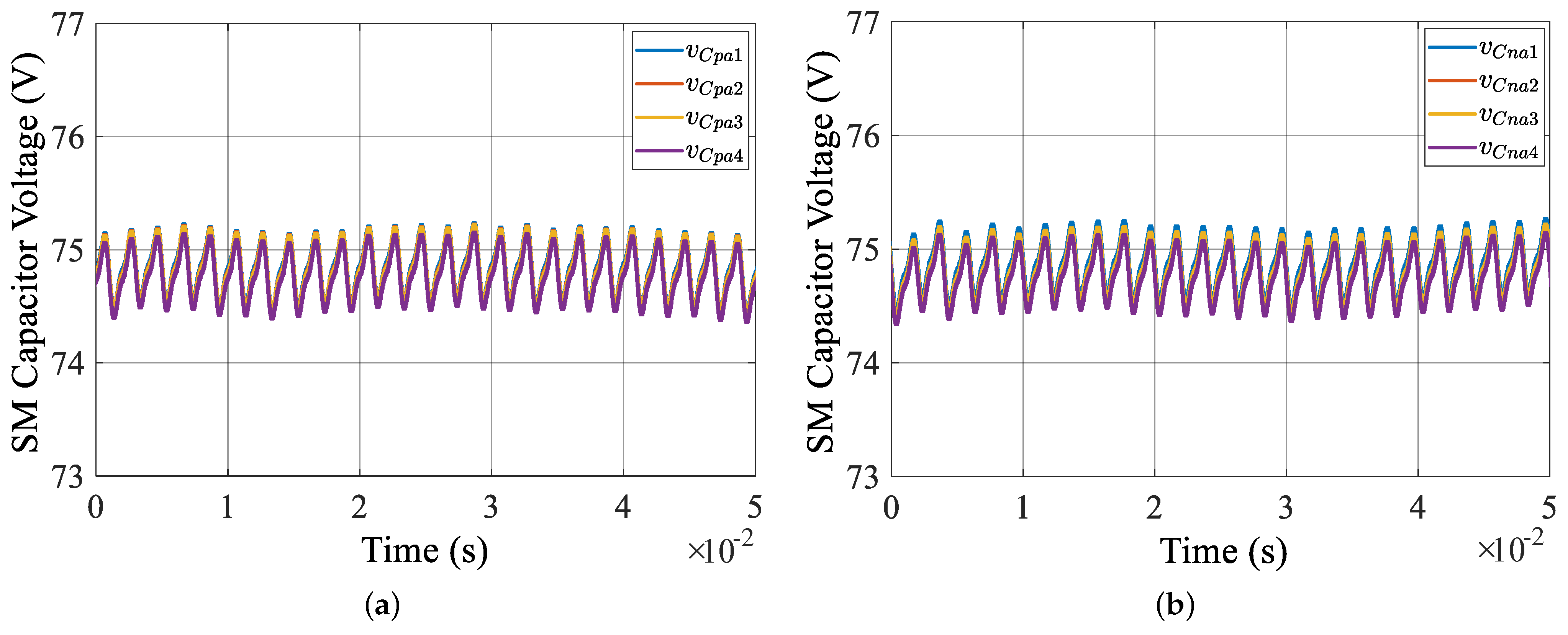
4.4.2. SM Capacitor Energy Control

In terms of (28), the SM capacitor voltage can be divided into

$$\left\{\begin{array}{cc}\hfill v_{pjm}& =\frac{v_{pj}}{N}+\Delta v_{pjm}\hfill \\ \hfill v_{njm}& =\frac{v_{nj}}{N}+\Delta v_{njm}\hfill \end{array}\right.$$

(40)

where, the SM capacitor’s increment value of the positive bridge arm is $\Delta v_{pjm}$ and the SM capacitor’s increment value of the negative bridge arm is $\Delta v_{njm}$. For the purpose of keeping the voltage balance of the SM capacitor, ${\sum }_{i=1}^N{v}_{pjm}$ and ${\sum }_{i=1}^N{v}_{njm}$ should be guaranteed to be 0.

The SM capacitor balance controller can be given by

$$\left\{\begin{array}{cc}\hfill i_{pj}{v}_{pjm}& =i_{pj}(\frac{v_{pj}}{N}+\Delta v_{pjm})=\frac{P_{pj}}{N}+K_p\frac{1}{2}\frac{{v_{CpjREF}}^2-{v_{Cpjm}}^2}{T}\hfill \\ \hfill i_{nj}{v}_{njm}& =i_{nj}(\frac{v_{nj}}{N}+\Delta v_{njm})=\frac{P_{nj}}{N}+K_p\frac{1}{2}\frac{{v_{CnjREF}}^2-{v_{Cnjm}}^2}{T}\hfill \end{array}\right.$$

(41)

where, $K_p$ is the gain of SM capacitor balance controller, $P_{pj}/N$ and $P_{nj}/N$ are the average power levels of the SM capacitor.

Assuming the $v_{Cp,njm}$ is around $v_{Cp,njREF}$, (41) can be simplified as follows:

$$\begin{array}{cc}\hfill \Delta v_{pjm}& \approx K_p\frac{1}{2}\frac{v_{CpjREF}}{i_{pj}}\frac{v_{CpjREF}-v_{Cpjm}}{T}\hfill \\ \hfill \Delta v_{njm}& \approx K_p\frac{1}{2}\frac{v_{CnjREF}}{i_{nj}}\frac{v_{CnjREF}-v_{Cnjm}}{T}\hfill \end{array}$$

(42)

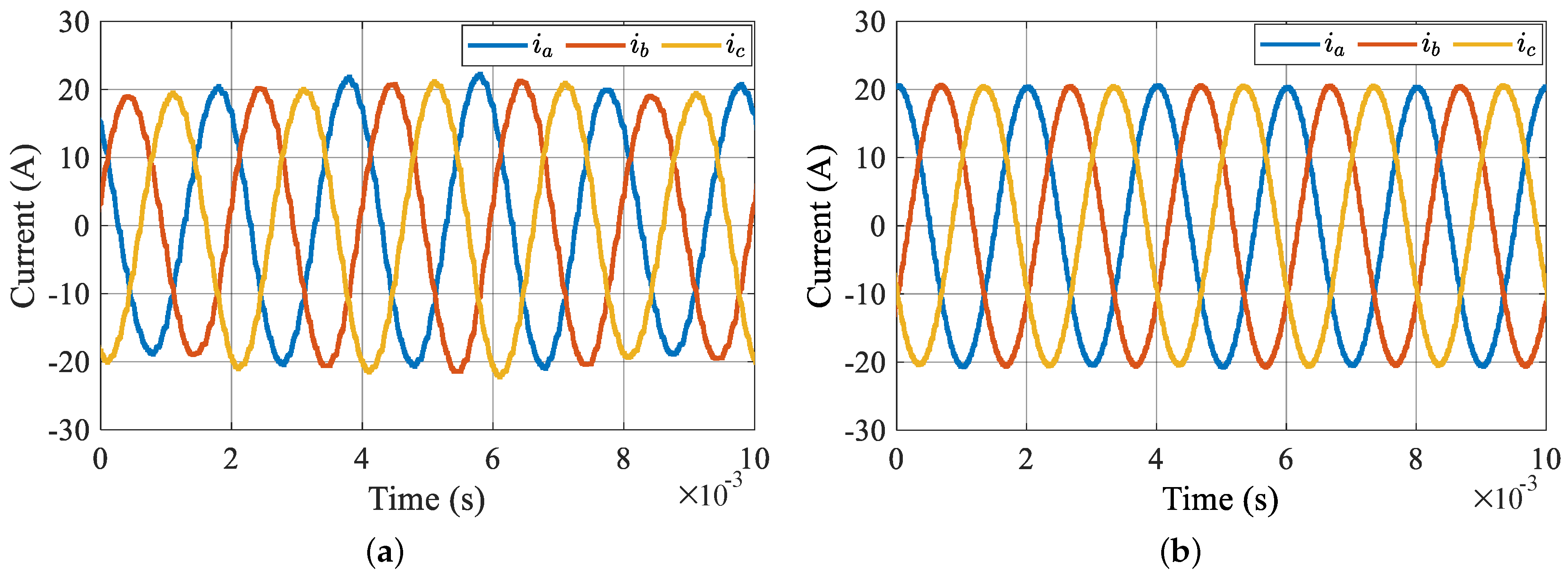
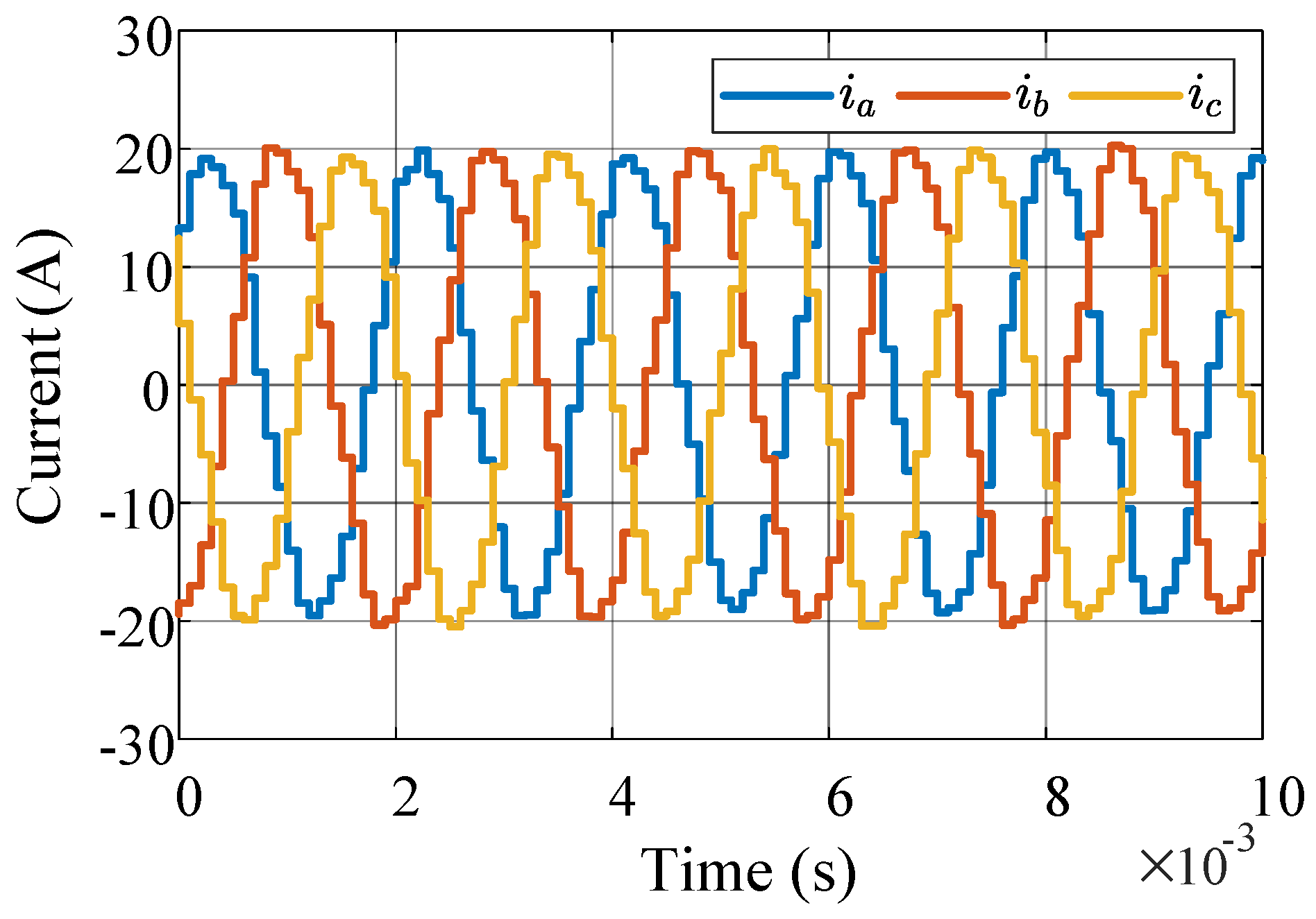
5. Simulation Analysis

In this section, a three-phase MMC for the HSPMM drive is performed in MATLAB/Simulink to verify the presented control method. The simulation and experimental parameters of the HSPMM and the MMC are drawn in

Table 1. Simulation and experimental parameters of the HSPMM.

Parameter	Symbol	Value
Rated mechanical speed	n	15 kr/min
Pole pairs	$p_n$	2
PM flux linkage	${\psi }_{pm}$	0.04 Wb
Rate current	I	20 A
Stator resistance	$R_s$	0.01385 $\mathsf{\Omega }$
Stator inductance	$L_d=L_q$	0.1256 mH

and

Table 2. Simulation and experimental parameters of the MMC.

Parameter	Symbol	Value
Number of SM per arm	N	4
Number of IGBT half bridge	/	24
Submodule capacitance	C	4 mF
DC voltage	$v_{DC}$	300 V
Bridge arm inductance	L	0.1 mH
Switching frequency	$f_s$	10 kHz

.

The comparison diagram of MMC three-phase current with different control methods is shown in Figure 7. At this time, the motor speed is 15 kr/min, and the system fundamental frequency reaches 500 Hz. Among them, Figure 7a is the output current of the MMC with the traditional PI discrete controller. The three-phase current of the MMC is unbalanced at high-speed, and there are large fluctuations in the current. The current waveform of the discrete-time current regulator is shown in Figure 7b, the three-phase current is in a steady state and is symmetrical.

The comparative simulation waveforms of the $dq$-axis current of MMC is shown in Figure 8. Figure 8a shows the waveform with a conventional PI discrete controller and Figure 8b shows the waveform with a discrete-time current regulator. Without considering the speed loop, the q-axis reference current jumps from 10 A to 20 A when the motor speed is increased from 10.5 kr/min (350 Hz) to 15 kr/min (500 Hz). From Figure 8, it is easy to observe that the d-axis current deviation of the traditional PI discrete regulator reaches up to 4 A, and the q-axis current overshoots up to 2.5 A with a longer response time. While the d-axis current deviation of the discrete-time current regulator is only about 0.4 A, the q-axis current overshoots are only about 1.1 A. The d-axis current deviation of the proposed discrete-time current regulator is only $10\%$ of the conventional PI regulator, and the q-axis current overshoots of the proposed discrete-time current regulator is only $44\%$ of the conventional PI regulator. And the response is fast, the q-axis current response of the proposed discrete-time current regulator is only $75\%$ of the conventional PI regulator. The above simulation results demonstrate that the discrete-time current regulator is able to track the reference value stably and has good dynamic effect.

Figure 9 describes the a-phase positive bridge arm SM capacitor voltage waveforms with the SM capacitor energy balance control. Firstly, the positive bridge SM capacitor is in a steady state under the SM capacitor energy control. When at 0.1 s, the system shuts down the SM capacitor energy balance control, and the SM capacitor voltage increases rapidly to an unstable state. Then, the system restarts the SM capacitor energy balance controller, the voltage decreases rapidly to about 75 V, and returns to a stable state. The simulation results show that the SM capacitor energy control has an excellent effect.

Figure 10 shows the positive and negative bridge arm SM capacitor voltage simulation waveform of MMC. It can be observed from Figure 10a,b that when the motor is running at a high speed of 15 kr/min (500 Hz), both the positive bridge arm and negative bridge arm SM capacitor voltage are maintained stably at 75 V.

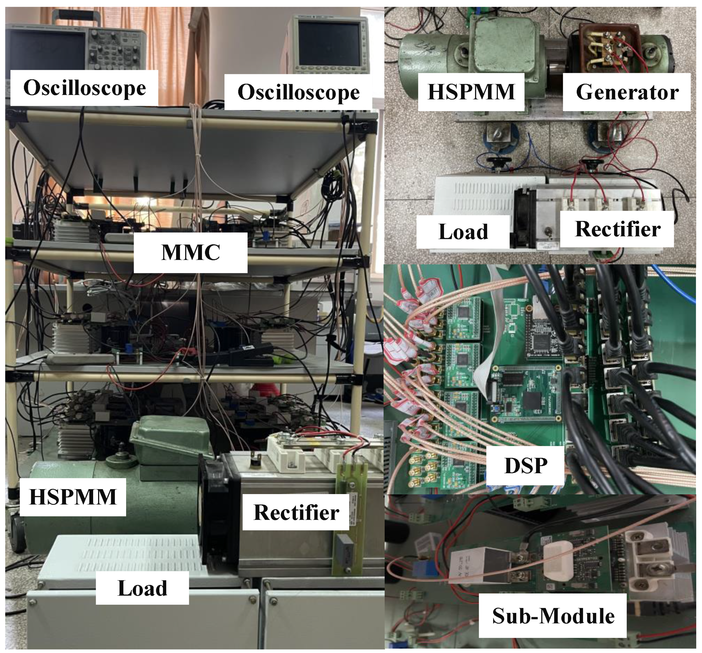
6. Experimental Verifications

To further verify the effectiveness of the proposed control method, the experimental setup is shown in Figure 11. The DC side is powered by a DC source, the AC side HSPMM connected to the generator in a pair-drag mode is driven by the MMC, and finally, the generator is connected to the resister load through a rectifier. The control board utilized the DSP TMS320F28379d to implement the proposed control method. The maximum system clock frequency of TMS320F28379D is 200 MHz. Thus, it is sufficient to solve the optimization problem in one sampling period. The control frequency is set as 10 kHz. Through the MATLAB/Simulink, the Embedded Coder module can easily generate the program code using the C language. Then, the generated C code can directly run in Ti DSP. The variables of the algorithm are able to be recorded on an external RAM and then be transferred to the PC for analysis through the Ethernet module integrated in the control board. The equivalent output switching frequency of MMC equals to $2n{f}_s=80$ kHz due to the carrier based phase-shifted PWM (CPS-PWM) technology being applied, which can boost the output switching frequency of MMC. And the specifications of IGBT half-bridge module is 600 V/200 A. The experimental parameters of the tested MMC for the HSPMM have already been drawn in Table 1 and Table 2.

As shown in Figure 12, the experimental output current waveforms of the MMC with a high-speed permanent magnet motor at 15 kr/min (500 Hz), the experimental results show that with the MMC system using the discrete-time current regulator, the three-phase current of the MMC is stable and symmetrical, and the motor is in the steady state, which further proves the effectiveness of the discrete-time current regulator.

When the q-axis reference current is stepped, the dynamic performance of the experimental waveform diagram of the current controller is shown in Figure 13, and there is no speed loop set in the control system at this time. In Figure 13a, the q-axis reference current steps from 15 A to 18 A in 0.8 s. The rise time of the q-axis current is about 2.8 ms, the overshoot is about 1 A, and the d-axis reference current is 0, and the maximum deviation of the d-axis current is about 0.27 A. Under the action of the q-axis current, the motor gradually rises from 9.6 kr/min (320 Hz) to 12.8 kr/min (420 Hz). Figure 13b shows the experimental waveform of the q-axis reference current from 18 A to 20 A. The rise time of the q-axis current is about 2 ms, the overshoot is about 1.4 A, and the maximum deviation value of the d-axis current is about 0.4 A. The high-speed PM motor rises from 12.8 kr/min (420 Hz) to the rated speed of 15 kr/min (500 Hz). Based on the results of the dynamic performance of the current controller, the effectiveness of the discrete-time current regulator proposed in this paper can be proven. And the current loop controller can quickly track the current change when the reference current is stepped, and has strong dynamic performance. The discrete-time current regulator can quickly adjust the current to the reference value and still has good dynamic characteristics at high frequencies, ensuring that the motor can quickly adjust speed and maintain stability during high-speed operation.

Figure 14 shows the SM capacitor voltage waveform of MMC. When the motor is running at 15 kr/min (500 Hz), it can be observed that both the positive and negative bridge arm SM capacitor voltage are maintained at 75 V stably from Figure 14a,b, and the SM capacitor voltage pulsation is only about 1 V. The experimental results prove that the energy balance control method of MMC achieves significant performance.

Figure 15 shows the bridge arm current of MMC. The bridge arm current running at 15 kr/min 500 Hz contains the DC components and AC components. The three-phase bridge arm current is symmetrical.

7. Conclusions

This article presents a new discrete-time current control method for the MMC in the HSPMM drive application. The symmetrical discrete-time model of the MMC is established. To overcome the poor performance of the conventional PI controller at high frequency, the novel discrete-time current regulator is designed. Then, the energy balance models of MMC are described, the energy balance control scheme which is suitable for MMC-based HSPMM is introduced. The performance of the proposed discrete-time current control method under both dynamic and steady states is validated by the simulation and experiment. The verification results show that the discrete-time current regulator for the MMC achieves significant performance. The d-axis and q-axis current overshoots of the proposed discrete-time current regulator are decreased, and the q-axis current rapidly responds. The experimental maximum motor speed is up to 15 kr/min (500 Hz). Moreover, the energy balance control of the MMC also ensures that the SM capacitor voltages are in balance. The voltage fluctuations were kept small at high frequencies.

References

1. Gerada, D.; Mebarki, A.; Brown, N.; Gerada, C.; Cavagnino, A.; Boglietti, A. High-Speed Electrical Machines: Technologies, Trends, and Developments. IEEE Trans. Ind. Electron. 2014, 61, 2946–2959. [Google Scholar] [CrossRef]
2. Lusignani, D.; Barater, D.; Franceschini, G.; Buticchi, G.; Galea, M.; Gerada, C. A high-speed electric drive for the more electric engine. In Proceedings of the 2015 IEEE Energy Conversion Congress and Exposition (ECCE), Montreal, QC, Canada, 20–24 September 2015; pp. 4004–4011. [Google Scholar] [CrossRef]
3. Zhao, N.; Zhu, Z.Q.; Liu, W. Rotor Eddy Current Loss Calculation and Thermal Analysis of Permanent Magnet Motor and Generator. IEEE Trans. Magn. 2011, 47, 4199–4202. [Google Scholar] [CrossRef]
4. Dong, J.; Huang, Y.; Jin, L.; Lin, H. Comparative Study of Surface-Mounted and Interior Permanent-Magnet Motors for High-Speed Applications. IEEE Trans. Appl. Supercond. 2016, 26, 5200304. [Google Scholar] [CrossRef]
5. Perisse, F.; Werynski, P.; Roger, D. High frequency behavior of AC machine: Application of turn insulation aging diagnostic. In Proceedings of the Conference Record of the 2006 IEEE International Symposium on Electrical Insulation, Toronto, ON, Canada, 11–14 June 2006; pp. 555–559. [Google Scholar] [CrossRef]
6. Wada, K.; Tsuji, K.; Muto, H.; Yashiro, O. Effect of cabling and grounding configuration on surge voltages in inverter-fed motors. In Proceedings of the 2006 IEEE Conference on Electrical Insulation and Dielectric Phenomena, Kansas City, MO, USA, 15–18 October 2006; pp. 602–606. [Google Scholar] [CrossRef]
7. Narayanasamy, B.; Sathyanarayanan, A.S.; Luo, F.; Chen, C. Reflected Wave Phenomenon in SiC Motor Drives: Consequences, Boundaries, and Mitigation. IEEE Trans. Power Electron. 2020, 35, 10629–10642. [Google Scholar] [CrossRef]
8. Langmaack, N.; Balasubramanian, S.; Mallwitz, R.; Henke, M. Comparative Analysis of High Speed Drive Inverter Designs using different Wide-Band-Gap Power Devices. In Proceedings of the 2021 23rd European Conference on Power Electronics and Applications (EPE’21 ECCE Europe), Ghent, Belgium, 6–10 September 2021; pp. 1–10. [Google Scholar] [CrossRef]
9. Chang, L.; Alvi, M.; Lee, W.; Kim, J.; Jahns, T.M. Efficiency Optimization of PWM-Induced Power Losses in Traction Drive Systems with IPM Machines Using Wide Bandgap-Based Inverters. IEEE Trans. Ind. Appl. 2022, 58, 5635–5649. [Google Scholar] [CrossRef]
10. Xu, Y.; Yuan, X.; Ye, F.; Wang, Z.; Zhang, Y.; Diab, M.; Zhou, W. Impact of High Switching Speed and High Switching Frequency of Wide-Bandgap Motor Drives on Electric Machines. IEEE Access 2021, 9, 82866–82880. [Google Scholar] [CrossRef]
11. Hatua, K.; Jain, A.K.; Banerjee, D.; Ranganathan, V.T. Active Damping of Output Filter Resonance for Vector-Controlled VSI-Fed AC Motor Drives. IEEE Trans. Ind. Electron. 2012, 59, 334–342. [Google Scholar] [CrossRef]
12. Yao, Y.; Peng, F.; Huang, Y. Position and Capacitor Voltage Sensorless Control of High-Speed Surface-Mounted PMSM Drive with Output Filter. In Proceedings of the 2018 IEEE Energy Conversion Congress and Exposition (ECCE), Portland, OR, USA, 23–27 September 2018; pp. 2374–2381. [Google Scholar] [CrossRef]
13. Wang, M.; Xu, Y.; Zou, J. Sliding mode control with open-switch fault diagnosis and sensorless estimation based on PI observer for PMSM drive connected with an LC filter. IET Power Electron. 2020, 13, 2334–2341. [Google Scholar] [CrossRef]
14. Yao, Y.; Huang, Y.; Peng, F.; Dong, J.; Zhu, Z. Discrete-Time Dynamic-Decoupled Current Control for LCL-Equipped High-Speed Permanent Magnet Synchronous Machines. IEEE Trans. Ind. Electron. 2022, 69, 12414–12425. [Google Scholar] [CrossRef]
15. Kouro, S.; Malinowski, M.; Gopakumar, K.; Pou, J.; Franquelo, L.G.; Wu, B.; Rodriguez, J.; Perez, M.A.; Leon, J.I. Recent Advances and Industrial Applications of Multilevel Converters. IEEE Trans. Ind. Electron. 2010, 57, 2553–2580. [Google Scholar] [CrossRef]
16. Raju, M.N.; Sreedevi, J.; Mandi, R.P.; Meera, K.S. Modular multilevel converters technology: A comprehensive study on its topologies, modelling, control and applications. IET Power Electron. 2019, 12, 149–169. [Google Scholar] [CrossRef]
17. Picas, R.; Zaragoza, J.; Pou, J.; Ceballos, S.; Konstantinou, G.; Capella, G.J. Study and Comparison of Discontinuous Modulation for Modular Multilevel Converters in Motor Drive Applications. IEEE Trans. Ind. Electron. 2019, 66, 2376–2386. [Google Scholar] [CrossRef]
18. Ke, Z.; Pan, J.; Sabbagh, M.A.; Na, R.; Zhang, J.; Wang, J.; Xu, L. Capacitor Voltage Ripple Estimation and Optimal Sizing of Modular Multi-Level Converters for Variable-Speed Drives. IEEE Trans. Power Electron. 2020, 35, 12544–12554. [Google Scholar] [CrossRef]
19. Li, B.; Han, L.; Mao, S.; Zhou, S.; Qu, Z.; Xu, D. Decoupled Modulation Scheme for Modular Multilevel Converters in Medium-Voltage Applications. IEEE Trans. Power Electron. 2020, 35, 11430–11441. [Google Scholar] [CrossRef]
20. Li, B.; Zhang, Y.; Wang, G.; Sun, W.; Xu, D.; Wang, W. A Modified Modular Multilevel Converter with Reduced Capacitor Voltage Fluctuation. IEEE Trans. Ind. Electron. 2015, 62, 6108–6119. [Google Scholar] [CrossRef]
21. Dekka, A.; Wu, B.; Zargari, N.R.; Fuentes, R.L. Dynamic Voltage Balancing Algorithm for Modular Multilevel Converter: A Unique Solution. IEEE Trans. Power Electron. 2016, 31, 952–963. [Google Scholar] [CrossRef]
22. Kolluri, S.; Gorla, N.B.Y.; Panda, S.K. Capacitor Voltage Ripple Suppression in a Modular Multilevel Converter Using Frequency-Adaptive Spatial Repetitive-Based Circulating Current Controller. IEEE Trans. Power Electron. 2020, 35, 9839–9849. [Google Scholar] [CrossRef]
23. Samajdar, D.; Bhattacharya, T. Capacitor Voltage Ripple Optimization in Modular Multilevel Converter Using Synchronous Reference Frame Energy Ripple Controller. IEEE Trans. Power Electron. 2022, 37, 7883–7895. [Google Scholar] [CrossRef]
24. Kumar, Y.S.; Poddar, G. Balanced Submodule Operation of Modular Multilevel Converter-Based Induction Motor Drive for Wide-Speed Range. IEEE Trans. Power Electron. 2020, 35, 3918–3927. [Google Scholar] [CrossRef]
25. Zhao, F.; Xiao, G.; Zhu, T.; Zheng, X.; Wu, Z.; Zhao, T. A Coordinated Strategy of Low-Speed and Start-Up Operation for Medium-Voltage Variable-Speed Drives with a Modular Multilevel Converter. IEEE Trans. Power Electron. 2020, 35, 709–724. [Google Scholar] [CrossRef]
26. Pan, J.; Ke, Z.; Al Sabbagh, M.; Li, H.; Potty, K.A.; Perdikakis, W.; Na, R.; Zhang, J.; Wang, J.; Xu, L. 7-kV 1-MVA SiC-Based Modular Multilevel Converter Prototype for Medium-Voltage Electric Machine Drives. IEEE Trans. Power Electron. 2020, 35, 10137–10149. [Google Scholar] [CrossRef]
27. Pan, J.; Ke, Z.; Li, X.; Zhao, Y.; Zhang, J.; Wang, J.; Xu, L. Integrated Control and Performance Analysis of High-Speed Medium-Voltage Drive Using Modular Multilevel Converter. IEEE J. Emerg. Sel. Top. Power Electron. 2023, 11, 3692–3704. [Google Scholar] [CrossRef]
28. Xia, T.; Peng, F.; Huang, Y. A Novel Energy Balance Control Method for a Modular Multilevel Converter in a High-Speed PMSM Drive Application. Energies 2023, 16, 5022. [Google Scholar] [CrossRef]
29. Bae, B.H.; Sul, S.K. A compensation method for time delay of full-digital synchronous frame current regulator of PWM AC drives. IEEE Trans. Ind. Appl. 2003, 39, 802–810. [Google Scholar] [CrossRef]
Figure 1. The topology structure of the MMC for HSPMM.
Symmetry 16 00200 g001
Figure 2. Circuit configuration of the MMC for HSPMM.
Symmetry 16 00200 g002
Figure 3. Pole−zero map of the current regulator.
Symmetry 16 00200 g003
Figure 4. The control scheme of MMC.
Symmetry 16 00200 g004
Figure 5. Waveforms of voltage: (a) common mode voltage, and (b) differential mode voltage.
Symmetry 16 00200 g005
Figure 6. Proposed energy balance control scheme.
Symmetry 16 00200 g006
Figure 7. Three-phase current: (a) conventional PI discrete regulator, and (b) discrete-time current regulator.
Symmetry 16 00200 g007
Figure 8. d q -axis current: (a) conventional PI regulator, and (b) discrete-time current regulator.
Symmetry 16 00200 g008
Figure 9. Validation the SM capacitor energy balance controller.
Symmetry 16 00200 g009
Figure 10. SM capacitor voltage: (a) simulated positive bridge arm, and (b) simulated negative bridge arm.
Symmetry 16 00200 g010
Figure 11. Experimental setup of the MMC.
Symmetry 16 00200 g011
Figure 12. Output current waveforms of the MMC.
Symmetry 16 00200 g012
Figure 13. Dynamic performance of the current controller: (a) the q-axis reference current steps from 15 A to 18 A, and (b) the q-axis reference current from 18 A to 20 A.
Symmetry 16 00200 g013
Figure 14. SM capacitor voltage: (a) positive, and (b) negative.
Symmetry 16 00200 g014
Figure 15. The bridge arm current of MMC: (a) phase-a, (b) phase-b, and (c) phase-c.
Symmetry 16 00200 g015