Abstract
This research work focuses on -Szász–Mirakjan operators coupling generalized beta function. The kernel functions used in -Szász operators often possess even or odd symmetry. This symmetry influences the behavior of the operator in terms of approximation and convergence properties. The convergence properties, such as uniform convergence and pointwise convergence, are studied in view of the Korovkin theorem, the modulus of continuity, and Peetre’s K-functional of these sequences of positive linear operators in depth. Further, we extend our research work for the bivariate case of these sequences of operators. Their uniform rate of approximation and order of approximation are investigated in Lebesgue measurable spaces of function. The graphical representation and numerical error analysis in terms of the convergence behavior of these operators are studied.
Keywords:
rate of convergence; mathematical operators; Szász operators; symmetric operators; Korovkin theorem; Lebesgue spaces; approximation algorithms; order of approximation MSC:
41A25; 41A27; 41A35; 41A36; 41A45
1. Introduction
Szász [1] presented a generalization of Bernstein polynomials [2] to investigate approximation properties on unbounded intervals, i.e., as follows:
where and
These operators are introduced in the 1950s and have been extensively studied by mathematicians over the years to achieve the flexibility in the approximation properties. The symmetry of the kernel affects how well Szász operators can approximate functions. Symmetric kernels tend to preserve certain functional forms or properties of functions being approximated, leading to specific convergence behaviors. Many mathematicians constructed various sequences of operators based on the classical Szász–Mirakjan operators given by (1). Recently, various scientists are working in the other branches of sciences like medical science, robotics, computer science, and others [3,4,5,6,7] in terms of these types of sequences of linear positive operators. In the recent past, several mathematicians contributed a healthy literature in approximation theory via linear positive operators, viz. Braha et al. [8], Özger et al. [9], Ansari et al. [10], Khan et al. [11], Acar et al. [12], Alotaibi [13], Mohiuddine et al. [14], Nasiruzzaman et al. [15], Çiçek et al. [16], Cai et al. [17], Aslan et al. [18,19], and Izgi [20]. In continuation, Qi et al. [21] presented Szász–Mirakjan operators based on shape parameter as follows:
where
Many generalizations are investigated for the operators is given by (2), viz. Özger et al. [9] constructed a sequence of Kantorovich variants of -Schurer operators to approximate Lebesgue measurable class. For and , the functional (see [22]), , is given by
where
and
Rao et al. [23] introduced a sequence of classical Szász operators, coupling generalized beta function as follows:
Motivated with the above development of the literature, we construct a new sequence of Szász operators coupling generalized beta function:
where and are defined in Equations (3) and (4), respectively. Szász operators, named after the mathematician Gabor Sász, are a class of linear positive operators used in approximation theory and functional analysis. They are typically associated with the properties of symmetry and positivity. Here’s how they relate to symmetry:
Definition and symmetry: Szász operators are constructed using a kernel that exhibits certain symmetrical properties, such as being symmetric or involving symmetric functions. Symmetry in the context of Szász operators can refer to properties such as the following:
Evenness or oddness: The kernel functions used in Szász operators often possess even or odd symmetry. This symmetry influences the behavior of the operator in terms of approximation and convergence properties. Approximation properties: The symmetry of the kernel affects how well Szász operators can approximate functions. Symmetric kernels tend to preserve certain functional forms or properties of functions being approximated, leading to specific convergence behaviors.
Functional analysis perspective: in functional analysis, the symmetry of operators like Szász operators can be studied in terms of their action on function spaces and the preservation of certain structural properties under approximation.
Applications: understanding the symmetry properties of Szász operators is crucial in applications ranging from numerical analysis to signal processing, where approximating functions with known symmetries or preserving symmetrical properties is important.
In summary, Szász operators exhibit symmetry through their construction and the properties of their kernel functions, impacting their approximation capabilities and their role in functional analysis contexts.
Now, to derive the lemmas for the approximation results of sequences of operators given in (7), we consider test functions and the central moments as and , . To present this research work, it is divided into some sections. Sections one and two hold for the introductory and preliminary parts of this research work. In sections three and four, approximation theorems and graphical analysis are investigated. In the last two sections, we study the bivariate version of the operators given in (7), and their numerical graphical analysis is discussed.
2. Some Estimates and Approximation Results
Lemma 1
Lemma 2.
Let be given by (7). We have
Proof.
For , then
For , then
If , then
□
Lemma 3.
Let . Using Lemma 2, one can easily calculate the central moments of Szász–Mirakjan coupling generalized Beta operators as follows:
Definition 1
([24]). Let be the modulus of continuity. Then, for continuous function ℏ defined on closed interval we have
For and and , we obtain
Theorem 1.
For the operators defined by (7) and for every is convergent as , then , where ⇉ denotes the uniform convergence.
Proof.
By Krovkin-type property of Theorem in [25], it is enough to show that for . By Lemma 2, it is clear as and for
Similarly, for , . Hence, we arrived at the desired proof of Theorem 1. □
Theorem 2.
For and given by (7), we have
Proof.
In direction of the relation (8), we obtain
Choosing completes the proof of Theorem 2. □
3. Graphical and Numerical Analysis
In this section, we examine the convergence behavior of the operator defined by (7).
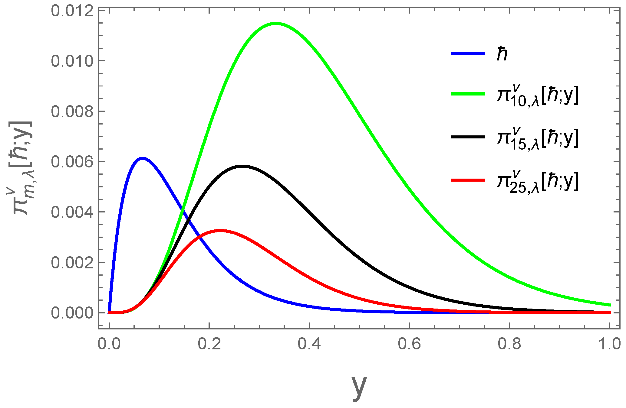
Example 1.

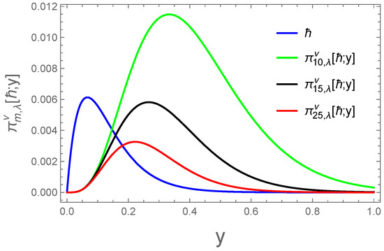

(a) For the function to analyze the numerical behavior of the operator (7), we compute the error using the formula
Dor different values of s, specifically 10, 15, and 25, for a fix values of . Then, Table 1 provides the numerical error values for the chosen parameters. Furthermore, Figure 1 and Figure 2 graphically illustrate the convergence behavior and the error approximation of the operator (7) for the same function and the parameter values
Table 1.
The error approximation of operators for 10, 15, 25.
Figure 1.
Convergence of operator for .
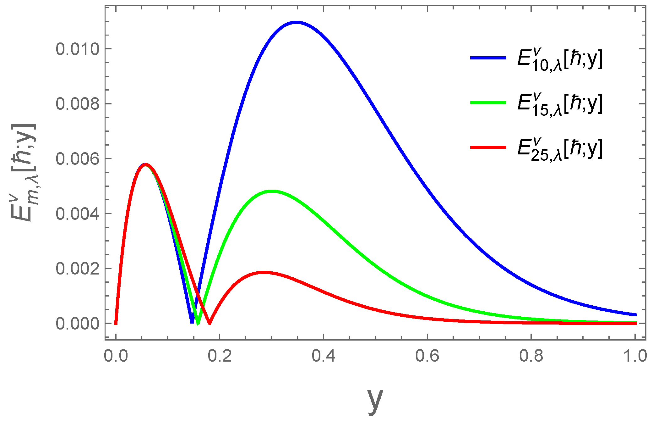
Figure 2.
Error approximation .
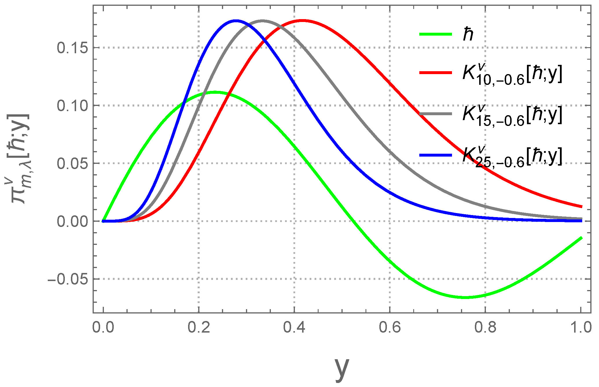
Example 2.
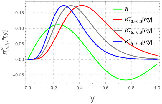
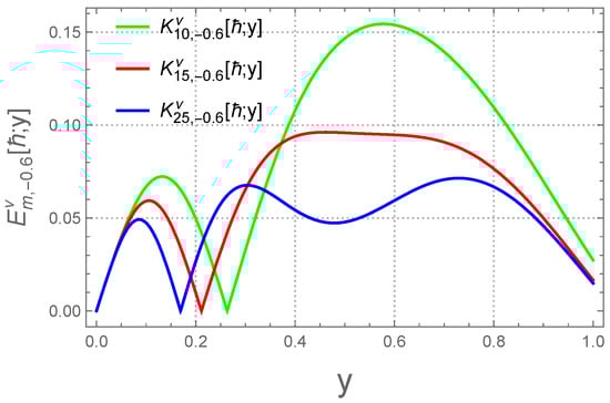
(b) For the function To analyze the numerical behavior of the operator (7), for the different value of and the same value of Table 2 illustrates the numerical behavior for the different values of with the help of and . Figure 3 and Figure 4 show the convergence behavior of the operators (7).
Table 2.
The error approximation of operators for 10, 15, 25.
Figure 3.
Convergence of operator for .
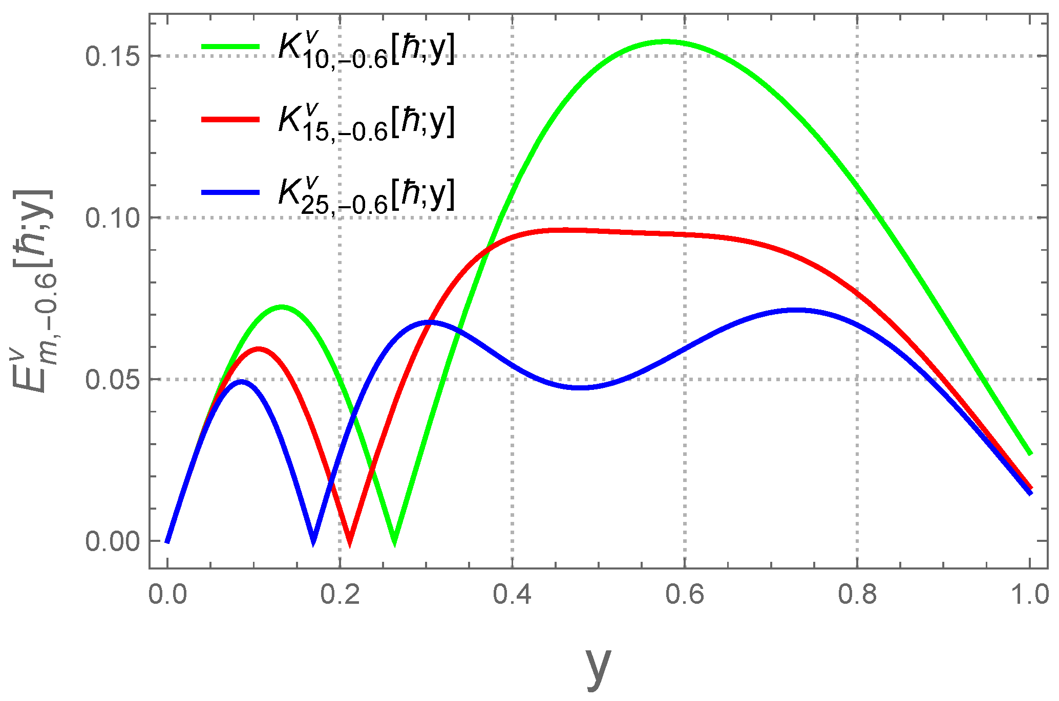
Figure 4.
Error approximation .
4. Local Approximation
In this section, we discuss direct approximation results for endowed with the norm. For any . For any and Peetre’s K-functional is given as
where .
By DeVore and Lorentz ([24] p. 177, Theorem ), there exist such that
Second-order modulus of continuity and is given as
Now, we consider the auxiliary operator as
Lemma 4.
Let and . Then, we obtain
where
Proof.
where
In the light of auxiliary operators defined in (10), we yield
In view of Taylor’s series expansion, for we obtain
Apply the auxiliary operators in the above Equation (10), we yield
On account of (10) and (11), we obtain
Theorem 3.
Let Then, we have
where is found in Lemma 4 and .
Proof.
For , and the auxiliary operator , we have
From Lemma 4 and Equation (11), we yield
Using Peetre’s K-functional, we have
Hence, we completes the proof of Theorem 3. We recall Lipschitz-type space here [26] as
where is a fixed constant and . , , are two real values. □
Theorem 4.
Proof.
First, we consider and we yield
It is obvious that
Therefore one has
In the light of Hlder’s inequality, Theorem 4, holds good for , with and , we yield
Since we yield
Hence, we arrived at our desired result. Now, we recall term order Lipschitz-type maximal function suggested by Lenze [27] as
and . □
Theorem 5.
Let and . Then, for all , one has
Proof.
We have
In the direction of Equation (17), we have
Using Hlder’s inequality with and , we have
we arrived at our desired result. □
5. Bivariate Extension of Generalized Beta Type -Szász–Mirakjan Operators
Take and represents a class of continuous functions over influenced with norm Then, for all and we introduced a bivariate extension as
where
and
for and
Lemma 5.
Proof.
In the direction linearity property and (2), we have
□
Lemma 6.
For for then we have following equalities:
Proof.
In the light of Lemma 5 and linearity property, one can easily prove the required result. □
Now, we prove the rate of convergence and order of approximation.
Definition 2.
Consider as given intervals and Then, for present the total modulus of continuity is defined as provided that and defined by
is termed as the total modulus of continuity corresponding to the function ℏ.
Here, we discuss the convergence rate of the operators given by (9). To discuss convergence rate, we revisit the following result presented by Volkov [28]:
Theorem 6.
Let be linear positive operators. If
and
uniformly on , then the sequence converges to ℏ uniformly on for any .
Theorem 7.
Let be the test functions restricted on . If
and
uniformly on , then
uniformly for all .
Proof.
In view of Lemma 5, it is evident for
For , , we obtain
Similarly
and in the light Lemma (5), we obtain
In the direction Theorem 6, Theorem 7 is easily proved. □
In the last result, we deal approximation order of the sequence of operators given by (9) as
Theorem 8
([29]). Let be a linear positive operator. For any , any and any , the following inequality
holds.
Theorem 9.
For and , and , one has
where and .
Proof.
From Theorem 8, we have
Selecting and , we arrive at the required result. □
6. Bivariate Graphical Analysis
Example 3.

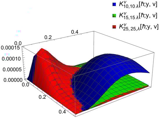
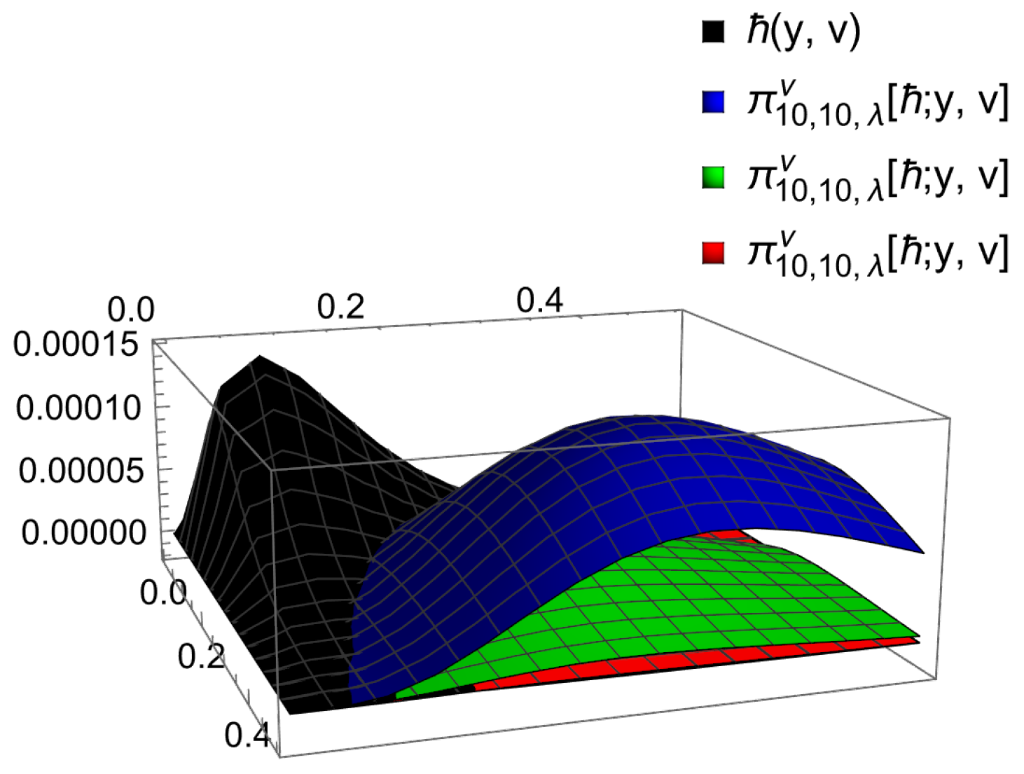
In this section we inspect different values of parameters and through the table and figure presented in the example below. The operators converge uniformly to the function (Block) for different values of (Blue) (Green), and (Red), which is shown in Figure 5. Moreover, Table 3 shows the approximation error of the proposed operator with the help of a common formula , and see Figure 6.
Figure 5.
converges to .
Table 3.
Error approximation table of the operators to .
Figure 6.
Error approximation .
7. Conclusions
In this study, we explore how well the -Szász generalized Beta operators, based on the generalized beta function, can approximate Lebesgue measurable functions. We focus on several aspects, including how these operators converge to a target function as certain parameters change and how quickly this happens, known as the speed of convergence. To understand their strengths and limitations, we also examine their performance on specific functions, such as polynomials and exponential functions. Furthermore, we assess how effectively the operators work across various functions and values, providing a general idea of their approximation ability. To make the findings more accessible and intuitive, we include graphical representations, showing visual examples of how these operators behave under different conditions. This comprehensive approach clearly shows where these operators excel and where they may face challenges.
Author Contributions
N.R.: Writing—original draft; M.F.: conceptualization—review and editing; M.R.: writing—software. All authors have read and agreed to the published version of the manuscript.
Funding
The APC was funded by the Deanship of Graduate Studies and Scientific Research at Qassim University for financial support (QU-APC-2024).
Data Availability Statement
Data are contained within the article.
Acknowledgments
The researchers would like to thank the Deanship of Graduate Studies and Scientific Research at Qassim University for financial support (QU-APC-2024).
Conflicts of Interest
The authors declare no conflicts of interest.
Correction Statement
This article has been republished with a minor correction to the existing affiliation information. This change does not affect the scientific content of the article.
References
- Szász, O. Generalization of S. Bernstein’s polynomials to the infinite interval. Res. Nat. Bur. Stand. 1950, 45, 239–245. [Google Scholar] [CrossRef]
- Bernšteın, S. Demonstration du théoreme de Weierstrass fondée sur le calcul des probabilities. Commum. Soc. Math. Kharkov. 1912, 13, 1–2. [Google Scholar]
- Izadbakhsh, A.; Kalat, A.A.; Khorashadizadeh, S. Observer-based adaptive control for HIV infection therapy using the Baskakov operator. Biomed. Signal Process. Control 2021, 65, 102343. [Google Scholar] [CrossRef]
- Uyan, H.; Aslan, A.O.; Karateke, S.; Buyukyazıcı, I. Interpolation for neural network operators activated with a generalized logistic-type function. J. Inequal. Appl. 2024, 125, 31. [Google Scholar] [CrossRef]
- Zhang, Q.; Mu, M.; Wang, X. A Modified Robotic Manipulator Controller Based on Bernstein-Kantorovich-Stancu Operator. Micromachines 2022, 14, 44. [Google Scholar] [CrossRef] [PubMed]
- Khan, K.; Lobiyal, D.K. Bezier curves based on Lupas (p,q)-analogue of Bernstein functions in CAGD. Comput. Appl. Math. 2017, 317, 458–477. [Google Scholar] [CrossRef]
- Rao, N.; Farid, M.; Ali, R. A Study of Szász–Durremeyer-Type Operators Involving Adjoint Bernoulli Polynomials. Mathematics 2024, 12, 3645. [Google Scholar] [CrossRef]
- Braha, N.L.; Mansour, T.; Mursaleen, M. Some Approximation Properties of Parametric Baskakov–Schurer–Szász Operators Through a Power Series Summability Method. Complex Anal. Oper. Theory 2024, 18, 71. [Google Scholar] [CrossRef]
- Özger, F.; Demiric, K. Approximation by Kantorovich Variant of λ—Schurer Operators and Related Numerical Results. In Topics in Contemporary Mathematics, Analysis and Applications; CRC Press: Boca Raton, FL, USA, 2020; pp. 77–94. [Google Scholar]
- Ansari, K.J.; Özger, F.; Ödemiş, Ö.Z. Numerical and theoretical approximation results for Schurer–Stancu operators with shape parameter λ. Comput. Appl. Math. 2022, 41, 181. [Google Scholar] [CrossRef]
- Khan, A.; Iliyas, M.; Khan, K.; Mursaleen, M. Approximation of conic sections by weighted Lupaş post-quantum Bézier curves. Demonstr. Math. 2022, 55, 328–342. [Google Scholar] [CrossRef]
- Acar, T.; Mursaleen, M.; Mohiuddine, S.A. Stancu type (p, q)-Szász-Mirakyan-Baskakov operators. Commun. Fac. Sci. Univ. Ank. Ser. Math. Stat. 2018, 67, 116–128. [Google Scholar]
- Alotaibi, A. Approximation of GBS type q-Jakimovski-Leviatan-Beta integral operators in Bögel space. Mathematics 2022, 10, 675. [Google Scholar] [CrossRef]
- Mohiuddine, S.A.; Singh, K.K.; Alotaibi, A. On the order of approximation by modified summation-integral-type operators based on two parameters. Demonstr. Math. 2023, 8, 20220182. [Google Scholar] [CrossRef]
- Nasiruzzaman, M.; Rao, N.; Kumar, M.; Kumar, R. Approximation on bivariate parametric extension of Baskakov-Durrmeyer-opeator. Filomat 2021, 35, 2783–2800. [Google Scholar] [CrossRef]
- Çiçek, H.; İzgi, A. Approximation by modified bivariate Bernstein-Durrmeyer and GBS bivariate Bernstein-Durrmeyer operators on a triangular region. Fund. J. Math. Appl. 2022, 5, 135–144. [Google Scholar] [CrossRef]
- Cai, Q.-B.; Aslan, R.; Özger, F.; Srivastava, H.M. Approximation by a new Stancu variant of generalized (λ, μ)-Bernstein operators. Alex. Eng. J. 2024, 107, 205–214. [Google Scholar] [CrossRef]
- Aslan, R. Rate of approximation of blending type modified univariate and bivariate λ-Schurer-Kantorovich operators. Kuwait J. Sci. 2024, 51, 100168. [Google Scholar] [CrossRef]
- Rao, N.; Ayman-Mursaleen, M.; Aslan, R. A note on a general sequence of λ-Szász Kantorovich type operators. Comput. Appl. Math. 2024, 43, 428. [Google Scholar] [CrossRef]
- Izgi, A.; Serenbay, S.K. Approximation by complex Chlodowsky-Szász-Durrmeyer operators in compact disks. Creat. Math. Inform. 2020, 29, 37–44. [Google Scholar] [CrossRef]
- Qi, Q.; Guo, D.; Yang, G. Approximation properties of λ-Szász-Mirakian operators. Int. J. Eng. Res. 2019, 12, 662–669. [Google Scholar]
- Păltănea, R. A class of Durrmeyer type operators preserving linear functions. Ann. Tiberiu Popoviciu Sem. Funct. Equat. Approxim. Convex. 2007, 5, 109–117. [Google Scholar]
- Rao, N.; Raiz, M.; Mursaleen, M.A.; Mishra, V.N. Approximation properties of Generalized beta-type Szász–Mirakjan operators. Iran. J. Sci. 2023, 47, 1771–1781. [Google Scholar] [CrossRef]
- DeVore, R.A.; Lorentz, G.G. Constructive Approximation. In Grundlehren der Mathematischen Wissenschaften; Springer: Berlin/Heidelberg, Germany, 1993; p. 303. [Google Scholar]
- Altomare, F.; Campiti, M. Korovkin-Type Approximation Theory and Its Applications; Appendix A by Michael Pannenberg and Appendix B by Ferdinand Beckhoff; de Gruyter Studies in Mathematics; Walter de Gruyter and Co.: Berlin, Germany, 1994. [Google Scholar]
- Özarslan, M.A.; Aktuglu, H. Local approximation for certain King type operators. Filomat 2013, 27, 173–181. [Google Scholar] [CrossRef]
- Lenze, B. On Lipschitz type maximal functions and their smoothness spaces. Nederl. Akad. Indag. Math. 1988, 50, 53–63. [Google Scholar] [CrossRef]
- Volkov, V.I. On the convergence of sequences of linear positive operators in the space of continuous functions of two variables. Dokl. Akad. Nauk SSSR (NS) 1957, 115, 17–19. (In Russian) [Google Scholar]
- Stancu, F. Apoximarea Funcțiilor de Două și mai Multe Variabile Prin Șiruri de Operatori Liniari și Pozitivi. Ph.D. Thesis, Cluj-Napoca, Romania, 1984. (In Romanian). [Google Scholar]

Disclaimer/Publisher’s Note: The statements, opinions and data contained in all publications are solely those of the individual author(s) and contributor(s) and not of MDPI and/or the editor(s). MDPI and/or the editor(s) disclaim responsibility for any injury to people or property resulting from any ideas, methods, instructions or products referred to in the content. |
© 2024 by the authors. Licensee MDPI, Basel, Switzerland. This article is an open access article distributed under the terms and conditions of the Creative Commons Attribution (CC BY) license (https://creativecommons.org/licenses/by/4.0/).