Enhancing the Aczel–Alsina Model: Integrating Hesitant Fuzzy Logic with Chi-Square Distance for Complex Decision-Making

Abstract

The paper presents an innovative method for tackling multi-attribute decision-making (MADM) problems within a hesitant fuzzy (HF) framework. Initially, the paper generalizes the Chi-square distance measure to the hesitant fuzzy context, defining the HF generalized Chi-square distance. Following this, the paper introduces the power average (P-A) operator and the power geometric (P-G) operator to refine the weights derived from Shannon entropy, taking into account the inter-attribute support. Leveraging the strengths of Aczel–Alsina operations and the power operation, the paper proposes the hesitant fuzzy Aczel–Alsina power weighted average (HFAAPWA) operator and the hesitant fuzzy Aczel–Alsina power weighted geometric (HFAAPWG) operator. Consequently, a hesitant fuzzy Aczel–Alsina power model is constructed. The applicability of this model is demonstrated through a case study examining the urban impacts of cyclonic storm Amphan, and the model’s superiority is highlighted through comparative analysis.

1. Introduction

In a period of rapid technological and disciplinary development, research and practical application in decision-making problems have remained highly active, showing a trend of sustained growth. MADM has been a hot topic, receiving significant attention. In real life, decision-makers (DMs) must deal with increasingly complex and uncertain decision-making information to ensure more accurate and efficient choices. To effectively address the uncertainty and ambiguity of decision indicators, Zadeh [1] first proposed the concept of the fuzzy set (FS). Given the significant strength of fuzzy sets in processing uncertain information, they have achieved great success in various fields [2,3]. In response to an increasingly diverse and intricate array of challenges, the theoretical framework of fuzzy set theory has undergone continuous refinement. This academic evolution has encompassed the introduction of various extended fuzzy sets, including intuitionistic fuzzy sets (IFSs) [4], Pythagorean fuzzy sets (PFSs) [5] and hesitant fuzzy sets (HFSs) [6] which are crucial for addressing the uncertainties and indecisiveness faced by decision-makers during the evaluative process. Furthermore, the development of more generalized models of fuzzy sets, such as (2,1)-fuzzy sets [7] and (m,n)-fuzzy sets [8], has facilitated a more nuanced articulation of the gradations of membership and non-membership degrees. More specifically, unlike Zadeh’s fuzzy set, Atanassov introduced the IFS, which assigns equal importance to both the MD and the NMD. IFSs require that the sum of the MD and the NMD be less than or equal to 1, whereas in practical problems this restriction may be exceeded. To improve this, Yager and Abbasov further proposed the PFS. Correspondingly, these environments are widely applied to decision-making issues in various fields [9]. In practice, decision-makers often found it difficult to determine the MD of a fuzzy set due to some factors such as time constraints, limited theoretical knowledge, or insufficient data, among other reasons. To address this, Torra proposed the concept of the HFS, where the MD is represented by a set of possible values. Compared with other classical fuzzy sets, hesitant fuzzy sets (HFSs) more accurately reflect the indecisiveness and hesitation psychology of decision-makers in practical problems. Numerous classical decision-making methods have been enhanced by experts to accommodate the HFS environment, including   TOPSIS [10], VIKOR [11], and ELECTRE [12], among others. Meanwhile, in contrast to research on some classical decision-making methods, a greater number of researchers have focused on developing aggregation operations and their applications to diverse decision-making issues. This focus is because aggregation operators effectively facilitate information fusion.

Due to the growing volume and complexity of data in practical problems, the role of aggregation operators as crucial techniques for information fusion had been increasingly emphasized by researchers. Originally, Menger [13] introduced the concept of triangular norms, which was subsequently utilized to propose various aggregation operators. For HFSs, Xia and Xu [14] proposed the HF weighted arithmetic (HFWA) operator and weighted geometric (HFWG) operator, in conjunction with algebraic triangular norms. Zhang [11] put forward the HF power average (HFPA) operator and HF power geometric (HFPG) operator, building upon the power average (P-A) [15] and the power geometric (P-G) operators [16]. Power operators serve as nonlinear weighted average aggregation tools, with weight vectors that adjust based on the input arguments, allowing the aggregated values to support and reinforce one another. Based on Einstein’s operational laws, Yu [17] presented the definitions of the HF Einstein weighted averaging (HFEWA) operator and HF Einstein weighted geometric (HFEWG) operator. Combining the Dombi t-norm and t-conorm operations, He [18] constructed the HF Dombi weighted averaging (HFDWA) operator and HF Dombi weighted geometric (HFDWG) operator. Furthermore, within the context of triangular norm theory, the concept of Aczel-Alsina t-norm and t-conorm operations were introduced by Aczel and Alsina [19]. Characterized by their significant parameter variability, these operations are well suited for application in fuzzy multi-attribute decision-making, a feature that has rapidly drawn the attention of scholars in the field. For instance, Senapati and Chen et al. [20] proposed the hesitant fuzzy Aczel–Alsina (AA) weighted averaging (HFAAWA) operator, the hesitant fuzzy Aczel–Alsina weighted geometric (HFAAWG) operator, and the hesitant fuzzy Aczel–Alsina weighted Bonferroni mean (HFAAWBM) operator. These operators were based on the Aczel–Alsina t-norm and t-conorm, as well as the Bonferroni operator. Notably, the Aczel–Alsina t-norm and t-conorm have also been widely used in the intuitionistic fuzzy set [21], the interval-valued fuzzy set [22], the picture fuzzy  set [23], etc.

In addition, distance measures have been extensively utilized in fuzzy sets (FSs) as an important tool for comparing dissimilarity and correlation between data. Previously, Szmidt and Kacprzyk [24] proposed some methods to measure the distance between IFSs based on the Hamming distance and Euclidean distance. Grzegorzewski [25] proposed the two-dimensional distance of IFSs using the Hausdorff metric, considering MD and NMD. Xu and Xia [26] proposed the HF normalized Hamming distance, normalized Euclidean distance, and generalized HF normalized distance, as well as the corresponding generalized weighted distance. Perlibakas [27] has proposed the Chi-square distance, considering the symmetry of the distance function. Ren et al. [28] have extended the Chi-square distance to the Single-valued Neutrosophic Set and have introduced the idea of Chi-square similarity of the Single-valued Neutrosophic Set. Based on existing studies, it is readily apparent that the Hamming distance, Euclidean distance, and Hausdorff metric are among the most commonly used metrics for comparing dissimilarity and correlation between data. In contrast, less research has been conducted on the application of the Chi-square distance. However, the Chi-square distance, developed from the Chi-square statistic, not only has a strong statistical foundation but also effectively applies to discrete data. Moreover, it exhibits greater robustness compared with other distances, such as the Euclidean distance. Therefore, generalizing the Chi-square distance to a broader context holds significant research value.

Shannon entropy, a highly classic method for determining weights, quantifies the uncertainty of data information. However, in the decision-making process, decision-makers often balance different criteria to form judgments, implying that performance values under various criteria have a degree of mutual support. The entropy method fails to account for this aspect, thus necessitating the introduction of power operations to describe the interplay among data across different criteria, leading to the derivation of more precise weights. Considering the scarcity of existing research that applies the Chi-square distance to fuzzy environments and extends the advantages of Aczel–Alsina operators to hesitant fuzzy set contexts, this study generalizes the Chi-square distance to develop a hesitant fuzzy Aczel–Alsina power model. This approach offers novel methodologies and insights for multi-attribute decision-making (MADM) within hesitant fuzzy environments. The primary innovations of this paper are as follows:

(1) Developing the Chi-square distance to the HF environment, the HF generalized Chi-square distance and corresponding similarity measure are proposed and utilized to describe the variability and correlation between data.

(2) Based on the HF generalized Chi-square distance carving of data, the objective weights are obtained using the entropy weighting method, and then the weights are adjusted by combining the power operator to finally obtain the optimized weights.

(3) Considering the merits of the Aczel–Alsina operator and power operator, and based on the hesitation fuzzy generalized Chi-square distance, the hesitation fuzzy Aczel–Alsina power aggregation operator is introduced in this paper, in which the attributes are allowed to support and strengthen mutually.

The work in this paper is organized around the following sections. Section 2 initially review some basics, including several common norms and conorms (Section 2.1), HFSs and basic operations on HFSs (Section 2.2 and Section 2.3), power operators (Section 2.4), and the Shannon entropy weighting method (Section 2.5). Section 3 extends the Chi-squared distance to HFSs and proposes the HF generalized Chi-squared distance and its corresponding similarity measure. Section 4 presents the HF Aczel–Alsina power weighted average operator and HF Aczel–Alsina power weighted geometric operator by combining power operators and Aczel–Alsina operations on HFEs. Section 5 constructs the HF Aczel–Alsina power model on the basis of the proposed aggregation operator. Section 6 applies the model to a real case and obtains the target results. Furthermore, ranking results discussion and sensitivity analysis of the corresponding parameters as well as comparison of some existing methods are given. Eventually, Section 7 gives the conclusion and implications with respect to the work of this paper.

2. Preliminaries

To advance this work, some fundamental knowledge is reviewed.

2.1. Several Norms and Conorms

In this subsection, several norms and conorms will be introduced.

Definition 1

([13]). A triangular norm of a binary operation on the unit interval $[0,1]$ is called a t-norm, i.e., a function $T:[0,1]\times [0,1]⟶[0,1]$ satisfying the following four axioms, for ${\xi }_i,{\xi }_j,{\xi }_l\in [0,1]:$

(T₁)

$T({\xi }_i,{\xi }_j)=T({\xi }_j,{\xi }_i)\left(commutativity\right)$;

(T₂)

$T({\xi }_i,{\xi }_j)\le T({\xi }_i,{\xi }_l)ifj\le l\left(monotonicity\right)$;

(T₃)

$T({\xi }_i,T({\xi }_j,{\xi }_l))=T(T({\xi }_i,{\xi }_j),{\xi }_l)\left(associativity\right)$;

(T₄)

$T({\xi }_i,1)={\xi }_i\left(boundarycondition\right)$.

Definition 2

([29]). A triangular conorm of the binary operation S on the unit interval $[0,1]$ is called a t-conorm, which is monotonicity, commutativity, associativity, and 0 as the neutral element, i.e., a function $S:[0,1]\times [0,1]⟶[0,1]$ satisfying the following four axioms, for ${\xi }_i,{\xi }_j,{\xi }_l\in [0,1]:$

(S₁)

$S({\xi }_i,{\xi }_j)=S({\xi }_j,{\xi }_i)\left(commutativity\right)$;

(S₂)

$S({\xi }_i,{\xi }_j)\le S({\xi }_i,{\xi }_l)ifj\le l\left(monotonicity\right)$;

(S₃)

$S({\xi }_i,S({\xi }_j,{\xi }_l))=S(S({\xi }_i,{\xi }_j),{\xi }_l)\left(associativity\right)$;

(S₄)

$S({\xi }_i,0)={\xi }_i\left(boundarycondition\right)$.

Remark 1

([30]). Listed below are the most commonly used pairs of t-norms and t-conorms, respectively, as follows:

$$\begin{array}{cc}\hfill & \left(1\right)T_M({\xi }_i,{\xi }_j)=min\{{\xi }_i,{\xi }_j\}and{S}_M({\xi }_i,{\xi }_j)=max\{{\xi }_i,{\xi }_j\};\hfill \\ \hfill & \left(2\right)T_P({\xi }_i,{\xi }_j)={\xi }_i·{\xi }_{j}and{S}_P({\xi }_i,{\xi }_j)={\xi }_i+{\xi }_j-{\xi }_i·{\xi }_j;\hfill \\ \hfill & \left(3\right)T_L({\xi }_i,{\xi }_j)=max\{{\xi }_i+{\xi }_j-1,0\}and{S}_L({\xi }_i,{\xi }_j)=min\{{\xi }_i+{\xi }_j,1\};\hfill \\ \hfill & \left(4\right)T_D({\xi }_i,{\xi }_j)=\left\{\begin{array}{cc}{\xi }_i,\hfill & if{\xi }_j=1\hfill \\ {\xi }_i,\hfill & if{\xi }_i=1\hfill \\ 0,\hfill & \mathit{otherwise}\hfill \end{array}\right.and{S}_D({\xi }_i,{\xi }_j)=\left\{\begin{array}{cc}{\xi }_i,\hfill & \mathit{if}{\xi }_j=0\hfill \\ {\xi }_j,\hfill & \mathit{if}{\xi }_i=0.\hfill \\ 1,\hfill & \mathit{otherwise}\hfill \end{array}\right.\hfill \end{array}$$

As early as the 1980s, Aczel–Alsina proposed a class of t-norm in the context of functional equations.

Definition 3

([19,31]). The function $T_A^k{({\xi }_i,{\xi }_j)}_{k\in [0,\infty )}$ of AA t-norms are defined as:

$$\begin{array}{c}\hfill T_A^k({\xi }_i,{\xi }_j)=\left\{\begin{array}{cc}{T}_D({\xi }_i,{\xi }_j),\hfill & \mathit{if}k=0\hfill \\ min\{{\xi }_i,{\xi }_j\},\hfill & \mathit{if}k=\infty .\hfill \\ e^{-{({(-ln{\xi }_i)}^k+{(-ln{\xi }_j)}^k)}^{{\displaystyle \frac{1}{k}}}}\hfill & \mathit{otherwise}\hfill \end{array}\right.\end{array}$$

The function $S_A^k{({\xi }_i,{\xi }_j)}_{k\in [0,\infty )}$ of AA t-conorms are defined as:

$$\begin{array}{c}\hfill S_A^k({\xi }_i,{\xi }_j)=\left\{\begin{array}{cc}{S}_D({\xi }_i,{\xi }_j),\hfill & \mathit{if}k=0\hfill \\ max\{{\xi }_i,{\xi }_j\},\hfill & \mathit{if}k=\infty .\hfill \\ 1-e^{-({(-ln(1-{\xi }_i))}^k+{(-ln{(1-{\xi }_j)}^k)}^{{\displaystyle \frac{1}{k}}}},\hfill & \mathit{otherwise}\hfill \end{array}\right.\end{array}$$

The following are some particular cases: $T_A^0=T_D,T_A^1=T_P,T_A^{\infty }=min,S_A^0=S_D,S_A^1=S_P,S_A^{\infty }=max.$ And AA t-norms increase, while AA t-conorms decrease as the input value increases.

2.2. Hesitant Fuzzy Set

Torra [6] and Narukawa [32] introduced the concept of HFSs as one of the extensions of the classical fuzzy set. The membership degree of HFSs is a set of possible values that can more objectively reflect the hesitation of decision-makers than other classical sets. The following is the specific description of the hesitant fuzzy set.

Definition 4

([32]). Let $H=\{{\eta }_1,{\eta }_2,\dots ,{\eta }_n\}$ be a fixed set, an HFS Γ on H is in terms of a function that when applied to H returns a subset of [0, 1], which can be expressed by the mathematical symbol:

$$A=\{<{\eta }_i,h_{\Gamma }\left({\eta }_i\right)>|{\eta }_i\in H\},$$

(1)

where the function $h_{\Gamma }\left({\eta }_i\right)$ is a set of some different values in $[0,1]$, denoting the possible membership degrees of the element ${\eta }_i\in H$ to $\Gamma$. For simplicity, we call $h=h_{\Gamma }\left({\eta }_i\right)$ a hesitant fuzzy  element (HFE).

In addition, Torra defined operations for complement, union, and intersection of the hesitant fuzzy set as follows:

Definition 5

([32]). Let $\Gamma$, ${\Gamma }_1$, and ${\Gamma }_2$ be three arbitrary HFSs, defining the following operations:

(1)

${\Gamma }^c={\bigcup }_{\gamma \in \Gamma }\{1-\gamma \};$

(2)

${\Gamma }_1\bigcup {\Gamma }_2={\bigcup }_{{\gamma }_1\in {\Gamma }_1,{\gamma }_2\in {\Gamma }_2}max\{{\gamma }_1,{\gamma }_2\};$

(3)

${\Gamma }_1\bigcap {\Gamma }_2={\bigcup }_{{\gamma }_1\in {\Gamma }_1,{\gamma }_2\in {\Gamma }_2}min\{{\gamma }_1,{\gamma }_2\}.$

Moreover, Xia and Xu [33] also outlined some operations for HFEs:

Definition 6

([33]). Let h, $h_1$, and $h_2$ be three arbitrary HFEs, and $\lambda >0$, then

(1)

$h^{\lambda }={\bigcup }_{\gamma \in h}\left\{{\gamma }^{\lambda }\right\};$

(2)

$\lambda h={\bigcup }_{\gamma \in h}\{1-{(1-\gamma )}^{\lambda }\};$

(3)

$h_1⨁h_2={\bigcup }_{{\gamma }_1\in h_1,{\gamma }_2\in h_2}\{{\gamma }_1+{\gamma }_2-{\gamma }_1{\gamma }_2\};$

(4)

$h_1⨂h_2={\bigcup }_{{\gamma }_1\in h_1,{\gamma }_2\in h_2}\left\{{\gamma }_1{\gamma }_2\right\}.$

Based on the generalized ordered weighted average operator proposed by Yager [34] and above operations for HFEs, Xia and Xu [33] proposed a series of aggregation operations for HFEs as follows:

Definition 7

([33]). For a set $\Gamma =\{h_1,h_2,\dots ,h_n\}$ composed of HFEs, the hesitant fuzzy weighted average (HFWA) operator and hesitant fuzzy weighted geometric (HFWG) operator are two mappings $H^n\to H$, such that

$$HFWA(h_1,h_2,\dots ,h_n)=\underset{j=1}{\overset{n}{⨁}}\left({\varpi }_j{h}_j\right)=\bigcup _{{\gamma }_1\in h_1,{\gamma }_2\in h_2,\dots ,{\gamma }_n\in h_n}\{1-\prod _{j=1}^n{(1-{\gamma }_j)}^{{\varpi }_j}\},$$

(2)

$$HFWG(h_1,h_2,\dots ,h_n)=\underset{j=1}{\overset{n}{⨂}}\left(h_j^{{\varpi }_j}\right)=\bigcup _{{\gamma }_1\in h_1,{\gamma }_2\in h_2,\dots ,{\gamma }_n\in h_n}\{\prod _{j=1}^n{\gamma }_j^{{\varpi }_j}\},$$

(3)

where $\omega ={({\varpi }_1,{\varpi }_2,\dots ,{\varpi }_n)}^T$ represents the weight vector corresponding to $h_j(j=1,2,...,n)$ and ${\sum }_{j=1}^n{\varpi }_j=1$.

In this paper, $l_{\left(h_{\Delta }\left(\eta \right)\right)}$ is used to represent the length of HFE $h_{\Delta }\left(\eta \right)$, where $\Delta$ represents arbitrary HFSs. The length of different HFEs may be different, and then it is necessary to normalize the length of HFEs when comparing different HFSs. In this regard,   Farhadinia [35] made some studies and put forward specific comparison methods. In order to ensure that the comparison is reasonable, two assumptions are made:

(A₁)

The values in an HFE are arranged in increasing order.

(A₂)

For two HFSs, ${\Gamma }_1$ and ${\Gamma }_2$, $l_{\left(h\right(\eta \left)\right)}=max\{l_{\left(h_{{\Gamma }_1}\left(\eta \right)\right)},l_{\left(h_{{\Gamma }_2}\left(\eta \right)\right)}\}$. If $l_{\left(h_{{\Gamma }_1}\left(\eta \right)\right)}<l_{\left(h_{{\Gamma }_2}\left(\eta \right)\right)}$, it is necessary to extend the length of $h_{{\Gamma }_1}\left(\eta \right)$ to the same length as $h_{{\Gamma }_2}\left(\eta \right)$ by repeating the maximum value in $h_{{\Gamma }_1}\left(x\right)$.

The specific comparison method is defined as follows:

Definition 8

([35]). For a non-empty fixed set $H=\{{\eta }_1,{\eta }_2,\dots ,{\eta }_n\}$, let ${\Gamma }_1$ and ${\Gamma }_2$ be two HFSs on H. Then, two ordering methods for HFSs are as follows:

One is component-wise ordering:

$${\Gamma }_1\le {\Gamma }_2\mathit{if}{h}_{{\Gamma }_1}^{\left(j\right)}\left({\eta }_i\right)\le h_{{\Gamma }_2}^{\left(j\right)}\left({\eta }_i\right),1\le i\le n,1\le j\le l_{\left({\eta }_i\right)}.$$

The other is total ordering:

$${\Gamma }_1⪯{\Gamma }_2\mathit{if}\Im \left({\Gamma }_1\right)\le \Im \left({\Gamma }_1\right),$$

where $h_{\Delta }^{\left(j\right)}\left({\eta }_i\right)$ represents the jth value in $h_{\Delta }\left({\eta }_i\right)$ after ascending processing, and $\Im (·)$ denotes the score function for HFSs [26] as follows.

$$\Im (\Gamma )={\displaystyle \frac{1}{n}}\sum _{i=1}^n({\displaystyle \frac{1}{l_{\left({\eta }_i\right)}}}\sum _{j=1}^{l_{\left({\eta }_i\right)}}{h}_{\Gamma }^{\left(j\right)}\left({\eta }_i\right)).$$

(4)

Obviously, the score value of HFE $h_{\Gamma }\left({\eta }_i\right)$ is:

$$\Im \left(h_{\Gamma }\left({\eta }_i\right)\right)={\displaystyle \frac{1}{l_{\left({\eta }_i\right)}}}\sum _{j=1}^{l_{\left({\eta }_i\right)}}{h}_{\Gamma }^{\left(j\right)}\left({\eta }_i\right).$$

(5)

To further explore the relationship between different HFSs, Farhadinia [35] also proposed the axiomatic definition of distance and similarity for HFSs.

Definition 9

([35]). Let Γ, ${\Gamma }_1$, and ${\Gamma }_2$ be three arbitrary HFSs on H. A mapping $d:HFS\left(H\right)\times HFS\left(H\right)⟶[0,1]$ is an HF distance measure if it possesses the following conditions:

(1)

$0\le d({\Gamma }_1,{\Gamma }_2)\le 1$;

(2)

$d({\Gamma }_1,{\Gamma }_2)=d({\Gamma }_2,{\Gamma }_1)$;

(3)

$\mathit{If}\Gamma =\left\{0\right\}\mathit{or}\Gamma =\left\{1\right\},\mathit{then}d(\Gamma ,{\Gamma }^c)=1$;

(4)

$d({\Gamma }_1,{\Gamma }_2)=0,\mathit{iff}{\Gamma }_1={\Gamma }_2$;

(5)

$\mathit{Assuming}\mathit{that}\Gamma \le {\Gamma }_1\le {\Gamma }_2,\mathit{then}d(\Gamma ,{\Gamma }_2)\ge max\{d(\Gamma ,{\Gamma }_1),d({\Gamma }_1,{\Gamma }_2)\}$.

Definition 10

([35]). Let Γ, ${\Gamma }_1$, and ${\Gamma }_2$ be three arbitrary HFSs on H. A mapping $S:HFS\left(H\right)\times HFS\left(H\right)⟶[0,1]$ is an HF similarity measure if it possesses the following conditions:

(1)

$0\le S({\Gamma }_1,{\Gamma }_2)\le 1$;

(2)

$S({\Gamma }_1,{\Gamma }_2)=S({\Gamma }_2,{\Gamma }_1)$;

(3)

$\mathit{If}\Gamma =\left\{0\right\}\mathit{or}\Gamma =\left\{1\right\},\mathit{then}S(\Gamma ,{\Gamma }^c)=0$;

(4)

$S({\Gamma }_1,{\Gamma }_2)=1,\mathit{iff}{\Gamma }_1={\Gamma }_2$;

(5)

$\mathit{Assuming}\mathit{that}\Gamma \le {\Gamma }_1\le {\Gamma }_2,\mathit{then}S(\Gamma ,{\Gamma }_1)\le min\{S(\Gamma ,{\Gamma }_1),S({\Gamma }_1,{\Gamma }_2)\}$.

2.3. Aczel–Alsina Operations for HFEs

Since Aczel–Alsina operations have strong fuzzy information processing capabilities, Senapati and Chen et al.[20] have defined some basic operations for HFEs with AA operations.

Definition 11

([20]). For three arbitrary HFEs, h, $h_1$, and $h_2$, with $k\ge 1$ and $\lambda >0$, then the AA operations of HFEs are as follows:

(1)

$h^{\lambda }={\bigcup }_{\gamma \in h}\{e^{-{\left(\lambda {(-ln\gamma )}^k\right)}^{{\displaystyle \frac{1}{k}}}}\}$;

(2)

$\lambda h={\bigcup }_{\gamma \in h}\{1-e^{-{\left(\lambda {(-ln(1-\gamma ))}^k\right)}^{{\displaystyle \frac{1}{k}}}}\}$;

(3)

$h_1⨁h_2={\bigcup }_{{\gamma }_1\in h_1,{\gamma }_2\in h_2}\{1-e^{-{({(-ln(1-{\gamma }_1))}^k+{(-ln(1-{\gamma }_2))}^k)}^{{\displaystyle \frac{1}{k}}}}\}$;

(4)

$h_1⨂h_2={\bigcup }_{{\gamma }_1\in h_1,{\gamma }_2\in h_2}\{e^{-{({(-ln{\gamma }_1)}^k+{(-ln{\gamma }_2)}^k)}^{{\displaystyle \frac{1}{k}}}}\}$.

Theorem 1

([20]). Let $h=\{{\gamma }_1,{\gamma }_2,\dots ,{\gamma }_n\}$, $h_1=\{{\gamma }_1^1,{\gamma }_2^1,\dots ,{\gamma }_n^1\}$, and $h_2=\{{\gamma }_1^2,{\gamma }_2^2,\dots ,{\gamma }_n^2\}$ be three HFEs. Then

(1)

$h_1⨁h_2=h_2⨁h_1$;

(2)

$h_1⨂h_2=h_2⨂h_1$;

(3)

$\lambda (h_1⨂h_2)=\lambda h_1⨂\lambda h_2,\lambda >0$;

(4)

$({\lambda }_1+{\lambda }_2)h={\lambda }_{1}h⨁{\lambda }_{2}h,{\lambda }_1,{\lambda }_2>0$;

(5)

${(h_1⨂h_2)}^{\lambda }=h_1^{\lambda }⨂h_2^{\lambda },\lambda >0$;

(6)

$h^{{\lambda }_1}⨂h^{{\lambda }_2}=h^{({\lambda }_1+{\lambda }_2)},{\lambda }_1,{\lambda }_2>0$.

2.4. Power Average (P-A) Operator and Power Geometric (P-G) Operator

Yager [15] proposed the power average (P-A) operator, which allows parameter values to support each other throughout the optimization process. This allows the P-A operator to provide a greater degree of flexibility in data aggregation methods. After that, Xu and Yager [16] proposed the power geometric (P-G) operator based on the P-A operator and geometric mean.

Definition 12

([35]). Let $\zeta =({\zeta }_1,{\zeta }_2,\dots ,{\zeta }_n)$ denote the collection of parameter values, and the P-A operator and the P-G operator are defined as follows:

$$P-A({\zeta }_1,{\zeta }_2,\dots ,{\zeta }_n)={\displaystyle \frac{{\sum }_{i=1}^n(1+T\left({\zeta }_i\right)){\zeta }_i}{{\sum }_{i=1}^n(1+T\left({\zeta }_i\right))}},$$

(6)

$$P-G({\zeta }_1,{\zeta }_2,\dots ,{\zeta }_n)=\prod _{i=1}^n{\left({\zeta }_i\right)}^{{\displaystyle \frac{1+T\left({\zeta }_i\right)}{{\sum }_{i=1}^n(1+T\left({\zeta }_i\right))}}},$$

(7)

where

$$T\left({\zeta }_i\right)=\sum _{j=1,j\ne i}^{n}Sup({\zeta }_i,{\zeta }_j),$$

(8)

where $Sup({\zeta }_i,{\zeta }_j)$ represents the support ${\zeta }_i$ receives from ${\zeta }_j$, and $T\left({\zeta }_i\right)$ represents all the support ${\zeta }_i$ receives from other than itself.

Note that the support function must meet the following characteristics:

$$\begin{array}{cc}\hfill & \left(1\right)Sup({\zeta }_i,{\zeta }_j)\in [0,1];\hfill \\ \hfill & \left(2\right)Sup({\zeta }_i,{\zeta }_j)=Sup({\zeta }_j,{\zeta }_i);\hfill \\ \hfill & \left(3\right)Sup({\zeta }_i,{\zeta }_j)\ge Sup({\zeta }_m,{\zeta }_n),if|{\zeta }_i-{\zeta }_j|<|{\zeta }_m-{\zeta }_n|.\hfill \end{array}$$

Colloquially, the level of support increases with similarity and proximity.

Without loss of generality, the P-A operator and the P-G operator can simply be written as:

$$P-A({\zeta }_1,{\zeta }_2,\dots ,{\zeta }_n)=\sum _{i=1}^n{\omega }_i{\zeta }_i,$$

(9)

$$P-G({\zeta }_1,{\zeta }_2,\dots ,{\zeta }_n)=\prod _{i=1}^n{\left({\zeta }_i\right)}^{{\omega }_i},$$

(10)

where ${\omega }_i={\displaystyle \frac{1+T\left({\zeta }_i\right)}{{\sum }_{i=1}^{n}1+T\left({\zeta }_i\right)}}$. ${\omega }_i$ represents a set of weights, satisfying ${\omega }_i\ge 0$ and ${\sum }_{i=1}^n{\omega }_i=1$. (9) and (10) are the weighted average and weighted geometric with respect to ${\zeta }_i$. In particular, when the support values are equal, both the P-A and P-G operators can be regarded as simple means. Such as $Sup({\zeta }_i,{\zeta }_j)=0$, the P-A operator and the P-G operator are denoted as:

$$P-A({\zeta }_1,{\zeta }_2,\dots ,{\zeta }_n)={\displaystyle \frac{1}{n}}\sum _{i=1}^n{\zeta }_i,$$

(11)

$$P-G({\zeta }_1,{\zeta }_2,\dots ,{\zeta }_n)={\left(\prod _{i=1}^n{\zeta }_i\right)}^{{\displaystyle \frac{1}{n}}}.$$

(12)

Furthermore, it must be noted that both the P-A operator and P-G operator have commutativity, boundedness, and idempotence, but they do not have monotonicity for an arbitrary input value.

2.5. Shannon Entropy Weight

The concept of entropy first appeared in thermodynamics to describe irreversible phenomena in motion. When Shannon [36] studied the measurement of uncertainty in random variables, he found that their mathematical form was identical to thermal entropy. Therefore, Shannon referred to it as entropy, commonly known as information entropy or Shannon entropy. The introduction of information entropy greatly optimizes the decision-making process because it can quantify the differences between data sets, effectively deal with the uncertainty of the data, and tell the decision-maker that the amount of information is exactly equal to the entropy of the random variable. The procedure is as follows [37]:

Let $R={\left[r_{ij}\right]}_{n\times m}$ be a decision matrix, and $r_{ij}$ indicates the value of the ith alternative under the jth attribute.

Step 1. Normalizing the element $r_{ij}$ in the decision matrix using the following formula as $e_{ij}$:

$$e_{ij}={\displaystyle \frac{r_{ij}}{{\sum }_{i=1}^n{r}_{ij}}},$$

(13)

Step 2. Calculating the information entropy of the jth attribute using the following formula:

$$E_j=-y\sum _{i=1}^n{e}_{ij}ln{e}_{ij},$$

(14)

where $y={\displaystyle \frac{1}{lnn}}$ represents the entropy constant, and $e_{ij}ln{e}_{ij}=0$ if $e_{ij}=0$.

Step 3. Calculating the weight vector $W=(w_1,w_2,\dots ,w_m)$ as follows:

$$w_j={\displaystyle \frac{1-E_j}{{\sum }_{i=1}^m(1-E_j)}}.$$

(15)

3. HF Generalized Chi-Square Distance

The Chi-square distance is generated from the Pearson Chi-square test statistic   ${\chi }^2={\sum }_{i=1}^n{\displaystyle \frac{{(O_i-E_i)}^2}{E_i}}$, which is used to assess the difference between the observed frequency, $O_i$, and the expected frequency, $E_i$. On this basis, the Chi-square statistic is developed as a distance metric by considering the symmetry of distance function. Then Chi-square distance between vectors $O=(o_1,o_2,\dots ,o_n)$ and $E=(e_1,e_2,\dots ,e_n)$ is as follows [27]:

$$d(O,E)=\sum _{i=1}^n{\displaystyle \frac{{(o_i-e_i)}^2}{o_i+e_i}}.$$

The Chi-square distance has been successfully used as an important distance measure in many fields, such as face recognition, picture processing, etc [27,38,39]. Based on these, a new HF generalized Chi-square distance is defined in this paper.

Definition 13.

Given a non-empty finite set $H=\{{\eta }_1,{\eta }_2,\dots ,{\eta }_n\}$, $A=\{<{\eta }_i,u_A\left({\eta }_i\right)>|{\eta }_i\in H\}$ and $B=\{<{\eta }_i,u_B\left({\eta }_i\right)>|{\eta }_i\in H\}$ are two HFSs on H. Hypothesis, for each ${\eta }_i\in H$, the length of $u_A\left({\eta }_i\right)$ is the same as $u_B\left({\eta }_i\right)$, i.e., $l=l\left(u_A\left({\eta }_i\right)\right)=l\left(u_B\left({\eta }_i\right)\right)$. For ${\eta }_i$, the distance between $u_A\left({\eta }_i\right)$ and $u_B\left({\eta }_i\right)$ is defined as follows:

$$d(u_A\left({\eta }_i\right),u_B\left({\eta }_i\right))={\displaystyle \frac{2}{l}}\sum _{j=1}^l{\displaystyle \frac{|u_A^{\left(j\right)}\left({\eta }_i\right)-u_B^{\left(j\right)}\left({\eta }_i\right){|}^p}{1+u_A^{\left(j\right)}\left({\eta }_i\right)+u_B^{\left(j\right)}\left({\eta }_i\right)}},$$

(16)

where $u_{*}^{\left(j\right)}\left({\eta }_i\right)$ is the jth largest value in $u_{*}\left({\eta }_i\right)$ (∗ is A or B), and $p\ge 1$. For HFSs A and B, the distance between A and B is defined:

$$d(A,B)={\displaystyle \frac{2}{nl}}\sum _{i=1}^n\sum _{j=1}^l{\displaystyle \frac{|u_A^{\left(j\right)}\left({\eta }_i\right)-u_B^{\left(j\right)}\left({\eta }_i\right){|}^p}{1+u_A^{\left(j\right)}\left({\eta }_i\right)+u_B^{\left(j\right)}\left({\eta }_i\right)}}.$$

(17)

To prove that the HF generalized Chi-square distance is a valid distance measure, that is, it satisfies several axiomatic properties of Definition 9, we need the following lemma.

Lemma 1.

Suppose $e,f,g$ are three nonnegative real numbers satisfying $0\le e\le f\le g$. Let ϑ and p both be positive real numbers and $p\ge 1$. Then

$${\displaystyle \frac{{|e-g|}^p}{\vartheta +e+g}}\ge max\{{\displaystyle \frac{{|e-f|}^p}{\vartheta +e+f}},{\displaystyle \frac{{|f-g|}^p}{\vartheta +f+g}}\}.$$

Proof. 

First prove ${\displaystyle \frac{{|e-g|}^p}{\vartheta +e+g}}\ge {\displaystyle \frac{{|e-f|}^p}{\vartheta +e+f}}$. Assuming $f\left(x\right)={\displaystyle \frac{{|e-x|}^p}{\vartheta +e+x}}$, and $x\ge e$. Taking the derivative of $f\left(x\right)$ with respect to x yields:

$$f^{\prime }\left(x\right)={\displaystyle \frac{p(\vartheta +e+x){(x-e)}^{p-1}-{(x-e)}^p}{{(\vartheta +e+x)}^2}}.$$

Since the range of values of p and $x\ge e$, it is easy to know $f^{\prime }\left(x\right)\ge 0$. Then $f\left(x\right)$ increases monotonically with respect to x, and it is proven that ${\displaystyle \frac{{|e-g|}^p}{\vartheta +e+g}}\ge {\displaystyle \frac{{|e-f|}^p}{\vartheta +e+f}}$.

In the same way to certificate ${\displaystyle \frac{{|e-g|}^p}{\vartheta +e+g}}\ge {\displaystyle \frac{{|f-g|}^p}{\vartheta +f+g}}$. Similarly, assuming $g\left(x\right)={\displaystyle \frac{{|g-x|}^p}{\vartheta +g+x}}$. The derivative of $g\left(x\right)$ with respect to x is:

$$g^{\prime }\left(x\right)={\displaystyle \frac{-p(\vartheta +g+x){(g-x)}^{p-1}-{(g-x)}^p}{{(\vartheta +g+x)}^2}}.$$

Because $p\ge 1$ and $x\le g$, it is easy to know that $g^{\prime }\left(x\right)\le 0$. Then $g\left(x\right)$ decreases monotonically with respect to x, and it is proven that ${\displaystyle \frac{{|e-g|}^p}{\vartheta +e+g}}\ge {\displaystyle \frac{{|f-g|}^p}{\vartheta +f+g}}$. Therefore, ${\displaystyle \frac{{|e-g|}^p}{\vartheta +e+g}}\ge max\{{\displaystyle \frac{{|e-f|}^p}{\vartheta +e+f}},{\displaystyle \frac{{|f-g|}^p}{\vartheta +f+g}}\}$.    □

Theorem 2.

The distance measure $d(A,B)$ satisfies the axiomatic properties of Definition 9.

Proof. 

(1) Known $u_A^{\left(j\right)}\left({\eta }_i\right),u_B^{\left(j\right)}\left({\eta }_i\right)\in [0,1]$. Obviously $d(A,B)\ge 0$, so we just need to prove $d(A,B)\le 1$. For Equation (17), if $0\le u_B^{\left(j\right)}\left({\eta }_i\right)\le u_A^{\left(j\right)}\left({\eta }_i\right)\le 1$, we have:

$$\begin{array}{cc}\hfill {\displaystyle \frac{|u_A^{\left(j\right)}\left({\eta }_i\right)-u_B^{\left(j\right)}\left({\eta }_i\right){|}^p}{1+u_A^{\left(j\right)}\left({\eta }_i\right)+u_B^{\left(j\right)}\left({\eta }_i\right)}}& ={\displaystyle \frac{u_A^{\left(j\right)}\left({\eta }_i\right)-u_B^{\left(j\right)}\left({\eta }_i\right)}{1+u_A^{\left(j\right)}\left({\eta }_i\right)+u_B^{\left(j\right)}\left({\eta }_i\right)}}{(u_A^{\left(j\right)}\left({\eta }_i\right)-u_B^{\left(j\right)}\left({\eta }_i\right))}^{p-1}\hfill \\ \hfill & \le {\displaystyle \frac{u_A^{\left(j\right)}\left({\eta }_i\right)-u_B^{\left(j\right)}\left({\eta }_i\right)}{1+u_A^{\left(j\right)}\left({\eta }_i\right)+u_B^{\left(j\right)}\left({\eta }_i\right)}}\le {\displaystyle \frac{u_A^{\left(j\right)}\left({\eta }_i\right)}{u_A^{\left(j\right)}\left({\eta }_i\right)+u_A^{\left(j\right)}\left({\eta }_i\right)}}={\displaystyle \frac{1}{2}}.\hfill \end{array}$$

Uniformly, if $0\le u_A^{\left(j\right)}\left({\eta }_i\right)\le u_B^{\left(j\right)}\left({\eta }_i\right)\le 1$, we equally obtain ${\displaystyle \frac{|u_A^{\left(j\right)}\left({\eta }_i\right)-u_B^{\left(j\right)}\left({\eta }_i\right){|}^p}{1+u_A^{\left(j\right)}\left({\eta }_i\right)+u_B^{\left(j\right)}\left({\eta }_i\right)}}\le {\displaystyle \frac{1}{2}}$. Therefore, it is easy to obtain:

$$d(A,B)={\displaystyle \frac{2}{nl}}\sum _{i=1}^n\sum _{j=1}^l{\displaystyle \frac{|u_A^{\left(j\right)}\left({\eta }_i\right)-u_B^{\left(j\right)}\left({\eta }_i\right){|}^p}{1+u_A^{\left(j\right)}\left({\eta }_i\right)+u_B^{\left(j\right)}\left({\eta }_i\right)}}\le 1.$$

Hence $0\le d(A,B)\le 1$ is satisfied;

(2)

$$\begin{array}{cc}\hfill d(A,B)& ={\displaystyle \frac{2}{nl}}\sum _{i=1}^n\sum _{j=1}^l{\displaystyle \frac{|u_A^{\left(j\right)}\left({\eta }_i\right)-u_B^{\left(j\right)}\left({\eta }_i\right){|}^p}{1+u_A^{\left(j\right)}\left({\eta }_i\right)+u_B^{\left(j\right)}\left({\eta }_i\right)}}\hfill \\ \hfill & ={\displaystyle \frac{2}{nl}}\sum _{i=1}^n\sum _{j=1}^l{\displaystyle \frac{|u_B^{\left(j\right)}\left({\eta }_i\right)-u_A^{\left(j\right)}\left({\eta }_i\right){|}^p}{1+u_A^{\left(j\right)}\left({\eta }_i\right)+u_B^{\left(j\right)}\left({\eta }_i\right)}}=d(B,A),\hfill \end{array}$$

that is, $d(A,B)=d(B,A)$;

(3) Let $A=\left\{1\right\}$, then $A^c=\left\{0\right\}$, i.e., for arbitrary ${\eta }_i\in H$, $u_A^{\left(j\right)}\left({\eta }_i\right)=\left\{1\right\},u_{A^c}^{\left(j\right)}\left({\eta }_i\right)=\left\{0\right\}$. Apparently, $d(A,A^c)={\displaystyle \frac{2}{nl}}{\sum }_{i=1}^n{\sum }_{t=1}^l{\displaystyle \frac{|u_A^{\left(j\right)}\left({\eta }_i\right)-u_{A_c}^{\left(j\right)}\left({\eta }_i\right){|}^p}{1+u_A^{\left(j\right)}\left({\eta }_i\right)+u_{A_c}^{\left(j\right)}\left({\eta }_i\right)}}=1$. Analogously, when $A=\left\{0\right\}$, i.e., $A^c=\left\{1\right\}$, then $d(A,A^c)=1$;

(4) When $A=B$, i.e., for each ${\eta }_i\in H$, $u_A^{\left(j\right)}\left({\eta }_i\right)=u_A^{\left(j\right)}\left({\eta }_i\right)$, that is, $d(A,B)=0$;

(5) By Definition 8, if $A\le B\le C$, i.e., for each ${\eta }_i\in H$, $0\le u_A^{\left(j\right)}\left({\eta }_i\right)\le u_B^{\left(j\right)}\left({\eta }_i\right)\le u_C^{\left(j\right)}\left({\eta }_i\right)\le 1$. From Lemma 1, let $\vartheta =1$, we can obtain

$${\displaystyle \frac{|u_A^{\left(j\right)}\left({\eta }_i\right)-u_C^{\left(j\right)}\left({\eta }_i\right){|}^p}{1+u_A^{\left(j\right)}\left({\eta }_i\right)+u_C^{\left(j\right)}\left({\eta }_i\right)}}\ge max\{{\displaystyle \frac{|u_A^{\left(j\right)}\left({\eta }_i\right)-u_B^{\left(j\right)}\left({\eta }_i\right){|}^p}{1+u_A^{\left(j\right)}\left({\eta }_i\right)+u_B^{\left(j\right)}\left({\eta }_i\right)}},{\displaystyle \frac{|u_B^{\left(j\right)}\left({\eta }_i\right)-u_C^{\left(j\right)}\left({\eta }_i\right){|}^p}{1+u_B^{\left(j\right)}\left({\eta }_i\right)+u_C^{\left(j\right)}\left({\eta }_i\right)}}\}.$$

By Equation (17), it is not hard to know $d(A,C)\ge max\left\{d\right(A,B),d(B,C\left)\right\}$. Therefore, the proof that $d(A,B)$ is a valid distance measure of the HFSs A and B is completed. Then, for the given $A=\{<{\eta }_i,u_A\left({\eta }_i\right)>|{\eta }_i\in H\}$ and $B=\{<{\eta }_i,u_B\left({\eta }_i\right)>|{\eta }_i\in H\}$, a new similarity measure based on the HF generalized Chi-square distance is proposed.    □

Definition 14.

For a non-empty finite set $H=\{{\eta }_1,{\eta }_2,\cdots ,{\eta }_n\}$, $A=\{<{\eta }_i,u_A\left({\eta }_i\right)>|{\eta }_i\in H\}$ and $B=\{<{\eta }_i,u_B\left({\eta }_i\right)>|{\eta }_i\in H\}$ are two HFSs on H. Hypothesis, for each ${\eta }_i\in H$, the length of $u_A\left({\eta }_i\right)$ is the same as $u_B\left({\eta }_i\right)$, i.e., $l=l\left(u_A\left({\eta }_i\right)\right)=l\left(u_B\left({\eta }_i\right)\right)$. For ${\eta }_i$, the similarity measure between $u_A\left({\eta }_i\right)$ and $u_B\left({\eta }_i\right)$ is defined as follows:

$$S(u_A\left({\eta }_i\right),u_B\left({\eta }_i\right))=1-{\displaystyle \frac{2}{l}}\sum _{j=1}^l{\displaystyle \frac{|u_A^{\left(j\right)}\left({\eta }_i\right)-u_B^{\left(j\right)}\left({\eta }_i\right){|}^p}{1+u_A^{\left(j\right)}\left({\eta }_i\right)+u_B^{\left(j\right)}\left({\eta }_i\right)}},$$

(18)

where $u_{*}^{\left(j\right)}\left({\eta }_i\right)$ means that the jth largest value in $u_{*}\left({\eta }_i\right)$ (∗ is A or B), and $p\ge 1$. For HFSs A and B, the similarity measure between A and B is:

$$S(A,B)=1-{\displaystyle \frac{2}{nl}}\sum _{i=1}^n\sum _{j=1}^l{\displaystyle \frac{|u_A^{\left(j\right)}\left({\eta }_i\right)-u_B^{\left(j\right)}\left({\eta }_i\right){|}^p}{1+u_A^{\left(j\right)}\left({\eta }_i\right)+u_B^{\left(j\right)}\left({\eta }_i\right)}},$$

(19)

Theorem 3.

The similarity measure $S(A,B)$ satisfies the axiomatic properties of Definition 10.

Proof. 

The proof process is similar to that of Theorem 2.    □

4. HF Aczel–Alsina Power Weighted Operators

Based on the power operations and Aczel–Alsina operations for HFEs, the HF Aczel–Alsina power weighted average (HFAAPWA) operator and HF Aczel–Alsina power weighted geometric (HFAAPWG) operator are proposed.

4.1. HF Aczel–Alsina Power Weighted Average Operator

In this section, we propose the HF Aczel–Alsina power weighted average (HFAAPWA) operator by combining of Aczel–Alsina operations and power operations on HFEs.

Definition 15.

Let $U=\left\{u_i\right|i=1,2,\cdots ,n\}$ be an HFS, and $\beta ={({\beta }_1,{\beta }_2,\cdots ,{\beta }_n)}^T$ is the weight vector of $u_i(i=1,2,\cdots ,n)$, with ${\beta }_i>0$ and ${\sum }_{i=1}^n{\beta }_i=1$. Then the HFAAPWA operator is   as follows:

$$\begin{array}{cc}\hfill HFAAPWA(u_1,u_2,\cdots ,u_n)& ={\displaystyle \frac{{⨁}_{i=1}^n{\beta }_i(1+T\left(u_i\right))u_i}{{\sum }_{i=1}^n{\beta }_i(1+T\left(u_i\right))}}\hfill \\ \hfill & ={\displaystyle \frac{\left({\beta }_1(1+T\left(u_1\right))u_1\right)⨁\left({\beta }_2(1+T\left(u_2\right))u_2\right)⨁···⨁\left({\beta }_n(1+T\left(u_n\right))u_n\right)}{{\sum }_{i=1}^n{\beta }_i(1+T\left(u_i\right))}}.\hfill \end{array}$$

Theorem 4.

The HFAAPWA operator aggregation still yields an HFE.

$$\begin{array}{cc}\hfill \mathit{HFAAPWA}(u_1,u_2,\cdots ,u_n)& ={\displaystyle \frac{{⨁}_{i=1}^n{\beta }_i(1+T\left(u_i\right))u_i}{{\sum }_{i=1}^n{\beta }_i(1+T\left(u_i\right))}}\hfill \\ \hfill & =\bigcup _{{\gamma }_1\in u_1,{\gamma }_2\in u_2,\cdots ,{\gamma }_n\in u_n}\{1-e^{-{({\sum }_{1=1}^n{\displaystyle \frac{{\beta }_i(1+T\left(u_i\right))}{{\sum }_{i=1}^n{\beta }_i(1+T\left(u_i\right))}}{(-ln(1-{\gamma }_i))}^k)}^{{\displaystyle \frac{1}{k}}}}\}.\hfill \end{array}$$

(20)

Proof. 

The proof of Theorem 4 is given by mathematical induction:

when $n=2$,

$$\begin{array}{cc}\hfill HFAAPWA(u_1,u_2)& ={\displaystyle \frac{{\beta }_1(1+T\left(u_1\right))u_1⨁{\beta }_2(1+T\left(u_2\right))u_2}{{\sum }_{i=1}^2{\beta }_i(1+T\left(u_i\right))}}\hfill \\ \hfill & =\bigcup _{{\gamma }_1\in u_1,{\gamma }_2\in u_2}\{1-e^{-{({\displaystyle \frac{({\beta }_1(1+T\left(u_1\right)){(-ln(1-{\gamma }_1))}^k+{\beta }_2(1+T\left(u_2\right)){(-ln(1-{\gamma }_2))}^k)}{{\beta }_1(1+T\left(u_1\right))+{\beta }_2(1+T\left(u_2\right))}})}^{{\displaystyle \frac{1}{k}}}}\}.\hfill \end{array}$$

Hence, Equation (20) is correct for $n=2$.

Then, assuming $n=t$, we can obtain

$$\begin{array}{cc}\hfill HFAAPWA(u_1,u_2,\cdots ,u_t)& ={\displaystyle \frac{{⨁}_{i=1}^t{\beta }_i(1+T\left(u_i\right))u_i}{{\sum }_{i=1}^t{\beta }_i(1+T\left(u_i\right))}}\hfill \\ \hfill & =\bigcup _{{\gamma }_1\in u_1,{\gamma }_2\in u_2,\cdots ,{\gamma }_t\in u_n}\{1-e^{-{({\sum }_{i=1}^t{\displaystyle \frac{{\beta }_i(1+T\left(u_i\right))}{{\sum }_{i=1}^t{\beta }_i(1+T\left(u_i\right))}}{(-ln(1-{\gamma }_i))}^k)}^{{\displaystyle \frac{1}{k}}}}\}.\hfill \end{array}$$

Now, for $n=t+1$,

$$\begin{array}{cc}\hfill HFAAPWA(u_1,u_2,\cdots ,u_t,u_{t+1})& ={\displaystyle \frac{{⨁}_{i=1}^{t+1}{\beta }_i(1+T\left(u_i\right))u_i}{{\sum }_{i=1}^t{\beta }_i(1+T\left(u_i\right))}}\hfill \\ \hfill & =\bigcup _{{\gamma }_1\in u_1,{\gamma }_2\in u_2,\cdots ,{\gamma }_t\in u_t}\{1-e^{-{({\sum }_{1=1}^t{\displaystyle \frac{{\beta }_i(1+T\left(u_i\right))}{{\sum }_{i=1}^t{\beta }_i(1+T\left(u_i\right))}}{(-ln(1-{\gamma }_i))}^k)}^{{\displaystyle \frac{1}{k}}}}\}\hfill \\ \hfill & ⨁\bigcup _{{\gamma }_{t+1}\in u_{t+1}}\{1-e^{-{({\displaystyle \frac{{\beta }_{t+1}(1+T\left(u_{t+1}\right)){(-ln(1-{\gamma }_{t+1}))}^k}{{\beta }_{t+1}(1+T\left(u_{t+1}\right))}})}^{{\displaystyle \frac{1}{k}}}}\}\hfill \\ \hfill & =\bigcup _{{\gamma }_1\in u_1,{\gamma }_2\in u_2,\cdots ,{\gamma }_{t+1}\in u_{t+1}}\{1-e^{-{({\sum }_{1=1}^{t+1}{\displaystyle \frac{{\beta }_i(1+T\left(u_i\right))}{{\sum }_{i=1}^{t+1}{\beta }_i(1+T\left(u_i\right))}}{(-ln(1-{\gamma }_i))}^k)}^{{\displaystyle \frac{1}{k}}}}\}.\hfill \end{array}$$

Therefore, Equation (20) is correct for $n=t+1$. It is proved that Equation (20) is valid for any n.    □

4.2. HF Aczel–Alsina Power Weighted Geometric Operator

Along the same thought, based on Aczel–Alsina operations and power operations applied to HFEs, the HF Aczel–Alsina power weighted geometric (HFAAPWG) operator   is defined.

Definition 16.

Let $U=\left\{u_i\right|i=1,2,\cdots ,n\}$ be an HFS, and $\beta ={({\beta }_1,{\beta }_2,\cdots ,{\beta }_n)}^T$ is the weight vector of $u_i(i=1,2,\cdots ,n)$, with ${\beta }_i>0$ and ${\sum }_{i=1}^n{\beta }_i=1$. Then the HFAAPWG operator is   as follows:

$$\begin{array}{cc}\hfill HFAAPWG(u_1,u_2,\cdots ,u_n)& =\underset{i=1}{\overset{n}{⨂}}{\left(u_i\right)}^{{\displaystyle \frac{{\beta }_i(1+T\left(u_i\right))}{{\sum }_{i=1}^n{\beta }_i(1+T\left(u_i\right))}}}\hfill \\ \hfill & ={\left(u_1\right)}^{{\displaystyle \frac{{\beta }_1(1+T\left(u_1\right))}{{\sum }_{i=1}^n{\beta }_i(1+T\left(u_i\right))}}}⨂{\left(u_2\right)}^{{\displaystyle \frac{{\beta }_2(1+T\left(u_2\right))}{{\sum }_{i=1}^n{\beta }_i(1+T\left(u_i\right))}}}⨂···⨂{\left(u_n\right)}^{{\displaystyle \frac{{\beta }_n(1+T\left(u_n\right))}{{\sum }_{i=1}^n{\beta }_i(1+T\left(u_i\right))}}}.\hfill \end{array}$$

Theorem 5.

The HFAAPWG operator aggregation still yields an HFE.

$$\begin{array}{cc}\hfill HFAAPWG(u_1,u_2,\cdots ,u_n)& ={\displaystyle \frac{{⨁}_{i=1}^n{\beta }_i(1+T\left(u_i\right))u_i}{{\sum }_{i=1}^n{\beta }_i(1+T\left(u_i\right))}}\hfill \\ \hfill & =\bigcup _{{\gamma }_1\in u_1,{\gamma }_2\in u_2,\cdots ,{\gamma }_n\in u_n}\{e^{-{({\sum }_{i=1}^n{\displaystyle \frac{{\beta }_i(1+T\left(u_i\right))}{{\sum }_{i=1}^n{\beta }_i(1+T\left(u_i\right))}}{(-ln{\gamma }_i)}^k)}^{{\displaystyle \frac{1}{k}}}}\}.\hfill \end{array}$$

(21)

Proof. 

The proof process is similar to that of Theorem 4.    □

5. Hesitant Fuzzy Power Aczel–Alsina Model

Regarding a MADM matter, consider multiple attributes $C=\{C_1,C_2,\cdots ,C_n\}$, and $A=\{A_1,A_2,\cdots ,A_m\}$ as a set of alternatives, and $\beta ={({\beta }_1,{\beta }_2,\cdots ,{\beta }_n)}^T$ corresponds to the weight of each attribute, with ${\beta }_i>0$ and ${\sum }_{i=1}^n{\beta }_i=1$. Let DMs provide the HF decision matrix $R={\left(u_{\varphi \phi }\right)}_{m\times n}$, where HFE $u_{\varphi \phi }=\left\{u_{\varphi \phi }^{\left(j\right)}\right|j=1,2,\cdots ,l\left(u_{\varphi \phi }\right)\}$ represents the evaluation value of alternative $A_{\varphi }$ under attribute $C_{\phi }$, and each HFE has the same length, i.e., $l\left(u_{\varphi \phi }\right)=l$. Supplementarily, $u_{\varphi \phi }^{\left(j\right)}$ means the jth largest value in $u_{\varphi \phi }$, with $u_{\varphi \phi }^{\left(j\right)}\in [0,1]$. Consequently, the HF decision matrix, R, is represented by Equation (22) as follows:

$$\begin{array}{cc}\hfill \mathbf{R}=& {\left(u_{\varphi \phi }\right)}_{m\times n}\hfill \\ \hfill =& \left(\begin{array}{cccc}{u}_{11}& u_{12}& \cdots & u_{1n}\\ u_{21}& u_{22}& \cdots & u_{2n}\\ ⋮& ⋮& \ddots & ⋮\\ u_{m1}& u_{m2}& \cdots & u_{mn}\end{array}\right),\hfill \end{array}$$

(22)

where each of $u_{\varphi \phi }$ is an HFE. The following are the detailed steps of the HF Aczel–Alsina power model.

Step 1. Considering the nature of attributes, the HF decision matrix $R={\left(u_{\varphi \phi }\right)}_{m\times n}$ is transformed into a normalization decision matrix $\Re =\left({\mu }_{\varphi \phi }\right)$.

$$\begin{array}{c}\hfill {\mu }_{\varphi \phi }=\left\{\begin{array}{cc}{u}_{\varphi \phi },\hfill & \mathrm{for}\mathrm{beneficial}\mathrm{attribute}{C}_{\phi };\hfill \\ {\left(u_{\varphi \phi }\right)}^c,\hfill & \mathrm{for}\cos \mathrm{t}\mathrm{attribute}{C}_{\phi }.\hfill \end{array}\right.\end{array}$$

(23)

Therefore, the normalized matrix can be obtained.

$$\begin{array}{cc}\hfill \Re =& {\left({\mu }_{\varphi \phi }\right)}_{m\times n}\hfill \\ \hfill =& \left(\begin{array}{cccc}{\mu }_{11}& {\mu }_{12}& \cdots & {\mu }_{1n}\\ {\mu }_{21}& {\mu }_{22}& \cdots & {\mu }_{2n}\\ ⋮& ⋮& \ddots & ⋮\\ {\mu }_{m1}& {\mu }_{m2}& \cdots & {\mu }_{mn}\end{array}\right).\hfill \end{array}$$

(24)

Step 2. Calculating the generalized Chi-square distance for each ${\mu }_{\varphi \phi }$ to ${\mu }^{+}$ and ${\mu }^{-}$ by Equation (16). Then, calculating the remoteness index, $I_{\varphi \phi }$, for each ${\mu }_{\varphi \phi }$ by the follow-  ing formula.

$$I\left({\mu }_{\varphi \phi }\right)={\displaystyle \frac{d({\mu }_{\varphi \phi },{\mu }^{-})}{d({\mu }_{\varphi \phi },{\mu }^{+})+d({\mu }_{\varphi \phi },{\mu }^{-})}},$$

(25)

where ${\mu }^{+}=\{1,1,\cdots ,1\}$ represents the positive ideal and ${\mu }^{-}=\{0,0,\cdots ,0\}$ represents the negative ideal for each attribute. Then, through the following standardization process, the remoteness index of different alternatives under the same attribute is normalized to   obtain ${ϵ}_{\varphi \phi }$,

$${ϵ}_{\varphi \phi }={\displaystyle \frac{I\left({\mu }_{\varphi \phi }\right)}{{\sum }_{\varphi =1}^{m}I\left({\mu }_{\varphi \phi }\right)}}.$$

(26)

And the normalization index matrix $I^{*}={\left({ϵ}_{\varphi \phi }\right)}_{m\times n}$ is obtained.

$$\begin{array}{cc}\hfill {\mathbf{I}}^{*}=& {\left({ϵ}_{\varphi \phi }\right)}_{m\times n}\hfill \\ \hfill =& \left(\begin{array}{cccc}{ϵ}_{11}& {ϵ}_{12}& \cdots & {ϵ}_{1n}\\ {ϵ}_{21}& {ϵ}_{22}& \cdots & {ϵ}_{2n}\\ ⋮& ⋮& \ddots & ⋮\\ {ϵ}_{m1}& {ϵ}_{m2}& \cdots & {ϵ}_{mn}\end{array}\right).\hfill \end{array}$$

(27)

Calculating the entropy measure for each attribute:

$$E_{\phi }=-y\sum _{\varphi =1}^m{ϵ}_{\varphi \phi }ln{ϵ}_{\varphi \phi },$$

(28)

where $y={\displaystyle \frac{1}{lnm}}$ is the entropy constant, and m represents the number of alternatives, in particular, ${ϵ}_{\varphi \phi }ln{ϵ}_{\varphi \phi }$ is regarded as 0 if ${ϵ}_{\varphi \phi }=0$. Define objective weights according to the concept of entropy:

$${\beta }_{\phi }={\displaystyle \frac{1-E_{\phi }}{{\sum }_{\phi =1}^n(1-E_{\phi })}}.$$

(29)

Step 3. Calculating the support between two fuzzy elements by Equation (18):

$$Sup({\mu }_{\varphi \phi },{\mu }_{\varphi \varrho })=S({\mu }_{\varphi \phi },{\mu }_{\varphi \varrho }),\phi ,\varrho =1,2,\cdots ,n.$$

(30)

Here, the similarity between two HFEs is used to represent the support between them. The weighted support degree of each ${\mu }_{\varphi \phi }$ received as follows:

$$T\left({\mu }_{\varphi \phi }\right)=\sum _{\phi \ne \varrho ,\varrho =1}^n{\beta }_{\varrho }Sup({\mu }_{\varphi \phi },{\mu }_{\varphi \varrho }).$$

(31)

Step 4. Combining the attribute weights, ${\beta }_{\phi }$, obtained in Equation (29) and the weighted support degree, $T\left({\mu }_{\varphi \phi }\right)$, to calculate the optimized weights, ${\omega }_{\varphi \phi }$, of each ${\mu }_{\varphi \phi }$:

$${\omega }_{\varphi \phi }={\displaystyle \frac{{\beta }_{\phi }(1+T\left({\mu }_{\varphi \phi }\right))}{{\sum }_{\phi =1}^n{\beta }_{\phi }(1+T\left({\mu }_{\varphi \phi }\right))}},$$

(32)

where ${\omega }_{\varphi \phi }\ge 0(\varphi =1,2,\cdots ,m;\phi =1,2,\cdots ,n)$ and ${\sum }_{\phi =1}^n{\omega }_{\varphi \phi }=1$. Then, considering the whole decision matrix $\Re =\left({\mu }_{\varphi \phi }\right)$, the optimized weights matrix $W=\left({\omega }_{\varphi \phi }\right)$ can   be obtained:

$$\begin{array}{cc}\hfill \mathbf{W}=& {\left({\omega }_{\varphi \phi }\right)}_{m\times n}\hfill \\ \hfill =& \left(\begin{array}{cccc}{\omega }_{11}& {\omega }_{12}& \cdots & {\omega }_{1n}\\ {\omega }_{21}& {\omega }_{22}& \cdots & {\omega }_{2n}\\ ⋮& ⋮& \ddots & ⋮\\ {\omega }_{m1}& {\omega }_{m2}& \cdots & {\omega }_{mn}\end{array}\right).\hfill \end{array}$$

(33)

Step 5. Aggregating all the attributes is performed by the HFAAPWA operator (20) and HFAAPWG operator (21) to obtain the comprehensive assessment values ${\Theta }_{\varphi }$ and ${\Psi }_{\varphi }$ for each alternative, respectively.

$$\begin{array}{cc}\hfill {\Theta }_{\varphi }& =HFAAPWA({\mu }_{\varphi 1},{\mu }_{\varphi 2},\cdots ,{\mu }_{\varphi n})\hfill \\ \hfill & ={\displaystyle \frac{{⨁}_{\phi =1}^n{\beta }_{\phi }(1+T\left({\mu }_{\varphi \phi }\right))u_{\varphi \phi }}{{\sum }_{\phi =1}^n{\beta }_{\phi }(1+T\left({\mu }_{\varphi \phi }\right))}}\hfill \\ \hfill & =\bigcup _{{\gamma }_{\varphi 1}\in {\mu }_{\varphi 1},{\gamma }_{\varphi 2}\in {\mu }_{\varphi 2},\cdots ,{\gamma }_{\varphi n}\in {\mu }_{\varphi n}}\{1-e^{-{({\sum }_{\phi =1}^n{\displaystyle \frac{{\beta }_{\phi }(1+T\left({\mu }_{\varphi \phi }\right))}{{\sum }_{\phi =1}^n{\beta }_{\phi }(1+T\left({\mu }_{\varphi \phi }\right))}}{(-ln(1-{\gamma }_{\varphi \phi }))}^k)}^{{\displaystyle \frac{1}{k}}}}\},\hfill \end{array}$$

(34)

and

$$\begin{array}{cc}\hfill {\Psi }_{\varphi }& =HFAAPWG({\mu }_{\varphi 1},{\mu }_{\varphi 2},\cdots ,{\mu }_{\varphi n})\hfill \\ \hfill & =\underset{\phi =1}{\overset{n}{⨂}}{\left({\mu }_{\varphi \phi }\right)}^{{\displaystyle \frac{{\beta }_{\phi }(1+T\left({\mu }_{\varphi \phi }\right))}{{\sum }_{\phi =1}^n{\beta }_{\phi }(1+T\left({\mu }_{\varphi \phi }\right))}}}\hfill \\ \hfill & =\bigcup _{{\gamma }_{\varphi 1}\in {\mu }_{\varphi 1},{\gamma }_{\varphi 2}\in {\mu }_{\varphi 2},\cdots ,{\gamma }_{\varphi n}\in {\mu }_{\varphi n}}\{e^{-{({\sum }_{\phi =1}^n{\displaystyle \frac{{\beta }_{\phi }(1+T\left({\mu }_{\varphi \phi }\right))}{{\sum }_{\phi =1}^n{\beta }_{\phi }(1+T\left({\mu }_{\varphi \phi }\right))}}{(-ln{\gamma }_{\varphi \phi })}^k)}^{{\displaystyle \frac{1}{k}}}}\}.\hfill \end{array}$$

(35)

Step 6. According to Equation (5), scores $\Im \left({\Theta }_{\varphi }\right)$ and $\Im \left({\Psi }_{\varphi }\right)$ are calculated for the comprehensive assessment values. Finally, the alternatives are ranked by the scored values. The higher the score value is, the higher the ranking is.

The algorithmic form of our model is as in Algorithm 1.

Algorithm 1 Algorithm of HF Aczel–Alsina power model.

Input: Initial hesitant fuzzy decision-making information system and parameters p as well as k. Output: Ranking results for all objects. 1: begin 2: for $\varphi \in [1,m],\phi \in [1,n]$ do 3:    normalize: all hesitant fuzzy assessment values by attributes. // Equations (23) and (24) 4: end for 5: for $\varphi \in [1,m],\phi \in [1,n]$ do 6:    compute: the distance for each ${\mu }_{\varphi \phi }$ to positive ideal ${\mu }^{+}$ and negative ideal ${\mu }^{-}$.    // Equation (16) 7:    compute: the remoteness index $I_{\varphi \phi }^{*}$ for each ${\mu }_{\varphi \phi }$. // Equations (25)–(27) 8:    compute: the entropy value $E_{\phi }$ of each attribute and the corresponding weights ${\beta }_{\phi }$.    // Equations (28) and (29) 9: end for 10: for $\varphi \in [1,m],\phi \in [1,n]$ do 11:    compute: the support $Sup\left({\mu }_{\varphi \phi }\right)$ between HFEs. // Equation (30) 12:    compute: the total support $T\left({\mu }_{\varphi \phi }\right)$ received per HFE. // Equation (31) 13: end for 14: for $\varphi \in [1,m],\phi \in [1,n]$ do 15:    compute: the optimized weights ${\omega }_{\varphi \phi }$ of each ${\mu }_{\varphi \phi }$. // Equation (32) 16: end for 17: for $\varphi \in [1,m]$ do 18:    compute: the comprehensive assessment values ${\Theta }_{\varphi }$ and ${\Psi }_{\varphi }$ for each alternative.    // Equations (34) and (35) 19: end for 20: for $\varphi \in [1,m]$ do 21:    compute: the score values $\Im \left({\Theta }_{\varphi }\right)$ and $\Im \left({\Psi }_{\varphi }\right)$. // Equation (5) 22: end for 23: return The ranking results for all objects. 24: end

6. Results and Discussions with Application

6.1. Case Study

Mega-storms are commonly the main concern of natural disaster risk studies for some regions or countries. The emergence of mega-storms often triggers disasters such as high winds, heavy rainfall, and storm surges, resulting in casualties, property damage, and damage to infrastructure and ecosystems. In addition, the storms are characterized by uncertainty in terms of intensity, track, and landfall time. Therefore, storm hazard research is indispensable. Through research on the hazardous nature of storms, local governments and people can better comprehend the mechanisms of destruction and the scope of influence, providing a scientific justification for disaster preparedness and response. In a real-life example, the super cyclone storm called Amphan, which made landfall in eastern India on 20 May 2020, caused severe damage to the West Bengal State of India and the neighboring country of Bangladesh. The storm killed more than a hundred people and caused countless ecological and property damages. In this regard, some experts assessed five cities of West Bengal, Hooghly $\left(U_1\right)$, Howrah $\left(U_2\right)$, North 24 Paganas $\left(U_3\right)$, South 24 Paganas $\left(U_4\right)$, and Kolkata $\left(U_5\right)$, in terms of the three dimensions of economic losses $\left(C1\right)$, social impacts $\left(C2\right)$, and ecological degradation $\left(C3\right)$, and detailed data are expressed by HFEs as in

Table 1. Initial evaluation matrix, R.

	${\mathit{C}}_1$	${\mathit{C}}_2$	${\mathit{C}}_3$
$U_1$	{0.2,0.4,0.8}	{0.5,0.6}	{0.3,0.5,0.6,0.7}
$U_2$	{0.7,0.8}	{0.6,0.8,0.9}	{0.2,0.5,0.7}
$U_3$	{0.3,0.5,0.7}	{0.3,0.4}	{0.6,0.8,0.9}
$U_4$	{0.4,0.7,0.9}	{0.2,0.6,0.9}	{0.5,0.6}
$U_5$	{0.3,0.6,0.7}	{0.2,0.4}	{0.4,0.7}

[20]. In this paper, we utilize the proposed HFAAPWA and HFAAPWG operations to determine the most damaged areas as follows.

Step 1. Considering that the length of HFEs should be uniform and all attributes are the same attributes, the decision matrix, R, is converted into the normalized matrix, ℜ, as shown in

Table 2. Normalized decision matrix, ℜ.

	${\mathit{C}}_1$	${\mathit{C}}_2$	${\mathit{C}}_3$
$U_1$	{0.2,0.4,0.8,0.8}	{0.5,0.6,0.6,0.6}	{0.3,0.5,0.6,0.7}
$U_2$	{0.7,0.8,0.8,0.8}	{0.6,0.8,0.9,0.9}	{0.2,0.5,0.7,0.7}
$U_3$	{0.3,0.5,0.7,0.7}	{0.3,0.4,0.4,0.4}	{0.6,0.8,0.9,0.9}
$U_4$	{0.4,0.7,0.9,0.9}	{0.2,0.6,0.9,0.9}	{0.5,0.6,0.6,0.6}
$U_5$	{0.3,0.6,0.7,0.7}	{0.2,0.4,0.4,0.4}	{0.4,0.7,0.7,0.7}

.

Step 2. Calculating the generalized Chi-square distance for each ${\mu }_{\varphi \phi }$ to ${\mu }^{+}$ and ${\mu }^{-}$ by Equation (16), with $p=2$. The positive and negative ideal distance matrices are obtained as follows:

$$\begin{array}{c}\hfill {\mathbf{D}}^{+}=\left\{\begin{array}{ccc}0.2347& 0.1423& 0.2049\\ 0.0381& 0.0414& 0.2288\\ 0.1899& 0.3315& 0.0414\\ 0.0951& 0.1797& 0.1423\\ 0.1706& 0.3705& 0.1250\end{array}\right\},{\mathbf{D}}^{-}=\left\{\begin{array}{ccc}0.4294& 0.4208& 0.3746\\ 0.6775& 0.7166& 0.3882\\ 0.4062& 0.2060& 0.7166\\ 0.6276& 0.5555& 0.4208\\ 0.4354& 0.1881& 0.4895\end{array}\right\}.\end{array}$$

Then, by Equation (25), calculate the remoteness index, $I_{\varphi \phi }$, for each ${\mu }_{\varphi \phi }$, and the normalized remoteness index matrix, $I^{*}$, is obtained by Equation (26).

$$\begin{array}{cc}\hfill {\mathbf{I}}^{*}=& \left(\begin{array}{ccc}0.1674& 0.2358& 0.1719\\ 0.2452& 0.2984& 0.1671\\ 0.1765& 0.1210& 0.2511\\ 0.2249& 0.2385& 0.1984\\ 0.1860& 0.1063& 0.2115\end{array}\right).\hfill \end{array}$$

Then, the entropy value, $E_{\phi }$, of each attribute can be obtained from Equation (28): $E_1=0.9932,E_2=0.9551,E_3=0.9930$. Therefore, the weights of attributes obtained according to Equation (29) are ${\beta }_1=0.1163,{\beta }_2=0.7642,{\beta }_3=0.1195$.

Step 3. From Equations (19) and (31), the support of the researched city under different attributes is obtained and the support matrix, T:

$$\begin{array}{cc}\hfill \mathbf{T}=& \left(\begin{array}{ccc}0.8412& 0.2277& 0.8666\\ 0.8685& 0.2256& 0.8094\\ 0.8419& 0.2103& 0.7447\\ 0.8676& 0.2266& 0.8280\\ 0.8402& 0.2201& 0.8212\end{array}\right).\hfill \end{array}$$

Step 4. Calculating the optimized weight matrix, W, by Equation (32):

$$\begin{array}{cc}\hfill \mathbf{W}=& \left(\begin{array}{ccc}0.1556& 0.6822& 0.1622\\ 0.1586& 0.6836& 0.1578\\ 0.1589& 0.6864& 0.1547\\ 0.1582& 0.6827& 0.1591\\ 0.1569& 0.6836& 0.1595\end{array}\right).\hfill \end{array}$$

Step 5. Considering all the attributes applying the HFAAPWA operator (20) and HFAAPWG operator (21), with $k=1$, to obtain the comprehensive assessment values for each city. The aggregated data are detailed in Appendix A.

Step 6. Calculating the score values for all the comprehensive assessment values and obtain the ranking results of the five cities simultaneously, as shown in

Table 3. Scores and ranking results.

	${\mathit{U}}_1$	${\mathit{U}}_2$	${\mathit{U}}_3$	${\mathit{U}}_4$	${\mathit{U}}_5$	Ranking Results
${\Phi }_{\varphi }$	0.5772	0.7782	0.5184	0.6904	0.4525	$U_2\succ U_4\succ U_1\succ U_3\succ U_5$
${\Psi }_{\varphi }$	0.5485	0.7322	0.4434	0.6267	0.4075	$U_2\succ U_4\succ U_1\succ U_3\succ U_5$

.

According to expert assessments, combining both operations, Howrah $\left(U_2\right)$ of the five cities was the most severely affected by the storm. To ascertain the efficacy of the model’s application to the case and the consistency of the outcomes, this study undertakes a thorough parametric analysis and conduct comparative trials on the results obtained.

6.2. Parameters Analysis

To investigate the effect of parameters on the decision results, this section applies different parameter values for the proposed MADM methods to derive the ranking results and conduct a comparative analysis.

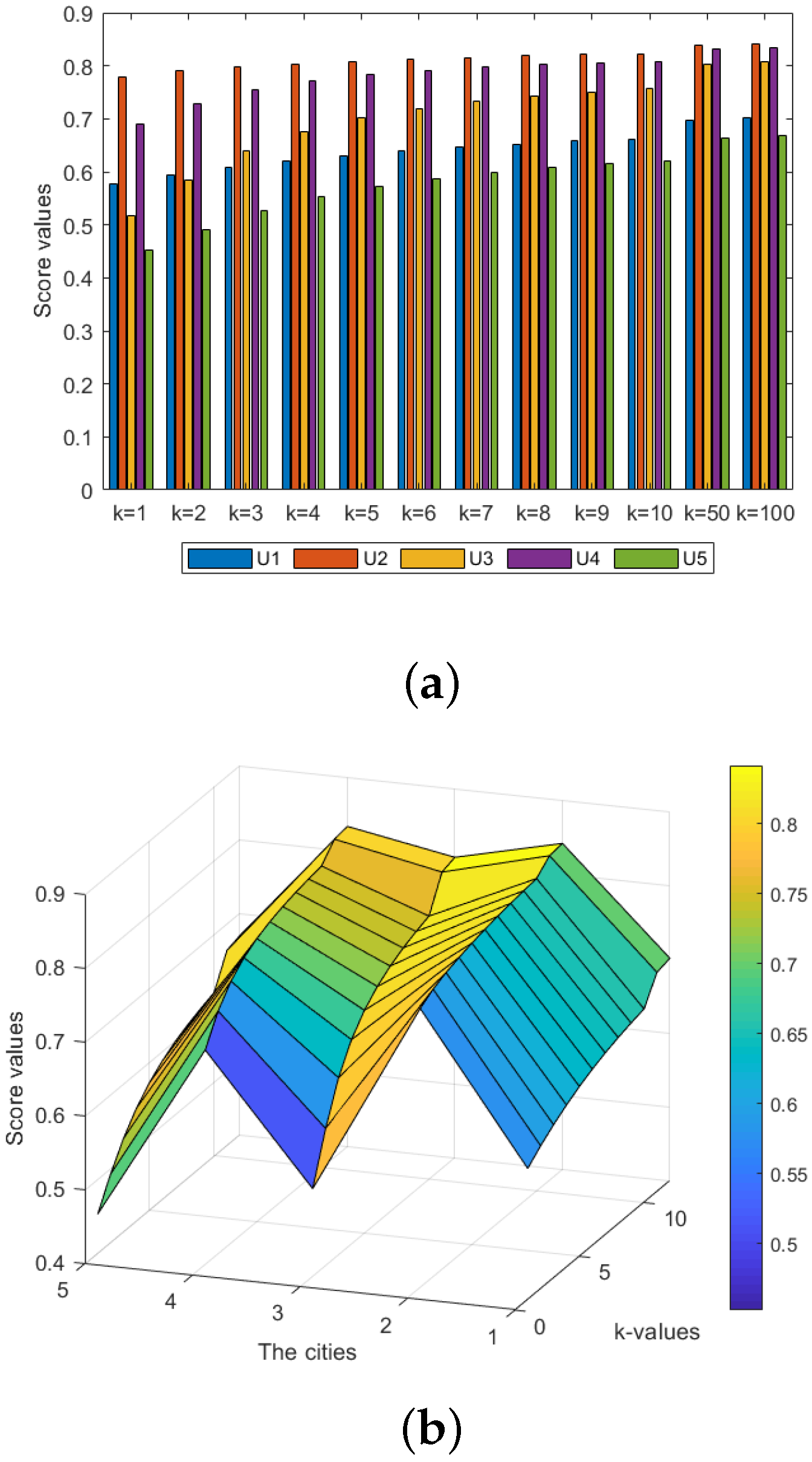
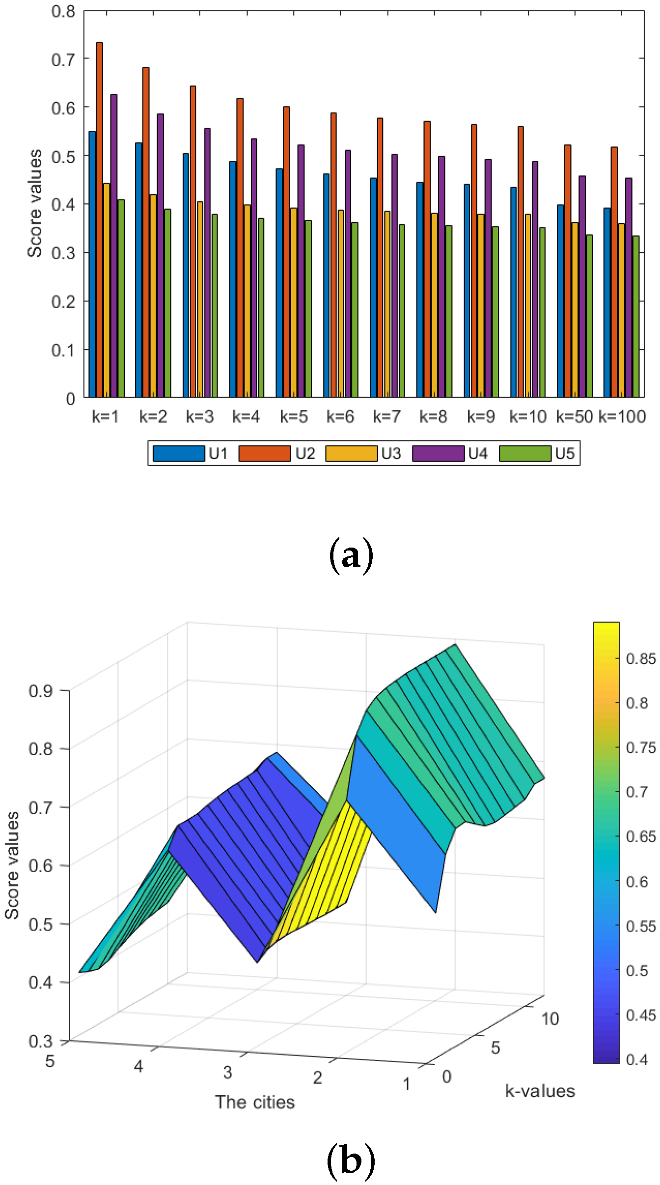
6.2.1. Effect of Parameter k

To capture the impact of the parameter k, we substitute different k-values into the HF Aczel–Alsina power model to obtain the ranking of cities affected by the storm. The results are presented in

Table 4. Scores and ranking results from HFAAPWA operations with different k-values.

$\Phi$	${\mathit{U}}_1$	${\mathit{U}}_2$	${\mathit{U}}_3$	${\mathit{U}}_4$	${\mathit{U}}_5$	Ranking Results
$k=1$	0.5772	0.7782	0.5184	0.6904	0.4525	$U_2\succ U_4\succ U_1\succ U_3\succ U_5$
$k=2$	0.5934	0.7899	0.5855	0.7287	0.4920	$U_2\succ U_4\succ U_1\succ U_3\succ U_5$
$k=3$	0.6074	0.7977	0.6395	0.7547	0.5259	$U_2\succ U_4\succ U_3\succ U_1\succ U_5$
$k=4$	0.6196	0.8037	0.6766	0.7717	0.5523	$U_2\succ U_4\succ U_3\succ U_1\succ U_5$
$k=5$	0.6301	0.8085	0.7018	0.7833	0.5722	$U_2\succ U_4\succ U_3\succ U_1\succ U_5$
$k=6$	0.6390	0.8126	0.7195	0.7915	0.5873	$U_2\succ U_4\succ U_3\succ U_1\succ U_5$
$k=7$	0.6465	0.8160	0.7326	0.7975	0.5988	$U_2\succ U_4\succ U_3\succ U_1\succ U_5$
$k=8$	0.6527	0.8188	0.7425	0.8021	0.6078	$U_2\succ U_4\succ U_3\succ U_1\succ U_5$
$k=9$	0.6579	0.8212	0.7503	0.8057	0.6150	$U_2\succ U_4\succ U_3\succ U_1\succ U_5$
$k=10$	0.6623	0.8232	0.7566	0.8086	0.6209	$U_2\succ U_4\succ U_3\succ U_1\succ U_5$
$k=50$	0.6974	0.8396	0.8017	0.8305	0.6641	$U_2\succ U_4\succ U_3\succ U_1\succ U_5$
$k=100$	0.7018	0.8417	0.8071	0.8332	0.6696	$U_2\succ U_4\succ U_3\succ U_1\succ U_5$

and

Table 5. Scores and ranking results from HFAAPWG operations with different k-values.

$\Psi$	${\mathit{U}}_1$	${\mathit{U}}_2$	${\mathit{U}}_3$	${\mathit{U}}_4$	${\mathit{U}}_5$	Ranking Results
$k=1$	0.5485	0.7322	0.4434	0.6267	0.4075	$U_2\succ U_4\succ U_1\succ U_3\succ U_5$
$k=2$	0.5257	0.6807	0.4185	0.5854	0.3893	$U_2\succ U_4\succ U_1\succ U_3\succ U_5$
$k=3$	0.5044	0.6425	0.4053	0.5555	0.3779	$U_2\succ U_4\succ U_1\succ U_3\succ U_5$
$k=4$	0.4866	0.6171	0.3971	0.5352	0.3704	$U_2\succ U_4\succ U_1\succ U_3\succ U_5$
$k=5$	0.4725	0.5996	0.3916	0.5212	0.3652	$U_2\succ U_4\succ U_1\succ U_3\succ U_5$
$k=6$	0.4614	0.5869	0.3875	0.5110	0.3613	$U_2\succ U_4\succ U_1\succ U_3\succ U_5$
$k=7$	0.4527	0.5774	0.3843	0.5032	0.3582	$U_2\succ U_4\succ U_1\succ U_3\succ U_5$
$k=8$	0.4456	0.5700	0.3817	0.4971	0.3558	$U_2\succ U_4\succ U_1\succ U_3\succ U_5$
$k=9$	0.4399	0.5641	0.3796	0.4921	0.3537	$U_2\succ U_4\succ U_1\succ U_3\succ U_5$
$k=10$	0.4351	0.5593	0.3777	0.4881	0.3520	$U_2\succ U_4\succ U_1\succ U_3\succ U_5$
$k=50$	0.3972	0.5221	0.3609	0.4567	0.3357	$U_2\succ U_4\succ U_1\succ U_3\succ U_5$
$k=100$	0.3924	0.5173	0.3586	0.4526	0.3335	$U_2\succ U_4\succ U_1\succ U_3\succ U_5$

as well as Figure 1 and Figure 2.

Table 4 demonstrates a consistent increase in the scores of each city obtained by the HFAAPWA operator as the k-value increases. When $k=1$ or 2, the ranking is $U_2\succ U_4\succ U_1\succ U_3\succ U_5$, and when k takes any other values the ranking is $U_2\succ U_4\succ U_3\succ U_1\succ U_5$. Similarly, Table 5 shows a steady decrease in scores obtained by the HFAAPWG operator as the k-value increases. The ranking of cities remains unchanged with varying k-values and is consistently $U_2\succ U_4\succ U_1\succ U_3\succ U_5$. The highest and lowest scores obtained by both operators are identical, providing valuable information for decision-makers.

Furthermore, based on Figure 1 and Figure 2, we can deduce that, when different k-values are substituted, the final sorting results remain unchanged. The consistency in the sorting results serves as evidence for the robustness of the proposed HFAAPWA and HFAAPWG operators.

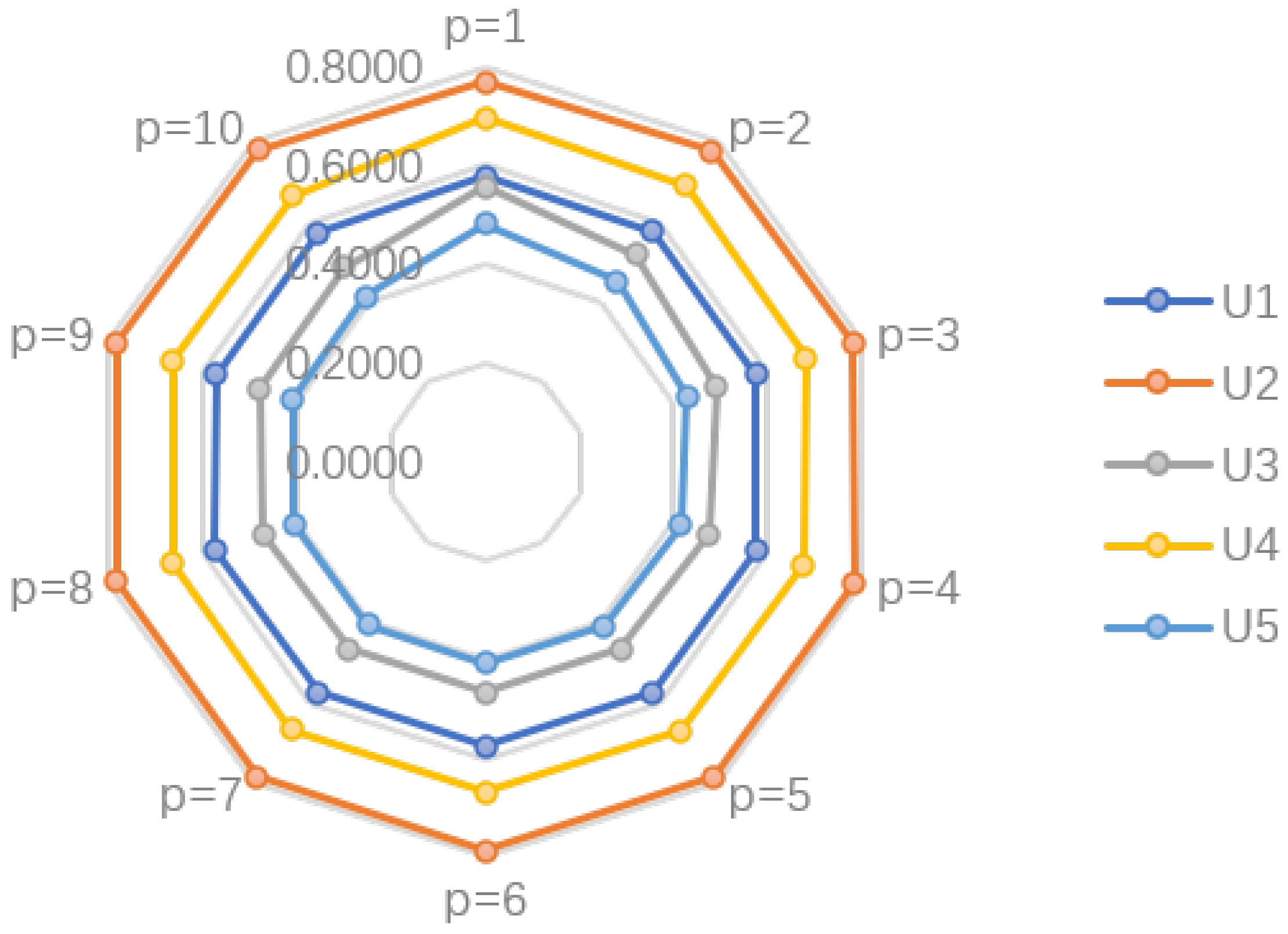
6.2.2. Effect of Parameter p

Similarly, substituting different p-values into the model, the scores and rankings of the two operations are summarized in

Table 6. Scores and ranking results from HFAAPWA operations with different p-values.

$\Phi$	${\mathit{U}}_1$	${\mathit{U}}_2$	${\mathit{U}}_3$	${\mathit{U}}_4$	${\mathit{U}}_5$	Ranking Results
$p=1$	0.5764	0.7690	0.5556	0.6971	0.4812	$U_2\succ U_4\succ U_1\succ U_3\succ U_5$
$p=2$	0.5772	0.7782	0.5184	0.6905	0.4525	$U_2\succ U_4\succ U_1\succ U_3\succ U_5$
$p=3$	0.5769	0.7836	0.4905	0.6821	0.4298	$U_2\succ U_4\succ U_1\succ U_3\succ U_5$
$p=4$	0.5763	0.7861	0.4742	0.6754	0.4158	$U_2\succ U_4\succ U_1\succ U_3\succ U_5$
$p=5$	0.5756	0.7869	0.4668	0.6711	0.4085	$U_2\succ U_4\succ U_1\succ U_3\succ U_5$
$p=6$	0.5751	0.7867	0.4653	0.6684	0.4057	$U_2\succ U_4\succ U_1\succ U_3\succ U_5$
$p=7$	0.5746	0.7859	0.4677	0.6669	0.4057	$U_2\succ U_4\succ U_1\succ U_3\succ U_5$
$p=8$	0.5741	0.7847	0.4727	0.6659	0.4074	$U_2\succ U_4\succ U_1\succ U_3\succ U_5$
$p=9$	0.5736	0.7831	0.4792	0.6654	0.4103	$U_2\succ U_4\succ U_1\succ U_3\succ U_5$
$p=10$	0.5732	0.7813	0.4868	0.6650	0.4140	$U_2\succ U_4\succ U_1\succ U_3\succ U_5$

and

Table 7. Scores and ranking results from HFAAPWG operations with different p-values.

$\Psi$	${\mathit{U}}_1$	${\mathit{U}}_2$	${\mathit{U}}_3$	${\mathit{U}}_4$	${\mathit{U}}_5$	Ranking Results
$p=1$	0.5416	0.7135	0.4681	0.6224	0.4290	$U_2\succ U_4\succ U_1\succ U_3\succ U_5$
$p=2$	0.5485	0.7322	0.4434	0.6267	0.4075	$U_2\succ U_4\succ U_1\succ U_3\succ U_5$
$p=3$	0.5544	0.7455	0.4267	0.6302	0.3925	$U_2\succ U_4\succ U_1\succ U_3\succ U_5$
$p=4$	0.5582	0.7527	0.4175	0.6325	0.3840	$U_2\succ U_4\succ U_1\succ U_3\succ U_5$
$p=5$	0.5604	0.7555	0.4133	0.6334	0.3782	$U_2\succ U_4\succ U_1\succ U_3\succ U_5$
$p=6$	0.5613	0.7555	0.4122	0.6334	0.3782	$U_2\succ U_4\succ U_1\succ U_3\succ U_5$
$p=7$	0.5616	0.7535	0.4130	0.6328	0.3782	$U_2\succ U_4\succ U_1\succ U_3\succ U_5$
$p=8$	0.5614	0.7504	0.4151	0.6317	0.3793	$U_2\succ U_4\succ U_1\succ U_3\succ U_5$
$p=9$	0.5610	0.7464	0.4180	0.6303	0.3810	$U_2\succ U_4\succ U_1\succ U_3\succ U_5$
$p=10$	0.5603	0.7419	0.4215	0.6288	0.3831	$U_2\succ U_4\succ U_1\succ U_3\succ U_5$

as well as Figure 3 and Figure 4.

Combining Table 6 and Table 7 as well as Figure 3 and Figure 4, the ranking results of both operators are $U_2\succ U_4\succ U_1\succ U_3\succ U_5$ for different p-values. Obviously, the scoring values of the five cities change only slightly with the change in p-values, while the ranking results are consistent. This reflects that the results are stable, which in turn indicates the robustness of the model.

Upon review of the preceding discourse, it becomes evident that the primary outcomes derived from varying parameter values exhibit a high degree of concordance. This observation underscores the robustness of the operations proposed and attests to the stability inherent within the model.

6.3. Comparative Analysis

To demonstrate the validity and advantages of the model, the presented model is compared with several extant models, including the HFWA operator and HAWG operator [14], the HFEWA operator and HFEWG operator [17], the HFDWA operator and HFDWG operator [18], the HFAAWA operator and HFAAWG operator, and the HFAAWBM operator [20]. The comparison results are shown in

Table 8. Comparison result.

Techniques	t-Norm Used	Parameter	Weight	Preference Order
HFWA [14]	No	No	Assumed	$U_2\succ U_4\succ U_3\succ U_1\succ U_5$
HFWG [14]	No	No	Assumed	$U_2\succ U_4\succ U_1\succ U_3\succ U_5$
HFEWA [17]	Einstein	No	Assumed	$U_2\succ U_4\succ U_3\succ U_1\succ U_5$
HFEWG [17]	Einstein	No	Assumed	$U_2\succ U_4\succ U_1\succ U_3\succ U_5$
HFDWA [18]	Dombi	1	Assumed	$U_2\succ U_4\succ U_3\succ U_1\succ U_5$
HFDWG [18]	Dombi	1	Assumed	$U_2\succ U_4\succ U_1\succ U_3\succ U_5$
HFAAWA [20]	Aczel–Alsina	1	Assumed	$U_2\succ U_4\succ U_3\succ U_1\succ U_5$
HFAAWG [20]	Aczel–Alsina	1	Assumed	$U_2\succ U_4\succ U_1\succ U_3\succ U_5$
HFAAWBM [20]	Aczel–Alsina	3	Assumed	$U_2\succ U_4\succ U_1\succ U_3\succ U_5$
Proposed method	Aczel–Alsina	2	Entropy weights	$U_2\succ U_4\succ U_1\succ U_3\succ U_5$
(HFAAPWA)			and power operator
Proposed method	Aczel–Alsina	2	Entropy weights	$U_2\succ U_4\succ U_1\succ U_3\succ U_5$
(HFAAPWG)			and power operator

. Invariably, different methods yield the same first and last rankings, which shows that the proposed method is effective. Based on the comparison, here are some advantages of the proposed model:

(1) In our model, the Chi-square distance measure with a strong statistical background is utilized to portray the correlation and dissimilarity between data. In addition, in contrast to the mentioned models, the weights of the present model are not given directly by the decision-maker, but the objective weights are calculated using the Shannon entropy weighted method and optimally adjusted by the power operator.

(2) Compared with the models proposed by Xia and Xu [14], Yu [17], He [18] based on weighted operations, Einstein operations, and Dombi operations, the alternatives ranking obtained by the HF power Aczel–Alsina model proposed in this paper based on Aczel–Alsina operations is more reasonable.

(3) In contrast to the models proposed by Xia and Xu [14], and Yu [17], our model due to the introduction of the parameters p and k, which can be changed according to the real demand, add flexibility and generality to the model.

7. Conclusions

In this paper, a novel HF aggregation operation model is proposed and used in a multi-attribute decision-making problem. This approach extends the utilization of the Chi-squared distance and concurrently refreshes a method for optimizing weights in hesitant fuzzy sets, integrating the merits of the Aczel–Alsina operators into HFSs, thereby providing novel insights for existing research. Consequently, the effectiveness, flexibility, and justification of the method is verified by case illustration and experimental analysis. The main contributions of this paper are distilled below:

(1) This paper extends the Chi-square distance to HFSs and proposes the HF generalized Chi-square distance and corresponding similarity measures. Moreover, it is applied in the entropy weight method to obtain the weights, which assists in improving the accuracy of the weights.

(2) This study examines the interplay of data support through power operations to optimize attribute weights. By integrating these weights with the highly flexible Aczel–Alsina operators, we introduce the HF Aczel–Alsina power model. This model provides a novel and robust approach to the field of multi-attribute decision-making.

Notably, the model is applicable not only to the problem of ranking the impact of storms on cities, but also to more MADM problems. In addition, the model has some drawbacks. In general, there are three approaches to standardize the length of HFEs, which are positive attitude (risk-seeking), negative attitude (risk-averse), and compromise treatment (risk-neutral) complement. This paper only chooses the positive attitude complementation method, i.e., repeating the maximum value of the HFE, which may lead to duplicate values in the aggregated HFE. Subsequent research can make improvements based on this shortcoming. Moving forward in further research, given the extensive and robust applications of machine learning across various domains, it is pertinent to explore the potential of harnessing machine learning techniques to simplify and enhance the model. This helps to solve practical problems more effectively and improve decision-making efficiency, such as applying aggregation algorithms in large-scale group decision-making problems. Moreover, this paper does not delve into the psychological and behavioral tendencies of decision-makers, nor the impact of these factors on the decision-making process. Future work will concentrate on regret theory, prospect theory, and other methodologies that more accurately capture the psychological aspects of decision-makers. By addressing these two dimensions, future studies can investigate how to integrate machine learning and psychological factors to bolster the effectiveness and applicability of decision-making.

References

1. Zadeh, L. Fuzzy sets. Inf. Control. 1965, 8, 338–353. [Google Scholar] [CrossRef]
2. Dalman, H.; Güzel, N.; Sivri, M. A fuzzy set-based approach to multi-objective multi-item solid transportation problem under uncertainty. Int. J. Fuzzy Syst. 2016, 18, 716–729. [Google Scholar] [CrossRef]
3. Dubois, D.; Prade, H.; Esteva, F. Fuzzy set modelling in case-based reasoning. Int. J. Intell. Syst. 1998, 13, 345–373. [Google Scholar] [CrossRef]
4. Atanassov, K.; Stoeva, S. Intuitionistic fuzzy sets. Fuzzy Sets Syst. 1986, 20, 87–96. [Google Scholar] [CrossRef]
5. Yager, R.; Abbasov, A. Pythagorean membership grades, complex numbers, and decision making. Int. J. Intell. Syst. 2013, 28, 436–452. [Google Scholar] [CrossRef]
6. Torra, V. Hesitant fuzzy sets. Int. J. Intell. Syst. 2010, 25, 529–539. [Google Scholar] [CrossRef]
7. Al-shami, T. (2,1)-Fuzzy sets: Properties, weighted aggregated operators and their applications to multi-criteria decision-making methods. Complex Intell. Syst. 2023, 9, 1687–1705. [Google Scholar] [CrossRef]
8. Al-Shami, T.; Mhemdi, A. Generalized Frame for Orthopair Fuzzy Sets: (m,n)-Fuzzy Sets and Their Applications to Multi-Criteria Decision-Making Methods. Information 2023, 14, 56. [Google Scholar] [CrossRef]
9. Luo, M.; Zhao, R. A distance measure between intuitionistic fuzzy sets and its application in medical diagnosis. Artif. Intell. Med. 2018, 89, 34–39. [Google Scholar] [CrossRef]
10. Xu, Z.; Zhang, X. Hesitant fuzzy multi-attribute decision making based on TOPSIS with incomplete weight information. Knowl.-Based Syst. 2013, 52, 53–64. [Google Scholar] [CrossRef]
11. Zhang, N.; Wei, G. Extension of VIKOR method for decision making problem based on hesitant fuzzy set. Appl. Math. Model. 2013, 37, 4938–4947. [Google Scholar] [CrossRef]
12. Chen, N.; Xu, Z. Hesitant fuzzy ELECTRE II approach: A new way to handle multi-criteria decision making problems. Inf. Sci. 2015, 292, 175–197. [Google Scholar] [CrossRef]
13. Menger, K. Statistical metrics. Sel. Math. 2003, 2, 433–435. [Google Scholar]
14. Xia, M.; Xu, Z. Hesitant fuzzy information aggregation in decision making. Int. J. Approx. Reason. 2011, 52, 395–407. [Google Scholar] [CrossRef]
15. Yager, R. The power average operator. IEEE Trans. Syst. Man Cybern. Part Syst. Humans 2001, 31, 724–731. [Google Scholar] [CrossRef]
16. Xu, Z.; Yager, R. Power-geometric operators and their use in group decision making. IEEE Trans. Fuzzy Syst. 2009, 18, 94–105. [Google Scholar] [CrossRef]
17. Yu, D. Some hesitant fuzzy information aggregation operators based on Einstein operational laws. Int. J. Intell. Syst. 2014, 29, 320–340. [Google Scholar] [CrossRef]
18. He, X. Typhoon disaster assessment based on Dombi hesitant fuzzy information aggregation operators. Nat. Hazards 2018, 90, 1153–1175. [Google Scholar] [CrossRef]
19. Aczél, J.; Alsina, C. Characterizations of some classes of quasilinear functions with applications to triangular norms and to synthesizing judgements. Aequationes Math. 1982, 25, 313–315. [Google Scholar] [CrossRef]
20. Senapati, T.; Chen, G.; Mesiar, R. Novel Aczel—Alsina operations-based hesitant fuzzy aggregation operators and their applications in cyclone disaster assessment. Int. J. Gen. Syst. 2022, 51, 511–546. [Google Scholar] [CrossRef]
21. Senapati, T.; Chen, G.; Yager, R.R. Aczel—Alsina aggregation operators and their application to intuitionistic fuzzy multiple attribute decision making. Int. J. Intell. Syst. 2022, 37, 1529–1551. [Google Scholar] [CrossRef]
22. Senapati, T.; Mesiar, R.; Simic, V. Analysis of interval-valued intuitionistic fuzzy Aczel—Alsina geometric aggregation operators and their application to multiple attribute decision-making. Axioms 2022, 11, 258. [Google Scholar] [CrossRef]
23. Senapati, T. Approaches to multi-attribute decision making based on picture fuzzy Aczel-Alsina average aggregation operators. Comput. Appl. Math. 2022, 41, 1–28. [Google Scholar] [CrossRef]
24. Szmidt, E.; Kacprzyk, J. Distances between intuitionistic fuzzy sets. Fuzzy Sets Syst. 2000, 114, 505–518. [Google Scholar] [CrossRef]
25. Grzegorzewski, P. Distances between intuitionistic fuzzy sets and/or interval-valued fuzzy sets based on the Hausdorff metric. Fuzzy Sets Syst. 2004, 148, 319–328. [Google Scholar] [CrossRef]
26. Xu, Z.; Xia, M. Distance and similarity measures for hesitant fuzzy sets. Inf. Sci. 2011, 181, 2128–2138. [Google Scholar] [CrossRef]
27. Perlibakas, V. Distance measures for PCA-based face recognition. Pattern Recognit. Lett. 2004, 25, 711–724. [Google Scholar] [CrossRef]
28. Ren, H.; Xiao, S.; Zhou, H. A Chi-Square Distance-Based Similarity Measure of Single-Valued Neutrosophic Set and Applications; Infinite Study: Ghaziabad, India, 2019. [Google Scholar] [CrossRef]
29. Klement, E.; Mesiar, R.; Pap, E. Triangular Norms; Springer Science & Business Media: Berlin/Heidelberg, Germany, 2013. [Google Scholar] [CrossRef]
30. Senapati, T.; Simic, V.; Saha, A. Intuitionistic fuzzy power Aczel-Alsina model for prioritization of sustainable transportation sharing practices. Eng. Appl. Artif. Intell. 2023, 119, 105716. [Google Scholar] [CrossRef]
31. Alsina, C.; Schweizer, B.; Frank, M. Associative Functions: Triangular Norms and Copulas; World Scientific: Singapore, 2006. [Google Scholar] [CrossRef]
32. Torra, V.; Narukawa, Y. On hesitant fuzzy sets and decision. In Proceedings of the 2009 IEEE International Conference on Fuzzy Systems, Jeju Island, South Korea, 20–24 August 2009; IEEE: Piscataway, NJ, USA, 2009; pp. 1378–1382. [Google Scholar] [CrossRef]
33. Xia, M.; Xu, Z. Studies on the aggregation of intuitionistic fuzzy and hesitant fuzzy information. Int. J. Intell. Syst. 2011, 26, 26. [Google Scholar]
34. Yager, R. Generalized OWA aggregation operators. Fuzzy Optim. Decis. Mak. 2004, 3, 93–107. [Google Scholar] [CrossRef]
35. Farhadinia, B. Information measures for hesitant fuzzy sets and interval-valued hesitant fuzzy sets. Inf. Sci. 2013, 240, 129–144. [Google Scholar] [CrossRef]
36. Shannon, C. A mathematical theory of communication. Bell Syst. Tech. J. 1948, 27, 379–423. [Google Scholar] [CrossRef]
37. Xu, Z. Uncertain Multi-Attribute Decision Making: Methods and Applications; Springer: Berlin/Heidelberg, Germany, 2015. [Google Scholar] [CrossRef]
38. Stewart, C. An approach to measure distance between compositional diet estimates containing essential zeros. J. Appl. Stat. 2017, 44, 1137–1152. [Google Scholar] [CrossRef]
39. Zhou, H.; Ren, H. A study of intuitionistic fuzzy similarity clustering algorithm based on Chi-Square distance. J. Chongqing Univ. Technol. (Nat. Sci.) 2020, 34, 238–246. [Google Scholar]
Figure 1. Scores Φ ϕ for five cities at different k-values taken by the HFAAPWA operation when p = 2 . Changes are shown in bar chart (a) and three-dimensional graph (b).
Symmetry 16 01702 g001
Figure 2. Scores Ψ ϕ for five cities at different k-values taken by the HFAAPWG operation when p = 2 . Changes are shown in bar chart (a) and three-dimensional graph (b).
Symmetry 16 01702 g002
Figure 3. Scores Φ ϕ for five cities at different p-values taken by the HFAAPWA operation when k = 1 .
Symmetry 16 01702 g003
Figure 4. Scores Ψ ϕ for five cities at different p-values taken by the HFAAPWA operation when k = 1 .
Symmetry 16 01702 g004