Abstract
This paper addresses the robust stabilization problem of a cart–pole system. The controlled dynamics of this interconnected system are deduced by following the analytic framework of Lagrangian mechanics, and the residual terms are formulated as a bias depending on the angle and angular velocity. A geometric definition of Proportional–Integral–Derivative (PID) control algorithm is proposed, and a Lyapunov function is explicitly constructed through two stages of variable change. Local exponential stability of the stable equilibrium is proved, and a criterion for parameter tuning is provided by ensuring an exponential decrease in the Lyapunov function. Enlarging the control parameters to infinity allows for the extension of attraction region almost to the half circle. The effectiveness of geometric PID controller and the local exponential stability of the resulting close system are verified by simulating a numerical example.
1. Introduction
Stabilization of a cart–pendulum (cart–pole) system is of significant interest for both practical applications in control engineering and scientific research of control theory [1,2]. Attitude control of a spacecraft booster is precisely a stabilization problem of the cart–pendulum. Balancing of a two-wheeled cart in robotic engineering also involves stabilizing an inverted pendulum on a cart. Due to the nonlinear nature of the cart–pendulum system, it has been a popular benchmark for the invention, validation and verification of many advanced nonlinear control techniques, especially for the energy-based control [3,4,5,6,7]. As an under-actuated system, the cart–pole system has two dimensions of freedom for motion, i.e., the pendulum angle and cart position, but is actuated, in only one dimension, by forces applied to the cart. This property has inspired the researchers to study the cart–pole system as an interconnected or cascade system and use the energy-based method of Interconnection and Damping Assignment Passivity-Based Control (IDA-PBC) to get the pending position stabilized [4,5]. Another point of view for understanding the dynamics of a cart–pole system is by following the framework of the Lagrangian mechanics. In this line, the energybased method of controlled Lagrangian is introduced to stabilize an inverted pendulum by shaping the kinetic or potential energy such that some geometric structures of Lagrangian system are matched [6,7]. In the present paper, we establish the controlled dynamics of a cart–pendulum system in the analytic framework of Lagrangian mechanics, which allows us to investigate the interactions between the pending pole and the tracking cart.
Among the various control techniques developed for a cart–pole system, more advanced approaches, such as energy-based control [3,4,5,6,7] or model predictive control [8], are based on system model and are advantageous in providing more accurate control, as simulation and computation of physical models are possible. More recent results are established on the data-driven technique of learning-based control. The algorithm of Deep Reinforcement Learning (DRL) allows for online extraction of the system model [9,10] or real-time identification of the optimal parameters [11,12] from the collected data. Therefore, the DRL method has significant advantages in providing an adaptive controller by which seeking optimal solutions and improving the robustness to time-varying disturbances are possible. Although the learning-based control has relaxed, more or less, the requirement of exact model knowledge, its training process relies heavily on a large amount of data. As another model-free method, however, PID control has its strength in simplifying the structure of the controller and reducing the requirement for information about the system model. In the algorithm of PID control, the input commands are formed by combining a proportion, a time derivative and a time integral of errors. Computing those actions is straightforward in vector spaces. For a system defined in a non-Euclidean space, however, the classical definition of PID control makes no mathematical sense and providing a rigorous and consistent extension of the conventional one to more general settings requires further studies. The work in [13] provided a geometric PD controller for simple mechanical systems evolving on Riemannian manifolds by using a negative proportion of the gradient of an error function as the proportional action. In this line, a left-invariant definition of PID controller was proposed for fully actuated systems evolving on Lie groups by identifying the integral action in Lie algebra as an integration of PD commands along time [14,15]. A parallel work in [16] focused on the extension of PID to more geometric settings, in which an intrinsic PID controller is defined with all the input commands justified using the notation of covariant derivative. We also attempted to generalize the capability of geometric PID control to stabilize under-actuated systems like steering-controlled vehicles. This extension, however, requires modification on the definition of integral action [17]. To our knowledge, this is the first time confirming the effectiveness of geometric PID control law in robust stabilization of under-actuated systems, i.e., stabilizing the variables in the under-actuated dimension of an interconnected system, like a cart–pole system, despite the influence of residual terms that come from the interactions between actuated and under-actuated dimensions.
Although the design of the geometric PID control has been studied for a decade, the convergence analysis for geometric PID-controlled systems needs further studies. Two aspects are worthy of deeper investigation. First, most results were developed by associating a feed-forward control with the geometric PID control [16,18]. The feed-forward action still needs the exact information of system model. The work in [14] suggests the simplest design only with PID inputs, while the feed-forward compensation is not necessary. In this line, we are inspired to propose a modeling of a cart–pole system in which the residual term is viewed as a bias to be countered by integral action rather than a term to be compensated by feed-forward control. The convergence analysis for this geometric PID-controlled system is not straightforward. The integral control must be ensured with the ability to deal with both state-dependent and velocity-dependent biases. To our knowledge, using integral action to compensate for the time-varying effects caused by residual terms in a cart–pendulum system has not been studied in the existing literature. Second, regarding the convergence, only Asymptotic Stability (AS) was established in previous works [14,15,16,18], and the proof must be resolved in association with LaSalle’s invariance principle. We want to establish a stronger result of Exponential Stability (ES) for a geometric PID-controlled cart–pole system. Our goal is to provide an analytical framework in which integral action is confirmed to be able to completely attenuate the effects of both state-dependent and velocity-dependent biases.
The contributions of this paper are in following aspects:
- The controlled dynamics of a cart–pole system is presented in a form of Euler–Lagrangian equations and the residual terms are viewed as state-dependent and velocity-dependent biases whose effects are not necessarily required to be compensated by feed-forward control.
- The process of controller design is simplified as defining a geometric PID control algorithm for an inverted pendulum. The proposed control law allows for robust stabilization of angles to an arbitrary value, as integral action is incorporated to suppress the effects caused by residual terms. The advantage of derivative control in accelerating convergence speed and the strength of integral action in compensating unknown biases are confirmed.
- A Lyapunov function is deduced by applying two stages of coordinate change. Conditions for the tuning of controller parameters are justified by guaranteeing exponential decrease in the established Lyapunov function. The attraction region is enlarged almost to a half circle.
The remaining contents of this paper are outlined as follows: In Section 2, the mathematical model of a cart–pole system is established and its governing equations of controlled dynamics are derived. In Section 3, a geometric PID controller is proposed. The main attention of the present paper is focused on providing a rigorous convergence analysis; see Section 4 for detailed proof. Results of numerical simulation are reported and the limitations are discussed in Section 5, followed by the conclusion in Section 6.
2. System Modeling
As shown in Figure 1, a cart–pole is an interconnected system with physical interaction between a cart and a pole. One end of the rob is pivoted on the base of the cart, and the other end is associated with a ball. The cart and ball are of mass M and m, respectively, while the rob is assumed to be massless. We denote by the angle between the rob and the vertical line, which needs to be stabilized. The cart is controlled by an external force . Because of the action by the gravity of the earth, it is difficult to keep the rob staying in an upright direction, as is an unstable equilibrium point for a cart–pole system of no control, and arbitrarily small deviation from this point will let the ball fall down. Applying control in the horizontal direction to the cart, however, allows us to have the angle stabilized to a desired equilibrium. In this section, an explicit expression for the governing equation is deduced by following the analytical framework of Lagrangian mechanics [6].
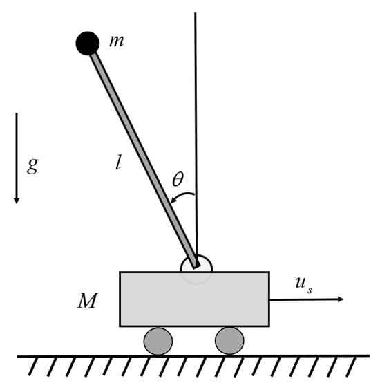
Figure 1.
Model of a cart–pole system.
Summing up the kinetic energy of ball and cart gives the total value of kinetic energy
The potential energy only appears in the component of the ball
Accordingly, the Lagrangian for a cart–pole system is obtained
The resulting Euler–Lagrangian equations follow
Replacing the partial derivatives with explicit computations gives a more detailed representation of Euler–Lagrangian equations
whose solutions are
By defining a new variable
a more compact form for the dynamics of variable turns out to be
where the residual term comes from the action by gravity of the earth, and the interactions between the cart and the pole
Instead of compensating the influence of this residual term through feed-forward control, we let it appear as a state-dependent and velocity-dependent bias in the system model and attempt to obtain its effects attenuated by incorporating integral action in the process of controller design.
3. Design of Geometric PID Controller
As shown in Figure 2, the system is actuated on the cart, and the feedback is based on the measurements of angle and angular velocity on the pending pole. The geometric design of PID control law is different from the conventional design in Euclidean spaces. First, the measurements must be transformed, through some geometric computations, into a geometric object of the gradient vector. Second, the proportional, integral, and derivative inputs must be defined in vector form. Thus, the geometric PID controller is defined as
where represents angular velocity, the proportional command is proportional to the gradient of error function , and is a time integral of and derivative commands . Submitting the control inputs into Equation (2) results into a closed system

Figure 2.
Diagram of a geometric PID-controlled cart–pole system.
The goal for controller design is settled as to stabilize the pair of states to a desired equilibrium of . Without loss of generality, we take in the following analysis, as the problem of stabilizing towards an arbitrary target point of is equivalent to that of driving to . We do not include the requirements for the specification of states in our controller design. It is clear that, when , there exist a term in , which only vanishes when . This implies that, when the target point , the cart will keep constantly accelerating such that the pole remains at the equilibrium point.
4. Convergence Analysis
In order to achieve the proof of exponential stability, the resulting close system needs a representation in some renewed coordinate systems. Fortunately, it is possible to construct the proper coordinates by justifying two stages of reasonable variable change. In the first step, it is shown that there exists a negative proportion of in the time derivative of , which implies the gradient-descent decline of an error function. The second-stage variable change further ensures that the derivative input and the integral action exponentially approach the proportional one and the bias , respectively. Provided the results of two-stage coordinate change, it is straightforward to come up with a Lyapunov candidate whose decrease proves the exponential stability.
4.1. First-Stage Variable Change
It is difficult to judge the stability of the resulting system in the original coordinate . By choosing the new variables , we update the coordinate system as
Computing its inverse allows us to represent , , and in terms of x and y:
with , . With the help of this variable change, the original system is turned into that described in the new coordinates:
By defining vectors , we obtain a system in linear form:
where the matrix and the vectors , are
After performing the first step of variable change, the resulting representation in the renewed coordinate system is obtained in the next proposition.
Proposition 1.
Suppose that and . Then, the geometric PID-controlled system (4)–(6) has a representation of the form (9) and (10) under the coordinate change (7) and (8). The norm of vectors and is upper bounded by the values of and
with
and
Proof of Proposition 1.
The above computations have established the updated representation of the geometric PID-controlled system in the renewed coordinates. We need to further identify the upper bound for the norm of vectors and . From their expressions in (12), we have with ; and we also know that
The remaining task then turns out to be estimating the upper bounds of and . Computing the derivative of gives
In order to obtain the estimate of , we need to know the upper bounds of , , . With the expression of in (1), we have
Further, with the expression of in (3), we obtain
where we have used the facts in (17) and (18) and the assumption on . Now, we are ready to obtain the upper bound for
Submitting the results from (16) and (19) into Equation (15) yields
where
and the values of are justified accordingly. □
The results in the first step of coordinate change have shown the fact that there exists a term in the time derivative of error function , which ensures a gradient-descent decline of . However, the term is not guaranteed to hold a negative value for arbitrary non-zero vectors. Thus, a second-stage variable change must be performed to obtain a reasonable coordinate system through a similar transformation. i.e., and , such that the term is ensured being definitely negative for all the vectors .
4.2. Second-Stage Variable Change
The second-stage process of variable change is to perform a similar transformation of the matrix . We let and turn the matrix in (11) into
This matrix has two eigenvalues
with having explicit expressions
which, indeed, are two solutions of the following equation:
The second-stage process of variable change is then defined as
or, in matrix form, as for . The matrix P then follows
We further obtain a transformation of the system (9) and (10) into that, described in terms of , and
where the matrix and vectors , are
By performing the second step of variable change, the form of resulting system is reported in the next proposition.
Proposition 2.
Suppose that Proposition 1 holds and γ is settled such that . Then, there exists a variable change (22) and (23), such that the system (9) and (10) has a representation of the form (24) and (25). The terms , and are bounded as follows:
with
Proof of Proposition 2.
By following the above computations, it is not difficult to obtain the renewed representation of the geometric PID-controlled system after two stages of variable change. The remaining task is to provide the estimate of upper bounds for , and . By Equations (20) and (21), we know that
Following Equation (26), we further obtain the result
by which in (28) is justified accordingly. By investigating the explicit solutions for in (21), we know the facts
By following Gershgorin circle theorem, we are allowed to come up with the estimate of upper bounds for , and ,
From (13) and (27), we know that
The vector can be viewed as a combination of two terms and . With the result of (14) in Proposition 1, we have
With the above results at hand, we can make a progress to reach (29) and (30) for the upper bounds of and with the values of and justified accordingly. □
4.3. Local Exponential Stability
With the above results obtained through two stages of coordinate change, it is sufficient to present the main results of this paper in the next theorem.
Theorem 1.
Suppose that the control parameters are settled as identifying and taking sufficiently large , with satisfying , then the desired stable equilibrium point of the system (4)–(6) is locally exponentially stable. Starting from an arbitrarily specified initial point in the attraction region with , and by declining the Lyapunov function,
the system’s states are stabilized to the stable equilibrium point, while the bias is countered by the integral action . Sufficiently large control parameters and allow us to extend the attraction region almost to the set of .
Proof of Theorem 1.
Computing the time derivative of (31) and replacing the terms and with (24) and (25) leads to
The results of (28)–(30) established in Proposition 2 allow us to obtain
By defining , we further have
with the matrix
By Gershgorin circle theorem, requires
By replacing with explicit expressions, we rewrite the conditions as
with . The above requirements are possible to be reached by taking appropriate control parameters and setting a proper value for the weight . Firstly, we set the proportional action with a of large value such that . Once is specified, enlarging the value of allows us to satisfy the condition (33). Next, given the fixed value of and , we are allowed to let the condition (34) be satisfied by choosing a sufficiently large value for .
Before proving the exponential stability, we first need to make sure that there exist two positive matrices and such that
Now, we want to prove that is lower bounded by . Actually, from the fact that at , we can view the values of and for arbitrary as path integrals along a curve parameterized by , with starting point at initial time and ending point at last time . As the path integrals are independent of the specific curves, we take the special one whose velocity equals the gradient of error function as the candidate path.
As , we further obtain
We can take a sufficiently small such that
As we know that , we can make sufficiently close to 1, and take such that
is satisfied for any in an arbitrarily given attraction region. The matrices in (35) are settled as and . The conditions (32) and (35) allow us to conclude that the desired equilibrium point is exponentially stable [19].
Next, we prove the extension of the attraction region. We need to ensure that does not reach a and does not exceed the value of H, i.e., and are always satisfied for all t. Let and , then we need to prove that and implies . As for all and ; we thus obtain the estimate of upper bound for
with
We further obtain the value of H justified as follows
The nominal part actually represents a physical model of damped oscillator. Enlarging the parameter to infinity will increase the frequency of the oscillator to infinity, and therefore allows us to reduce the period T to zero. Thus, it is possible to make the value of over a period stay sufficiently close to that of , i.e.,
Given an arbitrarily specified value of (sufficiently close to 1), by making sufficiently large, a real value of a satisfying can be justified such that indicates for all . Through a period, the accumulated effects by the term in is averaged out, while the total effects by the action of decreases the value of error function , i.e., . Therefore, the condition also remains valid for all , and the angles are ensured to be not exceeding the value of , which further determines the value of .
Now, it is sufficient to draw a conclusion on the extension of attraction region, i.e., enlarging the value of control parameters to infinity allows for an extension of attraction region almost to the set of . □
5. Results and Discussion
In this section, the numerical results of a simulating example are reported, and the limitations of the proposed design are discussed.
5.1. Results of Simulation
We verify the effectiveness of the proposed geometric PID control algorithm in robustly and exponentially stabilizing an inverted pendulum by providing a numerical simulation of a cart–pole system. The setting for the system model, control parameters, and coefficient of the Lyapunov function are presented in Table 1. The system is assumed to start from an initial point of with zero velocity and without integral action, i.e., .

Table 1.
Parameter setting of simulated cart–pole system.
Figure 3 shows the evolution of angle, angular velocity, and . As time evolves, the pair is stabilized to a specified value of targeted equilibrium point, i.e., in this case. Note that the cart is accelerating at this equilibrium, as . As the angle evolves, the -dependent variable varies, but with all its values being ensured to stay in a positive interval.

Figure 3.
Evolution the angle , the angular velocity , and the variable over time.
Figure 4 shows the evolution of control commands and bias. After a very short time of initial transient, the derivative input tends to the negative of proportional input , implying that is forced to hold the value of rapidly. This behavior confirms the fact that the derivative control is able to track the gradient of an error function. The benefit of using PD control is then obviously straightforward: forcing the system to satisfy the constraint leads into a gradient-descent decline of the error function, i.e., . Similarly, the integral part of actions rapidly approaches the opposite of the biased term after a short time of initial transient. This result indicates the advantages of integral control in dynamically rejecting the residual terms, rather than only compensating for the effect caused by steady-state errors.

Figure 4.
Evolution of the control inputs and the bias over time.
Figure 5 provides the evolution of Lyapunov function along time. As its value decreases to zero, the values of error function and (or equivalently ) approach zero. In other words, the states of system are driven to the stable equilibrium point , while the effects of biases are exactly attenuated by the integral action . The simulation results have verified the effectiveness of the proposed geometric design of PID control algorithm, i.e., achieving (at least locally) robust and exponential stabilization of an inverted pendulum system. The requirement of feed-forward control is relaxed, as an integral term is incorporated to deal with the influence of residual terms.
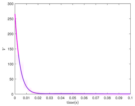
Figure 5.
Evolution of the Lyapunov function V over time.
5.2. Discussion of Limitations
There are two significant limitations to the analytical and simulating results in the present paper. First, although the exponential stability was proved in convergence analysis and was verified in simulations, its convergent speed is limited by , which is reduced to an infinitely small value when is enlarged sufficiently. Overcoming this limitation requires a new framework of analysis, which might suggest a completely different set of control parameters. Second, the cart–pole system consists of two one-dimensional sub-systems of cart and pole. Restricting our attention to this single-dimensional case simplifies both the convergence analysis and simulation experiment. It is worth future interest to extend this result to more general settings for interconnected systems evolving on nonlinear spaces of multiple dimensions, e.g., for an inverted spherical pendulum whose configuration space involves a two-dimensional manifold [20] and for pendubots with multiple linkages on the pendulum [21,22].
6. Conclusions
This paper proposes a geometric PID controller for robust and exponential stabilization of a cart–pole system. The controlled dynamics are deduced by following an analytic framework of Lagrangian mechanics, in which the interconnections are clearly presented. Next, we formulate the residual term as a biased term depending on both angle and angular velocity. A geometric PID control strategy is provided to stabilize the system’s state to a desired equilibrium point despite the influence of biases. In the proposed controller algorithm, the proportional part of actions is defined as a negative proportion of the gradient of an error function, while the integral part is justified as an integration of proportional-derivative commands along time. A Lyapunov metric is constructively established by performing two stages of coordinate change, and local exponential stability is proved for the closed system. Conditions for parameter tuning are obtained by ensuring the exponential decline of the suggested Lyapunov candidate. Our next interest in future research is to accelerate the convergence speed and to consider more complicated cases of multiple dimensions.
Author Contributions
Conceptualization, Z.Z., M.F. (Miaoxu Fang) and M.F. (Minrui Fei); methodology, Z.Z. and J.L.; formal analysis, Z.Z. and M.F. (Miaoxu Fang); writing—original draft preparation, Z.Z. and M.F. (Miaoxu Fang); software, M.F. (Miaoxu Fang) and Z.Z.; supervision, M.F. (Minrui Fei) and J.L.; funding acquisition, Z.Z. and J.L. All authors have read and agreed to the published version of the manuscript.
Funding
This research was funded in part by the Scientific Research Foundation of Zhejiang University of Science and Technology (F701101K06), in part by the Science Foundation for Young Scholars of Zhejiang University of Science and Technology (2023QN046), and in part by “Pioneer” and “Leading Goose” R&D Program of Zhejiang (2022C04012).
Data Availability Statement
No new data were created or analyzed in this study. Data sharing is not applicable to this article.
Conflicts of Interest
The authors declare no conflicts of interest.
References
- Chung, C.C.; Hauser, J. Nonlinear control of a swinging pendulum. Automatica 1995, 31, 851–862. [Google Scholar] [CrossRef]
- Åström, K.J.; Aracil, J.; Gordillo, F. A family of smooth controllers for swinging up a pendulum. Automatica 2008, 44, 1841–1848. [Google Scholar] [CrossRef][Green Version]
- Åström, K.J.; Furuta, K. Swinging up a pendulum by energy control. Automatica 2000, 36, 287–295. [Google Scholar] [CrossRef]
- Ortega, R.; Spong, M.W.; Gomez-Estern, F.; Blankenstein, G. Stabilization of a class of underactuated mechanical systems via interconnection and damping assignment. IEEE Trans. Autom. Control 2002, 47, 1218–1233. [Google Scholar] [CrossRef]
- Siuka, A.; Schöberl, M. Applications of energy based control methods for the inverted pendulum on a cart. Robot. Auton. Syst. 2009, 57, 1012–1017. [Google Scholar] [CrossRef]
- Bloch, A.M.; Leonard, N.E.; Marsden, J.E. Controlled Lagrangians and the stabilization of mechanical systems. I. The first matching theorem. IEEE Trans. Autom. Control 2000, 45, 2253–2270. [Google Scholar] [CrossRef]
- Bloch, A.M.; Chang, D.E.; Leonard, N.E.; Marsden, J.E. Controlled Lagrangians and the stabilization of mechanical systems. II. Potential shaping. IEEE Trans. Autom. Control 2001, 46, 1556–1571. [Google Scholar] [CrossRef]
- Mills, A.; Wills, A.; Ninness, B. Nonlinear model predictive control of an inverted pendulum. In Proceedings of the 2009 American Control Conference (ACC), St. Louis, MO, USA, 10–12 June 2009. [Google Scholar]
- Nagendra, S.; Podila, N.; Ugarakhod, R.; George, K. Comparison of reinforcement learning algorithms applied to the cart-pole problem. In Proceedings of the 2017 International Conference on Advances in Computing, Communications and Informatics (ICACCI), Manipal, India, 13–16 September 2017. [Google Scholar]
- Surriani, A.; Wahyunggoro, O.; Cahyadi, A.I. Reinforcement Learning for Cart Pole Inverted Pendulum System. In Proceedings of the 2021 IEEE Industrial Electronics and Applications Conference (IEACon), Penang, Malaysia, 22–23 November 2021. [Google Scholar]
- Qin, Y.; Zhang, W.; Shi, J.; Liu, J. Improve PID controller through reinforcement learning. In Proceedings of the 2018 IEEE CSAA Guidance, Navigation and Control Conference (CGNCC), Xiamen, China, 10–12 August 2018. [Google Scholar]
- Puriel Gil, G.; Yu, W.; Sossa, H. Reinforcement Learning Compensation based PD Control for a Double Inverted Pendulum. IEEE Lat. Am. Trans. 2019, 17, 323–329. [Google Scholar] [CrossRef]
- Bullo, F.; Murray, R.M. Tracking for fully actuated mechanical systems: A geometric framework. Automatica 1999, 35, 17–34. [Google Scholar] [CrossRef]
- Lee, T.; Leok, M.; McClamroch, N.H. Geometric tracking control of a quadrotor uav on se (3). In Proceedings of the 49th IEEE Conference on Decision and Control (CDC), Atlanta, GA, USA, 15–17 December 2010. [Google Scholar]
- Zhang, Z.; Sarlette, A.; Ling, Z. Integral control on Lie groups. Syst. Control Lett. 2015, 80, 9–15. [Google Scholar] [CrossRef]
- Maithripala, D.S.; Berg, J.M. An intrinsic PID controller for mechanical systems on lie groups. Automatica 2015, 54, 189–200. [Google Scholar] [CrossRef]
- Zhang, Z.; Ling, Z.; Sarlette, A. Modified integral control globally counters symmetry-breaking biases. Symmetry 2019, 11, 639. [Google Scholar] [CrossRef]
- Eslamiat, H.; Wang, N.; Hamrah, R.; Sanyal, A.K. Geometric integral attitude control on SO(3). Electronics 2022, 11, 2821. [Google Scholar] [CrossRef]
- Khalil, H.K. Nonlinear Systems, 3rd ed.; Prentice Hall: Hoboken, NJ, USA, 2002. [Google Scholar]
- Madhushani, T.W.U.; Maithripala, D.S.; Wijayakulasooriya, J.V.; Berg, J.M. Semi-globally exponential trajectory tracking for a class of spherical robots. Automatica 2017, 85, 327–338. [Google Scholar] [CrossRef]
- Fantoni, I.; Lozano, R.; Spong, M.W. Energy based control of the Pendubot. IEEE Trans. Autom. Control 2000, 45, 725–729. [Google Scholar] [CrossRef]
- Bondada, A.; Nair, V.G. Dynamics of multiple pendulum system under a translating and tilting pivot. Arch. Appl. Mech. 2023, 93, 3699–3740. [Google Scholar] [CrossRef]
Disclaimer/Publisher’s Note: The statements, opinions and data contained in all publications are solely those of the individual author(s) and contributor(s) and not of MDPI and/or the editor(s). MDPI and/or the editor(s) disclaim responsibility for any injury to people or property resulting from any ideas, methods, instructions or products referred to in the content. |
© 2024 by the authors. Licensee MDPI, Basel, Switzerland. This article is an open access article distributed under the terms and conditions of the Creative Commons Attribution (CC BY) license (https://creativecommons.org/licenses/by/4.0/).