Abstract
The D-S evidence theory is extensively applied to manage uncertain information. However, the theory encounters challenges related to conflicts during the fusion process, impeding the precise identification of multi-subset focal elements. This paper introduces a novel method for conflicting evidence fusion that incorporates the Bray–Curtis dissimilarity, cosine distance of the included angle, and belief entropy. The method comprehensively evaluates three aspects—evidence similarity, evidence distance, and the amount of information—while considering factors like the credibility and uncertainty of evidence. Initially, the evidence undergoes conversion into single-subset focal element evidence through the improved Pignistic probability function. Subsequently, the credibility between pieces of evidence is established using the Bray–Curtis dissimilarity and angle cosine distance, while the uncertainty of the evidence is computed using belief entropy. The weighted correction coefficient of the evidence is determined by integrating the credibility and uncertainty of the evidence. Subsequently, the corrected evidence is fused using the D-S evidence theory to derive the final judgment. An analysis of two sets of arithmetic examples, considering both single-subset and multi-subset focal elements, demonstrates the faster convergence and enhanced accuracy and reliability of the proposed method in comparison to existing approaches.
1. Introduction
The Dempster–Shafer (D-S) evidence theory [1] is an uncertainty reasoning method first proposed by Dempster in 1967 and later refined by his student Shafer [2]. The D-S evidence theory is adept at characterizing and expressing uncertain information in scenarios where a priori probabilities are lacking. Consequently, it finds extensive application in the fields of multi-sensor information fusion [3,4], classification [5,6], fault diagnosis [7,8], decision making [9,10], and state assessment [11,12]. Despite its widespread utility, it encounters some difficulties. For example, evidence theory faces challenges when fusing conflicting evidence from multiple sources, giving rise to common issues such as the common problems of complete conflict paradox, 0-trust paradox, 1-trust paradox, and high-conflict paradox [13].
Currently, there are two main ideas to address the deficiency of the D-S theory of evidence in dealing with conflicting evidence. The first is to modify the synthesis rules of the evidence theory [14]. For example, Yager [15] proposed to assign all of the conflicting information to the uncertainty domain. Florea [16] introduced a class of robust combination rules (RCR) in which the weights are a function of the conflict between two pieces of information that automatically consider the reliability of information sources. Su [17] presented an improved evidence fusion rule based on the concept of joint belief distribution.
By modifying the synthesis rules, although it solves the problem of the fusion of conflicting evidence to a certain extent, it destroys the excellent exchange law, combination law, and other mathematical properties of the D-S evidence theory, and it is less effective in fusing a large amount of evidence, which has certain limitations. To minimize conflicts, the second approach is to modify the weight coefficients of conflicting evidence and reduce the degree of conflict of evidence; this method will not change the excellent properties of the D-S evidence theory, which has received more attention from scholars. For instance, Murphy [18] proposed the average weighting method of evidence, assigning equal weight to each piece of evidence. However, this method overlooks the correlation between pieces of evidence, resulting in poorer fusion result accuracy. Deng [19] introduced a method to quantify the degree of conflict between the evidence based on the Jousselme distance and subsequently determine the weighting coefficients of the evidence, which compensates for the shortcomings of the average weighting method to a certain extent. Lin [20] presented an evidence fusion method based on the Mahalanobis distance, enhancing the accuracy of conflicting evidence fusion. Shi [21] proposed an evidence combination method based on Manhattan distance and evidence angle. Tang [22] proposed a conflict evidence fusion method based on correlation coefficients in complex networks. This innovative approach leverages interactive relationships between bodies of evidence to depict correlation coefficients, adjusting the weights of conflicting evidence accordingly. Chen [7] proposed a weighted correction method based on the Jousselme distance and uncertainty measures, demonstrating enhanced accuracy compared with relying solely on distance for conflict coefficient correction and exhibiting improved convergence properties. Xiao [23] introduced a multi-sensor data fusion method grounded in plausibility dispersion measure and belief entropy. This method employs Jensen–Shannon dispersion to quantify conflict between evidences, combines it with Deng entropy to assess uncertainty, and consequently corrects plausibility. Zhao [24] presented a novel multi-sensor evidence fusion algorithm based on the square-mean distribution distance, integrating it with entropy to enhance the fusion accuracy of conflicting evidence. Li [25] proposed a weighted conflicting evidence combination method using Hellinger distance and belief entropy. These metrics construct weight coefficients for the evidence subsequently applied to weight the original evidence. Wang [26] suggested a conflict evidence fusion method based on Lance distance and credibility entropy, accounting for credibility and uncertainty to measure the discount coefficient for the final evidence fusion, thereby correcting the original evidence. Zhou [27] introduced the cosine of the angle to gauge the degree of conflict between evidence, correcting the conflict coefficient. This method constructs judgment rules for evidence grouping by utilizing a combination of the conflict coefficient and belief entropy. The resulting coefficient is then applied to weigh the original evidence, amending it effectively for a single subset of evidence conflict fusion.
In summary, the primary approach to addressing the conflict problem is correcting the weight coefficients of evidence sources. Generally, entropy is employed to describe the uncertainty of the evidence itself, while the correlation between evidence is captured through conflict coefficients such as the conflict coefficient k, Jousselme distance, Hellinger distance, Lance distance, Mahalanobis distance, and so on. Simultaneously considering the correlation and uncertainty of the evidence yields correction coefficients, ultimately enhancing the accuracy of fusion results.
However, the majority of the aforementioned scholars’ research focuses on conflicting evidence within single-subset focal elements, leaving the conflict problem of multi-subset focal elements unresolved. To address these prevailing issues, a comprehensive solution is proposed, introducing an enhanced Pignistic probability function. This function allocates multi-subset focal element evidence into single-subset focal element evidence, effectively resolving both single-subset and multi-subset focal element conflict problems. Additionally, the Jousselme distance is influenced by the dispersion degree of the basic trust allocation function of the evidence, potentially yielding results contrary to reality when measuring evidence conflict. The Mahalanobis distance necessitates covariance calculation, and the process of computing squared mean is intricate, making it unsuitable for large-scale data processing.
Consequently, this paper advocates a more optimal measure—the Bray–Curtis dissimilarity. This measure adheres to the principles of non-negativity, symmetry and normality, aligning with the requirements of the D-S evidence theory. The Bray–Curtis dissimilarity is a non-parametric metric that avoids the need for assumptions or parameterization of probability distributions, rendering it applicable to various types of uncertainty distributions without being constrained by specific assumptions. This similarity metric demonstrates adaptability in scenarios where data may include missing values or an unequal number of data points. In practical applications, the reliability and completeness of evidence may vary, and the Bray–Curtis dissimilarity provides a relatively flexible approach under such circumstances. Furthermore, the computation of the Bray–Curtis dissimilarity is straightforward, making it suitable for large-scale data processing. Its simplicity facilitates implementation and comprehension, contributing to its practical utility in diverse research contexts.
To tackle the challenge of evidence conflict fusion, a multi-step approach is employed. Firstly, leveraging the weights in the basic probability function, an improved Pignistic probability function is applied to allocate multi-subset focal element evidence to single-subset focal element evidence. This step aims to reduce computational complexity and minimize information loss during the conversion process. Secondly, a novel method is introduced to calculate conflict coefficients between evidences based on the Bray–Curtis dissimilarity. The Bray–Curtis dissimilarity, in combination with the cosine of included angle distance, is employed to gauge the degree of conflict and discrepancy among the evidence. Subsequently, belief entropy is used to quantify evidence uncertainty, and these three influencing factors are amalgamated to derive corresponding weighted correction coefficients. These coefficients are then applied to weight and correct the original evidence. Finally, the D-S evidence theory is employed to fuse the updated evidence sources. The validation of two conflicting evidence algorithms, incorporating both single-subset and multi-subset focal elements, demonstrates improved convergence and robustness compared to previous methods.
2. Preliminaries
In this section, the pertinent theoretical foundations of the D-S theory of evidence will be given in detail.
2.1. The Frame of Discernment
In the D-S evidence theory [28,29,30,31], the process of evidence reasoning is grounded in a sample space consisting of non-empty finite sets, referred to as the identification frame . If = {}, where is a subset of the identification frame , then the subsets within are mutually exclusive pairwise.
It is customary to represent the power set of the recognition frame . Denoted as , it encompasses all subsets in , including the empty set and itself, expressed as follows:
Here, signifies the empty set, represents and = {, …, }.
2.2. Basic Probability Assignment
For any proposition in , , the function is the mapping and satisfies the following conditions.
Then, is designated as the basic probability assignment (BPA) function on , and represents the BPA function of proposition , commonly referred to as the mass function. Proposition is identified as a focal element if . When all focal elements consist of singleton sets, such a focal element is termed a single-subset focal element evidence. Conversely, when the focal elements involve multi-subsets, it is denoted as multi-subset focal element evidence.
2.3. D-S Theory Synthesis Rules
Hypothesis and identify two independent BPA functions on the frame . The combinatorial rule of the D-S evidence theory is defined as follows:
where stands for conflict degree and indicates the degree of conflict between two pieces of evidence, and . The conflict coefficient is the greater degree of conflict between two pieces of evidence.
2.4. Belief Function and Plausibility Function
For proposition , the belief function [32,33], denoted as Bel, is defined as follows:
The belief function represents the sum of the basic probability distribution functions for all subsets in proposition , reflecting the minimum level of confidence in . When is a single-subset focal element, .
For proposition , the plausibility function Pls is defined as follows:
denotes the highest level of trust in , where . The interval represents the placement interval of proposition . A wider placement interval indicates greater uncertainty about proposition . When proposition is a singleton set, , signifying complete confidence in proposition .
In evidence theory, uncertainty intervals emerge due to the presence of multi-set focal elements. As illustrated in Equation (4), when calculating the likelihood, each element assigns itself the exact value of the multi-subset focal element in which it is located. However, in the practical application of BPA, the value of the multi-subset focal element is collectively assigned by the elements that it contains. Therefore, the likelihood of each element should fall between and , ensuring that the sum of the mass functions of all elements equals one. This compliance results in a probability function satisfying the following relation (5):
3. Materials and Methods
3.1. Improved Pignistic Probability Function
When employing the BPA function to depict uncertain information regarding multi-subset focal elements, obtaining a precise decision directly from the BPA function becomes challenging. Typically, the BPA function of a multi-set focal element is viewed as supportive of a single-subset focal element, with a transformation of the BPA function from the multi-subset focal element into the decision probability distribution function of the single-subset focal element. To quantify this multi-subset focal element before reaching a decision, a probabilistic transformation method is applied. In the transferable belief model, Smets [34] introduced the Pignistic probabilistic transformation method. The definition of the Pignistic probability transformation method is as follows:
where is the subset of the identification frame , denotes the number of focal elements contained in the subset and is an empty set.
However, the conversion method proposed by Smets evenly distributes the values of multi-subset focal elements to the contained elements without fully considering the relationship between the evidence, making it less conducive to rational decision making.
Sudano and Martin [35] proposed an improved Pignistic probabilistic conversion method based on the difference in the credibility of multi-subset focal elements: the BPA of multi-subset focal elements is proportionally assigned to all Plausibilities (PraPl) based on the total likelihood of truth information of the single-subset focal elements. This significantly enhances the accuracy of the probabilistic conversion of multi-subset focal elements.
The PraPl probabilistic conversion method is defined as follows:
where represents the plausibility function of , and is the belief function of .
After conserving the improved Pignistic probability function, the BPA is converted into single subsets: Bet Bet Bet.
3.2. Evidence Similarity Based on the Bray–Curtis Dissimilarity
The Bray–Curtis dissimilarity [36], named after its originators J. Roger Bray and John T. Curtis, is primarily utilized in ecology and environmental sciences to measure the differences between samples and coordinate distances [37,38]. In this context, it serves to indicate the degree of support among evidence items.
For the sample space , assuming two pieces of the evidence are , the Bray–Curtis dissimilarity between them is given by the following:
where .
The Bray–Curtis dissimilarity, between any two pieces of evidence can be represented by the matrix , an -dimensional matrix defined as follows:
where is and represents the Bray–Curtis dissimilarity between evidence and . When , = 0. The Bray–Curtis dissimilarity ranges between 0 and 1, with a negative correlation indicating similarity with the evidence. Thus, the system’s support for evidence is defined as follows:
The weight of evidence can be obtained after normalization as :
where .
3.3. Evidence Support Based on Cosine of the Included Angle
The consistency between evidence subjects can be established by determining the angle between two pieces of evidence. Furthermore, the similarity between the two subjects can be measured by the resulting angle. The formula for the cosine of the included angle is as follows [39,40]:
Here, = ; = ; .
The pinch cosine distance between any two pieces of evidence can be expressed in the form of a pinch cosine similarity matrix . The matrix is an N-dimensional matrix defined as follows:
where is , representing the cosine distance between evidence . When , = 1. The value range of the angle cosine distance is , which is positively correlated with the degree of similarity of the evidence, and therefore, the system’s support for the evidence is as follows:
The weight of evidence after normalization is denoted as :
where .
3.4. Evidence Uncertainty Based on Entropy
Entropy [41] is defined as the amount of information contained in the state that describes a random variable. Shannon [42] proposed Shannon entropy on the basis of information entropy, which was introduced into the D-S evidence theory to measure the degree of uncertainty of evidence, while the belief entropy proposed by Deng [43] is a generalized improvement over Shannon entropy. Lower belief entropy indicates less information and uncertainty in the evidence, while higher belief entropy implies greater information and uncertainty.
This paper introduces belief entropy to quantify evidence uncertainty. Hypothesis is a mass function defined on the frame of discernment , is a proposition in mass function , and is the cardinality of . The belief entropy regarding evidence is given by the following [44,45]:
When the subset contains only one element, denoted by = 1, the belief entropy degenerates into Shannon entropy:
To prevent assigning zero weight to evidence in certain cases, the paper determines the weight magnitude of evidence by calculating the exponential form of the belief entropy:
After normalization, the uncertainty of evidence is computed as follows:
3.5. Evidence Fusion Based on the Dempster Rule
Based on the preceding analysis, the computation of the Bray–Curtis dissimilarity and the cosine of the included angle provides insight into evidence similarity, allowing for the determination of support degrees between evidence. A higher support degree corresponds to greater evidence credibility and results in a higher weighting coefficient. Simultaneously, evaluating the belief entropy of evidence reveals its uncertainty, with lower uncertainty signaling higher evidence credibility, meriting a greater weight. Integrating weights derived from the Bray–Curtis dissimilarity, cosine of the included angle distance, and belief entropy enhances the information impact on the evidence, assigning elevated weights to evidence with heightened credibility.
The weighted correction factor, considering evidence distance, evidence angle and uncertainty, for each piece of evidence is formulated as follows:
The weighted correction coefficients are normalized to yield evidence fusion coefficients :
The mass function values of evidence are each assigned a corresponding weighted correction factor to obtain the corrected evidence :
where . fusion of by the Dempster rule produces evidence fusion results in the following:
The presented flowchart illustrating the proposed method is depicted in Figure 1. Firstly, the original BPA function undergoes transformation into a singleton subset BPA function through the application of the improved Pignistic probability function. Secondly, a meticulous correction of weights is applied to conflicting evidence, focusing on three critical dimensions: evidence similarity, evidence distance and evidence uncertainty. This involves computing the support of each piece of evidence based on the Bray–Curtis dissimilarity, cosine of the included angle distance, and belief entropy, along with their respective weights. Thirdly, utilizing these three dimensions, the ultimate weighted correction coefficients for each piece of evidence are derived. These coefficients serve as the basis for the refinement of the singleton subset BPA function, resulting in the ultimate BPA function. Finally, the adjusted BPA function undergoes D-S evidence fusion, yielding the consolidated fusion results.
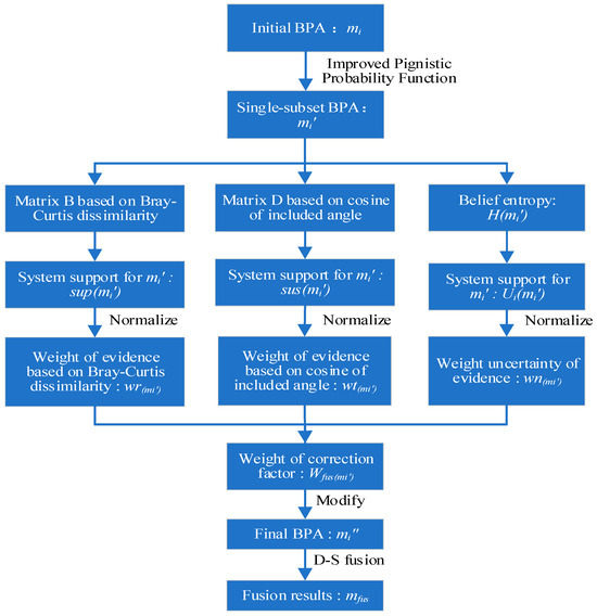
Figure 1.
The flowchart of the proposed method.
The pseudocode for the proposed method is presented in Algorithm 1, outlining the approach for weighted fusion of conflicting evidence in this paper. The final fusion result of the collected evidence can be obtained by this algorithm to support decision making.
Assume a set of original evidence sources collected within the identification framework , with the corresponding BPA function denoted as .
As depicted in Algorithm 1, lines 1–3 illustrate the process of converting collected BPA functions into a single subset of BPA functions, enhancing decision accuracy. Lines 4–12 elucidate the procedure for determining the weights of evidence similarity based on the Bray–Curtis dissimilarity. Subsequently, lines 13–21 detail the computation of evidence credibility weights using the cosine of the angle distance. Lines 22–27 articulate the methodology for assessing evidence uncertainty based on belief entropy. Further, lines 28–30 delineate the computation of the weighted fusion coefficients for evidence. Lines 31–33 expound on the correction of the original BPA function to yield the final BPA function value. Lastly, lines 34–36 explain the generation of fusion results.
| Algorithm 1 Conflict Evidence Fusion Method Based on the Bray–Curtis Dissimilarity and the Belief Entropy |
| Input: Initial BPAs: Output: Fusion Result:
|
4. Experiments
To validate the effectiveness of the conflict evidence fusion method proposed in this paper, we reference two sets of classic conflict data. The first set comprises single-subset focal element data from the literature [26], while the second set consists of multiple subset focal element data sources from the literature [7]. These two sets of data sources have been widely employed in previous studies of enhanced methods and represent two forms of BPA functions. The application of the proposed fusion method to these two conflicting datasets, along with an analytical comparison against the D-S evidence theory and various improved fusion algorithms, serves to verify the efficiency and effectiveness of the method proposed in this paper.
4.1. An Example of Single-Subset Focal Element Data
There are five pieces of evidence on the frame of discernment , and the BPA function of each evidence is as follows:
Based on intuitive analysis, evidence , , and collectively supports proposition , while evidence supports proposition with a higher degree of certainty, despite being conflicting evidence. The next step involves validation using the method proposed in this paper.
- (1)
- Improved Pignistic probability function
The mass functions in the provided examples are all single-subset focal element evidential bodies. Consequently, the mass function values after conversion through the improved Pignistic probability function remain the same as the original BPA function values. The values of converted mass function are detailed in Table 1.

Table 1.
The values of converted mass functions.
- (2)
- The Bray–Curtis dissimilarity matrix is derived from Equations (9) and (10) as follows:
Applying Equation (11), the evidence support based on the Bray–Curtis dissimilarity matrix is determined as follows:
Utilizing Equation (12) for normalization, the support coefficients become as follows:
- (3)
- Equations (13) and (14) are applied to obtain the cosine distance matrix of the included angle:
According to Equation (15), the similarity of the evidence available based on the cosine distance matrix of the included angle is determined as follows:
Normalization of the evidence similarity coefficient according to Equation (16) results in the following:
- (4)
- Applying Equations (17)–(19), the entropy of each evidence is calculated as follows:
Normalization of the evidence uncertainty coefficient according to Equation (20) yields the following:
- (5)
- According to Equations (21)–(22), the normalized evidence weighted correction coefficient is calculated as follows:
Applying Equation (23), a corresponding correction coefficient is assigned to each evidence, resulting in the final mass function value:
- (6)
- Evidence fusion is executed according to Equation (24), and the final fusion results are presented in Table 2.
Table 2. Fusion results of single-subset focal element conflict data.
- (7)
- Comparison with other improvement methods is outlined in Table 3. The variation in the mass function value of the proposition concerning different fusion rules and the number of fusions is illustrated in Figure 2.
Table 3. Fusion results of single-subset focal element conflict data under various fusion methods.
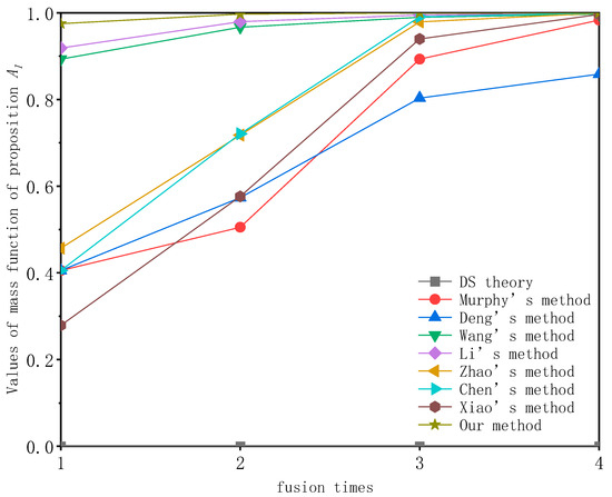 Figure 2. Mass function values of proposition for a single-subset of focal element conflict data under different fusion methods.
4.2. An Example of Multi-Subset Focal Element Data
There are five pieces of evidence on the frame of discernment , and the BPA function of each piece of evidence is, respectively, as follows:
Upon intuitive analysis, evidence , , and supports proposition , while evidence supports proposition with a higher degree of certainty, despite being conflicting evidence. Validation is performed using the proposed method.
- (1)
- Improved Pignistic probability function
For the multi-subset focal propositions , and , it is necessary to implement the improved Probabilistic transformations for their resolution.
According to Equations (3) and (4), the belief function and plausibility function values for are as follows:
According to Equations (7) and (8), the following holds:
Similarly, the following holds:
The values of mass function converted using the improved Pignistic probability function are shown in Table 4.
Table 4.
Values of mass function after being converted.
- (2)
- The Bray–Curtis dissimilarity matrix, as derived from Equations (9) and (10), is represented by the following:
Utilizing Equation (11), the support of the evidence based on the Bray–Curtis dissimilarity matrix is computed as follows:
After normalization according to Equation (12), the coefficients of support for the evidence are as follows:
- (3)
- The cosine distance matrix of the included angle, obtained from Equations (13) and (14), is given by the following:
According to Equation (15), the similarity of the evidence based on the cosine distance matrix is as follows:
The normalized evidence similarity coefficient according to Equation (16) is as follows:
- (4)
- Applying Equations (17)–(19), the entropy of each available evidence is determined as follows:
The coefficient of uncertainty of evidence after normalization according to Equation (20) is as follows:
- (5)
- According to Equations (21)–(22), the normalized evidence weighted correction coefficient is obtained as follows:
According to Equation (23), each piece of evidence is assigned a corresponding correction coefficient, and the resulting mass function value can be calculated as follows:
- (6)
- Convergence of Evidence Based on D-S Theory
Evidence fusion is carried out according to Equation (24), and the final fusion results are shown in Table 5.
Table 5.
Fusion results of multi-subset focal element conflict data.
- (7)
- Comparison with alternative improvement methods is illustrated in Table 6. The variations in the mass function value of the proposition across different fusion rules and fusion numbers are depicted in Figure 3.
Table 6. Fusion results of multi-subset focal element conflict data under different fusion methods.
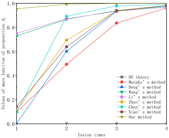 Figure 3. Change in mass function value of proposition under varying fusion rules and fusion numbers.
4.3. Discussion
In this section, we present two approaches for fusing conflicting evidence from single-subset and multi-subset focal element data sources. Initially, the effectiveness of the improved Pignistic probability function is validated. Leveraging the total likelihood of truth information from single-subset focal elements, the evidence from multi-subset focal elements is allocated to single-subset propositions based on confidence intervals. This approach maximizes the utilization of existing information, enabling the rapid identification of the correct proposition even in the presence of conflicting data sources from multi-subset focal elements.
As shown in Figure 2 and Table 3, when validating conflict data with singleton focal elements, the D-S evidence theory fails to correctly identify the proposition . Notably, the methods proposed by Xiao, Murphy, Zhao and Chen in their first fusion attempts all yielded mass function values for the proposition that did not surpass 0.5. In contrast, our proposed method achieved a substantial improvement, reaching a mass function value of 0.9751 for the proposition in the first fusion iteration, outperforming all of the aforementioned methods. With increasing fusion iterations, the mass function value for the proposition steadily increased, reaching 0.9999 in the final fusion iteration, consistently surpassing the fusion accuracy of the aforementioned improved methods. Compared to Murphy’s method, our proposed method exhibited a 1.68% improvement, a 0.36% improvement over Xiao’s method and a 0.03% improvement over Chen’s method.
As illustrated in Figure 3 and Table 6, when validating conflict data with multiple subset focal elements, the D-S evidence theory still failed to identify the correct proposition . Deng and Chen’s methods, in their initial fusion attempts, both failed to correctly identify . For Murphy, Zhao and Xiao’s methods, the mass function values for proposition did not exceed 0.2 in the first fusion iteration. In contrast, our proposed method achieved a mass function value of 0.9547 for the proposition in the first fusion iteration, reaching 0.9998 in the final fusion iteration. This consistently exceeded the fusion accuracy of the aforementioned improved methods, showing a 4% improvement over Murphy’s method, a 1.86% improvement over Xiao’s method and a 0.83% improvement over Chen’s method.
In summary, our proposed method demonstrates faster convergence and higher fusion accuracy compared to previously proposed improved methods. This validates the effectiveness and feasibility of the proposed approach.
5. Conclusions
This paper conducts a comprehensive study on conflict issues in evidence fusion, proposing the use of the improved Pignistic probability function to convert multi-subset focal element evidence into single-subset focal element evidence. This approach enhances the universality of conflict data fusion methods. The novel combination of the Bray–Curtis dissimilarity and cosine of the included angle distance is introduced as a means to measure evidence credibility. This, coupled with the belief entropy metric, gauges evidence uncertainty and determines the final weighting correction coefficients for the evidence. In the validation of conflicting evidence, the results demonstrate that the proposed method can rapidly and effectively identify target propositions. It exhibits faster convergence speed, higher fusion accuracy and better performance in addressing evidence conflict challenges.
Author Contributions
Conceptualization, Y.L.; methodology, Y.L. and T.Z.; validation, Y.L. and T.Z.; data curation, Y.L.; writing—original draft preparation, Y.L.; writing—review and editing, T.Z. and H.F. All authors have read and agreed to the published version of the manuscript.
Funding
This research received no external funding.
Data Availability Statement
No new data were created or analyzed in this study.
Conflicts of Interest
The authors declare no conflicts of interest.
References
- Dempster, A.P. Upper and Lower Probabilities Induce by a Multiplicand Mapping. Ann. Math. Stat. 1967, 38, 325–339. [Google Scholar] [CrossRef]
- Glenn, S. A Mathematical Theory of Evidence; Princeton University Press: Princeton, NJ, USA, 1976; Volume 42. [Google Scholar]
- Basir, O.; Yuan, X. Engine fault diagnosis based on multi-sensor information fusion using Dempster–Shafer evidence theory. Inf. Fusion 2007, 8, 379–386. [Google Scholar] [CrossRef]
- Zhang, X.; Ma, Y.; Li, Y.; Zhang, C.; Jia, C. Tension prediction for the scraper chain through multi-sensor information fusion based on improved Dempster-Shafer evidence theory. Alex. Eng. J. 2023, 64, 41–54. [Google Scholar] [CrossRef]
- Belmahdi, F.; Lazri, M.; Ouallouche, F.; Labadi, K.; Absi, R.; Ameur, S. Application of Dempster-Shafer theory for optimization of precipitation classification and estimation results from remote sensing data using machine learning. Remote Sens. Appl. Soc. Environ. 2023, 29, 100906. [Google Scholar] [CrossRef]
- Hamid, R.A.; Albahri, A.S.; Albahri, O.S.; Zaidan, A.A. Dempster–Shafer theory for classification and hybridised models of multi-criteria decision analysis for prioritisation: A telemedicine framework for patients with heart diseases. J. Ambient. Intell. Humaniz. Comput. 2022, 13, 4333–4367. [Google Scholar] [CrossRef]
- Chen, L.; Diao, L.; Sang, J. Weighted evidence combination rule based on evidence distance and uncertainty measure: An application in fault diagnosis. Math. Probl. Eng. 2018, 2018, 5858272. [Google Scholar] [CrossRef]
- Ghosh, N.; Saha, S.; Paul, R. iDCR: Improved Dempster Combination Rule for multisensor fault diagnosis. Eng. Appl. Artif. Intell. 2021, 104, 104369. [Google Scholar] [CrossRef]
- Fei, L.; Wang, Y. An optimization model for rescuer assignments under an uncertain environment by using Dempster–Shafer theory. Knowl.-Based Syst. 2022, 255, 109680. [Google Scholar] [CrossRef]
- Fei, L.; Feng, Y. Modeling interactive multiattribute decision-making via probabilistic linguistic term set extended by Dempster–Shafer theory. Int. J. Fuzzy Syst. 2021, 23, 599–613. [Google Scholar] [CrossRef]
- Jia, R.S.; Liu, C.; Sun, H.M.; Yan, X.H. A situation assessment method for rock burst based on multi-agent information fusion. Comput. Electr. Eng. 2015, 45, 22–32. [Google Scholar] [CrossRef]
- Liu, Z.G.; Pan, Q.; Dezert, J.; Martin, A. Adaptive imputation of missing values for incomplete pattern classification. Pattern Recognit. 2016, 52, 85–95. [Google Scholar] [CrossRef]
- Zadeh, L.A. Review of a mathematical theory of evidence. AI Mag. 1984, 5, 81. [Google Scholar]
- Cuzzolin, F. A geometric approach to the theory of evidence. IEEE Trans. Syst. ManCybern. Part C (Appl. Rev.) 2008, 38, 522–534. [Google Scholar] [CrossRef]
- Yager, R.R. On the Dempster-Shafer framework and new combination rules. Inf. Sci. 1987, 41, 93–137. [Google Scholar] [CrossRef]
- Florea, M.C.; Jousselme, A.L.; Bossé, É.; Grenier, D. Robust combination rules for evidence theory. Inf. Fusion 2009, 10, 183–197. [Google Scholar] [CrossRef]
- Su, X.; Li, L.; Qian, H.; Mahadevan, S.; Deng, Y. A new rule to combine dependent bodies of evidence. Soft Comput. 2019, 23, 9793–9799. [Google Scholar] [CrossRef]
- Murphy, C.K. Combining belief functions when evidence conflicts. Decis. Support Syst. 2000, 29, 1–9. [Google Scholar] [CrossRef]
- Yong, D.; Shi, W.; Zhu, Z.; Liu, Q. Combining belief functions based on distance of evidence. Decis. Support Syst. 2004, 38, 489–493. [Google Scholar] [CrossRef]
- Lin, Y.; Wang, C.; Ma, C.; Dou, Z.; Ma, X. A new combination method for multisensor conflict information. J. Supercomput. 2016, 72, 2874–2890. [Google Scholar] [CrossRef]
- Shi, X.; Liang, F.; Qin, P.; Yu, L.; He, G. A Novel Evidence Combination Method Based on Improved Pignistic Probability. Entropy 2023, 25, 948. [Google Scholar] [CrossRef]
- Tang, Y.; Dai, G.; Zhou, Y.; Huang, Y.; Zhou, D. Conflicting evidence fusion using a correlation coefficient-based approach in complex network. Chaos Solitons Fractals 2023, 176, 114087. [Google Scholar] [CrossRef]
- Xiao, F. Multi-sensor data fusion based on the belief divergence measure of evidences and the belief entropy. Inf. Fusion 2019, 46, 23–32. [Google Scholar] [CrossRef]
- Zhao, K.; Sun, R.; Li, L.; Hou, M.; Yuan, G.; Sun, R. An improved evidence fusion algorithm in multi-sensor systems. Appl. Intell. 2021, 51, 7614–7624. [Google Scholar] [CrossRef]
- Li, J.; Xie, B.; Jin, Y.; Hu, Z.; Zhou, L. Weighted conflict evidence combination method based on Hellinger distance and the belief entropy. IEEE Access 2020, 8, 225507–225521. [Google Scholar] [CrossRef]
- Wang, X.; Di, P.; Yin, D. Conflict evidence fusion method based on lance distance and credibility entropy. Syst. Eng. Electron. 2021, 44, 592–602. [Google Scholar] [CrossRef]
- Zhou, C.; Xu, D.; Cao, Z. Conflict evidence fusion method for single subset focus elements. J. Beijing Univ. Aeronaut. Astronaut. 2023, 1–11. [Google Scholar] [CrossRef]
- Zhang, H.; Lu, J.; Tang, X. An improved DS evidence theory algorithm for conflict evidence. J. Beijing Univ. Aeronaut. Astronaut. 2020, 46, 616–623. [Google Scholar]
- Pal, N.R.; Bezdek, J.C.; Hemasinha, R. Uncertainty measures for evidential reasoning I: A review. Int. J. Approx. Reason. 1992, 7, 165–183. [Google Scholar] [CrossRef]
- George, T.; Pal, N.R. Quantification of conflict in Dempster-Shafer framework: A new approach. Int. J. Gen. Syst. 1996, 24, 407–423. [Google Scholar] [CrossRef]
- Lefevre, E.; Colot, O.; Vannoorenberghe, P.; De Brucq, D. A generic framework for resolving the conflict in the combination of belief structures. In Proceedings of the Third International Conference on Information Fusion, Paris, France, 10–13 July 2000; IEEE: Piscataway, NJ, USA, 2000. [Google Scholar]
- Pan, W.; Wang, Y.; Yang, H. Design of Pignistic probability conversion algorithm. Comput. Eng. 2005, 31, 20–22+25. [Google Scholar]
- Dubois, D.; Prade, H. Representation and combination of uncertainty with belief functions and possibility measures. Comput. Intell. 1988, 4, 244–264. [Google Scholar] [CrossRef]
- Smets, P.; Kennes, R. The transferable belief model. Class. Work. Dempster-Shafer Theory Belief Funct. 2008, 2019, 693–736. [Google Scholar]
- Sudano, J.J. Pignistic probability transforms for mixes of low-and high-probability events. arXiv 2015, arXiv:1505.07751. [Google Scholar]
- Bray, J.R.; Curtis, J.T. An ordination of the upland forest communities of southern Wisconsin. Ecol. Monogr. 1957, 27, 326–349. [Google Scholar] [CrossRef]
- Ricotta, C.; Podani, J. On some properties of the Bray-Curtis dissimilarity and their ecological meaning. Ecol. Complex. 2017, 31, 201–205. [Google Scholar] [CrossRef]
- Ricotta, C.; Pavoine, S. A new parametric measure of functional dissimilarity: Bridging the gap between the Bray-Curtis dissimilarity and the Euclidean distance. Ecol. Model. 2022, 466, 109880. [Google Scholar] [CrossRef]
- Wen, C.; Wang, Y.; Xu, X. Fuzzy information fusion algorithm of fault diagnosis based on similarity measure of evidence. In Advances in Neural Networks-ISNN 2008, Proceedings of the 5th International Symposium on Neural Networks, ISNN 2008, Beijing, China, 24–28 September 2008; Springer: Berlin/Heidelberg, Germany, 2008; Volume 5, pp. 506–515. [Google Scholar]
- Chen, B.C.; Tao, X.; Yang, M.R.; Yu, C.; Pan, W.M.; Leung, V.C. A saliency map fusion method based on weighted DS evidence theory. IEEE Access 2018, 6, 27346–27355. [Google Scholar] [CrossRef]
- Khan, M.N.; Anwar, S. Paradox elimination in Dempster–Shafer combination rule with novel entropy function: Application in decision-level multi-sensor fusion. Sensors 2019, 19, 4810. [Google Scholar] [CrossRef]
- Shannon, C.E. A mathematical theory of communication. ACM SIGMOBILE Mob. Comput. Commun. Rev. 2001, 5, 3–55. [Google Scholar] [CrossRef]
- Deng, Y. Deng Entropy: A generalized Shannon Entropy to Measure Uncertainty. Available online: https://fs.unm.edu/DengEntropyAGeneralized.pdf (accessed on 31 January 2015).
- Yan, H.; Deng, Y. An improved belief entropy in evidence theory. IEEE Access 2020, 8, 57505–57516. [Google Scholar] [CrossRef]
- Yuan, K.; Xiao, F.; Fei, L.; Kang, B.; Deng, Y. Conflict management based on belief function entropy in sensor fusion. SpringerPlus 2016, 5, 638. [Google Scholar] [CrossRef] [PubMed]
Disclaimer/Publisher’s Note: The statements, opinions and data contained in all publications are solely those of the individual author(s) and contributor(s) and not of MDPI and/or the editor(s). MDPI and/or the editor(s) disclaim responsibility for any injury to people or property resulting from any ideas, methods, instructions or products referred to in the content. |
© 2024 by the authors. Licensee MDPI, Basel, Switzerland. This article is an open access article distributed under the terms and conditions of the Creative Commons Attribution (CC BY) license (https://creativecommons.org/licenses/by/4.0/).