Dynamical Coupling between Particle and Antiparticle in Relativistic Quantum Mechanics: A Multistate Perspective on the Energy–Momentum Relation

Abstract

A molecular formalism based on a decomposed energy space constructed by a modular basis of matter and radiation is proposed for relativistic quantum mechanics. In the proposed formalism, matter radiation interactions are incorporated via the dynamical transformation of the coupled particle/antiparticle pair in a multistate quantum mechanical framework. This picture generalizes relativistic quantum mechanics at minimal cost, unlike quantum field theories, and the relativistic energy–momentum relation is interpreted as energy transformations among different modules through a multistate Schrödinger equation. The application of two-state and four-state systems using a time-dependent Schrödinger equation with pair states as a basis leads to well-defined solutions equivalent to those obtained from the Klein–Gordon equation and the Dirac equation. In addition, the particle–antiparticle relationship is well manifested through a particle conjugation group. This work provides new insights into the underlying molecular mechanism of relativistic dynamics and the rational design of new pathways for energy transformation.

1. Introduction

The theory of quantum mechanics has achieved unprecedented success, being applied in numerous research fields spanning astronomy, physics, chemistry, and biology. Nevertheless, the understanding of some fundamental concepts in quantum mechanics is notably challenging. For example, the interpretation of the wave function and the underlying mechanism for the wave–particle duality is still under debate [1,2,3,4]. Moreover, additional puzzles appeared when quantum mechanics was generalized to a relativistic theory based on Einstein’s energy–momentum relation [5,6,7]. The resulting relativistic quantum mechanics (RQM) came out with the negative energy solution, which was interpreted as an antiparticle [5,6]. Both the particle and antiparticle can be represented by multicomponent wave functions, and they are connected through charge conjugation [8]. However, in our opinion, the underlying mathematical structure is not fully understood yet, and the particle–antiparticle interactions are obscured. Consequently, conceptual and technical difficulties arise in describing observables in relativistic dynamics, such as the position, momentum, and spin [9,10,11], and arbitrariness and inconsistencies in measurements and interpretations exist.

The research on antiparticles and antimatter has received tremendous interest [12,13,14,15,16,17], and nowadays, antiparticles and antiatoms could be produced routinely in high-energy experiments [15,16,17]. Nevertheless, the fact that the observing universe comprises matter predominately and a scarcity of antimatter [18,19,20,21] leads to a poor understanding of the properties of antimatter, and the asymmetry of matter and antimatter has not been well explained. On the other hand, in most practical applications, it is preferable to simply remove the negative energy solution. In fact, extensive efforts [22,23,24,25,26,27,28,29,30,31] have been devoted to constructing a consistent single-particle interpretation to either the Klein–Gordon equation or Dirac equation and decoupling the positive and negative energy solutions, therefore correctly nonrelativistic and semiclassical limits could be achieved, and variational collapse could be avoided. For instance, recently, the treatment of diagonalizing the Dirac Hamiltonian by using a series of unitary transformations has become successfully practical in quantum chemistry calculations (in particular) for many-electron systems [30,31]. Alternative approaches for relativistic dynamics have also been developed from a variety of perspectives [32,33,34,35,36,37,38,39,40,41,42,43]. However, the underlying mechanisms of the applied mathematical structures and transformations are often elusive.

In addition, RQM in the conventional treatments focuses on a low-energy particle picture, and matter and radiation are normally treated in different ways, whereas particle–antiparticle transformations such as pair creation and annihilation fall outside its validating regime. One may think RQM should be substituted by the more advanced modern quantum field theories (QFT) [5]. Indeed, some of the problems of RQM have been solved in QFT, but not for all [2]. However, the interpretation to wave function (or physical reality) becomes even more abstract in QFT, and the quantization of fields is performed in a predefined and parameterized space-time with infinitely many degrees of freedom. The resulting many-body picture at a higher level complicates the representation and has the disadvantage of introducing additional difficulties in understanding the underlying mechanisms of quantum mechanics.

In this work, we propose a molecular formalism for relativistic quantum mechanics based on a coherent synthesis of the mathematic framework of vector space, physical mapping of basis onto energy quanta (Planck’s particles), and chemical interpretation of energy transformation. In the proposed formalism, the energy space is decomposed into classified energy basis (modules) corresponding to matter and radiation, respectively. The modular basis can be constructed systematically and hierarchically for complicated systems in high dimensional energy space, resulting in an energy tensor (ET) representation of RQM. The ET representation of RQM incorporates matter and radiation interactions coherently as energy transformation among different energy modules and therefore goes beyond the scope of conventional RQM. In particular, the formalism geometrically illustrates a straightforward multistate interpretation of the relativistic energy–momentum relation and sheds light on the underlying molecular mechanism of relativistic dynamics and on the interpretation of dynamical variables and wave function in fundamental quantum mechanics.

In the application of this formalism on a quantum two-state model, the Hamiltonian system is projected onto energy modules in the decomposed energy space, resulting in the relativistic multistate Schrödinger equation that manifests the transformation between mass energy and radiation energy through the energy–momentum relation. For both the two-state and the extended four-state system, well-defined solutions with positive definite probability density to the equivalent Klein–Gordon equation and Dirac equation can be systematically generated, taking advantage of a universal type of unitary transformations based on a pair-state basis. This treatment simplifies the mathematical structure of the solution space and motivates us to propose a particle conjugation group to manifest the symmetry of the particle–antiparticle relationship. Although numerous unitary transformations for diagonalizing the relativistic Hamiltonian matrix [22,23,24,25,26,27,28] were developed and applied widely a long time ago, our approach is unique in its design for incorporating the dynamical coupling of matter and radiation in a unified molecular framework.

In the following, the ET formalism for relativistic quantum mechanics is proposed in Section 2, and then the solutions for both the two-state and four-state systems, equivalent to the Klein–Gordon equation and the Dirac equation, respectively, will be derived in the same molecular framework of energy space at different hierarchies. Section 3 provides discussions on energy space decomposition (ESD), energy transformation, free particle solutions, and the features of the multistate relativistic quantum mechanics in energy space. Section 4 concludes. Appendix A includes the results of comparable unitary transformations applied to RQM and the details of the solution to the four-state problem.

2. Theoretical Models

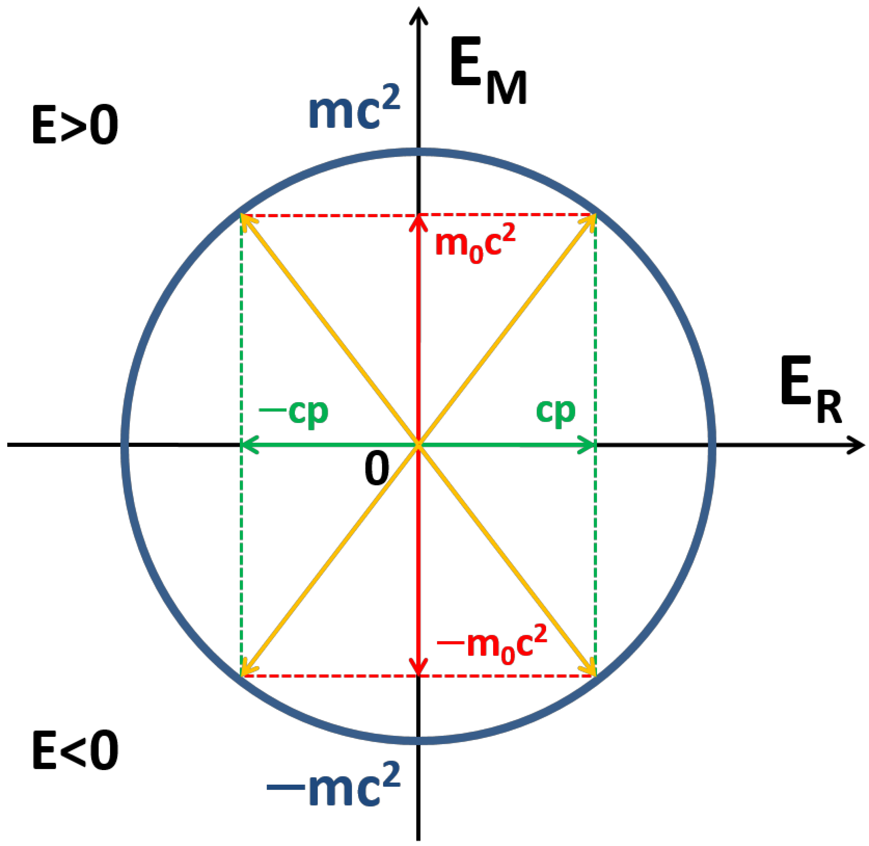
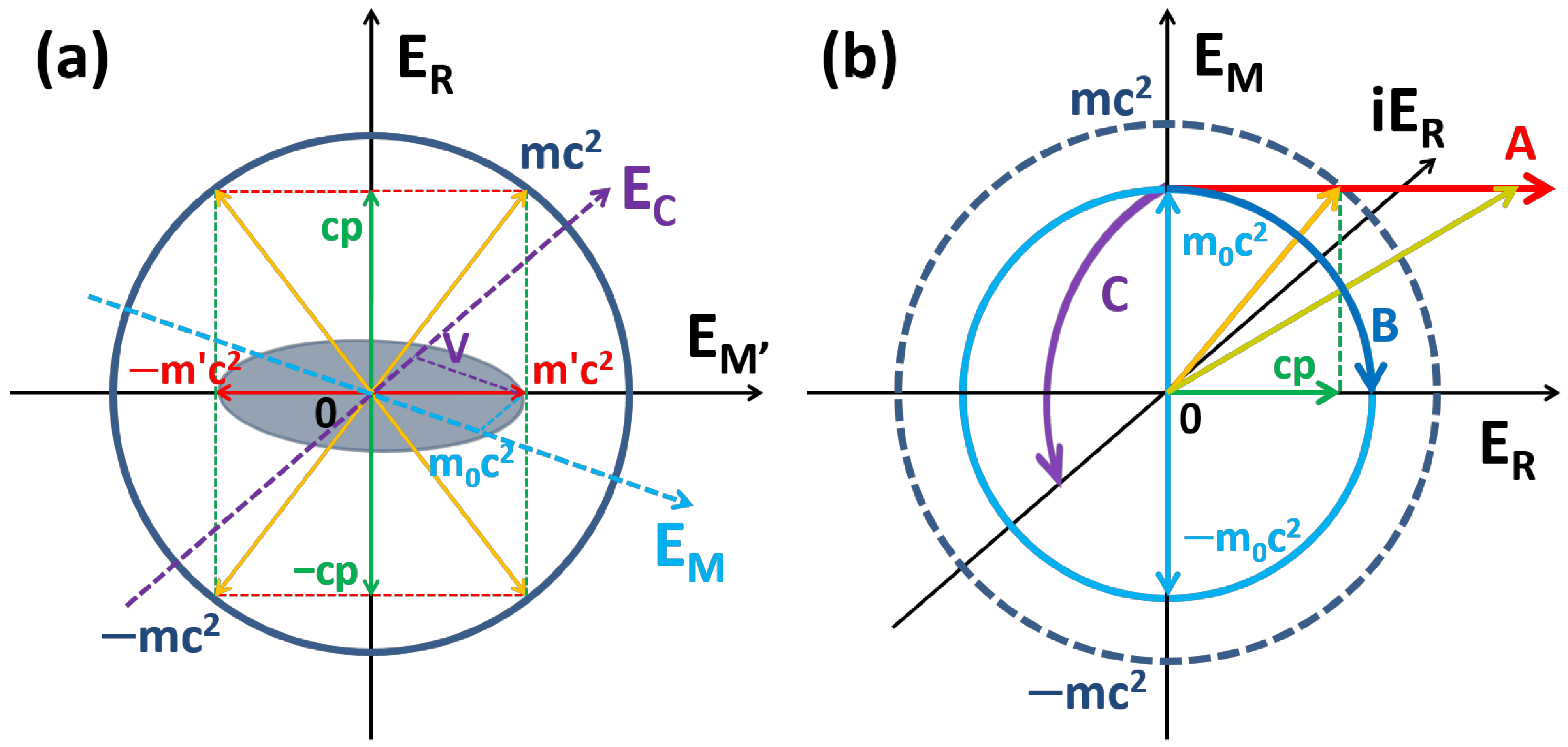
2.1. Two-State System

The quantum dynamics of an interested system, in general, may be described by the time-dependent Schrödinger equation, i.e.,

$$\mathrm{i}\hslash \frac{\partial }{\partial \mathrm{t}}|\mathsf{\psi }\rangle =\hat{\mathrm{H}}|\mathsf{\psi }\rangle$$

(1)

where $|\mathsf{\psi }\rangle$ is the ket state describing the properties of the system and the Hamiltonian operator $\hat{\mathrm{H}}$ determines the time evolution of the system. Now let us take a two-state system as an example to illustrate multistate systems in general. Instead of using the conventional coordinates space (basis), we stay with the (energy) state space and will construct the basis in this space in multidimensions. The representation of the time-dependent Schrödinger equation for this system can be written as

$$\mathrm{i}\hslash \frac{\partial }{\partial \mathrm{t}}\mathsf{\psi }=\mathrm{H}\mathsf{\psi }$$

(2a)

$$\mathrm{with} \mathsf{\psi }=\langle 1|\mathsf{\psi }\rangle \left(\begin{array}{c}1\\ 0\end{array}\right)+\langle 2|\mathsf{\psi }\rangle \left(\begin{array}{c}0\\ 1\end{array}\right)=\left(\begin{array}{c}{\mathsf{\psi }}_1\\ {\mathsf{\psi }}_2\end{array}\right), \mathrm{and}$$

(2b)

$$\mathrm{H}=\left(\begin{array}{cc}\langle 1|\hat{\mathrm{H}}|1\rangle & \langle 1|\hat{\mathrm{H}}|2\rangle \\ \langle 2|\hat{\mathrm{H}}|1\rangle & \langle 2|\hat{\mathrm{H}}|2\rangle \end{array}\right)=\left(\begin{array}{cc}{\mathrm{H}}_{11}& {\mathrm{H}}_{12}\\ {\mathrm{H}}_{21}& {\mathrm{H}}_{22}\end{array}\right)$$

(2c)

where ${\mathsf{\psi }}_{\mathrm{i}}$ is the i-th component of the state ket, ${\mathrm{H}}_{\mathrm{ij}}=\langle \mathrm{i}|\hat{\mathrm{H}}|\mathrm{j}\rangle$ is the Hamiltonian matrix element in the chosen representation, and i, j = 1, 2 are the state indexes.

The solution of Equation (2) may be found through standard treatment of an eigenvalue problem [44],

$$\left(\begin{array}{c}{\mathsf{\psi }}_1\\ {\mathsf{\psi }}_2\end{array}\right)=\mathrm{U}\left(\begin{array}{c}{\mathsf{\psi }}^{+}\\ {\mathsf{\psi }}^{-}\end{array}\right)$$

(3a)

with the corresponding eigenfunctions given by

$${\mathsf{\psi }}^{\pm }~{\mathrm{e}}^{-\frac{{\mathrm{iE}}^{\pm }\mathrm{t}}{\hslash }}$$

(3b)

and the eigenvalues of the Hamiltonian matrix being

$${\mathrm{E}}^{\pm }=\frac{1}{2}\left({\mathrm{H}}_{11}+{\mathrm{H}}_{22}\right)\pm \sqrt{\frac{{\left({\mathrm{H}}_{11}-{\mathrm{H}}_{22}\right)}^2}{4}+{\mathrm{H}}_{12}{\mathrm{H}}_{21}}$$

(3c)

The unitary transformation here effectively diagonalizes the Hamiltonian matrix and is also known as the diabatic-to-adiabatic transformation matrix.

$$U=\left(\begin{array}{cc}\cos \mathsf{\theta }& -\sin \mathsf{\theta }\\ \sin \mathsf{\theta }& \cos \mathsf{\theta }\end{array}\right)$$

(3d)

$$\mathrm{Here} \mathrm{for} \mathrm{the} \mathrm{real} \mathrm{H}, \mathsf{\theta }=\frac{1}{2}\mathrm{atan}\frac{2{\mathrm{H}}_{12}}{{\mathrm{H}}_{11}-{\mathrm{H}}_{22}}$$

(3e)

Equation (2) manifests the mathematical structure of the quantum system of interest. When mapped to physically realistic models, this simple mathematical structure could transform into a general framework to accommodate a variety of different representations in the realistic world. We start by thinking about the well-known fact of the annihilation of an electron and its antiparticle (positron) into their intermediate bosons, i.e., photons, and consider a two-state model for a particle–antiparticle pair coupled through intermediate bosons. The system Hamiltonian matrix may be represented by

$$\mathrm{H}=\left(\begin{array}{cc}{\mathrm{E}}_{\mathrm{M}}& {\mathrm{iE}}_{\mathrm{R}}\\ -{\mathrm{iE}}_{\mathrm{R}}& -{\mathrm{E}}_{\mathrm{M}}\end{array}\right)$$

(4a)

where $\mathrm{i}=\sqrt{-1}$ and the pure state energy of the particle (antiparticle) and the coupling are

$${\mathrm{E}}_{\mathrm{M}}={\mathrm{m}}_0{\mathrm{c}}^2,$$

(4b)

$${\mathrm{E}}_{\mathrm{R}}=\mathrm{pc},$$

(4c)

where ${\mathrm{m}}_0$, p, and c is the rest mass, momentum, and light speed, respectively. In this way, we effectively decompose the energy space of a multistate system into classified energy modules, namely matter and radiation (see discussion below).

Substituting the mapping scheme in Equation (4) into Equation (2) results in an explicit multistate Schrödinger Equation:

$$\mathrm{i}\hslash \frac{\partial }{\partial \mathrm{t}}\left(\begin{array}{c}{\mathsf{\psi }}_1\\ {\mathsf{\psi }}_2\end{array}\right)=\left(\begin{array}{cc}{\mathrm{m}}_0{\mathrm{c}}^2& \mathrm{icp}\\ -\mathrm{icp}& -{\mathrm{m}}_0{\mathrm{c}}^2\end{array}\right)\left(\begin{array}{c}{\mathsf{\psi }}_1\\ {\mathsf{\psi }}_2\end{array}\right)$$

(5)

The solutions to Equation (5) can be represented through Equation (3a) using the energy eigenstates,

$${\mathsf{\psi }}^{\pm }~{\mathrm{e}}^{-\frac{{\mathrm{iE}}^{\pm }\mathrm{t}}{\hslash }}$$

(6a)

$$\mathrm{with} {\mathrm{E}}^{\pm }=\pm \sqrt{{\mathrm{p}}^2{\mathrm{c}}^2+{\mathrm{m}}_0^2{\mathrm{c}}^4}=\pm {\mathrm{mc}}^2,$$

(6b)

with m being the total (renormalized) mass of the transformed particle as a composite of matter and radiation. Here we obtain the energy–momentum relation from a molecular two-state model. However, Equation (6) does not fully resolve the solution space of the multistate Schrödinger equation. An alternative way to reach another mathematically equivalent solution of Equation (5) [see Appendix A for other solutions] may adopt the following orthogonal transformation, i.e.,

$$O=\frac{1}{\sqrt{2}}\left(\begin{array}{cc}1& 1\\ 1& -1\end{array}\right)$$

(7)

So that Equation (1) becomes

$$\mathrm{i}\hslash \mathrm{O}\frac{\partial \mathsf{\psi }}{\partial \mathrm{t}}=\mathrm{OH}\tilde{\mathrm{O}}\mathrm{O}\mathsf{\psi }$$

(8a)

which is

$$\mathrm{i}\hslash \frac{\partial }{\partial \mathrm{t}}\left(\begin{array}{c}{{\mathsf{\psi }}^{\prime }}_1\\ {{\mathsf{\psi }}^{\prime }}_2\end{array}\right)=\left(\begin{array}{cc}0& {\mathrm{m}}_0{\mathrm{c}}^2-\mathrm{icp}\\ {\mathrm{m}}_0{\mathrm{c}}^2+\mathrm{icp}& 0\end{array}\right)\left(\begin{array}{c}{{\mathsf{\psi }}^{\prime }}_1\\ {{\mathsf{\psi }}^{\prime }}_2\end{array}\right)$$

(8b)

$$\mathrm{with} {\mathsf{\psi }}^{\prime }=\left(\begin{array}{c}{{\mathsf{\psi }}^{\prime }}_1\\ {{\mathsf{\psi }}^{\prime }}_2\end{array}\right)=O\left(\begin{array}{c}{\mathsf{\psi }}_1\\ {\mathsf{\psi }}_2\end{array}\right)$$

(8c)

Equation (8b) indicates that the pair state ${\mathsf{\psi }}^{\prime }$ obeys the wave equation, i.e.,

$$\frac{{\partial }^2}{\partial {\mathrm{t}}^2}{\mathsf{\psi }}^{\prime }+{\omega }^2{\mathsf{\psi }}^{\prime }=0,\; and$$

(9a)

$$\mathsf{\omega }=\frac{\mathrm{E}}{\hslash }, \mathrm{and} \mathrm{E}=\sqrt{{\mathrm{p}}^2{\mathrm{c}}^2+{\mathrm{m}}_0^2{\mathrm{c}}^4}.$$

(9b)

Therefore, we can easily write down the general form of ${\mathsf{\psi }}^{\prime }$, i.e.,

$${\mathsf{\psi }}^{\prime }=\left(\begin{array}{c}{{\mathsf{\psi }}^{\prime }}_1\\ {{\mathsf{\psi }}^{\prime }}_2\end{array}\right)=\left(\begin{array}{c}{\mathrm{Ae}}^{\mathrm{i}\mathsf{\omega }\mathrm{t}}+{\mathrm{Be}}^{-\mathrm{i}\mathsf{\omega }\mathrm{t}}\\ {\mathrm{Ce}}^{\mathrm{i}\mathsf{\omega }\mathrm{t}}+{\mathrm{De}}^{-\mathrm{i}\mathsf{\omega }\mathrm{t}}\end{array}\right).$$

(9c)

where $\mathrm{A},\mathrm{B},\mathrm{C},\mathrm{D}$ are coefficients to be determined. Substituting Equation (9c) into Equation (8b) results in linear equations of these coefficients, and the solution can be found to be

$$\begin{gathered} \mathrm{A}=\frac{-1+\mathrm{i}}{2}, \mathrm{B}=\frac{1+\mathrm{i}}{2} \\ \mathrm{C}=\frac{1}{2}\left(\frac{{\mathrm{m}}_0{\mathrm{c}}^2+\mathrm{cp}}{\mathrm{E}}-\mathrm{i}\frac{{\mathrm{m}}_0{\mathrm{c}}^2-\mathrm{cp}}{\mathrm{E}}\right) \\ \mathrm{D}=\frac{1}{2}\left(\frac{{\mathrm{m}}_0{\mathrm{c}}^2-\mathrm{cp}}{\mathrm{E}}+\mathrm{i}\frac{{\mathrm{m}}_0{\mathrm{c}}^2+\mathrm{cp}}{\mathrm{E}}\right) \end{gathered}$$

(10)

Here we allow the coefficients to be complex with the real and imaginary parts corresponding to matter and radiation, respectively. To obtain Equation (10), first A and B are chosen to reflect the fact that the pair state comprises the linear combination of particle and antiparticle states (Equation (6a)) with an equal contribution from matter and radiation, and then C and D are determined accordingly. Other equivalent forms exist. Furthermore, we find that it is illuminative to write the transformed wave function in terms of particle pair states as follows:

$${{\mathsf{\psi }}^{\prime }}_1=\frac{-1+\mathrm{i}}{2}{\mathrm{e}}^{\mathrm{i}\mathsf{\omega }\mathrm{t}}+\frac{1+\mathrm{i}}{2}{\mathrm{e}}^{-\mathrm{i}\mathsf{\omega }\mathrm{t}};$$

(11a)

$${{\mathsf{\psi }}^{\prime }}_2=\frac{{\mathrm{m}}_0{\mathrm{c}}^2+\mathrm{icp}}{\mathrm{E}}\left(\frac{1-\mathrm{i}}{2}{\mathrm{e}}^{\mathrm{i}\mathsf{\omega }\mathrm{t}}+\frac{1+\mathrm{i}}{2}{\mathrm{e}}^{-\mathrm{i}\mathsf{\omega }\mathrm{t}}\right)$$

(11b)

So the solution of Equation (5) can be written explicitly

$$\begin{gathered} {\mathsf{\psi }}_1=\frac{1}{2\sqrt{2}}\left[\left(\frac{{\mathrm{m}}_0{\mathrm{c}}^2+\mathrm{cp}-\mathrm{E}}{\mathrm{E}}-\mathrm{i}\frac{{\mathrm{m}}_0{\mathrm{c}}^2-\mathrm{cp}-\mathrm{E}}{\mathrm{E}}\right){\mathrm{e}}^{\mathrm{i}\mathsf{\omega }\mathrm{t}}+\left(\frac{{\mathrm{m}}_0{\mathrm{c}}^2-\mathrm{cp}+\mathrm{E}}{\mathrm{E}}+\mathrm{i}\frac{{\mathrm{m}}_0{\mathrm{c}}^2+\mathrm{cp}+\mathrm{E}}{\mathrm{E}}\right){\mathrm{e}}^{-\mathrm{i}\mathsf{\omega }\mathrm{t}}\right] \\ {\mathsf{\psi }}_2=\frac{1}{2\sqrt{2}}\left[\left(-\frac{{\mathrm{m}}_0{\mathrm{c}}^2+\mathrm{cp}+\mathrm{E}}{\mathrm{E}}+\mathrm{i}\frac{{\mathrm{m}}_0{\mathrm{c}}^2-\mathrm{cp}+\mathrm{E}}{\mathrm{E}}\right){\mathrm{e}}^{\mathrm{i}\mathsf{\omega }\mathrm{t}}+\left(-\frac{{\mathrm{m}}_0{\mathrm{c}}^2-\mathrm{cp}-\mathrm{E}}{\mathrm{E}}-\mathrm{i}\frac{{\mathrm{m}}_0{\mathrm{c}}^2+\mathrm{cp}-\mathrm{E}}{\mathrm{E}}\right){\mathrm{e}}^{-\mathrm{i}\mathsf{\omega }\mathrm{t}}\right] \end{gathered}$$

(12)

The positive and negative energy solutions to relativistic equations were conventionally interpreted as the wave functions of the particle and antiparticle, respectively, which are connected to each other under charge conjugation [8]. However, this charge conjugation is not a symmetry transformation of the relativistic dynamics [5]. Furthermore, it is not represented in a universal form indicating that the underlying mathematical structure is obscured. For example, the charge conjugation transform takes different forms for the Klein–Gordon equation and the Dirac equation [5].

Here we suggest an alternative connection between particles and antiparticles via energy conjugation. The energy conjugation is defined by a symmetry transformation in the energy space, i.e.,

$$\mathbb{E}|\mathsf{\Psi }\rangle =|\overline{\mathsf{\Psi }}\rangle , \mathbb{E}|\overline{\mathsf{\Psi }}\rangle =|\mathsf{\Psi }\rangle ;$$

(13a)

where $|\mathsf{\Psi }\rangle$ and $|\overline{\mathsf{\Psi }}\rangle$ are the quantum states of the system corresponding to the particle and antiparticle, respectively. It is clear that the identity transformation $I={\mathbb{E}}^2$ and the group of $\left\{I, \mathbb{E}\right\}$ are isomorphic to the space inversion group.

In the case of the simple two-state system, the energy space representation of energy conjugation is $\mathbb{E}=\left(\begin{array}{cc}0& 1\\ 1& 0\end{array}\right)$, and we have $\mathbb{E}\mathrm{H}{\mathbb{E}}^{-1}=-\mathrm{H}$. The result of the transformation is the sign flip of the Hamiltonian matrix, or all the matrix elements associated with classified energy modules. Consistently, the two components of the solution in Equation (12) are interchangeable with each other when both the signs of the matter module and the radiation module are reversed, or when the sign of the total energy E is reversed. Therefore, we may associate these two components with the particle and antiparticle states, respectively. This picture is clearly different from the conventional multicomponent representation of the particle (antiparticle) state (see discussion below). Therefore, the energy conjugation here and the conventional charge conjugation are two different representations of the particle–antiparticle relationship.

In the same spirit to introduce energy conjugation, we may define two closely related conjugation relationships, i.e., matter conjugation and radiation conjugation. The matter conjugation may be defined by

$$\mathbb{M}|\mathsf{\Psi }\rangle =-|\mathsf{\Psi }{\rangle }^{*}.$$

(13b)

Therefore, radiation conjugation can be represented by

$$ℝ=\mathbb{M}\mathbb{E}.$$

(13c)

For the two-state system given in Equation (5), it is easy to see that the matter conjugation of the particle (and antiparticle) state (Equation (12)) satisfies that:

$$\mathbb{M}|\mathsf{\Psi }\left({\mathrm{m}}_0\right)\rangle =-|\mathsf{\Psi }{\rangle }^{*}=|\mathsf{\Psi }\left(-{\mathrm{m}}_0\right)\rangle .$$

(13d)

Here matter and antimatter can be interpreted as mirror images of each other under the matter conjugation transformation. Therefore, $\mathbb{M}$ and the identity transformation I form a symmetric group in the energy space isomorphic to $Z_2$ or the reflection group. Similarly, the radiation conjugation may be represented by the sign flip of the radiation module, i.e.,

$$ℝ|\mathsf{\Psi }\left(\mathrm{p}\right)\rangle =|\mathsf{\Psi }\left(-\mathrm{p}\right)\rangle .$$

(13e)

Thus, it can be associated with a two-fold symmetry axis, or a reflection with respect to the matter plane. Altogether, these three types of conjugation ($\mathbb{E}, \mathbb{M}, \mathrm{and} \mathbb{R}$) and the identity transformation I constitute a group of particle conjugation isomorphic to the vierergruppe V₄.

The symmetry captured by the particle conjugation group is illustrated in Figure 1. It shows that the energy eigenstates, i.e., particle and antiparticle, can be represented by matter modules (matter and antimatter) or radiation modules (intermediate bosons), or a combination of both, as indicated in Equations (5) and (6). In addition, the mathematical structure of the energy space indicates that the system may also transform from matter modules into radiation modules or vice versa under unitary transformations. Moreover, there is no need to worry about requiring the energy bounded from below since the sign and the direction of energy (tensor) only manifest the types of various energy modules and do not count when only the magnitude of the energy is concerned. Physically, the coupling of matter (or antimatter) and radiation would not change the polarization of the renormalized matter state (or the sign of the energy of the particle/antiparticle). Specifically, all state transitions for a particle (m > 0) would stay in the upper plane in the energy space (Figure 1). The transition from positive energy levels to negative energy levels has to involve the crossing between different systems (i.e., particle and antiparticle), which requires at least an extra energy of $2E_M$.

It would be interesting to examine some features of the relativistic multistate Schrödinger Equation in the matrix form, i.e., Equation (5). It transforms into the Klein–Gordon (KG) equation for a spin zero system upon the diagonalization of the state space, i.e.,

$$-{\hslash }^2\frac{{\partial }^2{\mathsf{\psi }}_D}{\partial {\mathrm{t}}^2}={\mathrm{E}}^2{\mathsf{\psi }}_D=\left({\mathrm{p}}^2{\mathrm{c}}^2+{\mathrm{m}}_0^2{\mathrm{c}}^4\right){\mathsf{\psi }}_D$$

(14)

Indeed, the same equation can also be obtained (see Equation (9)) provided the state space can be decomposed into the two disjointed subspaces with certain mapping schemes. Some limiting cases are worth noting. First, for the strong coupling case when $\mathrm{cp}\gg {\mathrm{m}}_0{\mathrm{c}}^2$, we have

$$\mathrm{i}\hslash \frac{\partial }{\partial \mathrm{t}}\left(\begin{array}{c}{\mathsf{\psi }}_1\\ {\mathsf{\psi }}_2\end{array}\right)\approx \left(\begin{array}{cc}0& \mathrm{icp}\\ -\mathrm{icp}& 0\end{array}\right)\left(\begin{array}{c}{\mathsf{\psi }}_1\\ {\mathsf{\psi }}_2\end{array}\right)$$

(15)

In fact, when ${\mathrm{m}}_0=0, \mathrm{E}=\mathrm{cp}$, Equation (14) is reduced to a conventional wave equation for radiation such as a photon, i.e.,

$$\frac{{\partial }^2\mathsf{\psi }}{\partial {\mathrm{t}}^2}=-{\left(\frac{\mathrm{pc}}{\hslash }\right)}^2\mathsf{\psi }=-{\mathsf{\omega }}^2\mathsf{\psi }$$

(16)

Consistently, the solution (Equation (12)) gives the particle/antiparticle in radiation states (particle state in the radiation limit):

$${\mathsf{\psi }}_1=\frac{1}{\sqrt{2}}\mathrm{i}\left({\mathrm{e}}^{\mathrm{i}\mathsf{\omega }\mathrm{t}}+{\mathrm{e}}^{-\mathrm{i}\mathsf{\omega }\mathrm{t}}\right); {\mathsf{\psi }}_2=-\frac{1}{\sqrt{2}}\left({\mathrm{e}}^{\mathrm{i}\mathsf{\omega }\mathrm{t}}-{\mathrm{e}}^{-\mathrm{i}\mathsf{\omega }\mathrm{t}}\right).$$

(17a)

The corresponding particle pair states are

$${{\mathsf{\psi }}^{\prime }}_1=\frac{-1+\mathrm{i}}{2}{\mathrm{e}}^{\mathrm{i}\mathsf{\omega }\mathrm{t}}+\frac{1+\mathrm{i}}{2}{\mathrm{e}}^{-\mathrm{i}\mathsf{\omega }\mathrm{t}}; {{\mathsf{\psi }}^{\prime }}_2=\frac{1+\mathrm{i}}{2}{\mathrm{e}}^{\mathrm{i}\mathsf{\omega }\mathrm{t}}+\frac{-1+\mathrm{i}}{2}{\mathrm{e}}^{-\mathrm{i}\mathsf{\omega }\mathrm{t}}.$$

(17b)

Note that both sets of wave functions in Equation (17) are radiation-like. Here the energy eigenstates of the system (Equation (6a)) are the linear combination (coherent mixture) of the radiation states, i.e., both are connected through a unitary transformation,

$$\left(\begin{array}{c}{\mathsf{\psi }}^{+}\\ {\mathsf{\psi }}^{-}\end{array}\right)=\mathrm{L}\left(\begin{array}{c}{\mathsf{\psi }}_1\\ {\mathsf{\psi }}_2\end{array}\right)=\frac{1}{\sqrt{2}}\left(\begin{array}{c}-{\mathrm{i}\mathsf{\psi }}_1+{\mathsf{\psi }}_2\\ -{\mathrm{i}\mathsf{\psi }}_1-{\mathsf{\psi }}_2\end{array}\right)$$

(18)

On the other hand, when $\mathrm{cp}\to 0$, Equation (6) reaches the weak coupling case, i.e.,

$$\mathrm{i}\hslash \frac{\partial }{\partial \mathrm{t}}\left(\begin{array}{c}{\mathsf{\psi }}_1\\ {\mathsf{\psi }}_2\end{array}\right)\approx \left(\begin{array}{cc}{\mathrm{m}}_0{\mathrm{c}}^2& 0\\ 0& -{\mathrm{m}}_0{\mathrm{c}}^2\end{array}\right)\left(\begin{array}{c}{\mathsf{\psi }}_1\\ {\mathsf{\psi }}_2\end{array}\right)$$

(19)

The particle (and antiparticle) state can be approximated by

$$\mathrm{i}\hslash \frac{\partial }{\partial \mathrm{t}}{\mathsf{\psi }}^{+}={\mathrm{E}}^{+}{\mathsf{\psi }}^{+}\approx \left({\mathrm{m}}_0{\mathrm{c}}^2+\frac{{\mathrm{p}}^2}{2{\mathrm{m}}_0}-\dots \right){\mathsf{\psi }}^{+}$$

(20a)

$$\mathrm{i}\hslash \frac{\partial }{\partial \mathrm{t}}{\mathsf{\psi }}^{-}={\mathrm{E}}^{-}{\mathsf{\psi }}^{-}\approx -\left({\mathrm{m}}_0{\mathrm{c}}^2+\frac{{\mathrm{p}}^2}{2{\mathrm{m}}_0}-\dots \right){\mathsf{\psi }}^{-}$$

(20b)

If we transform to the operator form and leave out the highly oscillatory term due to the energy ${\mathrm{m}}_0{\mathrm{c}}^2$, Equations (20a) and (20b) are reduced to the standard nonrelativistic Schrödinger equation for a single free particle (antiparticle), i.e.,

$$\hslash \frac{\partial \mathsf{\psi }}{\partial \mathrm{t}}=-\frac{{\hslash }^2}{2\left(\pm {\mathrm{m}}_0\right)}{\nabla }^2\mathsf{\psi }.$$

(21)

In particular, when $\mathrm{p}=0, \mathrm{E}={\mathrm{m}}_0{\mathrm{c}}^2$, the particle and antiparticle states read

$${\mathsf{\psi }}_1=\frac{1}{\sqrt{2}}\left(1+\mathrm{i}\right){\mathrm{e}}^{-\mathrm{i}\mathsf{\omega }\mathrm{t}}; {\mathsf{\psi }}_2=\frac{1}{\sqrt{2}}\left(-1+\mathrm{i}\right){\mathrm{e}}^{\mathrm{i}\mathsf{\omega }\mathrm{t}}.$$

(22a)

They are matter states (particle state in the matter limit) represented by completely decoupled energy eigenstates, i.e., ${\mathsf{\psi }}^{+}\to {\mathsf{\psi }}_1$, and ${\mathsf{\psi }}^{-}\to {\mathsf{\psi }}_2$. Interestingly, the corresponding particle pair states are

$${{\mathsf{\psi }}^{\prime }}_1=\frac{-1+\mathrm{i}}{2}{\mathrm{e}}^{\mathrm{i}\mathsf{\omega }\mathrm{t}}+\frac{1+\mathrm{i}}{2}{\mathrm{e}}^{-\mathrm{i}\mathsf{\omega }\mathrm{t}}; {{\mathsf{\psi }}^{\prime }}_2=\frac{1-\mathrm{i}}{2}{\mathrm{e}}^{\mathrm{i}\mathsf{\omega }\mathrm{t}}+\frac{1+\mathrm{i}}{2}{\mathrm{e}}^{-\mathrm{i}\mathsf{\omega }\mathrm{t}}.$$

(22b)

Here we obtain one matter-like wave function and another radiation-like function, in contrast to the radiation limiting case in Equation (17). Note that when radiation particles form the pair state, the polarization changes from linear to circular, which may facilitate the matter radiation transformation.

To illustrate the difference between the above two limiting cases, we consider the parity of the wave functions under the matter conjugation. Therefore, for the matter state, we have $\mathbb{M}{\psi }_1={\psi }_2 \mathrm{and} \mathbb{M}{\psi }_2={\psi }_1$; and for the pair states, $\mathbb{M}{{\psi }^{\prime }}_1={{\psi }^{\prime }}_1 \mathrm{and} \mathbb{M}{{\psi }^{\prime }}_2=-{{\psi }^{\prime }}_2$. In contrast, for the radiation state, we obtain $\mathbb{M}{\psi }_1={\psi }_1 \mathrm{and} \mathbb{M}{\psi }_2={\psi }_2$; and for the pair states, $\mathbb{M}{{\psi }^{\prime }}_1={{\psi }^{\prime }}_1 \mathrm{and} \mathbb{M}{{\psi }^{\prime }}_2={{\psi }^{\prime }}_2$. In the former case, one of the two pair states has odd parity and the other has even parity, while in the latter case, both pair states have even parity under matter conjugation. All these observations are consistent with the result of matter conjugation as a reflection transformation.

The probability density and flux probability are also well-defined in the two-state model. According to Equation (5), we have [1]

$$\mathrm{i}\hslash {\mathsf{\psi }}_1^{*}\frac{\partial {\mathsf{\psi }}_1}{\partial \mathrm{t}}={\mathsf{\psi }}_1^{*}{\mathrm{H}}_{11}{\mathsf{\psi }}_1+{\mathsf{\psi }}_1^{*}{\mathrm{H}}_{12}{\mathsf{\psi }}_2$$

(23a)

$$-\mathrm{i}\hslash {\mathsf{\psi }}_1\frac{\partial {\mathsf{\psi }}_1^{*}}{\partial \mathrm{t}}={\mathsf{\psi }}_1{\mathrm{H}}_{11}{\mathsf{\psi }}_1^{*}+{\mathsf{\psi }}_1{\mathrm{H}}_{12}^{*}{\mathsf{\psi }}_2^{*}.$$

(23b)

Subtracting Equation (23b) from (23a), we obtain

$$\mathrm{i}\hslash \frac{\partial {\left|{\mathsf{\psi }}_1\right|}^2}{\partial \mathrm{t}}={\mathsf{\psi }}_1^{*}{\mathrm{H}}_{12}{\mathsf{\psi }}_2-{\mathsf{\psi }}_1{\mathrm{H}}_{12}^{*}{\mathsf{\psi }}_2^{*}$$

(24a)

If we write the momentum in the operator form, this equation becomes

$$\frac{\partial {\mathsf{\rho }}_1}{\partial \mathrm{t}}=-\mathrm{ic}\left({\mathsf{\psi }}_1^{*}\nabla {\mathsf{\psi }}_2-{\mathsf{\psi }}_1\nabla {\mathsf{\psi }}_2^{*}\right),$$

(24b)

where ${\mathsf{\rho }}_1={\left|{\mathsf{\psi }}_1\right|}^2$. If we consider the other component in Equation (5) based on a steady-state approximation of that ${\mathsf{\psi }}_2=-\frac{\hslash \nabla }{{\mathrm{m}}_0\mathrm{c}}{\mathsf{\psi }}_1$, Equation (24b) can be written as

$$\frac{\partial {\mathsf{\rho }}_1}{\partial \mathrm{t}}=-2\nabla {\mathrm{J}}_1, \mathrm{with} {\mathrm{J}}_1=-\frac{\mathrm{i}\hslash }{2{\mathrm{m}}_0}\left({\mathsf{\psi }}_1^{*}\nabla {\mathsf{\psi }}_1-{\mathsf{\psi }}_1\nabla {\mathsf{\psi }}_1^{*}\right)$$

(24c)

Similarly, for state 2, we have

$$\frac{\partial {\mathsf{\rho }}_2}{\partial \mathrm{t}}=-2\nabla {\mathrm{J}}_2, \mathrm{with} {\mathrm{J}}_2=-\frac{\mathrm{i}\hslash }{2\left(-\right){\mathrm{m}}_0}\left({\mathsf{\psi }}_2^{*}\nabla {\mathsf{\psi }}_2-{\mathsf{\psi }}_2\nabla {\mathsf{\psi }}_2^{*}\right).$$

(24d)

Equation (24b–d) indicates that the change in the probability density is simply due to the interstate transfer. The change in the normalized total probability density is given by

$$\frac{\partial \mathsf{\rho }}{\partial \mathrm{t}}=\frac{1}{2}\left(\frac{\partial {\mathsf{\rho }}_1}{\partial \mathrm{t}}+\frac{\partial {\mathsf{\rho }}_2}{\partial \mathrm{t}}\right)=-\left(\nabla {\mathrm{J}}_1+\nabla {\mathrm{J}}_2\right)=-\nabla \mathrm{J}.$$

(25)

Now we obtain the continuity equation with positive definite probability densities.

For the solution to the two-state model given in Equation (12), the state population of the two states is:

$$\begin{gathered} {\left|{\mathsf{\psi }}_1\right|}^2=1+\frac{\mathrm{cp}}{\mathrm{E}}cos2\omega t \\ {\left|{\mathsf{\psi }}_2\right|}^2=1-\frac{\mathrm{cp}}{\mathrm{E}}cos2\omega t. \end{gathered}$$

(26)

Here, the role of intermediate bosons is clearly demonstrated through the time-dependent term. In other words, particles and antiparticles are coupled with each other through intermediate bosons (radiation) dynamically. Moreover, it can be verified that the continuity equation, Equation (25), is satisfied.

Although the energy–momentum relation in the theory of relativity connects mass with energy, no clue was provided about how exactly energy transformation occurs. Here the relativistic multistate Schrödinger equation suggests a molecular interpretation of the energy–momentum relation via dynamical coupling and transition between particle and antiparticle and a geometric relation in the energy space mapped to the energy decomposition into different types of energy modules (Figure 1). Our analysis further shows that the first-order (with respect to time) single-particle Schrödinger equation (good for the matter-like case) and the second-order (with respect to time) Klein–Gordon equation (good for the radiation-like case) can be connected through dynamical coupling of matter and radiation in the unified ESD framework. To our knowledge, this is the first time that such a transformation between mass energy and radiation energy is manifested clearly in a molecular model. In addition, the projection of the particle (antiparticle) state onto the matter and radiation basis straightforwardly illustrates the wave–particle (matter) duality. Note that our model assumes that a pure matter state (and pure radiation state) exists, which possesses a pure corpuscular/particle (or pure wave) characteristic (detailed classification of energy modules to be presented in separate work). Also, Figure 1 is like a phase diagram consisting of only equilibrium/stationary states of the system, while the realistic (nonequilibrium/nonstationary) dynamics may be much richer and more complicated.

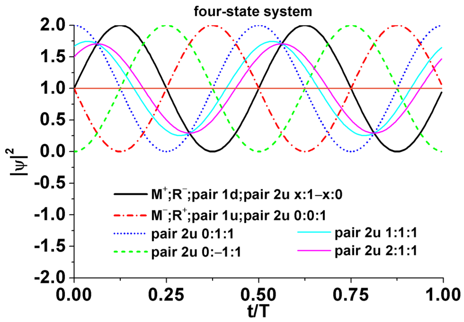
2.2. Four-State System

When the state space expands to a higher hierarchy to incorporate an extra spin degree of freedom, the treatment of the relativistic spin-1/2 particle follows the same pattern as that for the two-state system. The resulting relativistic multistate Schrödinger equation (essentially the Dirac equation) reads:

$$\mathrm{i}\hslash \frac{\partial }{\partial \mathrm{t}}\left(\begin{array}{c}{\mathsf{\psi }}_1\\ {\mathsf{\psi }}_2\end{array}\right)=\left(\begin{array}{cc}I{\mathrm{m}}_0{\mathrm{c}}^2& i\sigma \cdot \mathrm{c}p\\ -i\sigma \cdot \mathrm{c}p& -I{\mathrm{m}}_0{\mathrm{c}}^2\end{array}\right)\left(\begin{array}{c}{\mathsf{\psi }}_1\\ {\mathsf{\psi }}_2\end{array}\right),$$

(27a)

$$\mathrm{with} {\mathsf{\psi }}_{\mathrm{i}}=\left(\begin{array}{c}{\mathsf{\psi }}_{\mathrm{i}}^{\mathrm{u}}\\ {\mathsf{\psi }}_{\mathrm{i}}^{\mathrm{d}}\end{array}\right) , \mathrm{i}=1,2$$

(27b)

and each i-th wave function now comprises the up and down components, i.e., ${\mathsf{\psi }}_{\mathrm{i}}^{\mathrm{u}}$ and ${\mathsf{\psi }}_{\mathrm{i}}^{\mathrm{d}}$. The Hamiltonian matrix elements become 2 × 2 matrices, i.e.,

$$\mathrm{H}=\left(\begin{array}{cc}I{\mathrm{H}}_{11}& \sigma \cdot {\mathrm{H}}_{12}\\ \sigma \cdot {\mathrm{H}}_{21}& I{\mathrm{H}}_{22}\end{array}\right).$$

(27c)

in terms of the unit matrix $I=\left(\begin{array}{cc}1& 0\\ 0& 1\end{array}\right)$, and the Pauli matrices $\sigma =\left({\mathsf{\sigma }}_1,{\mathsf{\sigma }}_2,{\mathsf{\sigma }}_3\right)$, ${\mathsf{\sigma }}_1=\left(\begin{array}{cc}0& 1\\ 1& 0\end{array}\right)$, ${\mathsf{\sigma }}_2=\left(\begin{array}{cc}0& -\mathrm{i}\\ \mathrm{i}& 0\end{array}\right)$, ${\mathsf{\sigma }}_3=\left(\begin{array}{cc}1& 0\\ 0& -1\end{array}\right)$. Equation (27) can also transform into the Klein–Gordon-like equation under the unitary transformation similar to Equation (7), i.e.,

$$-{\hslash }^2\frac{{\partial }^2\mathsf{\psi }}{\partial {\mathrm{t}}^2}={\mathrm{E}}^2\mathsf{\psi }=\left({\mathrm{p}}^2{\mathrm{c}}^2+{\mathrm{m}}_0^2{\mathrm{c}}^4\right)\mathsf{\psi }.$$

(28)

The eigenvalues of the Hamiltonian are the same as that of the two-state system (Equation (6b)), each of which is now doubly degenerated corresponding to two spin components. The positive and negative solutions to Equation (27) (see the Appendix A) are images symmetrical to each other under the energy conjugation (Equation (13a)).

Similar to the two-state case, a straightforward calculation leads to the transformed wave function of particle pair states:

$${{\psi }^{\prime }}_1^u={\chi }_R^{+};$$

(29a)

$${{\psi }^{\prime }}_2^u=\frac{{\mathrm{m}}_0{\mathrm{c}}^2+{\mathrm{icp}}_{\mathrm{z}}}{\mathrm{E}}{\chi }_M^{+}+\frac{\mathrm{i}\left({\mathrm{cp}}_{\mathrm{x}}-{\mathrm{kcp}}_{\mathrm{y}}\right)}{\mathrm{E}}{\chi }_M^{-};$$

(29b)

$${{\psi }^{\prime }}_1^d=-{\chi }_R^{-};$$

(29c)

$${{\psi }^{\prime }}_2^d=\frac{{\mathrm{m}}_0{\mathrm{c}}^2-{\mathrm{icp}}_{\mathrm{z}}}{\mathrm{E}}{\chi }_M^{-}+\frac{\mathrm{i}\left({\mathrm{cp}}_{\mathrm{x}}+{\mathrm{kcp}}_{\mathrm{y}}\right)}{\mathrm{E}}{\chi }_M^{+},$$

(29d)

where ${\mathrm{p}}_{\mathrm{x}},{\mathrm{p}}_{\mathrm{y}},{\mathrm{p}}_{\mathrm{z}}$ are components of the momentum projecting on the x, y, and z axis in the three-dimensional space. Here a new set of (modular) composite bases is constructed based on the eigenstates in Equation (6) with positive and negative frequencies (Figure 2a), which provides an alternative decomposition scheme for the energy space, i.e.,

$${\chi }_M^{+}=\frac{1-\mathrm{i}}{2}{\mathsf{\varphi }}_{-}+\frac{1+\mathrm{i}}{2}{\mathsf{\varphi }}_{+};$$

(30a)

$${\chi }_M^{-}=\frac{1+\mathrm{i}}{2}{\mathsf{\varphi }}_{-}+\frac{1-\mathrm{i}}{2}{\mathsf{\varphi }}_{+};$$

(30b)

$${\chi }_R^{+}=\mathrm{i}{\chi }_M^{-};$$

(30c)

$${\chi }_R^{-}=\mathrm{i}{\chi }_M^{+};$$

(30d)

$$\mathrm{with} {\mathsf{\varphi }}_{\pm }={\mathrm{e}}^{\mp \mathrm{i}\mathsf{\omega }\mathrm{t}}.$$

(30e)

Figure 2b–e schematically displays the pair states in Equation (29) represented in this four-dimensional modular basis, i.e., Equation (30).

Some limiting cases are worth noting for the wave functions in Equation (29). For massless particles, i.e., ${\mathrm{m}}_0=0, \mathrm{E}=\mathrm{cp}$, the wave functions of the pair states are

$${{\psi }^{\prime }}_1^u={\chi }_R^{+}; {{\psi }^{\prime }}_1^d=-{\chi }_R^{-};$$

(31a)

$${{\psi }^{\prime }}_2^u={\chi }_R^{-}; {{\psi }^{\prime }}_2^d=-{\chi }_R^{+}.$$

(31b)

The corresponding particles (and antiparticle) read:

$$\begin{gathered} {\psi }_1^u=\frac{1}{\sqrt{2}}\mathrm{i}\left({\mathsf{\varphi }}_{-}+{\mathsf{\varphi }}_{+}\right)=\frac{1}{\sqrt{2}}\left({\chi }_R^{+}+{\chi }_R^{-}\right); \\ {\psi }_1^d=-\frac{1}{\sqrt{2}}\mathrm{i}\left({\mathsf{\varphi }}_{-}+{\mathsf{\varphi }}_{+}\right)=-\frac{1}{\sqrt{2}}\left({\chi }_R^{-}+{\chi }_R^{+}\right); \\ {\psi }_2^u=\frac{1}{\sqrt{2}}\left({\mathsf{\varphi }}_{+}-{\mathsf{\varphi }}_{-}\right)=\frac{1}{\sqrt{2}}\left({\chi }_R^{+}-{\chi }_R^{-}\right); \\ {\psi }_2^d=\frac{1}{\sqrt{2}}\left({\mathsf{\varphi }}_{+}-{\mathsf{\varphi }}_{-}\right)=\frac{1}{\sqrt{2}}\left({\chi }_R^{+}-{\chi }_R^{-}\right). \end{gathered}$$

(32)

In contrast, when $\mathrm{p}=0, \mathrm{E}={\mathrm{m}}_0{\mathrm{c}}^2$, the particle/antiparticle states become

$$\begin{gathered} {\psi }_1^u=\frac{1}{\sqrt{2}}\left(1+\mathrm{i}\right){\mathrm{e}}^{-\mathrm{i}\mathsf{\omega }\mathrm{t}}; {\psi }_1^d=\frac{1}{\sqrt{2}}\left(1-\mathrm{i}\right){\mathrm{e}}^{-\mathrm{i}\mathsf{\omega }\mathrm{t}}; \\ {\psi }_2^u=-\frac{1}{\sqrt{2}}\left(1-\mathrm{i}\right){\mathrm{e}}^{\mathrm{i}\mathsf{\omega }\mathrm{t}}; {\psi }_2^d=-\frac{1}{\sqrt{2}}\left(1+\mathrm{i}\right){\mathrm{e}}^{\mathrm{i}\mathsf{\omega }\mathrm{t}}. \end{gathered}$$

(33)

Here, all four types of composite basis survive as particle pair states, i.e.,

$$\begin{gathered} {{\psi }^{\prime }}_1^u={\chi }_R^{+}; {{\psi }^{\prime }}_1^d=-{\chi }_R^{-}; \\ {{\psi }^{\prime }}_2^u={\chi }_M^{+}; {{\psi }^{\prime }}_2^d={\chi }_M^{-}. \end{gathered}$$

(34)

Equations (32)–(34) clearly indicate that Equation (29) gives only one independent pair of massless particle/antiparticle, but two pairs of massive particles. It also shows that the massive particles/antiparticles comprise both matter and radiation components while the massless particles/antiparticles are made of radiation components only. Consistently, the moduli of the component of the total wave function (see Appendix A) are all constantly unity for the former case but all vary dramatically for the latter case, and there exists energy flux between the two component pairs of the wave function ${\psi }_1^u/{\psi }_2^u$ and ${\psi }_1^d/{\psi }_2^d$.

The parity of the wave functions under the matter conjugation is similar to that for the two-state problem. For the matter state, the two states are matter conjugated with each other, i.e.,$\mathbb{M}{\psi }_1={\psi }_2 \mathrm{and} \mathbb{M}{\psi }_2={\psi }_1$, for both up and down components. In contrast, radiation states are invariant under matter conjugation, i.e., $\mathbb{M}{\psi }_1={\psi }_1 \mathrm{and} \mathbb{M}{\psi }_2={\psi }_2$. In the former case, one pair state (${\chi }_M^{\pm }$) has odd parity and the other (${\chi }_R^{\pm }$) has even parity, while all have even parity under matter conjugation in the latter case.

These observations seem consistent with the fact that the annihilation of electrons and positrons results in photons, which have only two degrees of freedom (DOFs) and the extra DOFs are normally disregarded by applying gauge constraints. Here it implies that the extra DOFs may be associated with another massless neutral pair (MLNP), so that the dimensionality of the state space is conserved (see further discussions below).

3. Discussions

3.1. ESD and Energy Transformation

What is the motivation for the proposed energy space decomposition and the mathematical mapping suggested by Equation (4)? What are the underlying mechanisms of this framework? We know that in quantum mechanics, a system of interest can be described in general by a state (or wave function) in terms of a complete basis set in vector space. The basis is normally constructed from the eigenstates of some specific operators associated with particular physical observables of the interested system (e.g., energy eigenstates). Moreover, different bases could result in different representations of the system from different perspectives. Here we suggest using a generalized energy space to quantify the system of interest. Rather than just using the traditional (scalar) energy eigenstates of the Hamiltonian system, materializing the mathematical basis or the classification of the energy eigenstates is investigated to explore the detailed structure of the energy space, and to better understand the properties of the system.

To elaborate on our idea, let us take a simple two-state model as an example [44], i.e.,

$$\begin{array}{l}{\mathrm{H}}_0={\mathrm{E}}_{\mathrm{M}}|1\rangle \langle 1|-{\mathrm{E}}_{\mathrm{M}}|2\rangle \langle 2|;\\ \mathrm{V}\left(\mathrm{t}\right)={\mathrm{Ve}}^{-\mathrm{i}{\mathsf{\omega }}^{\prime }\mathrm{t}}|1\rangle \langle 2|+{\mathrm{Ve}}^{\mathrm{i}{\mathsf{\omega }}^{\prime }\mathrm{t}}|2\rangle \langle 1|\end{array}.$$

(35a)

Here the diagonal elements represent the eigenstates of the system Hamiltonian matrix when there are no interactions between the two states. The off-diagonal elements represent the interstate interactions described by a time-dependent potential. The solution to this problem is well known as the Rabi oscillation with a frequency of

$$\begin{gathered} \hslash \mathsf{\Omega }=\sqrt{4V^2+{\left(\hslash {\omega }^{\prime }-\hslash \omega \right)}^2}, \\ \mathrm{with} \omega =2{\mathrm{E}}_{\mathrm{M}}/\hslash . \end{gathered}$$

(35b)

The interaction between the two states can be illustrated as an absorption-emission cycle of energy exchange. In particular, when the resonance condition is satisfied, i.e., ${\omega }^{\prime }=\omega$, the two states transform into each other completely back and forth.

In connection with this model, our mapping strategy is to associate the diagonal elements of the Hamiltonian matrix with the particle/antiparticle in standstill, i.e., the pure matter state, and the off-diagonal elements with the radiation states or massless intermediate bosons (e.g., photon) that mediate the interactions between particles (antiparticles). Thus, the energy space associated with Hamiltonian can be decomposed into different types of energy modules, i.e., matter and radiation, in connection with massive particles and massless particles, respectively. Consequently, the conventional basis (e.g., energy eigenstates) may be reorganized into a modular composite basis and classified based on the underlying structures.

Note that when ${\omega }^{\prime }=0$ in Equation (35), the intermediate bosons may be regarded as confined within the system. In this case, the system Hamiltonian matrix is reduced to

$$\mathrm{H}=\left(\begin{array}{cc}{\mathrm{E}}_{\mathrm{M}}& \mathrm{V}\\ \mathrm{V}& -{\mathrm{E}}_{\mathrm{M}}\end{array}\right)$$

(36)

The confined intermediate bosons create internal coherence of the coupled particle/antiparticles, corresponding to the coherence energy of V between the primitive particle/antiparticle pair. Equation (35) also indicates that there are, in general, two types of intermediate bosons, i.e., the free (external) and confined (internal) intermediate bosons. The representation of the free intermediate bosons is given in Equation (4). In fact, this mapping scheme also generates Rabi-like oscillation (Equation (26)).

Combining these two cases, the Hamiltonian matrix takes the following general form:

$$\mathrm{H}=\left(\begin{array}{cc}{\mathrm{E}}_{\mathrm{M}}& \mathrm{V}+{\mathrm{iE}}_{\mathrm{R}}\\ \mathrm{V}-{\mathrm{iE}}_{\mathrm{R}}& -{\mathrm{E}}_{\mathrm{M}}\end{array}\right)$$

(37)

Here, $\mathrm{i}=\sqrt{-1}$ in the off-diagonal states differentiates these two kinds of contributions to the interstate couplings. Note that this matrix has a similar form to the nonadiabatic Hamiltonian matrix [45], in which the interstate coupling comes from the momentum term (this is different from the picture of minimal coupling of electromagnetic interactions [32]). In addition, our model implies that the particle moves due to the coupling with external intermediate bosons, which carry specific momentum.

Equation (37) illustrates the well-known fact that a $2\times 2$ Hermitian matrix can be decomposed in terms of the unit matrix $I$and three Pauli matrices ${\mathbf{\sigma }}_{\mathbf{i}}$:

$$\mathrm{H}=I{E}_0+{{\displaystyle \sum }}_{i=1}^3{\mathbf{\sigma }}_{\mathbf{i}}{E}_i$$

(38)

and interprets it as the energy space representation based on various types of energies, where $E_0$ is the base energy and $E_1=\mathrm{V},E_2={\mathrm{E}}_{\mathrm{R}},E_3={\mathrm{E}}_{\mathrm{M}}$. The energy associated with the diagonal element corresponds to the stationary state or eigenstate of the system, and therefore manifests its mapping to the rest energy. On the other hand, the energy associated with the off-diagonal elements corresponds to the inter-state interactions or nonstationary parts (e.g., Equation (26)) of the system, and therefore behaves like mobile energy. The mapping scheme in Equation (4) illustrates the coupling between the particle and antiparticle while if $E_3$ is replaced by $E_0={\mathrm{Mc}}^2$, and $E_2$ by $E_1$, then the resulting Equation would describe the (internal) coupling between two particles. Thus, it seems that including the diagonal energy polarization ($E_3$) is necessary to obtain the relativistic dynamics. In other words, our mapping scheme in Equation (4) implies that relativistic dynamics result from particle–antiparticle coupling. Therefore, to obtain a single-particle description for RQM is, in principle at best, an approximation to the truth. Here our formalism emphasizes the molecular origin of the theory of relativity from particle pair interactions rather than the dynamical invariance between different frames, thus providing a broader foundation for the theory of relativity and a natural connection with quantum mechanics.

One way to expand the dimensionality of the energy space is to construct a direct product space from existing energy modules, for example, the energy representation at a higher level of hierarchy may read:

$$\mathrm{H}={\mathbf{\sigma }}_{\mathbf{3}}\otimes I{E}_3+{{\displaystyle \sum }}_{i=1}^3{\mathbf{\sigma }}_{\mathbf{2}}\otimes {\mathbf{\sigma }}_{\mathbf{i}}\cdot {\mathbf{E}}_{\mathbf{2}}.$$

(39a)

Then we have Equation (27), which corresponds to the Dirac Equation for a four-state system. By comparison, the Hamiltonian for the Klein–Gordon Equation in Equation (5) is

$$\mathrm{H}={\mathbf{\sigma }}_{\mathbf{3}}{E}_3+{\mathbf{\sigma }}_{\mathbf{2}}{E}_2$$

(39b)

which may be interpreted as energy modules associated with internal time and space. Equation (39a) may also be interpreted as the further decomposition of Equation (39b), which expands the internal space from 1D to 3D. Our formalism implies that spin may be attributed to internal motion. Nevertheless, superluminal motion is not needed for electron spin since the electromagnetic potential is an effective potential for interstate interactions and therefore the corresponding classical electron radius is not an appropriate measure, while the Compton wavelength should be used resulting in a consistent light-speed motion. Here we offer a molecular manifestation of the relativistic equations. However, one must keep in mind that the mathematical structures of conventional relativistic equations such as the Dirac equation are not directly and uniquely mapped to physical observables, and different mapping schemes may result in different representations/perspectives [43]. Ambiguities and uncertainties will not be resolved unless the underlying structures are well understood. Further investigation into the hierarchical decomposition of energy space may help to uncover the underlying mechanisms of relativistic quantum mechanics.

It is worth mentioning that relativistic quantum dynamics may be generated from the irreducible representations of the Poincare group [6], and the corresponding mathematical structure has been well studied [46]. However, the Poincare group is associated with a predefined Minkowski spacetime and there are no unique schemes to generate a composite basis. Therefore, the space–time-dependent quantities may result in significant complexity in the practical applicability of the formalism in particular for multistate systems. In contrast, the proposed molecular formalism of RQM in the energy space has a straightforward molecular foundation, based on which the ESD can be performed systematically to higher dimensions. Therefore, it is expected to be practically applied to general multistate systems to obtain molecular insights into the relativistic dynamics, demonstrated by the successful application of the prototypical two-state and four-state model systems.

For a system with the Hamiltonian given in Equation (36), the solution to the relativistic multistate Schrödinger equation may be obtained by using the unitary transformation in Equation (3), or transformation similar to Equation (7) (see Appendix A). Therefore, for a general system with the Hamiltonian in Equation (37), the corresponding Schrödinger equation can be solved by applying a combined transformation of the two given in Equations (3) and (7). Alternatively, the wave function may be constructed hierarchically taking intermediate bosons at each level as external ones (see below) using the transformation in Equation (7) or a similar form.

To observe the effect of the two types of intermediated bosons, consider the massless case for the general Hamiltonian, and Equation (37) is reduced to

$$\mathrm{H}=\left(\begin{array}{cc}0& \mathrm{V}+{\mathrm{iE}}_{\mathrm{R}}\\ \mathrm{V}-{\mathrm{iE}}_{\mathrm{R}}& 0\end{array}\right),$$

(40a)

while the Hamiltonian for the corresponding four-state system reads:

$$\mathrm{H}={\mathbf{\sigma }}_{\mathbf{1}}\otimes I{E}_1+{{\displaystyle \sum }}_{i=1}^3{\mathbf{\sigma }}_{\mathbf{2}}\otimes {\mathbf{\sigma }}_{\mathbf{i}}\cdot {\mathbf{E}}_{\mathbf{2}}.$$

(40b)

In the latter case, the solution to the corresponding Schrödinger equation for the particle states is the same as the pair states given in Equation (34), i.e.,

$$\begin{gathered} {\psi }_1^u={\chi }_R^{+}; {\psi }_1^d=-{\chi }_R^{-}; \\ {\psi }_2^u={\chi }_M^{+}; {\psi }_2^u={\chi }_M^{-}. \end{gathered}$$

(41)

Now all four types of pair bases show up and the missing DOFs are recovered. In fact, for the massless case, the particle/antiparticles are already in the pair state form, and the MLNP corresponds to the internal radiation.

The transformation of the energy eigenstates could be performed in a nontrivial way to form a complicated structure in the energy space (Figure 3a). For instance, one primitive particle (pure matter state) with a bare mass $m_0$ is coupled with its antiparticle through a pair of intermediate bosons, each of which carries an amount of energy $\mathrm{V}={\mathrm{cp}}^{\prime }$. Under certain conditions, these intermediate bosons are “trapped” or confined within the whole particle complex, which results in a renormalized mass ${{\mathrm{m}}^{\prime }\mathrm{c}}^2=\sqrt{{{\mathrm{p}}^{\prime }}^2{\mathrm{c}}^2+{\mathrm{m}}_0^2{\mathrm{c}}^4}$. The new particle (the renormalized matter state) can now be coupled with its antiparticle through additional intermediate bosons at a different level. In principle, this successive transformation process could be performed iteratively in the decomposed energy space, resulting in a hierarchical structure of constructed particles.

ESD therefore offers a comprehensive perspective on energy transformation and may help to design new pathways. The conventional strategy of putting energy into a particle well captured by special relativity is to increase radiation energy (normally through coupling with external fields) without directly controlling the primitive mass of the particle (path A in Figure 3b). The total energy of the particle increases, as does the effective mass. Our analysis indicates that annihilation of particles and antiparticles may take the minimum path B (Figure 3b), and alternatively, energy transformation could take another pathway to convert the matter state into radiation (massless neutral pair state, MLNP) completely (path C in Figure 3b). Note that the transitions exactly following pathways B and C do not involve external momentum. During the transitions, there may exist a quantum-phase transition between the particle pairs and MLNP when the speed of the particle approaches the light speed, or when the particle transforms from its matter state into the radiation state.

3.2. Free Particle and Generalized Relativistic Quantum Mechanics

The free-particle system (no external field) was considered in this work to illustrate the idea of the proposed multistate model of relativistic quantum dynamics. In the conventional Copenhagen interpretation of quantum mechanics, no trajectory of a particle exists, and the dynamics of a free particle can be described by a single quantum state, e.g., an eigenstate of a plane wave basis, i.e., ${\mathrm{e}}^{-\mathrm{i}\mathsf{\omega }\mathrm{t}+\mathrm{ipx}}$. For a relativistic free particle, the quantum state described by either the Klein–Gordon equation or the Dirac equation becomes multicomponent as the dimensionality of the system increases (see for example ref. [5]). Concurrently, the antiparticle associated with the negative energy solution comes in contact with an entangled component with the corresponding particle unless the momentum of the particle (antiparticle) is zero. It is the dynamical coupling between the (free) particle and antiparticle that motivates us to generalize the conventional scalar energy basis (eigenstate) to a classified modular energy basis in terms of matter and radiation modules. The resulting decomposed energy space provides an energy tensor (ET) representation of relativistic quantum mechanics (RQM), which could incorporate both particle generation/annihilation and matter radiation interactions within the same unified framework. This is the key step in which we move forward beyond the relativistic quantum mechanics in the narrow sense [5] without additional involved treatments such as invoking quantum field theory.

In contrast to conventional quantum mechanics and quantum field theory, which are built on a predefined and parameterized space-time, the ET representation of RQM works in the energy space and therefore does not suffer from any mind-twisting puzzles related to space-time coordinates such as locality, wave function collapse, and a variety of different types of divergence. For example, a conventional field representation of a free particle involves infinitely many degrees of freedom and overemphasizes the system environment interactions, and thus can be regarded as a representative model of an open system. As a result, the physical quantities calculated from the phase space integral normally contain divergent terms.

In contrast, the two-state and four-state models considered in this work may correspond well to an isolated system or closed system. For an isolated system, i.e., no exchange of both matter and radiation between the system and environment, the matter state and the radiation state may transform into each other upon unitary transformation (e.g., path B in Figure 3b and the polarization change in Equation (A7)), in exactly the same way as basis transformation upon rotation. Here, the dimensionality of the system is unchanged but the representation of the system changes as the basis changes. On the other hand, for a closed system, radiation exchange is allowed, whereas matter exchange is forbidden, and the coupling of the matter and radiation results in an effective rotation in the energy space (see e.g., path A in Figure 3b), which again can be regarded as the particle tends to turn into its antiparticle counterpart. The introduction of the radiation state (particle/antiparticle state in the radiation limit corresponding to the off-diagonal element of the Hamiltonian matrix) would not change the dimensionality of the state space, therefore the total state population would not change either (c.f. Equations (26) and (A7)). Instead, these intermediate states represent the dynamic transition between the discrete matter states going beyond two-state transformations, while guaranteeing the conservation of both the energy and the population.

The diagonalization of the relativistic Hamiltonian matrix in the free particle case can be achieved through various unitary transformations [22,23,24,25,26,27,28] including the Feshbach–Villars transformation [5], which are normally momentum dependent and associated with a predefined space-time. The transformed state space is essentially the body frame attached to the renormalized particle. Consequently, the renormalized space-time basis becomes nonlocal. In contrast, the unitary transformations we used to solve the relativistic multistate Schrödinger equations that are equivalent to the Klein–Gordon equation and the Dirac equation are a universal transformation free of any space-time coordinates. Although it seems equivalent to the unitary transformation between the Dirac basis and Weyl basis, our approach is designed for the energy space, and it applies to cases where there is no spatial coordinate. On the other hand, the energy space is decomposed upon transformation (Equation (8b), and a similar form can be obtained for Equation (A1), but the transformation becomes Equation (A3)) to manifest the detailed underlying structure.

In addition, the transformed state space comprises pair-state bases, which are fundamental building blocks of the modular energy space, and the ET representation of RQM. The advantage of using a pair state as energy modules is that the solution space of the relativistic wave equations (Equations (5) and (27)) is well represented in terms of the two-dimensional state space for second-order ordinary differential equations (ODE). This treatment allows the interstate transformation among different energy modules including the matter state and radiation state, in contrast to the conventional treatments such as the Feshbach–Villars transformation, which focuses on the multicomponent representation in the one-dimensional (scalar energy) state space for first-order ODEs. Mathematically these two representations, i.e., ET representation and Feshbach–Villars representation, are equivalent. However, the well-organized mathematical structure of the energy space in the ET representation helps clarify the underlying mechanism of RQM and realize its full power to include matter radiation interactions.

One of the limitations of the proposed formalism is that the external fields have not been explicitly included. Note that radiation states could be related to both internal and external sources (Equation (37)). Moreover, the momentum in Equation (4c) is the momentum of the radiation although it is also equivalent to the momentum of the composite particle. Therefore, the inclusion of radiation does not have to be associated with external fields. In fact, conventionally, the relativistic equation for spin-1/2 particles coupled with an external electromagnetic field might be obtained by applying the following gauge transformation to the free particle equation, Equation (27), i.e.,

$$\mathrm{i}\hslash \frac{\partial }{\partial \mathrm{t}}\to \mathrm{i}\hslash \frac{\partial }{\partial \mathrm{t}}-{\mathrm{eA}}^0, p\to p-\frac{\mathrm{e}}{\mathrm{c}}A,$$

(42)

where e is the electric charge of the particle and ${\mathrm{A}}^0, A$ are the electrostatic potential and magnetic vector potential, respectively. Obviously, the contribution of vector fields can be incorporated into the off-diagonal Hamiltonian matrix elements corresponding to intermediate bosons, which indicates the equivalency of the momentum representation and the external field representation of the radiation state. This observation suggests that the effect of external fields on RQM might be integrated into the current framework of ESD in some way through the radiation state, which deserves further investigation.

The other challenge in further developing the proposed formalism is the identification of the mapping schemes between the energy modules or modular bases and physical realities. As shown in the previous discussion, in principle, there are infinitely many possibilities to construct energy modules and there are also infinitely many physical realities. So, are there any rules to follow to generate mapping schemes between the two? For example, there could be different interpretations of the same Dirac equation [43]. The proposed formalism could help reorganize the state space, so the next question is how to intelligently or efficiently reorganize it. One strategy to start with is the further classification of the energy modules, and the results will be presented in future work.

4. Conclusions

In summary, a molecular formalism for quantum mechanics was proposed by decomposing the energy space into a modular basis associated with mass energy and radiation energy. In this framework, the energy space decomposition (ESD) quantifies the system of interest in terms of energy quanta (modules) corresponding to matter and radiation. The system evolution manifests the energy transformation among different energy modules. The formalism naturally generates the relativistic energy–momentum relation through the relativistic multistate Schrödinger equation and extends the scope of conventional relativistic quantum mechanics to incorporate matter radiation interactions in a unified framework.

The application of the proposed formalism to the prototypical two-state and four-state systems results in a well-organized energy tensor representation of relativistic dynamics. A universal type of unitary transformation based on a pair state basis is applied to obtain well-defined solutions compared to the conventional treatments of the Klein–Gordon equation and the Dirac equation. Moreover, a particle conjugation group isomorphic to the vierergruppe is constructed including energy conjugation, matter conjugation, and radiation conjugation, which manifest the symmetry of the particle–antiparticle relationship in a systematic and straightforward way in comparison with the conventional charge conjugation.

The modular basis can be constructed hierarchically to generate high-dimensional energy space to represent the structures of complicated particles. For example, the primitive matter module coupled with the radiation module resulting in a renormalized matter module could further couple with an additional radiation module. The confined radiation is responsible for the internal correlation that may operate together with external radiation at different levels. The proposed ESD representation thus provides molecular insight into the energy transformation between matter and radiation and facilitates the rational design of new energy transformation pathways.

References

1. Zeng, J. Quantum Mechanics I, II, 5th ed.; Science Press: Beijing, China, 2014. [Google Scholar]
2. Nikolić, H. Quantum Mechanics: Myths and Facts. Found. Phys. 2007, 37, 1563–1611. [Google Scholar] [CrossRef]
3. Holland, P.R. The Quantum Theory of Motion: An Account of the de Broglie-Bohm Causal Interpretation of Quantum Mechanics; Cambridge University Press: Cambridge, UK, 1993. [Google Scholar]
4. Bassi, A.; Lochan, K.; Satin, S.; Singh, T.P.; Ulbricht, H. Models of wave-function collapse, underlying theories, and experimental tests. Rev. Mod. Phys. 2013, 85, 471–527. [Google Scholar] [CrossRef]
5. Wachter, A. Relativistic Quantum Mechanics; Reprinted in China; Springer Science+Business Media: Berlin/Heidelberg, Germany, 2011. [Google Scholar]
6. Weinberg, S. The Quantum Theory of Fields; Reprinted in China; Cambridge University Press: Cambridge, UK, 1995; Volume 1. [Google Scholar]
7. Pauli, W.; Weisskopf, V. Quantisation of the scalar relativistic wave equation. Helv. Phys. Acta 1934, 7, 709–731. [Google Scholar]
8. Gell-Mann, M.; Pais, A. Behavior of Neutral Particles under Charge Conjugation. Phys. Rev. 1955, 97, 1387–1389. [Google Scholar] [CrossRef]
9. Alba, D.; Crater, H.W.; Lusanna, L. Relativistic quantum mechanics and relativistic entanglement in the rest-frame instant form of dynamics. J. Math. Phys. 2011, 52, 062301. [Google Scholar] [CrossRef]
10. Céleri, L.C.; Kiosses, V.; Terno, D.R. Spin and localization of relativistic fermions and uncertainty relations. Phys. Rev. A 2016, 94, 062115. [Google Scholar] [CrossRef]
11. Marolf, D.; Rovelli, C. Relativistic quantum measurement. Phys. Rev. D 2002, 66, 023510. [Google Scholar] [CrossRef]
12. Anderson, C.D. The positive electron. Phys. Rev. 1933, 43, 491–494. [Google Scholar] [CrossRef]
13. Chamberlain, O.; Segrè, E.; Wiegand, C.; Ypsilantis, T. Observation of antiprotons. Phys. Rev. 1955, 100, 947–950. [Google Scholar] [CrossRef]
14. Cork, B.; Lambertson, G.R.; Piccioni, O.; Wenzel, W.A. Antineutrons produced from antiprotons in charge-exchange collisions. Phys. Rev. 1956, 104, 1193–1197. [Google Scholar] [CrossRef]
15. Baur, G.; Boero, G.; Brauksiepe, A.; Buzzo, A.; Eyrich, W.; Geyer, R.; Grzonka, D.; Hauffe, J.; Kilian, K.; LoVetere, M.; et al. Production of antihydrogen. Phys. Lett. B 1996, 368, 251–258. [Google Scholar] [CrossRef]
16. Abelev, B.I.; Aggarwal, M.M.; Ahammed, Z.; Alakhverdyants, A.V.; Alekseev, I.; Anderson, B.D.; Arkhipkin, D.; Averichev, G.S.; Balewski, J.; Barnby, L.S. Observation of an antimatter hypernucleus. Science 2010, 328, 58–62. [Google Scholar] [PubMed]
17. The STAR Collaboration. Observation of the antimatter helium-4 nucleus. Nature 2011, 473, 353–356. [Google Scholar] [CrossRef] [PubMed]
18. Planck Collaboration. Planck 2015 results. XIII. Cosmological parameters. Astron. Astrophys. 2016, 594, A13. [Google Scholar] [CrossRef]
19. Riess, A.G.; Macri, L.M.; Hoffmann, S.L.; Scolnic, D.; Casertano, S.; Filippenko, A.V.; Tucker, B.E.; Reid, M.J.; Jones, D.O.; Silverman, J.M.; et al. A 2.4% determination of the local value of the Hubble constant. Astrophys. J. 2016, 826, 56. [Google Scholar] [CrossRef]
20. Aubourg, É.; Bailey, S.; Bautista, J.E.; Beutler, F.; Bhardwaj, V.; Bizyaev, D.; Blanton, M.; Blomqvist, M.; Bolton, A.S.; Bovy, J.; et al. Cosmological implications of baryon acoustic oscillation measurements. Phys. Rev. D 2015, 92, 123516. [Google Scholar] [CrossRef]
21. Bamba, K.; Capozziello, S.; Nojiri, S.; Odintsov, S.D. Dark energy cosmology: The equivalent description via different theoretical models and cosmography tests. Astrophys. Space Sci. 2012, 342, 155–228. [Google Scholar] [CrossRef]
22. Feshbach, H.; Villars, F. Ementary Relativistic Wave Mechanics of Spin 0 and Spin 1/2 Particles. Rev. Mod. Phys. 1958, 30, 24–45. [Google Scholar] [CrossRef]
23. Foldy, L.L.; Wouthuysen, S.A. On the Dirac Theory of Spin 1/2 Particles and Its Non-relativistic Limit. Phys. Rev. 1950, 78, 29–36. [Google Scholar] [CrossRef]
24. Foldy, L.L. Synthesis of covariant particle equations. Phys. Rev. 1956, 102, 568–581. [Google Scholar] [CrossRef]
25. Silenko, A.J. Foldy-Wouthyusen transformation and semiclassical limit for relativistic particles in strong external fields. Phys. Rev. A 2008, 77, 012116. [Google Scholar] [CrossRef]
26. Silenko, A.J. General properties of the Foldy-Wouthuysen transformation and applicability of the corrected original Foldy-Wouthuysen method. Phys. Rev. A 2016, 93, 022108. [Google Scholar] [CrossRef]
27. Chen, T.-W.; Chiou, D.-W. Correspondence between classical and Dirac-Pauli spinors in view of the Foldy-Wouthuysen transformation. Phys. Rev. A 2014, 89, 032111. [Google Scholar] [CrossRef]
28. Obukhov, Y.N. Spin, Gravity, and Inertia. Phys. Rev. Lett. 2001, 86, 192. [Google Scholar] [CrossRef] [PubMed]
29. Heully, J.-L.; Lindgren, I.; Lindroth, E.; Mrtensson-Pendrill, A.-M. Comment on relativistic wave equations and negative-energy states. Phys. Rev. A 1985, 33, 4426–4429. [Google Scholar] [CrossRef] [PubMed]
30. Jorgensen, F. Separation of Dirac’s Hamiltonian by Van Vleck transformation. Mol. Phys. 2017, 115, 190–213. [Google Scholar] [CrossRef]
31. Reiher, M.; Wolf, A. Relativisitc Quantum Chemistry, 2nd ed.; Wiley-VCH: Weinheim, Germany, 2015. [Google Scholar]
32. Lévai, G.; Del Sol Mesa, A. On some solutions of the Dirac equation. J. Phys. A Math. Gen. 1996, 29, 2827. [Google Scholar] [CrossRef]
33. Gerritsma, R.; Kirchmair, G.; Za, F.; Solano, E.; Blatt, R.; Roos, C.F. Quantum simulation of the Dirac equation. Nature 2010, 463, 68–72. [Google Scholar] [CrossRef]
34. Znojil, M. Non-Hermitian interaction representation and its use in relativistic quantum mechanics. Ann. Phys. 2017, 385, 162–179. [Google Scholar] [CrossRef]
35. Jones-Smith, K.; Mathur, H. Relativistic non-Hermitian quantum mechanics. Phys. Rev. D 2014, 89, 125014. [Google Scholar] [CrossRef]
36. Panahi, H.; Bakhshi, Z. Dirac equation with position-dependent effective mass and solvable potentials in the Schrödinger equation. J. Phys. A Math. Theor. 2011, 44, 175304. [Google Scholar] [CrossRef]
37. Dattoli, G.; Sabia, E.; Górska; Horzela, A.; Penson, K.A. Relativistic wave equations: An operational approach. J. Phys. A Math. Theor. 2015, 48, 125203. [Google Scholar] [CrossRef]
38. Mironov, V.L.; Mironov, S.V. Octonic second-order equations of relativistic quantum mechanics. J. Math. Phys. 2009, 50, 012302. [Google Scholar] [CrossRef]
39. Chiou, D.-W.; Chen, T.-W. Exact Foldy-Wouthuysen transformation of the Dirac-Pauli Hamiltonian in the weak-field limit by the method of direct perturbation theory. Phys. Rev. A 2016, 94, 052116. [Google Scholar] [CrossRef]
40. Aliyev, Z.S.; Rzayeva, H.S. Oscillation properties for the equation of the relativistic quantum theory. Appl. Math. Comput. 2015, 271, 308–316. [Google Scholar] [CrossRef]
41. Heinzl, T.; Ilderton, A. Superintegrable relativistic systems in spacetime-dependent background fields. J. Phys. A Math. Theor. 2017, 50, 345204. [Google Scholar] [CrossRef]
42. Donker, H.C.; Katsnelson, M.I.; De Raedt, H.; Michielsen, K. Logical inference approach to relativistic quantum mechanics: Derivation of the Klein–Gordon equation. Ann. Phys. 2016, 372, 74–82. [Google Scholar] [CrossRef]
43. Simulik, V.M.; Krivsky, I.Y. Quantum-Mechanical Description of the Fermionic Doublet and its Link with the Dirac Equation. Ukr. J. Phys. 2018, 58, 1192. [Google Scholar] [CrossRef]
44. Sakurai, J.J. Modern Quantum Mechanics, Revised ed.; Tuan, S.F., Ed.; Addison-Wesley: Reading, MA, USA, 1994. [Google Scholar]
45. Tao, G. Multi-State Trajectory Approach to Non-Adiabatic Dynamics: General Formalism and the Active State Trajectory Approximation. J. Chem. Phys. 2017, 147, 044107. [Google Scholar] [CrossRef]
46. Biernat, E.P.; Klink, W.H.; Schweiger, W.; Zelzer, S. Point-form quantum field theory. Ann. Phys. 2008, 323, 1361–1383. [Google Scholar] [CrossRef]
Figure 1. The energy transformation involving particle and antiparticle. A general state (and its symmetric equivalents, yellow arrows) in the energy space may be decomposed into energy modules corresponding to matter (red arrows) and radiation (green arrows). The energy shell (blue circle) denotes the isoenergetic surface of the energy eigenstates. The symmetry of the system is manifested by the particle conjugation group.
Symmetry 15 01649 g001
Figure 2. Representation of wave functions in constructed composite energy modules. Shown are the four composite modular bases (panel (a) constructed based on primitive energy modules (Equation (30)) and the projection of pair states in Equation (29) on this new basis (panel (be)).
Symmetry 15 01649 g002
Figure 3. Modular energy diagram for energy transformation involving a particle and antiparticle pair. (a) A hierarchical structure of a particle/antiparticle pair coupled through both internal and external coherence. (b) Representative pathways for energy transformation. A: Primitive mass pathway. Radiation energy generates motion and increases the effective mass (two states denoted by orange and yellow arrows), and energy–momentum relation is satisfied from the geometric relation. B: Isoenergy pathway. The energy shells denote the isoenergetic surfaces of the energy eigenstates. Solid light blue circle: Primitive mass shell; dashed blue circle: Renormalized mass shell. C: Internal pathway transforming matter state into MLNP. E M , E R , and E c iE R represent mass energy, radiation energy, and coherence (internal radiation) energy, respectively.
Symmetry 15 01649 g003
Disclaimer/Publisher’s Note: The statements, opinions and data contained in all publications are solely those of the individual author(s) and contributor(s) and not of MDPI and/or the editor(s). MDPI and/or the editor(s) disclaim responsibility for any injury to people or property resulting from any ideas, methods, instructions or products referred to in the content.