Estimation of the Bounds of Some Classes of Harmonic Functions with Symmetric Conjugate Points

Abstract

In this paper, we introduce some classes of univalent harmonic functions with respect to the symmetric conjugate points by means of subordination, the analytic parts of which are reciprocal starlike (or convex) functions. Further, by combining with the graph of the function, we discuss the bound of the Bloch constant and the norm of the pre-Schwarzian derivative for the classes.

1. Introduction

Define $\mathcal{A}$ as a class of analytic functions h of the form

$$h\left(z\right)=z+\sum _{n=2}^{\infty }{a}_n{z}^n,(z\in \mathbb{U}),$$

(1)

where $\mathbb{U}=\{z\in \mathbb{C}$: $\left|z\right|<1\}$.

Let $\mathcal{S},{\mathcal{S}}^{*}$, and $\mathcal{K}$ be the subclasses of $\mathcal{A}$, which are composed of univalent functions, starlike functions and convex functions, respectively ([1,2]).

Let $\mathcal{P}$ denote the class of analytic functions p with a positive real part on $\mathbb{U}$ of the following form:

$$p\left(z\right)=1+\sum _{k=1}^{\infty }{c}_k{z}^k.$$

The function $p\in \mathcal{P}$ is called the Carathéodory function.

Suppose that the functions F and G are analytic in $\mathbb{U}$. The function F is said to be subordinate to the function G if there exists a function $\omega$ satisfying $\omega \left(0\right)=0$ and $\left|\omega \right(z\left)\right|<1(z\in \mathbb{U})$, such that $F\left(z\right)=G\left(\omega \right(z\left)\right)(z\in \mathbb{U})$. Note that $F\left(z\right)\prec G\left(z\right)$. In particular, if G is univalent in $\mathbb{U}$, the following conclusion follows (see [1]):

$$F\left(z\right)\prec G\left(z\right)⟺F\left(0\right)=G\left(0\right)\mathrm{and}F\left(\mathbb{U}\right)\subset G\left(\mathbb{U}\right).$$

In 1994, Ma and Minda [3] introduced the classes ${\mathcal{S}}^{*}\left(\varphi \right)$ and $\mathcal{K}\left(\varphi \right)$ of starlike functions and convex functions by using the subordination. The function $h\left(z\right)\in {\mathcal{S}}^{*}\left(\varphi \right)$ if and only if $\frac{z{h}^{\prime }\left(z\right)}{h\left(z\right)}\prec \varphi \left(z\right)$ and the function $h\left(z\right)\in \mathcal{K}\left(\varphi \right)$ if and only if $1+\frac{z{h}^{″}\left(z\right)}{h^{\prime }\left(z\right)}\prec \varphi \left(z\right)$, where $h\in \mathcal{A}$ and $\varphi \in \mathcal{P}$.

Let $\varphi \left(z\right)=\frac{1+Az}{1+Bz}$ and $-1\le B<A\le 1$. The classes ${\mathcal{S}}^{*}\left(\frac{1+Az}{1+Bz}\right)={\mathcal{S}}^{*}(A,B)$ and $\mathcal{K}\left(\frac{1+Az}{1+Bz}\right)=\mathcal{K}(A,B)$, which are the classes of Janowski starlike and convex functions, respectively (refer to [4]). ${\mathcal{S}}^{*}\left(\frac{1+z}{1-z}\right)={\mathcal{S}}^{*}$ and $\mathcal{K}\left(\frac{1+z}{1-z}\right)=\mathcal{K}$ are known for the classes of starlike and convex function, respectively.

In 1959, Sakaguchi [5] introduced the class ${\mathcal{S}}_s^{*}$ of starlike functions with respect to symmetric points. The function $h\in {\mathcal{S}}_s^{*}$ if and only if

$$\mathrm{Re}\left(\frac{z{h}^{\prime }\left(z\right)}{h\left(z\right)-h(-z)}\right)>0.$$

In 1987, El Ashwah and Thomas [6] introduced the classes ${\mathcal{S}}_c^{*}$ and ${\mathcal{S}}_{sc}^{*}$ of starlike functions with respect to conjugate points and symmetric conjugate points as follows:

$$h\in {\mathcal{S}}_c^{*}⟺\mathrm{Re}\left(\frac{z{h}^{\prime }\left(z\right)}{h\left(z\right)+\overline{h}\left(\overline{z}\right)}\right)>0\mathrm{and}h\in {\mathcal{S}}_{sc}^{*}⟺\mathrm{Re}\left(\frac{z{h}^{\prime }\left(z\right)}{h\left(z\right)-\overline{h}(-\overline{z})}\right)>0.$$

Similarly to the previous section, the classes ${\mathcal{S}}_c^{*}$ and ${\mathcal{S}}_{sc}^{*}$ can be further generalized to the classes ${\mathcal{S}}_{sc}^{*}\left(\varphi \right)$ and ${\mathcal{K}}_{sc}\left(\varphi \right)$.

The function $h\left(z\right)$ belongs to ${\mathcal{S}}_{sc}^{*}\left(\varphi \right)$ if and only if $\frac{2z{h}^{\prime }\left(z\right)}{h\left(z\right)-\overline{h}(-\overline{z})}\prec \varphi \left(z\right)$ holds true and $h\left(z\right)$ belongs to ${\mathcal{K}}_{sc}\left(\varphi \right)$ if and only if $\frac{2{\left(z{h}^{\prime }\left(z\right)\right)}^{\prime }}{{(h\left(z\right)-\overline{h}(-\overline{z}))}^{\prime }}\prec \varphi \left(z\right)$ holds true, where $h\in \mathcal{A}$ and $\varphi \in \mathcal{P}$.

If the function $h\in \mathcal{A}$ meets the following criteria: $Re\left(\frac{h\left(z\right)}{z{h}^{\prime }\left(z\right)}\right)>\alpha (0\le \alpha <1)$, then h is said to be in the class of the reciprocal starlike functions of order $\alpha$, which is represented by $h\in R{S}^{*}\left(\alpha \right)$.

In contrast to the classical starlike function class $S^{*}\left(\alpha \right)$ of order $\alpha$, the reciprocal starlike function class of order $\alpha$ maps the unit disk to a starlike region within a disk with $\left(\frac{1}{2\alpha },0\right)$ as the center and $\frac{1}{2\alpha }$ as the radius ([7]). In particular, the disk is large when $0<\alpha <\frac{1}{2}$. Therefore, the study of the class of reciprocal starlike functions has aroused the research interest of most scholars [8,9,10,11,12,13,14,15]. In 2012, Sun et al. [8] extended the reciprocal starlike function to the class of meromorphic univalent function.

For the analytic functions $h\left(z\right)$ and $g\left(z\right)(z\in \mathbb{U})$, let $S_H$ be a class of harmonic mappings, which has the following form (see [16,17]):

$$f\left(z\right)=h\left(z\right)+\overline{g\left(z\right)},(z\in \mathbb{U})$$

(2)

where

$$h\left(z\right)=z+\sum _{k=2}^{\infty }{a}_k{z}^k\mathrm{and}g\left(z\right)=\sum _{k=1}^{\infty }{b}_k{z}^k,\left|b_1\right|=\alpha \in [0,1).$$

(3)

Specifically, h is referred to as the analytical part, and g is known as the co-analytic part of f.

It is known that the function $f=h+\overline{g}$ is locally univalent and sense-preserving in $\mathbb{U}$ if and only if $|h^{\prime }\left(z\right)|>|g^{\prime }\left(z\right)|$ (see [18]).

Based on these results, it is possible to obtain the geometric properties of the co-analytic part by means of the analytic part of the harmonic function.

In the past few years, different subclasses of $S_H$ have been studied by several authors as follows.

In 2007, Klimek and Michalski [19] investigated the subclass $S_H$ with $h\in \mathcal{K}$.

In 2014, Hotta and Michalski [20] investigated the subclass $S_H$ with $h\in \mathcal{S}$.

In 2015, Zhu and Huang [21] investigated the subclasses of $S_H$ with $h\in {\mathcal{S}}^{*}(\frac{1+(1-2\beta )z}{1-z})$ and $h\in \mathcal{K}(\frac{1+(1-2\beta )z}{1-z})$.

Combined with the above studies, by using the subordination relationship, this paper further constructs the reciprocal structure harmonic function class with symmetric conjugate points as follows.

Definition 1. 

Let $f=h+\overline{g}$ be in the class $S_H$ and have the form (3) and $-1\le B<A\le 1$. We define the class $HR{S}_{sc}^{*,\alpha }(A,B)$ as that of univalent harmonic reciprocal starlike functions with a symmetric conjugate point, the function $f=h+\overline{g}\in HR{S}_{sc}^{*,\alpha }(A,B)$ if and only if $h\in R{S}_{sc}^{*}(A,B)$, that is,

$$\frac{h\left(z\right)-\overline{h}(-\overline{z})}{2z{h}^{\prime }\left(z\right)}\prec \frac{1+Az}{1+Bz}.$$

(4)

In addition, let $HR{K}_{sc}^{\alpha }(A,B)$ define the class of harmonic univalent reciprocal convex functions with a symmetric conjugate point. The function $f=h+\overline{g}\in R{K}_{sc}(A,B)$ if and only if $h\in HR{K}_{sc}^{\alpha }(A,B)$, that is,

$$\frac{{(h\left(z\right)-\overline{h}(-\overline{z}))}^{\prime }}{2{\left(z{h}^{\prime }\left(z\right)\right)}^{\prime }}\prec \frac{1+Az}{1+Bz}.$$

(5)

In this paper, we will discuss the harmonic Bloch constant and the norm of the pre-Schwarzian derivative for the classes.

For $f=h+\overline{g}\in S_H$, the harmonic Bloch constant of f is

$${\mathcal{B}}_f=\underset{z,w\in \mathbb{U},z\ne w}{sup}\frac{\left|f\right(z)-f(w\left)\right|}{\mathcal{Q}(z,w)},$$

(6)

where

$$\mathcal{Q}(z,w)=\frac{1}{2}log\left(\frac{1+\left|\frac{z-w}{1-\overline{z}w}\right|}{1-\left|\frac{z-w}{1-\overline{z}w}\right|}\right)=arctan\left|\frac{z-w}{1-\overline{z}w}\right|$$

is the hyperbolic distance between z and w, and $z,w\in \mathbb{U}$. If ${\mathcal{B}}_f<\infty$, then f is called the Bloch harmonic function. By (6), Colonna [22] proved that

$${\mathcal{B}}_f=\underset{z\in \mathbb{U}}{sup}\left(1-{\left|z\right|}^2\right)\left(\left|f_z\left(z\right)\right|+\left|f_{\overline{z}}\left(z\right)\right|\right)=\underset{z\in \mathbb{U}}{sup}\left(1-{\left|z\right|}^2\right)\left|h^{\prime }\left(z\right)\right|(1+|w\left(z\right)\left|\right).$$

(7)

Recently, many authors have studied the Bloch constant of harmonic functions (see [23,24]).

Let f be the analytic and locally univalent function in $\mathbb{U}$, and the pre-Schwarzian derivative of f is

$$T_f\left(z\right)=\frac{f^{″}\left(z\right)}{f^{\prime }\left(z\right)}$$

(8)

and the norm of $T_f$ is defined as

$$\parallel T_f\parallel =\underset{z\in \mathbb{U}}{sup}{(1-|z|}^2\left)\right|T_f|.$$

(9)

Unlike the case of analytic functions, the pre-Schwarzian derivative of harmonic functions allows a variety of different definitions (see [25,26,27]).

In [27], Chuaqui–Duren–Osgood gives the following definition of the pre-Schwarzian derivative the harmonic function $f=h+\overline{g}$:

$$T_f=\frac{2\partial (log\lambda )}{\partial z},$$

where $\lambda =\left|h^{\prime }\right|+\left|g^{\prime }\right|$. In fact, it is easy to see that the above definition is consistent with the classical pre-Schwarzian derivative of an analytic function.

In 2022, Xiong et al. [24] rewrite the pre-Schwarzian derivative as follows:

$$T_f=\frac{2\partial (log\lambda )}{\partial z}=\frac{h^{″}}{h^{\prime }}+\frac{2w^{\prime }\overline{w}}{1+{\left|w\right|}^2}=T_h+\frac{2w^{\prime }\overline{w}}{1+{\left|w\right|}^2}$$

(10)

and the norm of the pre-Schwarzian derivative of the harmonic function f can be defined in terms of (9).

In this paper, we will give an inequality of f belonging to the class ${HRK}_{sc}^{\alpha }(-\frac{1}{2},-1)$ with respect to its pre-Schwarzian derivative. In particular, the bounds of the norm of the pre-Schwarzian derivative of f in the class ${HRK}_{sc}^{\frac{1}{2}}(-\frac{1}{2},-1)$ is also determined.

2. Preliminary Preparation

To obtain our results, we need the following Lemmas.

According to the subordination relationship, we obtain the distortion theorem of the classes $R{S}_{sc}^{*}(A,B)$ and $R{K}_{sc}^{*}(A,B)$.

Lemma 1. 

Let $-1\le B<A\le 1$ and $\left|z\right|=r\in [0,1)$.

(1) If $h\left(z\right)\in R{S}^{*}(A,B)$, then

$$m_1(r;A,B)\le \left|h\left(z\right)\right|\le M_1(r;A,B),$$

(11)

and

$$m_2(r;A,B)\le \left|h^{\prime }\left(z\right)\right|\le M_2(r;A,B).$$

(12)

(2) If $h\left(z\right)\in RK(A,B)$, then

$$m_3(r;A,B)\le \left|h\left(z\right)\right|\le M_3(r;A,B),$$

(13)

and

$$\frac{m_1(r;A,B)}{r}\le \left|h^{\prime }\left(z\right)\right|\le \frac{M_1(r;A,B)}{r},$$

(14)

where

$$M_1(r;A,B)=\left\{\begin{array}{cc}r{(1-Ar)}^{\frac{B-A}{A}},& A\ne 0,\\ r{e}^{-Br},& A=0,\end{array}\right.$$

(15)

$$m_1(r;A,B)=\left\{\begin{array}{cc}r{(1+Ar)}^{\frac{B-A}{A}},& A\ne 0,\\ r{e}^{Br},& A=0,\end{array}\right.$$

(16)

$$M_2(r;A,B)=\left\{\begin{array}{cc}{(1-Ar)}^{\frac{B-2A}{A}}(1-Br),& A\ne 0,\\ (1-Br)e^{-Br},& A=0,\end{array}\right.$$

(17)

$$m_2(r;A,B)=\left\{\begin{array}{cc}{(1+Ar)}^{\frac{B-2A}{A}}(1+Br),& A\ne 0,\\ (1+Br)e^{Br},& A=0,\end{array}\right.$$

(18)

$$M_3(r;A,B)=\left\{\begin{array}{cc}\frac{1}{B}-\frac{1}{B}{(1-Ar)}^{\frac{B}{A}},& A\ne 0,\\ \frac{1}{B}-\frac{1}{B}{e}^{-Br},& A=0,\end{array}\right.$$

(19)

$$m_3(r;A,B)=\left\{\begin{array}{cc}\frac{1}{B}{(1+Ar)}^{\frac{B}{A}}-\frac{1}{B},& A\ne 0,\\ \frac{1}{B}{e}^{Br}-\frac{1}{B},& A=0.\end{array}\right.$$

(20)

Proof. 

(i) For $h\left(z\right)\in R{S}^{*}(A,B)$, let

$$\frac{h\left(z\right)}{z{h}^{\prime }\left(z\right)}=P\left(z\right)\mathrm{and}P\left(z\right)\prec \frac{1+Az}{1+Bz}.$$

After a simple calculation, we can obtain

$$h\left(z\right)=z·exp\left[\left({\int }_0^z\frac{1-P\left(\zeta \right)}{\zeta P\left(\zeta \right)}d\zeta \right)\right].$$

Therefore,

$$|\frac{h\left(z\right)}{z}|=exp\left(\mathrm{Re}{\int }_0^z\frac{1-P\left(\zeta \right)}{\zeta P\left(\zeta \right)}d\zeta \right).$$

Substituting $\zeta =zt$, we obtain

$$\left|h\left(z\right)\right|=\left|z\right|exp\left({\int }_0^1\mathrm{Re}\frac{1-P\left(zt\right)}{tP\left(zt\right)}dt\right).$$

(21)

Letting $z=x+iy$ and $\left|z\right|=r\in (0,1]$, we obtain

$$\mathrm{Re}\frac{(B-A)z}{1+Azt}=\frac{(B-A)(x+A{r}^{2}t)}{1+A^2{r}^2{t}^2+2Axt}:=\varphi \left(x\right).$$

It is easy to find that $\varphi \left(x\right)$ is decreasing with respect to $x\in [-r,r]$. Therefore,

$$-\frac{(A-B)r}{1+Art}\le \mathrm{Re}\frac{(B-A)z}{1+Azt}\le \frac{(A-B)r}{1-Art},$$

that is,

$$-\frac{(A-B)r}{1+Art}\le \mathrm{Re}\frac{1-P\left(zt\right)}{tP\left(zt\right)}\le \frac{(A-B)r}{1-Art}.$$

Integrating the two sides of the inequality for t above from 0 to 1, we obtain

$${(1+Ar)}^{\frac{B-A}{A}}\le exp{\int }_0^1\mathrm{Re}\frac{1-P\left(zt\right)}{tP\left(zt\right)}dt\le {(1-Ar)}^{\frac{B-A}{A}},(A\ne 0),$$

(22)

and

$$r{e}^{Br}\le exp{\int }_0^1\mathrm{Re}\frac{1-P\left(zt\right)}{tP\left(zt\right)}dt\le e^{-Br}(A=0).$$

(23)

By combining the inequalities (21)–(23), we can obtain (11) of Lemma 1.

On the other hand, for $\left|z\right|=r$, we can obtain

$$\frac{1-Ar}{1-Br}<\left|\frac{h\left(z\right)}{z{h}^{\prime }\left(z\right)}\right|<\frac{1+Ar}{1+Br}.$$

(24)

From (11) and (24), we can obtain (12) of Lemma 1.

(ii) If $h\left(z\right)\in RK(A,B)$, then $z{h}^{\prime }\left(z\right)\in R{S}^{*}(A,B)$. According to the results in (11), we can easily obtain (14), that is,

$$\frac{m_1(r;A,B)}{r}\le \left|h^{\prime }\left(z\right)\right|\le \frac{M_1(r;A,B)}{r}.$$

Integrating the two sides of the inequality from 0 to r, we can obtain (13). Therefore, we complete the proof of Lemma 1. □

Lemma 2. 

If $h\left(z\right)\in {RS}_{sc}^{*}(A,B)$, then $\frac{h\left(z\right)-\overline{h}(-\overline{z})}{2}\in {RS}^{*}(A,B)$.

Lemma 3. 

If $h\left(z\right)\in {RK}_{sc}(A,B)$, then $\frac{h\left(z\right)-\overline{h}(-\overline{z})}{2}\in RK(A,B)$.

Lemma 4. 

Let $-1\le B<A\le 1$ and $\left|z\right|=r\in [0,1)$.

(i) If $h\left(z\right)\in {RS}_{sc}^{*}(A,B)$, then

$$m_2(r;A,B)\le \left|h^{\prime }\left(z\right)\right|\le M_2(r;A,B).$$

(25)

(ii) If $h\left(z\right)\in {RK}_{sc}(A,B)$, then

$$\frac{m_1(r;A,B)}{r}\le \left|h^{\prime }\left(z\right)\right|\le \frac{M_1(r;A,B)}{r},$$

(26)

where $M_1(r;A,B),m_1(r;A,B),M_2(r;A,B)$ and $m_2(r;A,B)$ are given by (15),(16),(17) and (18), respectively.

Proof. 

(i) Suppose that $h\left(z\right)\in {RS}_{sc}^{*}(A,B)$; then, we obtain

$$\frac{1+Br}{1+Ar}·|\frac{h\left(z\right)-\overline{h}(-\overline{z})}{2}|\le \left|z{h}^{\prime }\left(z\right)\right|\le \frac{1-Br}{1-Ar}·|\frac{h\left(z\right)-\overline{h}(-\overline{z})}{2}|.$$

(27)

According to Lemma 1 and Lemma 2, we have

$$m_1(r;A,B)\le |\frac{h\left(z\right)-\overline{h}(-\overline{z})}{2}|\le M_1(r;A,B).$$

(28)

Inequality (25) can be obtained by combining (27) and (28).

(ii) Suppose that $h\left(z\right)\in {RK}_{sc}(A,B)$; then, we obtain

$$\frac{1+Br}{1+Ar}\le \left|\frac{2{\left(z{h}^{\prime }\left(z\right)\right)}^{\prime }}{{(h\left(z\right)-\overline{h}(-\overline{z}))}^{\prime }}\right|\le \frac{1-Br}{1-Ar}.$$

(29)

According to Lemma 1 and Lemma 3, we have

$$\frac{m_1(r;A,B)}{r}\le \left|{\left(\frac{h\left(z\right)-\overline{h}(-\overline{z})}{2}\right)}^{\prime }\right|\le \frac{M_1(r;A,B)}{r}.$$

(30)

By (29) and (30), we can obtain

$$\frac{(1+Br)}{r(1+Ar)}{m}_1(r;A,B)\le \left|{\left(z{h}^{\prime }\left(z\right)\right)}^{\prime }\right|\le \frac{(1-Br)}{r(1-Ar)}{M}_1(r;A,B).$$

(31)

By integrating the two sides of inequality (31) about r, we can obtain (26) after a simple calculation. □

Lemma 5 

([28]). (Avkhadiev-Wirths) Suppose that $f=g+\overline{h}\in S_H$ and $g^{\prime }=w{h}^{\prime }$, where w is the Mobius self-mapping of $\mathbb{U}$ and

$$w\left(z\right)=\frac{z+\alpha }{1+\alpha z}=c_0+c_{1}z+c_2{z}^2+\cdots ,\alpha \in (0,1),c_i\in \mathbb{C},i\in \{1,2,\cdots \},$$

then the following conclusion can be drawn:

(i) $c_0=g^{\prime }\left(0\right)=\alpha$ and $\left|c_k\right|⩽1-{\left|c_0\right|}^2,k\in \{1,2,\cdots \}$.

(ii) $\frac{|r-\alpha |}{1-\alpha r}⩽\left|w\left(z\right)\right|⩽\frac{r+\alpha }{1+\alpha r},\left|z\right|=r<1$.

(iii) $\left|w^{\prime }\left(z\right)\right|⩽\frac{1-{\left|w\left(z\right)\right|}^2}{1-{\left|z\right|}^2},z\in \mathbb{U}$.

3. Main Results

First, we will find the Bloch constants for the class $HR{S}_{sc}^{*,\alpha }(A,B)$.

Theorem 1. 

Let $\alpha \in (0,1),-1⩽B<A⩽1$ and $\left|z\right|=r<1$. If the function $f\in HR{S}_{sc}^{*,\alpha }(A,B)$, then the Bloch constant ${\mathcal{B}}_f$ of f is bounded, and

$${\mathcal{B}}_f\le \left\{\begin{array}{cc}\frac{(1+\alpha )\left(1-r_1^2\right)(1+r_1)\left(1-B{r}_1\right){(1-A{r}_1)}^{\frac{B-2A}{A}}}{1+\alpha r_1},& B<0,\frac{B}{2}<A<min\left\{\frac{B}{3},\frac{1}{2}\left(B+\frac{1+B}{1-B}\right)\right\},\\ \frac{(1+\alpha )\left(1-r_2^2\right)(1+r_2)\left(1-B{r}_2\right)e^{-B{r}_2}}{1+\alpha r_2},& A=0,max\left\{-\frac{4\alpha }{1+4\alpha },\alpha -1\right\}<B<0,\end{array}\right.$$

where $r_1$ and $r_2$ are, respectively, the only two roots in interval $(0,1)$ of the following equations:

$$\begin{array}{cc}& (1+\alpha r)[1-B-2(1+B)r-3(1-B)r^2+4B{r}^3]{(1-Ar)}^{\frac{B-2A}{A}}\hfill \\ & +[\alpha (3A-B)r+2A-B-\alpha ]\left(1-r^2\right)(1+r)\left(1-Br\right){(1-Ar)}^{\frac{B-3A}{A}}=0,\hfill \end{array}$$

and

$$\begin{array}{cc}& (1+\alpha r)[1-B-2(1+B)r-3(1-B)r^2+4B{r}^3]-[B(1+\alpha r)+\alpha ](1-r^2)(1-r)(1-Br)=0.\hfill \end{array}$$

Proof. 

Suppose that $f=h+\overline{g}\in HR{S}_{sc}^{*,\alpha }(A,B)$, then the analytic part $h\in R{S}_{sc}^{*}(A,B)$. According to Lemma 4 and Lemma 5, we have

$$\begin{array}{cc}\hfill {\mathcal{B}}_f& =\underset{z\in \mathbb{U}}{sup}\left(1-{\left|z\right|}^2\right)\left|h^{\prime }\left(z\right)\right|(1+|w\left(z\right)\left|\right)\hfill \\ & \le \left\{\begin{array}{cc}(1+\alpha )\underset{0<r<1}{sup}\frac{\left(1-r^2\right)(1+r)\left(1-Br\right){(1-Ar)}^{\frac{B-2A}{A}}}{1+\alpha r},& A\ne 0,\\ (1+\alpha )\underset{0<r<1}{sup}\frac{\left(1-r^2\right)(1+r)\left(1-Br\right)e^{-Br}}{1+\alpha r},& A=0.\end{array}\right.\hfill \end{array}$$

(32)

To obtain the bounds of ${\mathcal{B}}_f$ in (32), we define the following functions:

$$\begin{array}{c}\hfill \mathcal{Q}\left(r\right)=\frac{\left(1-r^2\right)(1+r)\left(1-Br\right){(1-Ar)}^{\frac{B-2A}{A}}}{1+\alpha r},\end{array}$$

and

$$\begin{array}{c}\hfill \mathcal{S}\left(r\right)=\frac{\left(1-r^2\right)(1+r)\left(1-Br\right)e^{-Br}}{1+\alpha r}.\end{array}$$

A simple calculation shows that the derivatives of the functions $\mathcal{Q}\left(r\right)$ and $\mathcal{S}\left(r\right)$ are

$${\mathcal{Q}}^{\prime }\left(r\right)=\frac{\mathcal{M}\left(r\right)}{{(1+\alpha r)}^2},$$

and

$${\mathcal{S}}^{\prime }\left(r\right)=\frac{\mathcal{N}\left(r\right)}{{(1+\alpha r)}^2}{e}^{-Br},$$

respectively, where

$$\begin{array}{cc}\hfill \mathcal{M}\left(r\right)=& (1+\alpha r)[1-B-2(1+B)r-3(1-B)r^2+4B{r}^3]{(1-Ar)}^{\frac{B-2A}{A}}\hfill \\ & +[\alpha (3A-B)r+2A-B-\alpha ]\left(1-r^2\right)(1+r)\left(1-Br\right){(1-Ar)}^{\frac{B-3A}{A}},\hfill \end{array}$$

(33)

and

$$\begin{array}{cc}\hfill \mathcal{N}\left(r\right)=& (1+\alpha r)[1-B-2(1+B)r-3(1-B)r^2+4B{r}^3]\hfill \\ & -[B(1+\alpha r)+\alpha ](1-r^2)(1+r)(1-Br).\hfill \end{array}$$

(34)

From (33), $\mathcal{M}\left(r\right)$ is a continuous function of r in the interval $[0,1]$ satisfying

$$\begin{array}{cc}\hfill \mathcal{M}\left(0\right)& =1-\alpha +2(A-B)>0,\mathcal{M}\left(1\right)=-4(1-B)(1+\alpha ){(1-A)}^{B-2A}<0,\hfill \end{array}$$

and

$$\begin{array}{cc}\hfill {\mathcal{M}}^{\prime }\left(r\right)=& (2A-B)(3A-B)(1+\alpha r)(1-r^2)(1+r)(1-Br){(1-Ar)}^{\frac{B-4A}{A}}\hfill \\ & +(1+\alpha r){(1-Ar)}^{\frac{B-3A}{A}}F\left(r\right),\hfill \end{array}$$

where

$$\begin{array}{cc}\hfill \mathcal{F}\left(r\right)=& 2(2A-B)[1-B-2(1+B)r-3(1-B)r^2+4B{r}^3]\hfill \\ & +(1-Ar)[-2(1+B)-6(1-B)r+12B{r}^2].\hfill \end{array}$$

Now, we consider the monotonicity of the function $\mathcal{M}\left(r\right)$. Since

$$\begin{array}{cc}\hfill {\mathcal{F}}^{\prime }\left(r\right)& =12B(A-2B)r^2+[-12(A-B)(1-B)+24B]r-2(3A-2B)(1+B)-6(1-B).\hfill \end{array}$$

Due to the condition $B<0,\frac{B}{2}<A<min\left\{\frac{B}{3},\frac{1}{2}\left(B+\frac{1+B}{1-B}\right)\right\}$, we have ${\mathcal{F}}^{\prime }\left(r\right)<0$, that is,

$$\mathcal{F}\left(r\right)<\mathcal{F}\left(0\right)=2(2A-B)(1-B)-2(1+B)<0,r\in (0,1).$$

In summary, it can be seen that ${\mathcal{M}}^{\prime }\left(r\right)<0$ is always true, that is, $\mathcal{M}\left(r\right)$ is a monotonically decreasing function with respect to r. By the zero point theorem, there exists a unique $r_1\in (0,1)$ such that $\mathcal{M}\left(r_1\right)=0$, known by the properties of the function, is the maximum point of the function $\mathcal{Q}\left(r\right)$.

Similarly to the previous proof, $\mathcal{N}\left(r\right)$ is a continuous function of r in the interval $[0,1]$. According to (34), the following conclusions can be drawn:

$$\begin{array}{cc}\hfill \mathcal{N}\left(0\right)& =1-2B-\alpha >0,\hfill \\ \hfill \mathcal{N}\left(1\right)& =-4(1+\alpha )(1-B)<0,\hfill \end{array}$$

and

$$\begin{array}{cc}\hfill {\mathcal{N}}^{\prime }\left(r\right)& =B^2-(3+\alpha )B-2+B(1+B)(2+3\alpha r)r+B(1-B)(3+4\alpha r)r^2-4B^2(1+2\alpha r)r^3\hfill \\ & -2(1+B)\alpha r-6(1+\alpha r)(1-B)r+12B(1+\alpha r)r^2.\hfill \end{array}$$

If $max\{-\frac{4\alpha }{1+4\alpha },\alpha -1\}<B<0$, then ${\mathcal{N}}^{\prime }\left(r\right)<0$ is always true, that is, the function $\mathcal{N}\left(r\right)$ is a monotonically decreasing function with respect to r. By the zero point theorem, there exists a unique $r_2\in (0,1)$ such that $\mathcal{N}\left(r_2\right)=0$, known by the properties of the function, then $r_2$ is the maximum point of the function $\mathcal{S}\left(r\right)$. □

In particular, let $\alpha =\frac{1}{2},A=-\frac{5}{24},B=-\frac{1}{2}$ in Theorem 1, we can obtain the following result.

Corollary 1. 

Let $\left|z\right|=r<1$. If $f\in HR{S}_{sc}^{*,\frac{1}{2}}(-\frac{5}{24},-\frac{1}{2})$, then the Bloch constant ${\mathcal{B}}_f$ of f is bounded, and

$${\mathcal{B}}_f\le \frac{3}{2}\left(1-r_1^2\right)(1+r_1){(1+\frac{5}{24}{r}_1)}^{\frac{2}{5}},$$

where $r_1=\frac{\sqrt{6257}-67}{34}$ is the only root of the equation

$$17r^4+118r^3+209r^2+56r-52=0$$

in the interval $(0,1)$.

In particular, let $\alpha =\frac{1}{2},A=0,B=-\frac{1}{2}$ in Theorem 1, we can obtain the following result.

Corollary 2. 

Let $\alpha =\frac{1}{2},A=0,B=-\frac{1}{2}$ and $\left|z\right|=r<1$. If $f\in HR{S}_{sc}^{*,\frac{1}{2}}(0,-\frac{1}{2})$, then the Bloch constant ${\mathcal{B}}_f$ of f is bounded, and

$${\mathcal{B}}_f\le \frac{3}{2}\left(1-r_2^2\right)(1+r_2)e^{\frac{1}{2}{r}_2},$$

where $r_2$ is the only root of equation

$$\begin{array}{c}\hfill r^4+9r^3+17r^2+r-6=0\end{array}$$

in the interval $(0,1)$.

Next, we will find the Bloch constants for the class $HR{K}_{sc}^{\alpha }(A,B)$.

Theorem 2. 

Let $\alpha \in (0,1),-1⩽B<A⩽1$ and $\left|z\right|=r<1$. If $f\in HR{K}_{sc}^{\alpha }(A,B)$, then the Bloch constant ${\mathcal{B}}_f$ of f is bounded, and

$${\mathcal{B}}_f\le \left\{\begin{array}{cc}\frac{(1+\alpha )(1-r_3^2)(1+r_3){(1-A{r}_3)}^{\frac{B-A}{A}}}{1+\alpha r_3},& A\ne 0,A+B\ge 1,\\ \frac{(1+\alpha )(1-r_4^2)(1+r_4)e^{-B{r}_4}}{1+\alpha r_4},& A=0,\end{array}\right.$$

where $r_3$ and $r_4$ are the only roots of equations

$$\begin{array}{cc}& (1+\alpha r)(1-2r-3r^2)(1-Ar)+[A-B-\alpha +(2A-B)\alpha r]\left(1-r^2\right)(1+r)=0\hfill \end{array}$$

and

$$\begin{array}{cc}& (1+\alpha r)(1-2r-3r^2)-(\alpha +B(1+\alpha r))(1-r^2)(1+r)=0\hfill \end{array}$$

in the interval $(0,1)$, respectively.

Proof. 

Suppose that $f=h+\overline{g}\in HR{K}_{sc}^{\alpha }(A,B)$, then the analytic part $h\in R{K}_{sc}(A,B)$. According to Lemma 4 and Lemma 5, we have

$$\begin{array}{cc}\hfill {\mathcal{B}}_f& =\underset{z\in \mathbb{U}}{sup}\left(1-{\left|z\right|}^2\right)\left|h^{\prime }\left(z\right)\right|(1+|w\left(z\right)\left|\right)\hfill \\ & \le \left\{\begin{array}{cc}(1+\alpha )\underset{0<r<1}{sup}\frac{\left(1-r^2\right)(1+r){(1-Ar)}^{\frac{B-A}{A}}}{1+\alpha r},& A\ne 0,\\ (1+\alpha )\underset{0<r<1}{sup}\frac{\left(1-r^2\right)(1+r)e^{-Br}}{1+\alpha r},& A=0.\end{array}\right.\hfill \end{array}$$

To obtain the bounds of ${\mathcal{B}}_f$ in the above inequality, we define the following functions:

$$\begin{array}{c}\hfill \mathcal{Q}\left(r\right)=\frac{\left(1-r^2\right)(1+r){(1-Ar)}^{\frac{B-A}{A}}}{1+\alpha r},\end{array}$$

and

$$\begin{array}{c}\hfill \mathcal{S}\left(r\right)=\frac{\left(1-r^2\right)(1+r)e^{-Br}}{1+\alpha r}\end{array}.$$

After a simple calculation, the derivatives of the functions $\mathcal{Q}\left(r\right)$ and $\mathcal{S}\left(r\right)$ are, respectively,

$${\mathcal{Q}}^{\prime }\left(r\right)=\frac{\mathcal{M}\left(r\right)}{{(1+\alpha r)}^2}{(1-Ar)}^{\frac{B-2A}{A}},$$

and

$${\mathcal{S}}^{\prime }\left(r\right)=\frac{\mathcal{N}\left(r\right)}{{(1+\alpha r)}^2}{e}^{-Br},$$

where

$$\begin{array}{cc}\hfill \mathcal{M}\left(r\right)=& (1+\alpha r)(1-2r-3r^2)(1-Ar)+[A-B-\alpha +(2A-B)\alpha r]\left(1-r^2\right)(1+r),\hfill \end{array}$$

(35)

and

$$\begin{array}{cc}\hfill \mathcal{N}\left(r\right)& =(1+\alpha r)(1-2r-3r^2)-(\alpha +B(1+\alpha r))(1-r^2)(1+r).\hfill \end{array}$$

(36)

By (35), $\mathcal{M}\left(r\right)$ in $[0,1]$ is a continuous function with respect to r satisfying

$$\begin{array}{cc}\hfill \mathcal{M}\left(0\right)& =1-\alpha +(A-B)>0\mathrm{and}\mathcal{M}\left(1\right)=-4(1+\alpha )(1-A)<0.\hfill \end{array}$$

Next, we consider the monotonicity of the function $\mathcal{M}\left(r\right)$.

$$\begin{array}{cc}\hfill {\mathcal{M}}^{\left(1\right)}\left(r\right)& =-B(1+\alpha r)(1-2r-3r^2)-2(1+\alpha r)(1+3r)(1-Ar)+(2A-B)\alpha \left(1-r^2\right)(1+r),\hfill \\ \hfill {\mathcal{M}}^{\left(2\right)}\left(r\right)& =(12B+12A)\alpha r^2+((6B-12)\alpha +6B+12A)r+(-2B+2A-2)\alpha +2B+2A-6,\hfill \\ \hfill {\mathcal{M}}^{\left(3\right)}\left(r\right)& =(24B+24A)\alpha r+(6B-12)\alpha +6B+12A,\hfill \\ \hfill {\mathcal{M}}^{\left(4\right)}\left(r\right)& =(24B+24A)\alpha .\hfill \end{array}$$

According to the condition $A+B\ge 1$, it is obvious that ${\mathcal{M}}^{\left(4\right)}\left(r\right)>0$. So we can obtain

$${\mathcal{M}}^{\left(3\right)}\left(0\right)<{\mathcal{M}}^{\left(3\right)}\left(r\right)<{\mathcal{M}}^{\left(3\right)}\left(1\right),r\in (0,1).$$

If we take ${\mathcal{M}}^{\left(3\right)}\left(0\right)=(6B-12)\alpha +6B+12A$ as a function of $\alpha$ and write it as $\varphi \left(\alpha \right)$, then

$$\varphi \left(0\right)=6B+12A>0,\mathrm{and}\varphi \left(1\right)=12(A+B)-12\ge 0.$$

Since $\alpha \in (0,1)$, we obtain ${\mathcal{M}}^{\left(3\right)}\left(0\right)>0$, which gives us ${\mathcal{M}}^{\left(3\right)}\left(r\right)>0$. So, we obtain

$${\mathcal{M}}^{\left(2\right)}\left(0\right)<{\mathcal{M}}^{\left(2\right)}\left(r\right)<{\mathcal{M}}^{\left(2\right)}\left(1\right),r\in (0,1).$$

Similarly to the above estimate, we can obtain ${\mathcal{M}}^{\prime }\left(0\right)<0$, ${\mathcal{M}}^{\prime }\left(1\right)<0$, ${\mathcal{M}}^{\left(2\right)}\left(0\right)<0$, ${\mathcal{M}}^{\left(2\right)}\left(1\right)>0$. By the monotonicity of ${\mathcal{M}}^{\left(2\right)}\left(r\right)$ and the zero point theorem, there exists $r_0\in (0,1)$, which satisfies the following conclusion.

When $0<r\le r_0$, ${\mathcal{M}}^{\left(2\right)}\left(r\right)<0$ is true, ${\mathcal{M}}^{\prime }\left(r\right)<{\mathcal{M}}^{\prime }\left(0\right)<0$.

When $r_0<r<1$, ${\mathcal{M}}^{\left(2\right)}\left(r\right)>0$ is true, ${\mathcal{M}}^{\prime }\left(r\right)<{\mathcal{M}}^{\prime }\left(1\right)<0$.

The results obtained from the above analysis are as follows.

By condition $A+B\ge 1$, formula ${\mathcal{M}}^{\prime }\left(r\right)<0$ is always true, that is, the function $\mathcal{M}\left(r\right)$ is monotonically decreasing with respect to r.

Similarly to the proof of Theorem 1, from the zero point theorem, there exists a unique $r_3\in (0,1)$ such that $\mathcal{M}\left(r_3\right)=0$, and according to the properties of the function, then $r_3$ is the maximum point of the function $\mathcal{Q}\left(r\right)$.

As in the previous similar proof, $\mathcal{N}\left(r\right)$ in $[0,1]$ is a continuous function about r. By (36), we obtain

$$\begin{array}{cc}\hfill \mathcal{N}\left(0\right)& =1-\alpha -B>0,\mathcal{N}\left(1\right)=-4(1+\alpha )<0,\hfill \end{array}$$

and

$$\begin{array}{cc}\hfill {\mathcal{N}}^{\prime }\left(r\right)& =4B\alpha r^3+[(3B-6)\alpha +3B]r^2+[(-2B-2)\alpha +2B-6]r-B\alpha -B-2.\hfill \end{array}$$

Since $B<0$, we find that ${\mathcal{N}}^{\prime }\left(r\right)<0$ is always true, that is, the function $\mathcal{N}\left(r\right)$ is monotonically decreasing with respect to r. By the zero point theorem, there exists a unique $r_4\in (0,1)$ such that $\mathcal{N}\left(r_4\right)=0$, according to the properties of the function, then $r_4$ is the maximum point of the function $\mathcal{S}\left(r\right)$. □

In Theorem 2, let $A=1,B=\frac{1}{2}$ and $A=0,B=-1$, respectively, and the following corollaries can be obtained:

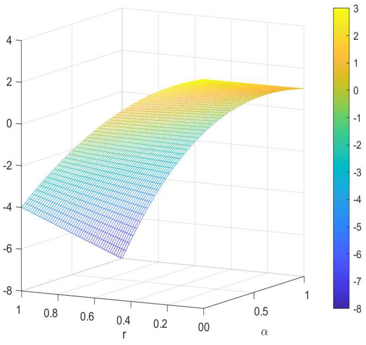
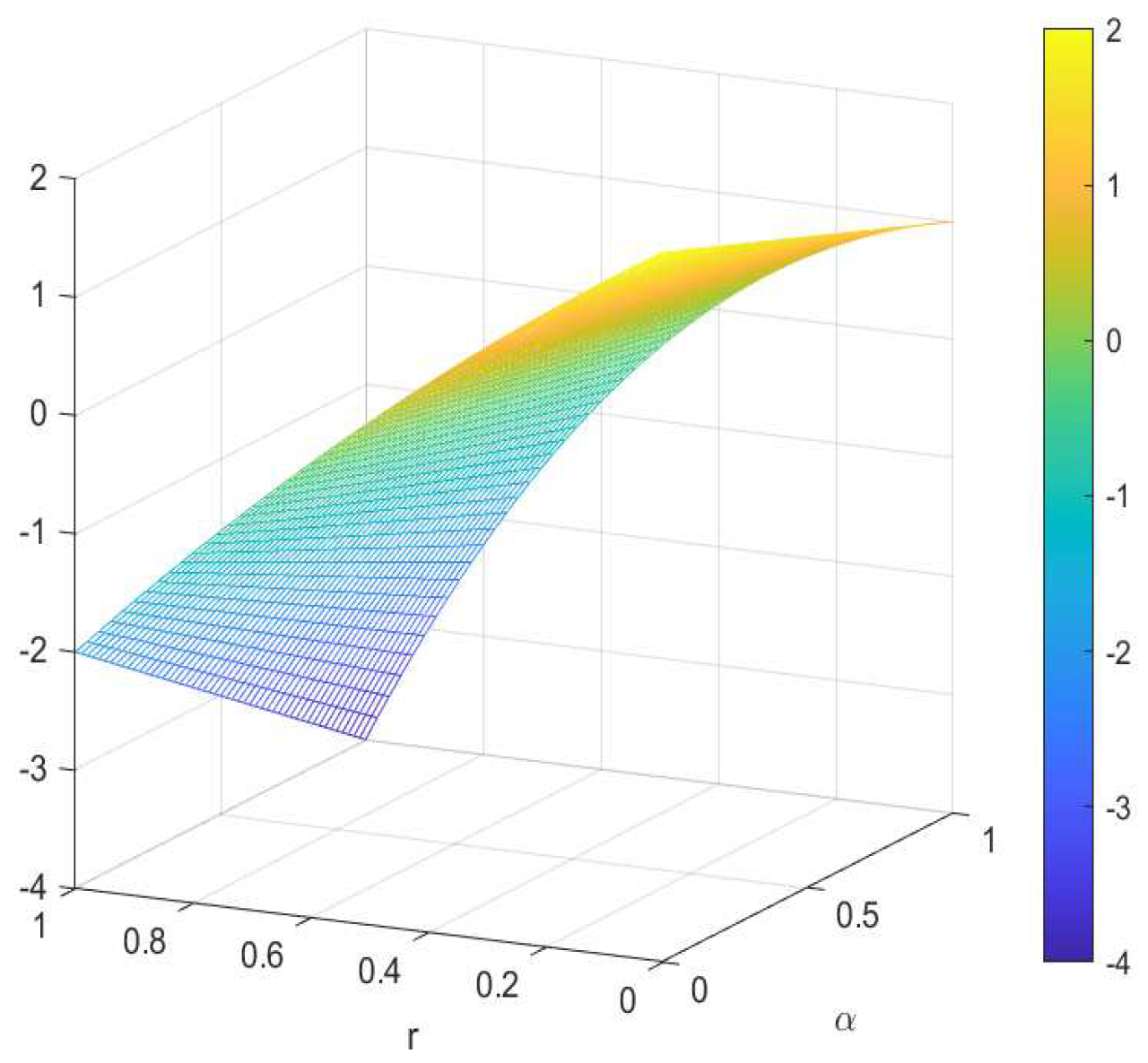
Corollary 3. 

Let $\alpha \in (0,1)$ and $\left|z\right|=r<1$. If the function $f\in HR{K}_{sc}^{\alpha }(1,\frac{1}{2})$, then the Bloch constant ${\mathcal{B}}_f$ of f is bounded and

$${\mathcal{B}}_f\le \frac{(1+\alpha )(1-r_3^2)(1+r_3){(1-r_3)}^{-\frac{1}{2}}}{1+\alpha r_3},$$

where $r_3$ is the only root of equation

$$\begin{array}{c}\hfill 2(1+\alpha r)(1-2r-3r^2)+(1-2\alpha +3\alpha r){(1+r)}^2=0\end{array}$$

in the interval $(0,1)$, and the image of function

$$\mathcal{M}(r,\alpha )=2(1+\alpha r)(1-2r-3r^2)+(1-2\alpha +3\alpha r){(1+r)}^2$$

(37)

is shown in Figure 1. In the figure, the function $\mathcal{M}(r,\alpha )$ is represented by the three-dimensional coordinate system plus color; the $x-$axis represents the variable α; the $y-$axis represents the variable r; the $z-$axis and color represents the function $\mathcal{M}(r,\alpha )$.

Corollary 4. 

Let $\alpha \in (0,1)$ and $\left|z\right|=r<1$. If the function $f\in HR{K}_{sc}^{\alpha }(1,0)$, then the Bloch constant ${\mathcal{B}}_f$ of f is bounded and

$${\mathcal{B}}_f\le \frac{(1+\alpha )(1-r_4^2)(1+r_4)e^{r_4}}{1+\alpha r_4},$$

where $r_4$ is the only root of the equation

$$\begin{array}{c}\hfill (1+\alpha r)(1-3r)-(\alpha -(1+\alpha r))(1-r^2)=0\end{array}$$

in the interval $(0,1)$, and the image of function

$$\mathcal{N}(r,\alpha )=(1+\alpha r)(1-3r)-(\alpha -(1+\alpha r))(1-r^2)$$

(38)

is shown in Figure 2. In the figure, the function $\mathcal{N}(r,\alpha )$ is represented by the three-dimensional coordinate system plus color; the $x-$axis represents the variable α; the $y-$axis represents the variable r; the $z-$axis and color represents the function $\mathcal{N}(r,\alpha )$.

Next, we obtain the norm of the pre-Schwarzian derivative for the classes ${HRK}_{sc}^{\alpha }(-\frac{1}{2},-1)$.

Theorem 3. 

Let $A=-\frac{1}{2},B=-1$ and $\left|z\right|=r<1$. If $f\in {HRK}_{sc}^{\alpha }(-\frac{1}{2},-1)$, then the norm of the pre-Schwarzian derivative of f is bounded and

$$∥T_f∥⩽\frac{3(1-r_5^2)}{(2-r_5)}+\frac{2(1-{\alpha }^2)(1-r_5^2)(r_5+\alpha )}{(1+\alpha r_5)\left[(1+r_5^2)(1+{\alpha }^2)-4\alpha r_5\right]},$$

where $r_5$ is the only root of the equation

$$\begin{array}{cc}& (3r^2-12r+3){[\alpha (1+{\alpha }^2)r^3+(1-3{\alpha }^2)r^2+\alpha ({\alpha }^2-3)r+1+{\alpha }^2]}^2\hfill \\ & +2(1-{\alpha }^2){(2-r)}^2[({\alpha }^4+4{\alpha }^2-1)r^4+4\alpha (1-{\alpha }^2)r^3\hfill \\ & -4(1+{\alpha }^4)r^2+4\alpha ({\alpha }^2-1)r+1+4{\alpha }^2-{\alpha }^4]=0\hfill \end{array}$$

in the interval $(0,1)$.

In particular, let $\alpha =\frac{1}{2}$. The norm of the pre-Schwarzian derivative of f is bounded and

$$\begin{array}{cc}\hfill ∥T_f∥& ⩽\frac{3(1-r_6^2)}{(2-r_6)}+\frac{6(2r_6+1)(1-r_6^2)}{(2+r_6)(5r_6^2-8r_6+5)},\hfill \end{array}$$

where $r_6\approx 0.4975$ is the only root of the equation

$$75r^8-240r^7-477r^6+1620r^5-1467r^4-360r^3+2553r^2-3180r+1044=0.$$

Proof. 

Suppose that $f=h+\overline{g}\in {HRK}_{sc}^{\alpha }(-\frac{1}{2},-1)$, then $h\in {RK}_{sc}(-\frac{1}{2},-1)$. Applying Lemma 4, we have

$$\left|T_h\right|=\left|\frac{h^{″}}{h^{\prime }}\right|\le \frac{\frac{3}{2}}{(1-\frac{1}{2}r)}.$$

(39)

We can obtain from Lemma 5 and the inequality (39) that

$$\left|T_f\right|=\left|\frac{h^{″}}{h^{\prime }}+\frac{2w^{\prime }\overline{w}}{1+{\left|w\right|}^2}\right|⩽\left|T_h\right|+\frac{2\left|w^{\prime }\right|\left|\overline{w}\right|}{1+{\left|w\right|}^2}.$$

and

$$\begin{array}{cc}\hfill ∥T_f∥& \le \underset{0<r<1}{sup}\left[\frac{(1-r^2)\left(\frac{3}{2}\right)}{(1-\frac{1}{2}r)}+\frac{2\left(1-{\alpha }^2\right)(1-r^2)(r+\alpha )}{(1+\alpha r)\left[\left(1+r^2\right)\left(1+{\alpha }^2\right)-4\alpha r\right]}\right].\hfill \end{array}$$

(40)

Let

$${\mathbb{F}}_{\alpha }\left(r\right)=\frac{3(1-r^2)}{(2-r)}+\frac{2\left(1-{\alpha }^2\right)(1-r^2)(r+\alpha )}{(1+\alpha r)\left[\left(1+r^2\right)\left(1+{\alpha }^2\right)-4\alpha r\right]},$$

then

$${\mathbb{F}}_{\alpha }^{\prime }\left(r\right)=\frac{3r^2-12r+3}{{(2-r)}^2}+\frac{2\left(1-{\alpha }^2\right)\mathcal{V}(\alpha ,r)}{{\left\{(1+\alpha r)\left[\left(1+r^2\right)\left(1+{\alpha }^2\right)-4\alpha r\right]\right\}}^2},$$

(41)

where

$$\mathcal{V}(\alpha ,r)=\left({\alpha }^4+4{\alpha }^2-1\right)r^4+4\alpha \left(1-{\alpha }^2\right)r^3-4\left(1+{\alpha }^4\right)r^2+4\alpha \left({\alpha }^2-1\right)r+1+4{\alpha }^2-{\alpha }^4.$$

It can be seen from (41) that ${\mathbb{F}}_{\alpha }^{\prime }\left(r\right)=0$ is true if and only if ${\mathbb{T}}_{\alpha }\left(r\right)=0$ is true, where

$$\begin{array}{cc}\hfill {\mathbb{T}}_{\alpha }\left(r\right)=& (3{\alpha }^6+6{\alpha }^4+3{\alpha }^2)r^8+(-12{\alpha }^6-18{\alpha }^5-24{\alpha }^4-12{\alpha }^3-12{\alpha }^2+6\alpha )r^7\hfill \\ & +(7{\alpha }^6+72{\alpha }^5+15{\alpha }^4+48{\alpha }^3-23{\alpha }^2-24\alpha +1)r^6\hfill \\ & +(-16{\alpha }^6-22{\alpha }^5-36{\alpha }^4+44{\alpha }^3+104{\alpha }^2+2\alpha -4)r^5\hfill \\ & +(9{\alpha }^6+16{\alpha }^5-53{\alpha }^4-224{\alpha }^3+27{\alpha }^2+16\alpha -7)r^4\hfill \\ & +(-44{\alpha }^6+18{\alpha }^5+176{\alpha }^4+12{\alpha }^3-92{\alpha }^2-6\alpha +8)r^3\hfill \\ & +(37{\alpha }^6+8{\alpha }^5-75{\alpha }^4-16{\alpha }^3+59{\alpha }^2+104\alpha -21)r^2\hfill \\ & +(-8{\alpha }^6-26{\alpha }^5+28{\alpha }^4+52{\alpha }^3-48{\alpha }^2-50\alpha -20)r\hfill \\ & +8{\alpha }^6-37{\alpha }^4+30{\alpha }^2+11.\hfill \end{array}$$

(42)

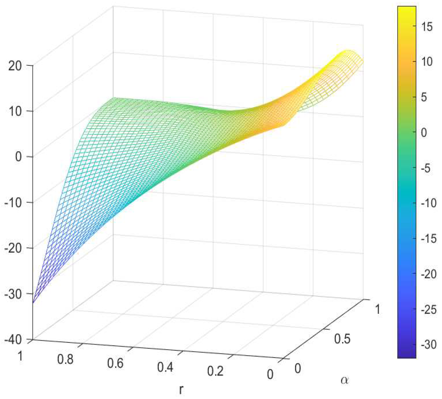
The image of ${\mathbb{T}}_{\alpha }\left(r\right)$ is shown Figure 3 because ${\mathbb{T}}_{\alpha }\left(r\right)$ is continuous in the interval $[0,1]$ and satisfies the condition

$$\begin{array}{cc}\hfill {\mathbb{T}}_{\alpha }\left(0\right)=& 8{\alpha }^6-37{\alpha }^4+30{\alpha }^2+11>0,{\mathbb{T}}_{\alpha }\left(1\right)=-16{(1+\alpha )}^2{(1-\alpha )}^3(2-\alpha )<0.\hfill \end{array}$$

Therefore, there is at least a root $r_5\in (0,1)$, such that ${\mathbb{T}}_{\alpha }\left(r_5\right)=0$.

In particular, let $\alpha =\frac{1}{2}$. From (40), we have

$$\begin{array}{cc}\hfill ∥T_f∥& ⩽\underset{0<r<1}{sup}\frac{3(1-r^2)}{(2-r)}+\frac{6(2r+1)(1-r^2)}{(2+r)(5r^2-8r+5)}.\hfill \end{array}$$

Let

$$\mathbb{F}\left(r\right)=\frac{3(1-r^2)}{(2-r)}+\frac{6(2r+1)(1-r^2)}{(2+r)(5r^2-8r+5)},$$

we obtain

$${\mathbb{F}}^{\prime }\left(r\right)=\frac{\mathbb{T}\left(r\right)}{{(2-r)}^2{\left((2+r)(5r^2-8r+5)\right)}^2}.$$

(43)

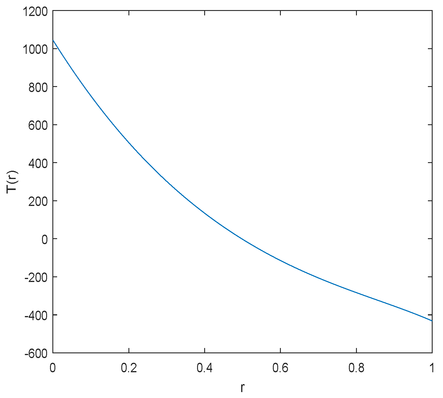
It can be seen from (43) that ${\mathbb{F}}^{\prime }\left(r\right)=0$ is true if and only if $\mathbb{T}\left(r\right)=0$ is true, where

$$\begin{array}{c}\hfill \mathbb{T}\left(r\right)=75r^8-240r^7-477r^6+1620r^5-1467r^4-360r^3+2553r^2-3180r+1044.\end{array}$$

(44)

The image of $\mathbb{T}\left(r\right)$ is shown Figure 4 because $\mathbb{T}\left(r\right)$ is continuous in the interval $[0,1]$ and satisfies the condition

$$\begin{array}{cc}\hfill \mathbb{T}\left(0\right)=& 1044>0,\mathbb{T}\left(1\right)=-432<0.\hfill \end{array}$$

As a result, there is only one $r_6\in (0,1)$, which makes $\mathbb{T}\left(r_6\right)=0$. According to the geometric properties of the function $\mathbb{F}\left(r\right)$, $\mathbb{F}\left(r\right)$ takes the maximum value at $r_6$. □

4. Conclusions

In this paper, by means of subordination, we introduce some classes of univalent harmonic functions with respect to the symmetric conjugate points. the analytic parts of which are reciprocal starlike (or convex) functions. Further, by combining with the graph of the function, we discuss the bound of Bloch constant and the norm of pre-Schwarzian derivative for the classes, which can enrich the research field of univalent harmonic mapping.