The Generalized Classes of Linear Symmetric Subdivision Schemes Free from Gibbs Oscillations and Artifacts in the Fitting of Data

Abstract

This paper presents the advanced classes of linear symmetric subdivision schemes for the fitting of data and the creation of geometric shapes. These schemes are derived from the B-spline and Lagrange’s blending functions. The important characteristics of the derived schemes, including continuity, support, and the impact of parameters on the magnitude of the artifact and Gibbs oscillations are discussed. Schemes additionally generalize various subdivision schemes. Linear symmetric subdivision schemes can produce Gibbs oscillations when the initial data is taken from discontinuous functions. Additionally, these schemes may generate unwanted artifacts in the limit curve that do not exist in the original polygon. One solution is to use non-linear schemes, but this approach increases the computational complexity of the scheme. An alternative approach is proposed that involves modifying the linear symmetric schemes by introducing parameters into the linear rules. The suitable values of these parameters reduce or eliminate Gibbs oscillations and artifacts while still using linear symmetric schemes. Our approach provides a balance between reducing or eliminating Gibbs oscillations and artifacts while maintaining computational efficiency.

In the second half, the piecewise parametric polynomial curves by using the blending polynomials used in the symmetric schemes are also presented. The majority of the properties of uniform quadratic and cubic B-splines with $G^2$ geometric continuities are inherited by these polynomial curves. These curves can also be used for local interpolation of the control points with $G^2$ continuity. Furthermore, by adjusting the value of the shape parameter, uniform cubic and quadratic B-spline curves can also be produced. These polynomial curves also satisfy the shape preserving properties of initial data.

1. Introduction

One common technique for designing curves and surfaces is the subdivision scheme. They give an exact and effective way to describe curves and surfaces that are smooth and nice as the limit of a sequence of consecutive refinements. It is an algorithmic technique through which, after successive iterations, a smooth curve or surface is obtained as the data is applied to a dense union of points. Subdivision schemes can be categorized into two types: symmetric and nonsymmetric schemes. The rules used in symmetric schemes are both shift and flip invariant. Symmetric schemes are frequently used in the literature as a standard technique for smoothing out coarse polygons or shapes. Their magnificence lies in their exquisite mathematical formulation and simple implementation.

Dyn et al. [1] proposed refinement rules by evaluating cubic polynomials based on local cubic interpolation. Ko et al. [2] proposed a more efficient ternary approximating 4-point subdivision scheme deduced from interpolating the cubic polynomial. In addition, they generalized ternary $(2n+2)$-point subdivision schemes. Hussain et al. [3] established a generalised family of 5-point schemes with different arity and shape determining parameter. Rehan and Siddiqi [4] presented a class of ternary subdivision schemes having a complexity of 3 that generate $C^1$ curves. They also suggested that the limiting curves of $C^3$ can be generated from a 4-point approximating ternary subdivision scheme. The approximating subdivision schemes having arbitrary complexity with a single parameter were presented by Mustafa et al. [5] and [6]. They showed that their schemes are better in contrast with the various existing subdivision schemes. Dual de Rham-type subdivision schemes were developed by Conti and Romani [7]. These are smoother, with a modest increase in the support width. Zhang et al. [8] presented Hermite subdivision schemes of any arity. They estimated their smoothness as well. Wang and Ma [9] presented an extended, tuned subdivision strategy for quadrilateral meshes.

Nawaz et al. [10] discussed various properties of a 7-point approximating quaternary subdivision scheme. Zouaoui et al. [11] examined the design and analysis of certain novel n-point families for ternary subdivision schemes. Iqbal et al. [12] discussed the influence of a geometric characteristic on curve sketching using the tension parameter. Amat et al. [13] suggested that the 4-point ternary non-linear non-interpolatory subdivision scheme may eliminate the Gibbs phenomenon. Later, Zhou et al. [14] developed a sufficient condition to test the hypothesis that p-ary subdivision schemes exhibit the Gibbs phenomenon in the limit function at the discontinuous point. Yan et al. [15] assembled a collection of surface and curve subdivision schemes.

Artifacts are caused by differences between mathematical modeling and the practical imaging process. All users should be aware of their existence and be prepared to deal with them in the event they occur. This phenomenon [16] can disrupt the diagnostic process for CBCT data sets. Digital artifacts are irregularities that digital signal processing introduces into digital signals. Artifacts are inaccurate representations of tissue structures created in EEG, ultrasound, X-ray, CT scan, and magnetic resonance imaging in medical imaging (MRI). The shadow effect [17] may result in measurement noise or artifact in the raw data because of the way the laser scanner is made. The PPG signal from pulse oximeters frequently becomes saturated and clipped due to artifacts [18]. Cone-beam computed tomography (CBCT) scans suffer from poor picture quality due to artifacts, which may make it more difficult to diagnose certain illnesses [19]. As a result, determining the size of the artifact is required.

In CAGD, modifying the shape of curves and surfaces by choosing a suitable value for shape parameters is an extremely popular topic for discussion. To increase the flexibility of the curve, it is extremely necessary to adjust the shape parameter’s value. We can adjust the shape of the curve for practical applications more conveniently by assigning different values to a parameter. The prior research utilizing shape parameters to deal with the curve shape design problem was proposed by Barsky [20]. Costantini [21] studied how to build variable-degree polynomials, which have the same structure and features as cubics but have more flexibility over their shape. Farouki et al. [22] investigated the preservation property of PH splines. The parametric curve maintains the form of planar data by modifying tension parameters. An addition of cubic uniform B-spline curves with most characteristics identical to the corresponding cubic uniform B-spline curves without parameters was proposed by Xu and Wang [23]. Han and Yang [24] depicted a piecewise curve with locally modifiable shape parameters. Cao and Wang [25] presented a correlation between the B-spline basis functions and the uniform B-spline basis functions having a parameter. As an extension of the characteristics of shape-preserving function curves, ref. [26] redefined parametric curves and investigated the impact of polynomial functions on flying trajectories.

Linear symmetric subdivision schemes can produce Gibbs oscillations [14] when the initial data is derived from discontinuous functions. Additionally, these schemes may generate unwanted artifacts in the geometric shapes, which do not exist in the original polygon or sketch but appear in the limit curve produced by the schemes. To address these issues, one solution is to use non-linear symmetric schemes, but this approach increases the computational complexity of the method. To address this challenge, we propose an alternative approach that involves modifying the linear symmetric schemes by introducing shape parameters into the linear rules. By choosing the values of these parameters, we can overcome these issues while still using linear symmetric schemes. Our approach provides a balance between reducing artifacts and maintaining computational efficiency.

This work belongs to the field of computational geometry and finds applications in the graphical modelling of curves and surfaces. Additionally, it contributes to the development of shape-preserving models used in engineering and industry. It also offers applications in digital signal processing.

This paper is arranged as follows: Basic definitions and essential prerequisite formulas are provided in Section 2. Section 3, Section 4 and Section 5 develop a general parametric family of n-ary linear symmetric subdivision schemes by combining B-spline and Lagrange’s basis functions. Some properties of the members of proposed classes are discussed in Section 6. In Section 7, some features of the piecewise polynomial curve are discussed. In Section 8, some applications, examples, and comparisons with existing schemes are discussed to show the efficiency of the proposed schemes. The conclusion is given in Section 9.

2. Preliminaries and Notations

We review some fundamentally relevant definitions and known concepts about subdivision schemes in this section because they form the foundation of the rest of this paper.

If $p^k$ = ${\left\{p_{\varrho }^k\right\}}_{\varrho \in \mathbb{Z}}$ and $p^{k+1}$ = ${\left\{p_{\varrho }^{k+1}\right\}}_{\varrho \in \mathbb{Z}}$ are two k-th and $(k+1)$-th level polygons, followed by the n-ary linear symmetric subdivision scheme, which generates $p^{k+1}$ from $p^k$ presented by [27] is:

$$p_{n\varrho +l}^{k+1}=\sum _{\gamma \in \mathbb{Z}}{\varsigma }_{n\gamma +l}{p}_{\varrho -\gamma }^k,\varrho \in \mathbb{Z},0\le l\le n-1,$$

(1)

where n indicates the arity of the subdivision scheme and the sequence $\varsigma =\{{\varsigma }_{\varrho }:\varrho \in \mathbb{Z}\}$ of a finite number of coefficients determines the mask of the subdivision scheme. The subdivision scheme (1) satisfies the following necessary condition

$$\sum _{\gamma \in \mathbb{Z}}{\varsigma }_{n\gamma +l}=1,0\le l\le n-1.$$

For the mask $\varsigma$, the z-transform is given below to examine the subdivision scheme’s features.

$$L\left(z\right)=\sum _{\varrho \in \mathbb{Z}}{\varsigma }_{\varrho }{z}^{\varrho },z\in \mathbb{C}\setminus \left\{0\right\}.$$

(2)

Equation (2) is usually known as the Laurent polynomial or symbol of the scheme.

A B-spline curve [28] is defined as a linear combination of control points $p_m$ and B-spline blending function ${\Re }_{m,k}\left(t\right)$.

$$P\left(t\right)=\sum _{m=0}^n{p}_m{\Re }_{m,k}\left(t\right),n⩾k-1,$$

where $p_m,m=0,1,2,\dots ,n$, are control points. The B-spline blending functions are defined recursively for $k>1$ as

$$\begin{array}{cc}\hfill {\Re }_{m,k}\left(t\right)=\left(\frac{t-t_m}{t_{m+k-1}-t_{\varrho }}\right)& {\Re }_m{,}_{k-1}\left(t\right)+\left(\frac{t_{m+k}-t}{t_{m+k}-t_{m+1}}\right){\Re }_{m+1}{,}_{k-1}\left(t\right),\hfill \end{array}$$

(3)

and for $k=1$, we can write the blending functions as

$${\Re }_{m,1}\left(t\right)=\left\{\begin{array}{c}1\mathrm{if}t\in [t_m,t_{m+1}),\hfill \\ 0\mathrm{otherwise},\hfill \end{array}\right.$$

(4)

where k is the curve’s order and $\{t_0,t_1,\dots ,t_{n+k}\}$ is the non-decreasing sequence of uniform knots.

The Lagrange polynomials $\overline{Q}\left(t\right)$ for Lagrange basis ${\left\{{\mathbb{L}}_j\left(t\right)\right\}}_{j=-N}^{N+\nu }$ corresponding to the nodes ${\left\{j\right\}}_{-N}^{N+\nu }$ is defined by

$$\overline{Q}\left(t\right)=\sum _{j=-N}^{N+\nu }{\mathbb{L}}_j\left(t\right)p_j,{\mathbb{L}}_j\left(t\right)=\prod _{k=-N,k\ne j}^{N+\nu }\left(\frac{t-k}{j-k}\right),N=1,2,\dots$$

When $\nu =0$, an even-degree polynomial is obtained, and when $\nu =1$, an odd-degree polynomial is obtained. From the derivation of the polynomial interpolation property, the mask can be obtained. The initial data $(\varrho +j,p_{\varrho +j}^0)$, $j=-N,\dots ,N+\nu$, is interpolated by a polynomial, and then at $\varrho +\frac{2j+1}{2s}$, for $s=2,3,4\dots$ and $j=0,1,2\dots$, the data is evaluated. Since up to a fixed degree the space of polynomials are shift invariant and the scheme is stationary and uniform, we only deal with the case for both k and $\varrho =0$ (for details, see [1]).

3. Construction of Binary Odd-Point Symmetric Scheme

This section is devoted to deriving a general formula for obtaining the class of 3-point binary approximating stationary subdivision schemes having a parameter. At the $(k+1)$-th level, we consider subdivision schemes that generate the refined data $p^{k+1}={\left\{p_{\varrho }^{k+1}\right\}}_{\varrho \in \mathbb{Z}}$ for any $k\in \mathbb{N}$.

$$\left\{\begin{array}{ccc}{p}_{2\varrho }^{k+1}& =& \sum _{\tau \in J_{\varrho }^k}{d}^k{p}_{\varrho -\tau }^k,\\ p_{2\varrho +1}^{k+1}& =& \sum _{\tau \in J_{\varrho }^k}{e}^k{p}_{\varrho -\tau }^k,\end{array}\right.$$

where $J_{\varrho }^k\subset \mathbb{Z}$ is a finite set and weights $d^k,e^k\in \mathbb{R}$, for $\varrho \in \{0,1,2,\dots ,2^k-1\}$, $\tau \in J_{\varrho }^k$, and $k\in \mathbb{N}$. If all sets $J_{\varrho }^k$ have the same cardinality r then the subdivision scheme is known as the r-point scheme.

For a 3-point scheme with $J_{\varrho }^k=\{-1,0,1\}$, weights $d^k$=$({\Omega }^k,{\gamma }^k,{\delta }^k)$ and $e^k$=$({\delta }^k,{\gamma }^k,{\Omega }^k)$, the new data values $p_{2\varrho }^{k+1}$ and $p_{2\varrho +1}^{k+1}$ are the linear combination of data values $p_{\varrho -1}^k,p_{\varrho }^k,p_{\varrho +1}^k$

$$\left\{\begin{array}{ccc}{p}_{2\varrho }^{k+1}& =& {\Omega }^k{p}_{\varrho -1}^k+{\gamma }^k{p}_{\varrho }^k+{\delta }^k{p}_{\varrho +1}^k,\\ p_{2\varrho +1}^{k+1}& =& {\delta }^k{p}_{\varrho -1}^k+{\gamma }^k{p}_{\varrho }^k+{\Omega }^k{p}_{\varrho +1}^k.\end{array}\right.$$

(5)

Here we see that the weights $d^k$=$({\Omega }^k,{\gamma }^k,{\delta }^k)$ and $e^k$=$({\delta }^k,{\gamma }^k,{\Omega }^k)$, are both shift and flip invariant, so the scheme is called symmetric. Alternatively, the rules $p_{2\varrho }^{k+1}$ and $p_{2\varrho +1}^{k+1}$ are both shift and flip invariant, so the scheme is symmetric. Here we find the condition for choosing a suitable weight such that the 3-point subdivision scheme generates a $C^2$ limit function. Because the weights in the rules are independent of the subdivision level k, we use $k=1$. Let us consider a piecewise quadratic B-spline that can be represented as

$$\begin{array}{c}\hfill P\left(t\right)=\sum _{m=0}^2{\Re }_{m,3}\left(t\right)p_m,t\in [\varrho -1,\varrho ]\subset [0,n-1],\varrho =1,2,\dots ,n,\end{array}$$

(6)

where, ${\Re }_{m,3}\left(t\right)$, $m=0,1,2$ are the basis functions. The basis functions of a quadratic B-spline at the uniform knots $\{1,2,3,\dots \}$ are

$$\begin{array}{cc}\hfill {\Re }_{0,3}\left(t\right)=& \frac{1}{2}{(1-t)}^2,{\Re }_{1,3}\left(t\right)=\frac{1}{2}(1+2t-2t^2),{\Re }_{2,3}\left(t\right)=\frac{1}{2}{\left(t\right)}^2.\hfill \end{array}$$

Replacing $p_0,p_1,p_2$ with $p_{\varrho -1}^k,p_{\varrho }^k,p_{\varrho +1}^k$, we can write (6) in matrix notation as

$$P\left(t\right)=\left(\begin{array}{c}1t{t}^2\end{array}\right)M_1\left(\begin{array}{c}{p}_{\varrho -1}^k\\ p_{\varrho }^k\\ p_{\varrho +1}^k\end{array}\right),$$

(7)

where

$$M_1=\frac{1}{2}{\left(\begin{array}{ccc}1& -2& 1\\ 1& 2& -2\\ 0& 0& 1\end{array}\right)}^T.$$

We can write the Lagrange basis function of a quadratic polynomial in matrix notation at the node points $\{-1,0,1\}$ and sample the data $(j,p_j)$ at $j=\varrho -1,\varrho ,\varrho +1$.

$$\overline{Q}\left(t\right)=\left(\begin{array}{c}1t{t}^2\end{array}\right)N_1\left(\begin{array}{c}{p}_{\varrho -1}^k\\ p_{\varrho }^k\\ p_{\varrho +1}^k\end{array}\right),$$

(8)

where

$$N_1=\frac{1}{2}\left(\begin{array}{ccc}0& 2& 0\\ 1& 0& -1\\ 1& -2& 1\end{array}\right).$$

We get the displacement vector $D\left(t\right)$ by taking the difference between (8) and (7).

$$D\left(t\right)=\left(\frac{-1}{2}+\frac{3t}{2}\right)p_{\varrho -1}^k+\left(\frac{1}{2}-t\right)p_{\varrho }^k-\left(\frac{1}{2}t\right)p_{\varrho +1}^k.$$

Now to obtain the newly inserted vertices, the following equation is established:

$$p_{n\varrho +r}^{k+1}=P\left(t\right)+\alpha D\left(t\right).$$

(9)

This implies

$$\begin{array}{ccc}\hfill p_{n\varrho +r}^{k+1}\left(t\right)& =& \frac{1}{2}\left[(1-\alpha )+(3\alpha -2)t+t^2\right]p_{\varrho -1}^k+\frac{1}{2}\left[(1+\alpha )+2(1-\alpha )t-2t^2\right]p_{\varrho }^k\hfill \\ & & +\frac{1}{2}\left[-\left(\alpha \right)t+t^2\right]p_{\varrho +1}^k.\hfill \end{array}$$

The above polynomial can be expressed as

$$p_{n\varrho +r}^{k+1}\left(t\right)=\left(\begin{array}{c}1t{t}^2\end{array}\right)L_1\left(\begin{array}{c}{p}_{\varrho -1}^k\\ p_{\varrho }^k\\ p_{\varrho +1}^k\end{array}\right),$$

(10)

where

$$L_1=\frac{1}{2}\left(\begin{array}{ccc}1-\alpha & \alpha +1& 0\\ 3\alpha -2& 2(1-\alpha )& -\alpha \\ 1& -2& 1\end{array}\right).$$

Now evaluate the polynomial (10) at $n=2$, $r=0,1$ and $t=\frac{1}{4}$ to obtain the points at $(k+1)$-th subdivision level of 3-point binary scheme.

$$\left\{\begin{array}{c}\begin{array}{cc}\hfill p_{2\varrho }^{k+1}=& \left(\frac{9}{32}-\frac{1}{8}\alpha \right)p_{\varrho -1}^k+\left(\frac{11}{16}+\frac{1}{4}\alpha \right)p_{\varrho }^k+\left(\frac{1}{32}-\frac{1}{8}\alpha \right)p_{\varrho +1}^k,\hfill \\ \hfill p_{2\varrho +1}^{k+1}=& \left(\frac{1}{32}-\frac{1}{8}\alpha \right)p_{\varrho -1}^k+\left(\frac{11}{16}+\frac{1}{4}\alpha \right)p_{\varrho }^k+\left(\frac{9}{32}-\frac{1}{8}\alpha \right)p_{\varrho +1}^k.\hfill \end{array}\end{array}\right.$$

(11)

It is also presented in Algorithm 1.

Algorithm 1: The subdivision levels of the 3-point binary subdivision scheme with shape parameter $\alpha$

Input: Coarse data ${\left\{p_{\varrho }\right\}}_{\varrho \in \mathbb{Z}}$ Output: Refine data is obtained.  $p_{2\varrho }^0$←$p_{\varrho }$  $p_{2\varrho +1}^0$←$p_{\varrho }$  $\Omega :=\left(\frac{9}{32}-\frac{1}{8}\alpha \right)$: $\gamma :=\left(\frac{11}{16}+\frac{1}{4}\alpha \right)$: $\delta :=\left(\frac{1}{32}-\frac{1}{8}\alpha \right)$:  for ℏ∈$\mathbb{N}$ do     for $\varrho$∈$\mathbb{Z}$ do        $p_{2\varrho }^{\hslash ,0}$←$\Omega p_{\varrho -1}^{\hslash -1}+\gamma p_{\varrho }^{\hslash -1}+\delta p_{\varrho +1}^{\hslash -1}$        $p_{2\varrho +1}^{\hslash ,0}$←$\delta p_{\varrho -1}^{\hslash -1}+\gamma p_{\varrho }^{\hslash -1}+\Omega p_{\varrho +1}^{\hslash -1}$     end for $\left(\varrho \right)$     for $k=1,2,\dots ,m-1$ do        for $\varrho$∈$\mathbb{Z}$ do           $p_{2\varrho }^{\hslash ,k}$←$\Omega p_{\varrho -1}^{\hslash ,k-1}+\gamma p_{\varrho }^{\hslash ,k-1}+\delta p_{\varrho +1}^{\hslash ,k-1}$           $p_{2\varrho +1}^{\hslash ,k}$←$\delta p_{\varrho -1}^{\hslash ,k-1}+\gamma p_{\varrho }^{\hslash ,k-1}+\Omega p_{\varrho +1}^{\hslash ,k-1}$        end for $\left(\varrho \right)$     end for $\left(k\right)$     for $\varrho$∈$\mathbb{Z}$ do        $p_{\varrho }^{\hslash }$←$p_{\varrho }^{\hslash ,m-1}$     end for $\left(\varrho \right)$  end for $(\hslash )$

Similarly, we can obtain a 5-point binary symmetric subdivision scheme by considering the quartic Lagrange and B-spline polynomials.

$$\left\{\begin{array}{c}\begin{array}{cc}\hfill p_{2\varrho }^{k+1}=& \left(\frac{27}{2048}-\frac{9\alpha }{256}\right)p_{\varrho -2}^k+\left(\frac{499}{1536}-\frac{23\alpha }{192}\right)p_{\varrho -1}^k+\left(\frac{1723}{3072}+\frac{139\alpha }{384}\right)p_{\varrho }^k\hfill \\ & +\left(\frac{155}{1536}-\frac{43\alpha }{192}\right)p_{\varrho +1}^k+\left(\frac{1}{6144}+\frac{13\alpha }{768}\right)p_{\varrho +2}^k,\hfill \\ \hfill p_{2\varrho +1}^{k+1}=& \left(\frac{1}{6144}+\frac{13\alpha }{768}\right)p_{\varrho -2}+\left(\frac{155}{1536}-\frac{43\alpha }{192}\right)p_{\varrho -1}+\left(\frac{1723}{3072}+\frac{139\alpha }{384}\right)p_{\varrho }\hfill \\ & +\left(\frac{499}{1536}-\frac{23\alpha }{192}\right)p_{\varrho +1}+\left(\frac{27}{2048}-\frac{9\alpha }{256}\right)p_{\varrho +2}.\hfill \end{array}\end{array}\right.$$

(12)

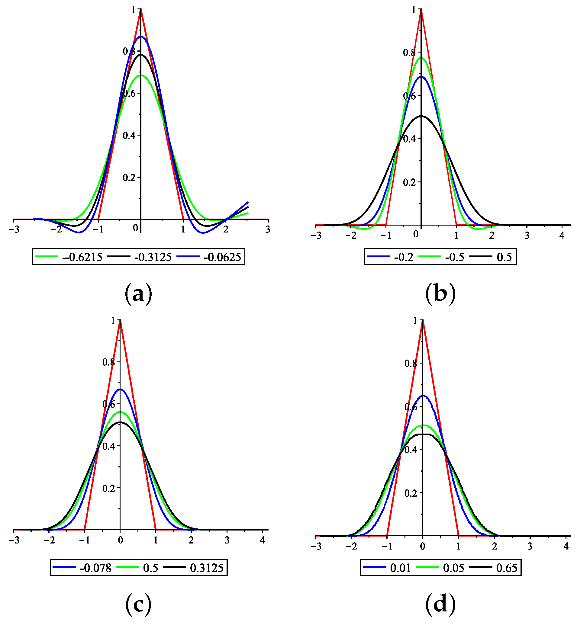
In this paper, the order of the continuity of the schemes are computed by using the Algorithm 1 of [29]. The effect of the parameter $\alpha$ on the order of continuity of the scheme (11) is shown in

Table 1. For certain parameter ranges, the order of continuity of the proposed 3-point binary (11) and 5-point binary (12) schemes.

Scheme	Parameter	Continuity	Scheme	Parameter	Continuity
3-point binary	$\alpha \in (-\frac{11}{4},\frac{5}{4})$	$C^0$	5-point binary	$\alpha \in (-\frac{147}{88},\frac{109}{88})$	$C^0$
$\dots$	$\alpha \in (-\frac{11}{4},\frac{5}{4})$	$C^1$	$\dots$	$\alpha \in (-\frac{147}{88},\frac{257}{440})$	$C^1$
$\dots$	$\alpha \in (-\frac{3}{4},\frac{1}{4})$	$C^2$	$\dots$	$\alpha \in (-\frac{83}{88},\frac{45}{88})$	$C^2$
$\dots$	$\alpha =-\frac{1}{4}$	$C^4$	$\dots$	$\alpha =(-\frac{499}{632},\frac{45}{88})$	$C^3$
			$\dots$	$\alpha =(-\frac{77}{184},\frac{19}{184})$	$C^4$
				$\alpha =-\frac{5}{184}$	$C^6$

.

Remark 1.

Considering the value of $\alpha =\frac{-1}{4}$, from continuity interval, the proposed scheme (11) is converted to a $C^4$-continuous 3-point B-spline scheme and for $\alpha =\frac{-1}{4}$, we get uniform B-spline of degree 4.

4. Construction of the 4-Point $\mathbf{n}$-ary Symmetric Subdivision Schemes

In this section, we first construct a general formula to construct the 4-point n-ary subdivision scheme by blending cubic Lagrange’s and B-spline fundamental polynomials. A piecewise cubic B-spline can be represented as

$$\begin{array}{c}\hfill P\left(t\right)=\sum _{m=0}^3{\Re }_{m,4}\left(t\right)p_m,t\in [\varrho -1,\varrho ]\subset [0,n-1],\varrho =1,2,\dots ,n,\end{array}$$

where ${\Re }_{m,4}\left(t\right)$, $m=0,1,2,3$, are the basis functions. This can be expressed as

$$P\left(t\right)=\left(\begin{array}{c}1t{t}^2{t}^3\end{array}\right)M_2\left(\begin{array}{c}{p}_{\varrho -1}^k\\ p_{\varrho }^k\\ p_{\varrho +1}^k\\ p_{\varrho +2}^k\end{array}\right),$$

(13)

where $k=0,1,2,\dots ,n-3$, $t\in [0,1]$, and

$$\begin{array}{c}\hfill M_2=\frac{1}{6}{\left(\begin{array}{cccc}1& -3& 3& -1\\ 4& 0& -6& 3\\ 1& 3& 3& -3\\ 0& 0& 0& 1\end{array}\right)}^T.\end{array}$$

We can write Lagrange basis function of a cubic polynomial in matrix notation at the node points $\{-1,0,1,2\}$ and sample the data $(j,p_j)$ at $j=\varrho -1,\varrho ,\varrho +1,\varrho +2$.

$$\overline{Q}\left(t\right)=\left(\begin{array}{c}1t{t}^2{t}^3\end{array}\right)N_2\left(\begin{array}{c}{p}_{\varrho -1}^k\\ p_{\varrho }^k\\ p_{\varrho +1}^k\\ p_{\varrho +2}^k\end{array}\right),$$

(14)

where

$$\begin{array}{c}\hfill N_2=\frac{1}{6}\left(\begin{array}{cccc}0& 6& 0& 0\\ -2& -3& 6& -1\\ 3& -6& 3& 0\\ -1& 3& -3& 1\end{array}\right).\end{array}$$

Taking difference of (14) and (13), we get the following displacement vector

$$DD\left(t\right)=\left(\begin{array}{c}\frac{t-1}{6}\frac{-3t+2}{6}\frac{3t-1}{6}\frac{-t}{6}\end{array}\right)\left(\begin{array}{c}{p}_{\varrho -1}^k\\ p_{\varrho }^k\\ p_{\varrho +1}^k\\ p_{\varrho +2}^k\end{array}\right).$$

(15)

Let us consider

$$\begin{array}{ccc}\hfill p_{n\varrho +r}^{k+1}& =& P\left(t\right)+\alpha DD\left(t\right).\hfill \end{array}$$

(16)

Using (15) and (13) in (16), we get

$$\begin{array}{ccc}\hfill p_{n\varrho +r}^{k+1}\left(t\right)& =& \frac{1}{6}\left[(1-\alpha )+(\alpha -3)t+3t^2-t^3\right]p_{\varrho -1}^k+\frac{1}{6}\left[(4+2\alpha )-3\alpha t-6t^2+3t^3\right]p_{\varrho }^k\hfill \\ & & +\frac{1}{6}\left[(1-\alpha )+3(\alpha +1)t+3t^2-3t^3\right]p_{\varrho +1}^k+\frac{1}{6}(-\alpha t+t^3)p_{\varrho +2}^k.\hfill \end{array}$$

The matrix equation for the above polynomial is

$$p_{n\varrho +r}^{k+1}\left(t\right)=\left(\begin{array}{c}1t{t}^2{t}^3\end{array}\right)L_2\left(\begin{array}{c}{p}_{\varrho -1}^k\\ p_{\varrho }^k\\ p_{\varrho +1}^k\\ p_{\varrho +2}^k\end{array}\right),$$

(17)

where

$$\begin{array}{c}\hfill L_2=\frac{1}{6}\left(\begin{array}{cccc}1-\alpha & 4+2\alpha & 1-\alpha & 0\\ -3+\alpha & -3\alpha & 3\alpha +3& -\alpha \\ 3& -6& 3& 0\\ -1& 3& -3& 1\end{array}\right).\end{array}$$

4.1. The 4-Point Binary Symmetric Subdivision Scheme

We derive the 4-point binary subdivision scheme in this subsection by simply substituting $n=2$, $r=0,1$ and $t=\frac{1}{4},\frac{3}{4}$ in (17). We obtain the even and odd subdivision rules of the 4-point binary symmetric subdivision scheme as the refined data.

$$\left\{\begin{array}{c}\begin{array}{cc}\hfill p_{2\varrho }^{k+1}=& \left(\frac{9}{128}-\frac{\alpha }{8}\right)p_{\varrho -1}^k+\left(\frac{5}{24}\alpha +\frac{235}{384}\right)p_{\varrho }^k+\left(-\frac{\alpha }{24}+\frac{121}{384}\right)p_{\varrho +1}^k+\left(\frac{-\alpha }{24}+\frac{1}{384}\right)p_{\varrho +2}^k,\hfill \\ \hfill p_{2\varrho +1}^{k+1}=& \left(\frac{-\alpha }{24}+\frac{1}{384}\right)p_{\varrho -1}^k+\left(-\frac{\alpha }{24}+\frac{121}{384}\right)p_{\varrho }^k+\left(\frac{5}{24}\alpha +\frac{235}{384}\right)p_{\varrho +1}^k+\left(+\frac{9}{128}-\frac{\alpha }{8}\right)p_{\varrho +2}^k.\hfill \end{array}\end{array}\right.$$

(18)

The continuity of the above scheme at different parametric ranges of $\alpha$ is given in

Table 2. For certain parameter ranges, the order of continuity of the 4-point binary, ternary, quaternary and quinary approximating schemes.

Scheme	Parameter	Continuity	Scheme	Parameter	Continuity
Binary	$\alpha \in (-\frac{59}{16},\frac{37}{16})$	$C^0$	Quaternary	$\alpha \in (-\frac{721}{64},\frac{791}{64})$	$C^0$
$\dots$	$\alpha \in (-\frac{59}{16},\frac{37}{16})$	$C^1$	…	$\alpha \in (-\frac{27}{8},\frac{21}{8})$	$C^1$
$\dots$	$\alpha \in (-\frac{35}{16},\frac{13}{16})$	$C^2$	…	$\alpha \in (-\frac{85}{64},\frac{107}{64})$	$C^2$
$\dots$	$\alpha \in (-\frac{35}{16},\frac{13}{16})$	$C^3$	…	$\alpha \in (-\frac{13}{64},\frac{35}{64})$	$C^3$
$\dots$	$\alpha \in (-\frac{11}{16},\frac{1}{16})$	$C^4$	…	$\alpha =\frac{11}{64}$	$C^4$
$\dots$	$\alpha =-\frac{5}{16}$	$C^6$	Quinary	$\alpha \in (-\frac{1847}{50},\frac{1903}{50})$	$C^0$
Ternary	$\alpha \in (-\frac{139}{36},\frac{185}{36})$	$C^0$	…	$\alpha \in (-\frac{253}{100},\frac{347}{100})$	$C^1$
$\dots$	$\alpha \in (-\frac{79}{36},\frac{131}{36})$	$C^1$	…	$\alpha \in (-\frac{97}{100},\frac{143}{100})$	$C^2$
$\dots$	$\alpha \in (-\frac{49}{36},\frac{95}{36})$	$C^2$	…	$\alpha \in (-\frac{1}{4},\frac{71}{100})$	$C^3$
$\dots$	$\alpha \in (-\frac{61}{36},\frac{83}{36})$	$C^3$
$\dots$	$\alpha =\frac{7}{36}$	$C^4$

.

Remark 2.

• For $\alpha =\frac{-5}{16}$ the scheme (18) is converted to a 4-point B-spline which produces $C^6$-continuous curves.
• For $\alpha =\frac{1}{16}$ the scheme (18) is converted to a 3-point B-spline which produces $C^4$-continuous curve.

4.2. The 4-Point Ternary Symmetric Subdivision Scheme

Here, our main concern is to exhibit a subdivision scheme with high smoothness and minimum support. To obtain our goal, we follow the same approach that is used at the beginning of Section 4. We obtain the following rules of a 4-point symmetric ternary scheme by substituting $n=3$, $r=0,1,2$ and $t=\frac{1}{6},\frac{3}{6},\frac{5}{6}$ in (17).

$$\left\{\begin{array}{c}\begin{array}{cc}\hfill p_{3\varrho }^{k+1}=& \left(\frac{125}{1296}+\frac{5\alpha }{36}\right)p_{\varrho -1}^k+\left(\frac{277}{432}-\frac{1\alpha }{4}\right)p_{\varrho }^k+\left(\frac{113}{432}+\frac{\alpha }{12}\right)p_{\varrho +1}^k+\left(\frac{1}{1296}+\frac{\alpha }{36}\right)p_{\varrho +2}^k,\hfill \\ \hfill p_{3\varrho +1}^{k+1}=& \left(\frac{1}{48}+\frac{\alpha }{12}\right)p_{\varrho -1}^k+\left(\frac{23}{48}-\frac{1\alpha }{12}\right)p_{\varrho }^k+\left(\frac{23}{48}-\frac{\alpha }{12}\right)p_{\varrho +1}^k+\left(\frac{1}{48}+\frac{\alpha }{12}\right)p_{\varrho +2}^k,\hfill \\ \hfill p_{3\varrho +2}^{k+1}=& \left(\frac{1}{1296}+\frac{\alpha }{36}\right)p_{\varrho -1}^k+\left(\frac{113}{432}+\frac{\alpha }{12}\right)p_{\varrho }^k+\left(\frac{277}{432}-\frac{1\alpha }{4}\right)p_{\varrho +1}^k+\left(\frac{125}{1296}+\frac{5\alpha }{36}\right)p_{\varrho +2}^k.\hfill \end{array}\end{array}\right.$$

(19)

Its continuity is given in Table 2.

Remark 3.

For $\alpha =\frac{7}{36}$ the scheme (19) produces $C^4$-continuous curve.

This scheme is presented in Algorithm 2.

4.3. The 4-Point Quaternary Symmetric Subdivision Scheme

In this section, we present the 4-point quaternary symmetric subdivision scheme in which limit curves are $C^3$-continuous. This approach not only covers many conventional quaternary subdivision schemes but also some novel ones. The new scheme is achieved by substituting $n=3$, $r=0,1,2,3$ and $t=\frac{1}{8},\frac{3}{8},\frac{5}{8},\frac{7}{8}$ in (17).

$$\left\{\begin{array}{c}\begin{array}{cc}\hfill p_{4\varrho }^{k+1}& =\left(\frac{343}{3072}+\frac{7}{48}\alpha \right)p_{\varrho -1}^k+\left(-\frac{13}{48}\alpha +\frac{2003}{3072}\right)p_{\varrho }^k+\left(\frac{5\alpha }{48}+\frac{725}{3072}\right)p_{\varrho +1}^k+\left(\frac{\alpha }{48}+\frac{1}{3072}\right)p_{\varrho +2}^k,\hfill \\ \hfill p_{4\varrho +1}^{k+1}& =\left(\frac{125}{3072}+\frac{5}{48}\alpha \right)p_{\varrho -1}^k+\left(-\frac{7\alpha }{48}+\frac{1697}{3072}\right)p_{\varrho }^k+\left(\frac{-\alpha }{48}+\frac{1223}{3072}\right)p_{\varrho +1}^k+\left(\frac{\alpha }{16}+\frac{9}{1024}\right)p_{\varrho +2}^k,\hfill \\ \hfill p_{4\varrho +2}^{k+1}& =\left(\frac{\alpha }{6}+\frac{9}{1024}\right)p_{\varrho -1}^k+\left(\frac{-\alpha }{48}+\frac{1223}{3072}\right)p_{\varrho }^k+\left(-\frac{7\alpha }{48}+\frac{1697}{3072}\right)p_{\varrho +1}^k\left(\frac{125}{3072}+\frac{5\alpha }{48}\right)p_{\varrho +2}^k,\hfill \\ \hfill p_{4\varrho +3}^{k+1}& =\left(\frac{\alpha }{48}+\frac{1}{3072}\right)p_{\varrho -1}^k+\left(\frac{5\alpha }{48}+\frac{725}{3072}\right)p_{\varrho }^k+\left(-\frac{13\alpha }{48}+\frac{2003}{3072}\right)p_{\varrho +1}^k+\left(\frac{343}{3072}+\frac{7\alpha }{48}\right)p_{\varrho +2}^k.\hfill \end{array}\end{array}\right.$$

(20)

It produces $C^3$-continuous curves. Its continuity is given in Table 2 at different parametric values.

Algorithm 2: The subdivision levels of the 4-point symmetric ternary scheme with shape parameter $\alpha$

Input: Coarse data ${\left\{p_{\varrho }\right\}}_{\varrho \in \mathbb{Z}}$ Output: Refine data is obtained.  $p_{3\varrho }^0$←$p_{\varrho }$  $p_{3\varrho +1}^0$←$p_{\varrho }$  $p_{3\varrho +2}^0$←$p_{\varrho }$  $a_0:=\left(\frac{125}{1296}+\frac{5\alpha }{36}\right)$: $a_1:=\left(\frac{277}{432}-\frac{1\alpha }{4}\right)$: $a_2:=\left(\frac{113}{432}+\frac{\alpha }{12}\right)$: $a_3:=\left(\frac{1}{1296}+\frac{\alpha }{36}\right)$: $a_4:=\left(\frac{1}{48}+\frac{\alpha }{12}\right)$: $a_5:=\left(\frac{23}{48}-\frac{1\alpha }{12}\right)$:  for ℏ∈$\mathbb{N}$ do     for $\varrho$∈$\mathbb{Z}$ do        $p_{3\varrho }^{\hslash ,0}$←$a_0{p}_{\varrho -1}^{\hslash -1}+a_1{p}_{\varrho }^{\hslash -1}+a_2{p}_{\varrho +1}^{\hslash -1}+a_3{p}_{\varrho +2}^{\hslash -1}$        $p_{3\varrho +1}^{\hslash ,0}$←$a_4{p}_{\varrho -1}^{\hslash -1}+a_5{p}_{\varrho }^{\hslash -1}+a_5{p}_{\varrho +1}^{\hslash -1}+a_4{p}_{\varrho +2}^{\hslash -1}$        $p_{3\varrho +2}^{\hslash ,0}$←$a_3{p}_{\varrho -1}^{\hslash -1}+a_2{p}_{\varrho }^{\hslash -1}+a_1{p}_{\varrho +1}^{\hslash -1}+a_0{p}_{\varrho +2}^{\hslash -1}$     end for $\left(\varrho \right)$     for $k=1,2,\dots ,m-2$ do        for $\varrho$∈$\mathbb{Z}$ do           $p_{3\varrho }^{\hslash ,k}$←$a_0{p}_{\varrho -1}^{\hslash ,k-1}+a_1{p}_{\varrho }^{\hslash ,k-1}+a_2{p}_{\varrho +1}^{\hslash ,k-1}+a_3{p}_{\varrho +2}^{\hslash ,k}$           $p_{3\varrho +1}^{\hslash ,k}$←$a_4{p}_{\varrho -1}^{\hslash ,k-1}+a_5{p}_{\varrho }^{\hslash ,k-1}+a_5{p}_{\varrho +1}^{\hslash ,k-1}+a_4{p}_{\varrho +2}^{\hslash ,k}$           $p_{3\varrho +2}^{\hslash ,k}$←$a_3{p}_{\varrho -1}^{\hslash ,k-1}+a_2{p}_{\varrho }^{\hslash ,k-1}+a_1{p}_{\varrho +1}^{\hslash ,k-1}+a_0{p}_{\varrho +2}^{\hslash ,k}$        end for $\left(\varrho \right)$     end for $\left(k\right)$     for $\varrho$∈$\mathbb{Z}$ do           $p_{\varrho }^{\hslash }$←$p_{\varrho }^{\hslash ,m-2}$     end for $\left(\varrho \right)$  end for $(\hslash )$

Remark 4.

An additional improvement to our quaternary scheme (20) is given by the fact that, if $\alpha =\frac{11}{64}$ the scheme (20) is transformed into a 4-point B-spline, yielding $C^4$ limit curves.

4.4. The 4-Point Quinary Symmetric Scheme

Here, we focus on constructing a new quinary subdivision scheme that provides minimal support and optimal smoothness. The scheme can be easily obtained by substituting $n=5$, $r=0,1,2,3,4$,   $t=\frac{1}{10},\frac{3}{10},\frac{5}{10},\frac{7}{10},\frac{9}{10}$ in (17). We obtain the refinement rules shown below, which allow us to construct $C^3$ limit curves.

$$\left\{\begin{array}{c}\begin{array}{cc}\hfill p_{5\varrho }^{k+1}=& \left(\frac{243}{2000}+\frac{3\alpha }{20}\right)p_{\varrho -1}^k+\left(-\frac{17\alpha }{60}+\frac{3943}{6000}\right)p_{\varrho }^k+\left(\frac{7\alpha }{60}+\frac{1327}{6000}\right)p_{\varrho +1}^k+\left(\frac{\alpha }{60}+\frac{1}{6000}\right)p_{\varrho +2}^k,\hfill \\ \hfill p_{5\varrho +1}^{k+1}=& \left(\frac{343}{6000}+\frac{7\alpha }{60}\right)p_{\varrho -1}^k+\left(-\frac{11\alpha }{60}+\frac{3541}{6000}\right)p_{\varrho }^k+\left(\frac{\alpha }{60}+\frac{2089}{6000}\right)p_{\varrho +1}^k+\left(\frac{\alpha }{20}+\frac{9}{2000}\right)p_{\varrho +2}^k,\hfill \\ \hfill p_{5\varrho +2}^{k+1}=& \left(\frac{1}{48}+\frac{1}{12}\alpha \right)p_{\varrho -1}^k+\left(\frac{-1}{12}\alpha +\frac{23}{48}\right)p_{\varrho }^k+\left(\frac{-\alpha }{12}+\frac{23}{48}\right)p_{\varrho +1}^k+\left(\frac{1}{48}+\frac{\alpha }{12}\right)p_{\varrho +2}^k,\hfill \\ \hfill p_{5\varrho +3}^{k+1}=& \left(\frac{\alpha }{20}+\frac{9}{2000}\right)p_{\varrho -1}^k+\left(\frac{\alpha }{60}+\frac{2089}{6000}\right)p_{\varrho }^k+\left(-\frac{11}{60}\alpha +\frac{3541}{6000}\right)p_{\varrho +1}^k+\left(\frac{343}{6000}+\frac{7\alpha }{60}\right)p_{\varrho +2}^k,\hfill \\ \hfill p_{5\varrho +4}^{k+1}=& \left(\frac{\alpha }{60}+\frac{1}{6000}\right)p_{\varrho -1}^k+\left(\frac{7\alpha }{60}+\frac{1327}{6000}\right)p_{\varrho }^k+\left(-\frac{17\alpha }{60}+\frac{3943}{6000}\right)p_{\varrho +1}^k+\left(\frac{243}{2000}+\frac{3\alpha }{20}\right)p_{\varrho +2}^k.\hfill \end{array}\end{array}\right.$$

(21)

It is also presented in Algorithm 3.

The continuity of the above scheme (21) is given in Table 2.

Algorithm 3: The subdivision levels of the 4- point quaternary subdivision scheme

Input: Coarse data ${\left\{p_{\varrho }\right\}}_{\varrho \in \mathbb{Z}}$ Output: Refine data is obtained.  $p_{4\varrho }^0$←$p_{\varrho }$  $p_{4\varrho +1}^0$←$p_{\varrho }$  $p_{4\varrho +2}^0$←$p_{\varrho }$  $p_{4\varrho +3}^0$←$p_{\varrho }$  $a_0:=\left(\frac{343}{3072}+\frac{7}{48}\alpha \right)$: $a_1:=\left(-\frac{13}{48}\alpha +\frac{2003}{3072}\right)$: $a_2:=\left(\frac{5\alpha }{48}+\frac{725}{3072}\right)$: $a_3:=\left(\frac{\alpha }{48}+\frac{1}{3072}\right)$: $a_4:=\left(\frac{125}{3072}+\frac{5}{48}\alpha \right)$: $a_5:=\left(-\frac{7\alpha }{48}+\frac{1697}{3072}\right)$: $a_6:=\left(\frac{-\alpha }{48}+\frac{1223}{3072}\right)$: $a_7:=\left(\frac{\alpha }{16}+\frac{9}{1024}\right)$:  for ℏ∈$\mathbb{N}$ do     for $\varrho$∈$\mathbb{Z}$ do        $p_{4\varrho }^{\hslash ,0}$←$a_0{p}_{\varrho -1}^{\hslash -1}+a_1{p}_{\varrho }^{\hslash -1}+a_2{p}_{\varrho +1}^{\hslash -1}+a_3{p}_{\varrho +2}^{\hslash -1}$        $p_{4\varrho +1}^{\hslash ,0}$←$a_4{p}_{\varrho -1}^{\hslash -1}+a_5{p}_{\varrho }^{\hslash -1}+a_6{p}_{\varrho +1}^{\hslash -1}+a_7{p}_{\varrho +2}^{\hslash -1}$        $p_{4\varrho +2}^{\hslash ,0}$←$a_7{p}_{\varrho -1}^{\hslash -1}+a_6{p}_{\varrho }^{\hslash -1}+a_5{p}_{\varrho +1}^{\hslash -1}+a_4{p}_{\varrho +2}^{\hslash -1}$        $p_{4\varrho +3}^{\hslash ,0}$←$a_3{p}_{\varrho -1}^{\hslash -1}+a_2{p}_{\varrho }^{\hslash -1}+a_1{p}_{\varrho +1}^{\hslash -1}+a_0{p}_{\varrho +2}^{\hslash -1}$     end for $\left(\varrho \right)$     for $k=1,2,\dots ,m-2$ do        for $\varrho$∈$\mathbb{Z}$ do           $p_{4\varrho }^{\hslash ,k}$←$a_0{p}_{\varrho -1}^{\hslash ,k-1}+a_1{p}_{\varrho }^{\hslash ,k-1}+a_2{p}_{\varrho +1}^{\hslash ,k-1}+a_3{p}_{\varrho +2}^{\hslash ,k}$           $p_{4\varrho +1}^{\hslash ,k}$←$a_4{p}_{\varrho -1}^{\hslash ,k-1}+a_5{p}_{\varrho }^{\hslash ,k-1}+a_6{p}_{\varrho +1}^{\hslash ,k-1}+a_7{p}_{\varrho +2}^{\hslash ,k}$           $p_{4\varrho +2}^{\hslash ,k}$←$a_7{p}_{\varrho -1}^{\hslash ,k-1}+a_6{p}_{\varrho }^{\hslash ,k-1}+a_5{p}_{\varrho +1}^{\hslash ,k-1}+a_4{p}_{\varrho +2}^{\hslash ,k}$           $p_{4\varrho +3}^{\hslash ,k}$←$a_3{p}_{\varrho -1}^{\hslash ,k-1}+a_2{p}_{\varrho }^{\hslash ,k-1}+a_1{p}_{\varrho +1}^{\hslash ,k-1}+a_0{p}_{\varrho +2}^{\hslash ,k}$        end for $\left(\varrho \right)$     end for $\left(k\right)$     for $\varrho$∈$\mathbb{Z}$ do           $p_{\varrho }^{\hslash }$←$p_{\varrho }^{\hslash ,m-2}$     end for $\left(\varrho \right)$  end for $(\hslash )$

5. Construction of the 6-Point $\mathbf{n}$-ary Symmetric Subdivision Schemes

This part of the section will concern the production of $C^4$-continuous curves with high complexity. The goal of this section is obtained by constructing a 6-point binary symmetric subdivision scheme. The Lagrange and B-spline polynomials play a crucial role. Following the similar construction procedure described at the beginning of Section 4, we can construct a 6-point symmetric subdivision scheme of any arity i.e., (binary, ternary, …) by using quintic B-spline. The 6-point n-ary symmetric subdivision schemes are defined as:

$$p_{n\varrho +r}^{k+1}=\left(\begin{array}{c}1t{t}^2{t}^3{t}^4{t}^5\end{array}\right)L_3\left(\begin{array}{c}{p}_{\varrho -2}^k\\ p_{\varrho -1}^k\\ p_{\varrho }^k\\ p_{\varrho +1}^k\\ p_{\varrho +2}^k\\ p_{\varrho +3}^k\end{array}\right),$$

(22)

where

$$\begin{array}{c}\hfill L_3=\frac{1}{120}\left(\begin{array}{cccccc}1-\alpha & 26-26\alpha & 66+54\alpha & 26-26\alpha & 1-\alpha & 0\\ 11\alpha -5& -10\alpha -50& -40\alpha & 50+70\alpha & 5-35\alpha & 4\alpha \\ 10-15\alpha & 60\alpha +20& -60-90\alpha & 20+60\alpha & 10-15\alpha & 0\\ -10+5\alpha & -25\alpha +20& 50\alpha & -20-50\alpha & 10+25\alpha & -5\alpha \\ 5& -20& 30& -20& 5& 0\\ -1& 5& -10& 10& -5& 1\end{array}\right).\end{array}$$

Now we construct the particular subdivision scheme by substituting $n=2$, $r=0,1$ and $t=\frac{1}{4},\frac{3}{4}$ in (22).

$$\left\{\begin{array}{c}\begin{array}{cc}\hfill p_{2\varrho }^{k+1}=& \left(\frac{81}{40960}+\frac{19\alpha }{2560}\right)p_{\varrho -2}^k+\left(\frac{15349}{122880}-\frac{1609}{7680}\right)p_{\varrho -1}^k+\left(\frac{31927}{61440}+\frac{1253\alpha }{3840}\right)p_{\varrho }^k\hfill \\ & +\left(\frac{6719}{20480}-\frac{59\alpha }{1280}\right)p_{\varrho +1}^k+\left(\frac{3119}{122880}-\frac{659\alpha }{7680}\right)p_{\varrho +2}^k+\left(\frac{1}{122880}+\frac{59\alpha }{7680}\right)p_{\varrho +3}^k,\hfill \\ \hfill p_{2\varrho +1}^{k+1}=& \left(\frac{1}{122880}+\frac{59\alpha }{7680}\right)p_{\varrho -2}^k+\left(\frac{3119}{122880}-\frac{659\alpha }{7680}\right)p_{\varrho -1}^k+\left(\frac{6719}{20480}-\frac{59\alpha }{1280}\right)p_{\varrho }^k\hfill \\ & +\left(\frac{31927}{61440}+\frac{1253\alpha }{3840}\right)p_{\varrho +1}^k+\left(\frac{15349}{122880}-\frac{1609\alpha }{7680}\right)p_{\varrho +2}^k+\left(\frac{81}{40960}+\frac{19\alpha }{2560}\right)p_{\varrho +3}^k.\hfill \end{array}\end{array}\right.$$

(23)

Similarly we can generate 6-point ternary, quaternary and higher arity schemes. The sufficient conditions for the orders of continuity of the proposed 6-point binary scheme (23) and some other members of the class of subdivision schemes for certain ranges of parameter are listed in

Table 3. The order of continuity of the proposed 6-point binary, ternary and quaternary approximating schemes for certain ranges of the parameter.

Scheme	Parameter	Continuity	Scheme	Parameter	Continuity
Binary	$\alpha \in (-\frac{5561}{2544},\frac{6079}{3504})$	$C^0$	$\dots$	$\alpha \in (-\frac{10321}{9324},\frac{6959}{9324})$	$C^3$
$\dots$	$\alpha \in (-\frac{1159}{566},\frac{761}{566})$	$C^1$	$\dots$	$\alpha \in (-\frac{3721}{7164},\frac{2039}{7164})$	$C^4$
$\dots$	$\alpha \in (-\frac{2281}{1904},\frac{1559}{1904})$	$C^2$	$\dots$	$\alpha \in (-\frac{187}{2148},\frac{719}{6444})$	$C^5$
$\dots$	$\alpha \in (-\frac{2281}{1904},\frac{1559}{1904})$	$C^3$	$\dots$	$\alpha =\frac{-403}{19332}$	$C^6$
$\dots$	$\alpha \in (-\frac{1321}{1904},\frac{599}{1904})$	$C^4$	Quaternary	$\alpha \in (\frac{-129121}{31424},\frac{116639}{31424})$	$C^0$
$\dots$	$\alpha =(-\frac{881}{1584},\frac{133}{528})$	$C^5$	…	$\alpha \in (-\frac{65881}{27584},\frac{56999}{27584})$	$C^1$
$\dots$	$\alpha =(-\frac{181}{1424},\frac{59}{1424})$	$C^6$	…	$\alpha \in (-\frac{33361}{23744},\frac{28079}{23744})$	$C^2$
$\dots$	$\alpha =-\frac{-61}{1424}$	$C^8$	…	$\alpha \in (-\frac{18001}{23744},\frac{1817}{3392})$	$C^3$
Ternary	$\alpha \in (-\frac{245287}{78228},\frac{221273}{78228})$	$C^0$	…	$\alpha \in (-\frac{2881}{16064},\frac{2999}{19904})$	$C^4$
$\dots$	$\alpha \in (-\frac{-21121}{9324},\frac{2537}{1332})$	$C^1$	…	$\alpha \in (-\frac{901}{17984},\frac{1079}{19904})$	$C^5$
$\dots$	$\alpha \in (-\frac{14641}{9324},\frac{11279}{9324})$	$C^2$

.

Remark 5.

The scheme (23) yields the symbol of a 6-point scheme proposed by Siddiqi and Ahmad [30] for α =0 which generates $C^6$ limit curves. Another enhancement to our proposed quinary scheme (23) is that when α = $\frac{-61}{1424}$, the scheme (23) produces $C^8$ limit curves. This shows that a suitable choice of parameter provides a higher continuity.

6. Characteristics of Proposed Symmetric Schemes

In this section, we will study some of the main desirable characteristics of a proposed class of subdivision schemes, such as support, and the effect of parameters on magnitudes of artifact.

6.1. Support

The support area of the basic limit function of a subdivision scheme is the area of the limit curve that is affected by moving a single control point from its original location. The fragment that is dependent on that particular control point is referred to as the support width of the particular subdivision scheme. Figure 1 shows the graph of the basic limit functions of the proposed 4-point binary (18), ternary (19), quaternary (20) and quinary (21) subdivision schemes. We describe the following general theorem to calculate the support length of the basic limit functions.

Theorem 1.

The support of r-point n-ary subdivision schemes (where r denotes complexity and n denotes the arity) is $\left[-\frac{(rn-1)}{2(n-1)},\frac{(rn-1)}{2(n-1)}\right]$.

Proof. 

Let the initial data be ${\{p_{\varrho }^0\in \mathbb{R}\}}_{\varrho \in \mathbb{Z}}$ such that $p_0^0=1$ and $p_{\varrho }^0\ne 0$ for $\varrho \in \mathbb{Z}\setminus \left\{0\right\}$, i.e.,

$$p_{\varrho }^0=\left\{\begin{array}{cc}1,\hfill & \mathrm{for}\varrho =0,\hfill \\ 0,\hfill & \mathrm{otherwise}.\hfill \end{array}\right.$$

(24)

After k subdivision steps, the distance between two associated subscripts belonging to the leftmost and rightmost endpoints is used to calculate the effect of nonzero vertices along the neighbouring point to determine the support size of the r-point n-ary scheme. If we perform one subdivision step on the initial data ${\{p_{\varrho }^0\in \mathbb{R}\}}_{\varrho \in \mathbb{Z}}$, we get

$$p_{\varrho }^1=\left\{\begin{array}{cc}\ne 0,\hfill & \mathrm{for}\varrho =-n^0\left(\frac{rn}{2}\right),-n^0\left(\frac{rn}{2}\right)+1,\dots ,n^0\left(\frac{rn-2}{2}\right)-1,n^0\left(\frac{rn-2}{2}\right),\hfill \\ 0,\hfill & \mathrm{otherwise}.\hfill \end{array}\right.$$

(25)

If we apply 2-times subdivision steps on initial data ${\{p_{\varrho }^0\in \mathbb{R}\}}_{\varrho \in \mathbb{Z}}$ which in defined in (24), then we get

$$p_{\varrho }^2=\left\{\begin{array}{cc}\ne 0,\hfill & \mathrm{for}\varrho =-\sum _{j=0}^1{n}^j\left(\frac{rn}{2}\right),-\sum _{j=0}^1{n}^j\left(\frac{rn}{2}\right)+1,\dots ,\hfill \\ \hfill & \sum _{j=0}^1{n}^j\left(\frac{rn-2}{2}\right)-1,\sum _{j=0}^1{n}^j\left(\frac{rn-2}{2}\right),\hfill \\ 0,\hfill & \mathrm{otherwise}.\hfill \end{array}\right.$$

(26)

Similarly, if we apply k-times subdivision steps on initial data ${\{p_{\varrho }^0\in \mathbb{R}\}}_{\varrho \in \mathbb{Z}}$, then we obtain following non-zero end points

$$p_{\varrho }^k=\left\{\begin{array}{cc}\ne 0,\hfill & \mathrm{for}\varrho =-\sum _{j=0}^{k-1}{n}^j\left(\frac{rn}{2}\right),-\sum _{j=0}^{k-1}{n}^j\left(\frac{rn}{2}\right)+1,\dots ,\hfill \\ \hfill & \sum _{j=0}^{k-1}{n}^j\left(\frac{rn-2}{2}\right)-1,\sum _{j=0}^{k-1}{n}^j\left(\frac{rn-2}{2}\right),\hfill \\ 0,\hfill & \mathrm{otherwise}.\hfill \end{array}\right.$$

(27)

Hence after k-steps of subdivision the left most non-zero vertex is $p_{-\left(\frac{rn}{2}\right)\sum _{j=0}^{k-1}{n}^j}^k$ and the right most non-zero vertex is $p_{\left(\frac{rn-2}{2}\right)\sum _{j=0}^{k-1}{n}^j}^k$. Since the subdivision process is applied k-times and we have relabel the subscripts of the vertices at each step, thus $p_{\frac{\varrho }{n^k}}^k=p_{\frac{\varrho }{n^{k-1}}}^{k-1}=p_{\frac{\varrho }{n^{k-2}}}^{k-2}=\dots =p_{\frac{\varrho }{n}}^1=p_{\varrho }^0$. Hence the distance between left most and right most non-zero vertices after k-steps is equal to the support of $2r$-point n-ary subdivision scheme i.e.,

$$\begin{array}{ccc}\hfill \mathrm{Support}& =& \underset{k\to \infty }{lim}\left[\frac{(rn-2)(1+n+n^2+\dots +n^{k-1})}{2n^k}-\frac{-\left(rn\right)(1+n+n^2+\dots +n^{k-1})}{2n^k}\right]\hfill \\ \\ & =& \underset{k\to \infty }{lim}(rn-1)\left(\frac{1}{n}+\frac{1}{n^2}+\dots +\frac{1}{n^k}\right)\hfill \\ & =& \frac{rn-1}{n-1}.\hfill \end{array}$$

A similar proof can be established for the $(2r+1)$-point n-ary subdivision scheme. Because the proposed r-point n-ary subdivision schemes are symmetric, the support region is obviously $\left[\frac{-(rn-1)}{2(n-1)},\frac{(rn-1)}{2(n-1)}\right]$.We display support for the few suggested schemes in

Table 4. The support of the proposed approximating schemes for certain ranges of the parameter.

Scheme	Arity	Complexity	Support
Binary (11)	2	3	$[-2.5,2.5]$
Binary (18)	2	4	$[-3.5,3.5]$
Ternary (19)	3	4	$[-2.75,2.75]$
Quaternary (20)	4	4	$[-2.5,2.5]$

. □

6.2. Analysis of Artifacts of the Symmetric Subdivision Schemes

Our aim in this section is to discuss the effect of a parameter on unwanted features present in the limit curve. The movement of initial control points cannot remove these features. These unwanted features are known as artifacts of the scheme.

This artifact’s amplitude A from the mask of the scheme was elaborated in [31]. Within the limit curve of spatial frequency per each control point, the size of the elements is known as the magnitude of the artifact. For the values of the control points, this magnitude is related to a unit sinusoid variation. In each cycle, by taking the reciprocal of the number of control points, we can obtain spatial frequency. The function of the spatial frequency is known as the magnitude of the artifact. The features of spatial frequency that are below the Shannon limit can be easily eliminated by repositioning the control points. Therefore, the curve just above the Shannon limit with respect to the density of the control polygon holds spatial frequencies.

By following these simple steps, we can measure the magnitude of the artifact (see [31]):

• At first, take product of the limit stencil symbol $X\left(z\right)$ and mask symbol $S\left(z\right)$.
• Find the highest power of z say $\omega$ from the product that was obtained in the above step.
• Let us assume $\tilde{P}\left(z\right)=z^{-\omega }S\left(z\right)X\left(z\right)$ and exhibit $\tilde{P}\left(z\right)$ as a polynomial in $\gamma =\frac{(1+z)}{2z^{\frac{1}{2}}}$ where $\gamma$ is the spatial frequency.
• Manipulate the magnitude of the artifact by plugging in $\sin \left(\frac{\pi \nu }{2}\right)$ for $\gamma$ in above polynomial.
• Obtain data by sampling from a sinusoid and taking $\eta =\frac{1}{\nu }$ samples per each cycle. The magnitude of the artifact is obtained by $M\left(\nu \right)=\frac{1}{2}G\left(\sin \left(\frac{\pi \nu }{2}\right)\right)$.

Theorem 2.

The amount of artifact $M\left(\nu \right)$ that appears in the limit curve generated by the scheme (11) is

$$\begin{array}{ccc}\hfill M\left(\nu \right)& =& \left(-\frac{2}{3}\alpha +\frac{4}{3}{\alpha }^2+\frac{1}{12}\right){\phi }^8+\left(\frac{1}{2}-\frac{4}{3}\alpha -\frac{8}{3}{\alpha }^2\right){\phi }^6+\left(\frac{5}{12}+2\alpha +\frac{4}{3}{\alpha }^2\right){\phi }^4,\hfill \end{array}$$

where $\phi =\sin \left(\frac{\pi \nu }{2}\right)$, $\nu =\frac{1}{\eta }$ and η denotes the number of control points.

Proof. 

The symbol of the 3-point binary scheme (11) is

$$\begin{array}{ccc}\hfill S_0\left(z\right)& =& \left(\frac{1}{32}-\frac{\alpha }{8}\right)+\left(\frac{9}{32}-\frac{\alpha }{8}\right)z+\left(\frac{11}{16}+\frac{\alpha }{4}\right)z^2+\left(\frac{11}{16}+\frac{\alpha }{4}\right)z^3+\left(\frac{9}{32}-\frac{\alpha }{8}\right)z^4+\left(\frac{1}{32}-\frac{\alpha }{8}\right)z^5.\hfill \end{array}$$

(28)

We can write the limit stencil (for details, see [32]) of (11) in the form of a symbol as

$$\begin{array}{ccc}\hfill X_0\left(z\right)& =& \left(\frac{1}{48}-\frac{\alpha }{12}\right)+\left(\frac{23}{48}+\frac{\alpha }{12}\right)z+\left(\frac{23}{48}+\frac{\alpha }{12}\right)z^2+\left(\frac{1}{48}-\frac{\alpha }{12}\right)z^3.\hfill \end{array}$$

(29)

Taking the product of (28) and (29), we get

$$\begin{array}{ccc}\hfill S_0\left(z\right)X_0\left(z\right)& =& \left(-\frac{1}{192}\alpha +\frac{1}{96}{\alpha }^2+\frac{1}{1536}\right)z^8+\left(\frac{1}{48}-\frac{\alpha }{12}\right)z^7+\left(\frac{21}{128}-\frac{7}{48}\alpha -\frac{1}{24}{\alpha }^2\right)z^6\hfill \\ & & +\left(\frac{23}{48}+\frac{\alpha }{12}\right)z^5+\left(\frac{515}{768}+\frac{29}{96}\alpha +\frac{1}{16}{\alpha }^2\right)z^4+\left(\frac{23}{48}+\frac{\alpha }{12}\right)z^3\hfill \\ & & +\left(\frac{21}{128}-\frac{7}{48}\alpha -\frac{1}{24}{\alpha }^2\right)z^2+\left(\frac{1}{48}-\frac{\alpha }{12}\right)z+\left(-\frac{\alpha }{192}+\frac{{\alpha }^2}{96}+\frac{1}{1536}\right).\hfill \end{array}$$

Regrouping the terms of the above expression

$$\begin{array}{ccc}\hfill S_0\left(z\right)X_0\left(z\right)& =& \left(-\frac{1}{192}\alpha +\frac{1}{96}{\alpha }^2+\frac{1}{1536}\right){\left(z+1\right)}^8+\left(\frac{1}{64}-\frac{1}{24}\alpha -\frac{1}{12}{\alpha }^2\right){\left(z+1\right)}^{6}z\hfill \\ & & +\left(\frac{5}{96}+\frac{1}{4}\alpha +\frac{1}{6}{\alpha }^2\right){\left(z+1\right)}^4{z}^2.\hfill \end{array}$$

(30)

For the symmetrized version of (30), we multiply (30) by $z^{-4}$

$$\begin{array}{ccc}\hfill S_0\left(z\right)X_0\left(z\right)& =& \left(-\frac{1}{192}\alpha +\frac{1}{96}{\alpha }^2+\frac{1}{1536}\right)\frac{{\left(z+1\right)}^8}{z^4}+\left(\frac{1}{64}-\frac{1}{24}\alpha -\frac{1}{12}{\alpha }^2\right)\frac{{\left(z+1\right)}^6}{z^4}z\hfill \\ & & +\left(\frac{5}{96}+\frac{1}{4}\alpha +\frac{1}{6}{\alpha }^2\right)\frac{{\left(z+1\right)}^4}{z^4}{z}^2.\hfill \end{array}$$

(31)

We can easily write the preceding expression in the following form

$$\begin{array}{ccc}\hfill S_0\left(z\right)X_0\left(z\right)& =& 2^8\left(-\frac{1}{192}\alpha +\frac{1}{96}{\alpha }^2+\frac{1}{1536}\right){\left(\frac{1+z}{2z^{\frac{1}{2}}}\right)}^8+2^6\left(\frac{1}{64}-\frac{1}{24}\alpha -\frac{1}{12}{\alpha }^2\right){\left(\frac{1+z}{2z^{\frac{1}{2}}}\right)}^6\hfill \\ & & +2^4\left(\frac{5}{96}+\frac{1}{4}\alpha +\frac{1}{6}{\alpha }^2\right){\left(\frac{1+z}{2z^{\frac{1}{2}}}\right)}^4.\hfill \end{array}$$

We now write previous expression as a polynomial in $\gamma$ = $\left(\frac{1+z}{2z^{\frac{1}{2}}}\right)$

$$\begin{array}{ccc}\hfill G\left(\gamma \right)& =& 2^8\left(-\frac{1}{192}\alpha +\frac{1}{96}{\alpha }^2+\frac{1}{1536}\right){\left(\gamma \right)}^8+2^6\left(\frac{1}{64}-\frac{1}{24}\alpha -\frac{1}{12}{\alpha }^2\right){\left(\gamma \right)}^6+\hfill \\ & & 2^4\left(\frac{5}{96}+\frac{1}{4}\alpha +\frac{1}{6}{\alpha }^2\right){\left(\gamma \right)}^4.\hfill \end{array}$$

Manipulate the magnitude of the artifact by plugging in $\sin \left(\frac{\pi \nu }{2}\right)$ for $\gamma$ in the above polynomial. Thus, the magnitude of the artifact in the limit curve of the scheme (11) is obtained.

$$\begin{array}{ccc}\hfill M\left(\nu \right)& =& \left(-\frac{2}{3}\alpha +\frac{4}{3}{\alpha }^2+\frac{1}{12}\right){\phi }^8+\left(\frac{1}{2}-\frac{4}{3}\alpha -\frac{8}{3}{\alpha }^2\right){\phi }^6+\left(\frac{5}{12}+2\alpha +\frac{4}{3}{\alpha }^2\right){\phi }^4,\hfill \end{array}$$

where $\phi =\sin \left(\frac{\pi \nu }{2}\right)$, $\nu =\frac{1}{\eta }$ and $\eta$ denotes the number of control points. The effect of parameter values on the magnitude of the artifact is shown in Figure 2 and in

Table 5. The effect of parameter on magnitudes of artifact in the proposed 3-point binary scheme (11) versus the number of control points (C.P). The smaller values of $\alpha$ reduce the artifacts.

C.P →	4	5	6	7	8
Parameter ↓
$\alpha =-\frac{1}{5}$	$3.7\times {10}^{-3}$	$1.24\times {10}^{-3}$	$5.18\times {10}^{-4}$	$2.53\times {10}^{-4}$	$1.38\times {10}^{-4}$
$\alpha =-\frac{1}{9}$	$6.54\times {10}^{-3}$	$2.47\times {10}^{-3}$	$1.13\times {10}^{-3}$	$5.93\times {10}^{-4}$	$3.40\times {10}^{-4}$
$\alpha =0$	$1.05\times {10}^{-2}$	$4.24\times {10}^{-3}$	$2.02\times {10}^{-3}$	$1.08\times {10}^{-3}$	$6.31\times {10}^{-4}$
$\alpha =\frac{1}{9}$	$1.51\times {10}^{-2}$	$6.26\times {10}^{-3}$	$3.04\times {10}^{-3}$	$1.65\times {10}^{-3}$	$9.67\times {10}^{-4}$
$\alpha =\frac{1}{8}$	$1.57\times {10}^{-2}$	$6.52\times {10}^{-3}$	$3.17\times {10}^{-3}$	$1.72\times {10}^{-3}$	$1.01\times {10}^{-4}$
$\alpha =\frac{1}{7}$	$1.65\times {10}^{-2}$	$6.88\times {10}^{-3}$	$3.35\times {10}^{-3}$	$1.82\times {10}^{-3}$	$1.07\times {10}^{-3}$

. □

Theorem 3.

The amount of artifact $M_1\left(\nu \right)$ that appears in the limit curve generated by the scheme (18) is

$$\begin{array}{ccc}\hfill M_1\left(\nu \right)& =& \left(-\frac{512}{1215}{\alpha }^3-\frac{2}{81}\alpha +\frac{32}{135}{\alpha }^2+\frac{7}{9720}\right){\phi }^{12}+\left(\frac{512}{405}{\alpha }^3-\frac{482}{405}\alpha +\frac{217}{3240}+\right.\hfill \\ & & \left.\frac{736}{405}{\alpha }^2\right){\phi }^{10}+\left(\frac{151}{360}-\frac{352}{81}{\alpha }^2-\frac{512}{405}{\alpha }^3-\frac{446}{405}\alpha \right){\phi }^8+\left(\frac{928}{405}{\alpha }^2+\frac{938}{405}\alpha \right.\hfill \\ & & \left.+\frac{512}{1215}{\alpha }^3+\frac{997}{1944}\right){\phi }^6.\hfill \end{array}$$

where $\phi =\sin \left(\frac{\pi \nu }{2}\right)$, $\nu =\frac{1}{\eta }$ and η denotes the number of control points.

Proof. 

The symbol of the 4-point binary scheme (18) is

$$\begin{array}{ccc}\hfill S\left(z\right)& =& \left(\frac{-\alpha }{24}+\frac{1}{384}\right)+\left(\frac{9}{128}-\frac{\alpha }{8}\right)z+\left(-\frac{\alpha }{24}+\frac{121}{384}\right)z^2+\left(\frac{5}{24}\alpha +\frac{235}{384}\right)z^3+\left(\frac{5}{24}\alpha +\frac{235}{384}\right)z^4\hfill \\ & & +\left(-\frac{\alpha }{24}+\frac{121}{384}\right)z^5+\left(+\frac{9}{128}-\frac{\alpha }{8}\right)z^6+\left(\frac{-\alpha }{24}+\frac{1}{384}\right)z^7.\hfill \end{array}$$

Write the limit stencil of (18) in the form of a symbol as

$$\begin{array}{cc}\hfill X\left(z\right)=& \left(\frac{2}{405}{\alpha }^2-\frac{1}{405}\alpha +\frac{7}{51840}\right)+\left(\frac{833}{17280}-\frac{2{\alpha }^2}{135}-\frac{14}{135}\alpha \right)z+\left(\frac{4}{405}{\alpha }^2+\frac{43}{405}\alpha +\frac{11707}{25920}\right)z^2+\hfill \\ & \left(\frac{4}{405}{\alpha }^2+\frac{43}{405}\alpha +\frac{11707}{25920}\right)z^3+\left(\frac{833}{17280}-\frac{2{\alpha }^2}{135}-\frac{14}{135}\alpha \right)z^4+\left(\frac{2}{405}{\alpha }^2-\frac{1}{405}\alpha +\frac{7}{51840}\right)z^5.\hfill \end{array}$$

Taking product of $S\left(z\right)$ and $X\left(z\right)$, we get

$$\begin{array}{ccc}\hfill S\left(z\right)X\left(z\right)& =& x_1{z}^{12}+x_2{z}^{11}+x_3{z}^{10}+x_4{z}^9+x_5{z}^8+x_6{z}^7+x_7{z}^6+x_8{z}^5+x_9{z}^4\hfill \\ & & +x_{10}{z}^3+x_{11}{z}^2+x_{12}z+x_{13},\hfill \end{array}$$

where

$$\begin{array}{cccc}\hfill x_1& =\left(-\frac{1}{82944}\alpha +\frac{1}{8640}{\alpha }^2+\frac{7}{19906560}-\frac{1}{4860}{\alpha }^3\right),\hfill & \hfill x_2& =\left(\frac{2}{405}{\alpha }^2-\frac{1}{405}\alpha +\frac{7}{51840}\right),\hfill \\ \hfill x_3& =\left(-\frac{6769}{207360}\alpha +\frac{119}{12960}{\alpha }^2+\frac{1}{810}{\alpha }^3+\frac{15289}{3317760}\right),\hfill & \hfill x_4& =\left(\frac{833}{17280}-\frac{2}{135}{\alpha }^2-\frac{14}{135}\alpha \right),\hfill \\ \hfill x_5& =\left(\frac{1352227}{6635520}-\frac{979}{25920}{\alpha }^2-\frac{37963}{414720}\alpha -\frac{1}{324}{\alpha }^3\right),\hfill & \hfill x_6& =\left(\frac{4}{405}{\alpha }^2+\frac{43}{405}\alpha +\frac{11707}{25920}\right),\hfill \\ \hfill x_7& =\left(\frac{41}{720}{\alpha }^2+\frac{25753}{103680}\alpha +\frac{1}{243}{\alpha }^3+\frac{2902429}{4976640}\right),\hfill & \hfill x_8& =\left(\frac{4}{405}{\alpha }^2+\frac{43}{405}\alpha +\frac{11707}{25920}\right),\hfill \\ \hfill x_9& =\left(\frac{1352227}{6635520}-\frac{979}{25920}{\alpha }^2-\frac{37963}{414720}\alpha -\frac{1}{324}{\alpha }^3\right),\hfill & \hfill x_{10}& =\left(\frac{833}{17280}-\frac{2}{135}{\alpha }^2-\frac{14}{135}\alpha \right),\hfill \\ \hfill x_{11}& =\left(-\frac{6769}{207360}\alpha +\frac{119}{12960}{\alpha }^2+\frac{1}{810}{\alpha }^3+\frac{15289}{3317760}\right),\hfill & \hfill x_{12}& =\left(\frac{2}{405}{\alpha }^2-\frac{1}{405}\alpha +\frac{7}{51840}\right),\hfill \\ \hfill x_{13}& =\left(-\frac{1}{82944}\alpha +\frac{1}{8640}{\alpha }^2+\frac{7}{19906560}-\frac{1}{4860}{\alpha }^3\right).\hfill \end{array}$$

Rewrite the above expression in simple form

$$\begin{array}{cc}\hfill S\left(z\right)X\left(z\right)=& \left(\frac{-\alpha }{82944}+\frac{{\alpha }^2}{8640}+\frac{7}{19906560}-\frac{{\alpha }^3}{4860}\right){\left(1+z\right)}^{12}+(\frac{23{\alpha }^2}{6480}-\frac{241\alpha }{103680}+\frac{217}{1658880}+\hfill \\ & \frac{{\alpha }^3}{405}){\left(1+z\right)}^{10}z+\left(\frac{-223\alpha }{25920}-\frac{11{\alpha }^2}{324}-\frac{4{\alpha }^3}{405}+\frac{151}{46080}\right){\left(1+z\right)}^8{z}^2+(\frac{997}{62208}+\frac{29{\alpha }^2}{405}\hfill \\ & +\frac{469\alpha }{6480}+\frac{16{\alpha }^3}{1215}){\left(1+z\right)}^6{z}^3.\hfill \end{array}$$

(32)

For the symmetrized version of (32), we multiply (32) by $z^{-6}$

$$\begin{array}{cc}\hfill S\left(z\right)X\left(z\right)=& \left(-\frac{\alpha }{82944}+\frac{{\alpha }^2}{8640}+\frac{7}{19906560}-\frac{{\alpha }^3}{4860}\right){\frac{\left(1+z\right)}{z^6}}^{12}+(\frac{23{\alpha }^2}{6480}-\frac{241\alpha }{103680}+\frac{217}{1658880}\hfill \\ & +\frac{{\alpha }^3}{405})\frac{{\left(1+z\right)}^{10}}{z^6}z+\left(-\frac{223}{25920}\alpha -\frac{11{\alpha }^2}{324}-\frac{4}{405}{\alpha }^3+\frac{151}{46080}\right)\frac{{\left(1+z\right)}^8}{z^6}{z}^2+(\frac{997}{62208}\hfill \\ & +\frac{29}{405}{\alpha }^2+\frac{469}{6480}\alpha +\frac{16}{1215}{\alpha }^3)\frac{{\left(1+z\right)}^6}{z^6}{z}^3.\hfill \end{array}$$

Regrouping the terms of the above expression, we have

$$\begin{array}{cc}\hfill S\left(z\right)X\left(z\right)=& \left(-\frac{\alpha }{82944}+\frac{{\alpha }^2}{8640}+\frac{7}{19906560}-\frac{{\alpha }^3}{4860}\right){\left(\frac{1+z}{z^{\frac{1}{2}}}\right)}^{12}+(\frac{23{\alpha }^2}{6480}-\frac{241\alpha }{103680}+\frac{217}{1658880}\hfill \\ & +\frac{{\alpha }^3}{405}){\left(\frac{1+z}{z^{\frac{1}{2}}}\right)}^{10}z+\left(-\frac{223\alpha }{25920}-\frac{11{\alpha }^2}{324}-\frac{4}{405}{\alpha }^3+\frac{151}{46080}\right){\left(\frac{1+z}{z^{\frac{1}{2}}}\right)}^8{z}^2+(\frac{997}{62208}\hfill \\ & +\frac{29{\alpha }^2}{405}+\frac{469\alpha }{6480}+\frac{16}{1215}{\alpha }^3){\left(\frac{1+z}{z^{\frac{1}{2}}}\right)}^6{z}^3.\hfill \end{array}$$

After simplifying, we get the following expression

$$\begin{array}{cc}\hfill S\left(z\right)X\left(z\right)=& 2^{12}\left(-\frac{1}{82944}\alpha +\frac{1}{8640}{\alpha }^2+\frac{7}{19906560}-\frac{1}{4860}{\alpha }^3\right){\left(\frac{1+z}{2z^{\frac{1}{2}}}\right)}^{12}+2^{10}(\frac{23}{6480}{\alpha }^2-\frac{241\alpha }{103680}\hfill \\ & +\frac{217}{1658880}+\frac{{\alpha }^3}{405}){\left(\frac{1+z}{2z^{\frac{1}{2}}}\right)}^{10}z+2^8\left(-\frac{223\alpha }{25920}-\frac{11{\alpha }^2}{324}-\frac{4{\alpha }^3}{405}+\frac{151}{46080}\right){\left(\frac{1+z}{2z^{\frac{1}{2}}}\right)}^8{z}^2\hfill \\ & +2^6\left(\frac{997}{62208}+\frac{29{\alpha }^2}{405}+\frac{469\alpha }{6480}+\frac{16{\alpha }^3}{1215}\right){\left(\frac{1+z}{2z^{\frac{1}{2}}}\right)}^6{z}^3.\hfill \end{array}$$

Representing the above expression in terms of a polynomial with $\gamma$ = $\left(\frac{1+z}{2z^{\frac{1}{2}}}\right)$, we get

$$\begin{array}{ccc}\hfill G\left(\gamma \right)& =& \left(-\frac{4}{81}\alpha +\frac{64}{135}{\alpha }^2+\frac{7}{4860}-\frac{1024}{1215}{\alpha }^3\right){\gamma }^{12}+\left(\frac{1472}{405}{\alpha }^2-\frac{964}{405}\alpha +\frac{217}{1620}+\frac{1024}{405}{\alpha }^3\right){\gamma }^{10}\hfill \\ & & +\left(-\frac{892}{405}\alpha -\frac{704}{81}{\alpha }^2-\frac{1024}{405}{\alpha }^3+\frac{151}{180}\right){\gamma }^8+\left(\frac{997}{972}+\frac{1856}{405}{\alpha }^2+\frac{1876}{405}\alpha +\frac{1024}{1215}{\alpha }^3\right){\gamma }^6.\hfill \end{array}$$

Thus in the limit curve of a scheme $\left(18\right)$ magnitude of the artifact is obtained by plugging in $\sin \left(\frac{\pi \nu }{2}\right)$ for $\gamma$ in the above polynomial.

$$\begin{array}{ccc}\hfill M_1\left(\nu \right)& =& \left(-\frac{512}{1215}{\alpha }^3-\frac{2}{81}\alpha +\frac{32}{135}{\alpha }^2+\frac{7}{9720}\right){\phi }^{12}+\left(\frac{512}{405}{\alpha }^3-\frac{482}{405}\alpha +\frac{217}{3240}+\frac{736}{405}{\alpha }^2\right){\phi }^{10}\hfill \\ & & +\left(\frac{151}{360}-\frac{352}{81}{\alpha }^2-\frac{512}{405}{\alpha }^3-\frac{446}{405}\alpha \right){\phi }^8+\left(\frac{928}{405}{\alpha }^2+\frac{938}{405}\alpha +\frac{512}{1215}{\alpha }^3+\frac{997}{1944}\right){\phi }^6,\hfill \end{array}$$

where $\phi =\sin \left(\frac{\pi \nu }{2}\right)$, $\nu =\frac{1}{\eta }$ and $\eta$ denotes the number of control points. The artifact amount in the limit curve (18) versus the number of control points for different values of the parameter is shown in Figure 3 and

Table 6. The effect of a parameter on magnitudes of artifact in the proposed 4-point binary scheme (17), C.P denotes the control points. The smaller values of $\alpha$ reduce the artifacts.

C.P →	4	5	6	7	8
Parameter ↓
$\alpha =-\frac{8}{16}$	$-0.3076\times {10}^{-3}$	$-0.9767\times {10}^{-4}$	$-0.3543\times {10}^{-4}$	$-0.1463\times {10}^{-4}$	$-0.6727\times {10}^{-5}$
$\alpha =-\frac{7}{16}$	$-0.1676\times {10}^{-3}$	$-0.6333\times {10}^{-4}$	$-0.2453\times {10}^{-4}$	$-0.1049\times {10}^{-4}$	$-0.4920\times {10}^{-5}$
$\alpha =-\frac{5}{16}$	$0.2131\times {10}^{-3}$	$0.3603\times {10}^{-4}$	$0.8390\times {10}^{-5}$	$0.2443\times {10}^{-5}$	$0.8390\times {10}^{-6}$
$\alpha =-\frac{2}{16}$	$0.1053\times {10}^{-2}$	$0.2677\times {10}^{-3}$	$0.8788\times {10}^{-4}$	$0.3439\times {10}^{-4}$	$0.1529\times {10}^{-4}$
$\alpha =0$	$0.1808\times {10}^{-2}$	$0.4820\times {10}^{-3}$	$0.1627\times {10}^{-3}$	$0.6480\times {10}^{-4}$	$0.2916\times {10}^{-4}$
$\alpha =\frac{1}{50}$	$0.1944\times {10}^{-2}$	$0.5209\times {10}^{-3}$	$0.1764\times {10}^{-3}$	$0.7039\times {10}^{-4}$	$0.3171\times {10}^{-4}$

. The graph shows that the magnitude of the artifact varies with different values of the parameter and reduces as the number of initial control points increases. □

7. Piecewise Polynomials Curves with Shape Parameter

In this section, we will describe some properties of piecewise quadratic and cubic polynomial curves with a local shape parameter. These curves have geometric continuity $G^1$ (the first parametric derivatives are proportional at the joining point of two successive curve segments) and $G^2$ (the first and second parametric derivatives are proportional at the joining point of two successive curve segments). Both quadratic and cubic polynomial curves satisfy the shape-preserving properties.

Definition 1.

Let $\alpha \in [0,\frac{9}{10}]$, $\varrho =1,2,\dots n-1$. The following functions from (10)

$$\begin{array}{c}\hfill \left\{\begin{array}{ccc}{\tilde{a}}_{\varrho ,0}\left(t\right)& =& \frac{1}{2}\left[(1-\alpha )+(3\alpha -2)t+t^2\right],\\ {\tilde{a}}_{\varrho ,1}\left(t\right)& =& \frac{1}{2}\left[(1+\alpha )+2(1-\alpha )t-2t^2\right],\\ {\tilde{a}}_{\varrho ,2}\left(t\right)& =& \frac{1}{2}\left[(-\alpha )t+t^2\right],\end{array}\right.\end{array}$$

(33)

are called blending functions for $t\in [0,1]$ having parameter α. The functions ${\tilde{a}}_{\varrho ,j}\left(t\right)$$(j=0,1,2)$ are quadratic uniform B-splines in the case of $\alpha =0$.

Definition 2

(see [33]). Given control points $p_{\varrho }\in {\mathbb{R}}^e$$(e=2,3:\varrho =0,1,\dots n)$ and the knots $v_1<v_2<\dots <v_{n-1}$, for $v\in [v_{\varrho },v_{\varrho +1}]$, $\varrho =1,2,\dots ,n-2$, the curves

$$\begin{array}{ccc}\hfill G_0(\alpha ,v)& =& \sum _{j=0}^2{\tilde{a}}_{\varrho ,j}\left(t\right)p_{\varrho +j-1},\hfill \end{array}$$

(34)

are known as piecewise polynomial quadratic curves, where $\alpha \ne 0$ and $t=\frac{v-v_{\varrho }}{v_{\varrho +1}-v_{\varrho }}$. The curves $G_0(\alpha ,v)$ are quadratic uniform B-spline curves when all $\alpha =0$.

Definition 3.

Let $\alpha \in [-1,-2]$, $\varrho =1,2,\dots n-1$ and the functions

$$\begin{array}{c}\hfill \left\{\begin{array}{ccc}{g}_{\varrho ,0}\left(t\right)& =& \frac{1}{6}\left[(1-\alpha )+(\alpha -3)t+3t^2-t^3\right],\\ g_{\varrho ,1}\left(t\right)& =& \frac{1}{6}\left[(4+2\alpha )+(-3\alpha )t-6t^2+3t^3\right],\\ g_{\varrho ,2}\left(t\right)& =& \frac{1}{6}\left[(1-\alpha )+3(1+\alpha )t+3t^2-3t^3\right],\\ g_{\varrho ,3}\left(t\right)& =& \frac{1}{6}\left[(-\alpha )t+t^3\right],\end{array}\right.\end{array}$$

(35)

derived from (17) are called blending functions for $t\in [0,1]$ and $\varrho =1,2,\dots n-2$, having parameter α. We can easily justify that these functions (35) are cubic uniform B-splines when $\alpha =0$.

Definition 4

(see [33]). Given control points $p_{\varrho }\in {\mathbb{R}}^e$$(e=2,3:\varrho =0,1,\dots n)$ and the knots $v_1<v_2<\dots <v_{n-1}$, for $v\in [v_{\varrho },v_{\varrho +1}]$, $\varrho =1,2,\dots ,n-2$, the curve segments

$$G(\alpha ,v)=\sum _{j=0}^3{g}_{\varrho ,j}\left(t\right)p_{\varrho +j-1},$$

(36)

called piecewise polynomial cubic curves, where $t=\frac{v-v_{\varrho }}{v_{\varrho +1}-v_{\varrho }}$. The curves G(α,v) degenerate to cubic uniform B-spline curves when all $\alpha =0$. The effect of the parameter on quadratic (33) and cubic (35) spline shapes is presented in Figure 4.

7.1. Properties of Piecewise Polynomial Curves

The aim of this section is to show a few nice properties of the blending functions (33) and (35). Our proposed uniform quadratic and cubic B-spline curves with shape parameters have most of the same structure and properties as a uniform B-spline curve. These properties comprise partition of unity, parametric continuity, convex hull, and shape-preserving properties. The blending functions (33) and (35) satisfy the property of partition of unity. The convex hull of the control vertices $p_{\varrho -1},p_{\varrho },p_{\varrho +1}$ contains the curve $G_0(\alpha ,\nu )$ also the convex hull of the control vertices $p_{\varrho -1},p_{\varrho },p_{\varrho +1},p_{\varrho +2}$ contains the curve $G(\alpha ,\nu )$ for $v\in [v_{\varrho },v_{\varrho +1}]$.

• For $v\in [v_{\varrho },v_{\varrho +1}]$, the blending functions ${\tilde{a}}_{\varrho ,j}\left(t\right)\ge 0$, $(j=0,1,2,3)$ iff $\alpha \in [0,\frac{9}{10}]$, $t\in [0,1]$.
• For $v\in [v_{\varrho },v_{\varrho +1}]$, ${\sum }_{j=0}^2{\tilde{a}}_{\varrho ,j}\left(t\right)=1$.
• For $v\in [v_{\varrho },v_{\varrho +1}]$, the blending functions $g_{\varrho ,j}\left(t\right)\ge 0$, $(j=0,1,2,3)$ iff $\alpha \in [-1,-2]$, $t\in [0,1]$.
• For $v\in [v_{\varrho },v_{\varrho +1}]$, ${\sum }_{j=0}^3{g}_{\varrho ,j}\left(t\right)=1$.

7.2. Parametric Continuity

Here in this subsection, we find the continuity of cubic curves (36). Here we show the parametric continuity of the piecewise polynomial curves.

Theorem 4.

In the case of non-uniform knots, $v\in [v_{\varrho },v_{\varrho +1}]$ curves (36) are $G^2$-continuous. In the case of uniform knots, the uniform curves (36) are $C^2$- continuous.

Proof. 

In order to prove that (36) are $G^2$- continuous curves, for $v\in [v_{\varrho },v_{\varrho +1}]$. Using (35) and (36), we have

$$\begin{array}{ccc}\hfill G^{{}^{\prime }}\left(\alpha ,0\right)& =& \frac{1}{6}\left[(\alpha -3)p_{\varrho -1}-\left(3\alpha \right)p_{\varrho }+(3\alpha +3)p_{\varrho +1}-\alpha p_{\varrho +2}\right],\hfill \\ & =& \frac{1}{6}\left[(-\alpha +3)(p_{\varrho }-p_{\varrho -1})+(2\alpha +3)(p_{\varrho +1}-p_{\varrho })+(-\alpha )(p_{\varrho +2}-p_{\varrho +1})\right],\hfill \\ & =& \frac{1}{6}\left(-\alpha +3)\right){\Delta }_{\varrho }+\left(2\alpha +3\right){\Delta }_{\varrho +1}-\left(\alpha \right){\Delta }_{\varrho +2}.\hfill \end{array}$$

This implies that

$$\begin{array}{ccc}\hfill G^{{}^{″}}\left(\alpha ,0\right)& =& \left[p_{\varrho -1}-2p_{\varrho }+p_{\varrho +1}\right].\hfill \end{array}$$

Also, one can easily deduce that

$$\begin{array}{ccc}\hfill G^{{}^{\prime }}\left(\alpha ,1\right)& =& \frac{1}{6}\left[\left(\alpha \right)p_{\varrho -1}-(3\alpha +3)p_{\varrho }+\left(3\alpha \right)p_{\varrho +1}+(3-\alpha )p_{\varrho +2}\right],\hfill \\ & =& \frac{1}{6}\left[(-\alpha )(p_{\varrho }-p_{\varrho -1})+(2\alpha +3)(p_{\varrho +1}-p_{\varrho })+(3-\alpha )(p_{\varrho +2}-p_{\varrho +1})\right].\hfill \end{array}$$

This implies that

$$\begin{array}{ccc}\hfill G^{{}^{″}}\left(\alpha ,1\right)& =& \left[p_{\varrho }-2p_{\varrho +1}+p_{\varrho +2}\right].\hfill \end{array}$$

Hence, it can be concluded that

$$\begin{array}{ccc}\hfill G^k\left(v_{\varrho }^{-}\right)& =& {\left(\frac{h_{\varrho }}{h_{\varrho -1}}\right)}^k{G}^k\left(v_{\varrho }^{+}\right),k=0,1,2,\varrho =2,3,\dots ,n-2,\hfill \end{array}$$

where $h_{\varrho }=v_{\varrho +1}-v_{\varrho }$. The curves (36) are $G^2$-continuous curves.

This completes the proof. □

7.3. Shape-Preserving Properties

Shape-preserving properties have a significant role in determining mathematical figures. The curves $G(\alpha ,v)$ and $G_0(\alpha ,v)$ are shape-preserving if the tangent vectors $G_0^{{}^{\prime }}(\alpha ,v)$ and $G^{{}^{\prime }}(\alpha ,v)$ are a positive linear combination of the set $\{p_{\varrho +1}-p_{\varrho }\}$ and vectors $G^{{}^{″}}(\alpha ,v)$ and $G_0^{{}^{″}}(\alpha ,v)$ are a positive linear combination of the set $\{p_{\varrho -1}-2p_{\varrho }+p_{\varrho +1}\}$ respectively.

Theorem 5.

For $\alpha \in [\frac{2}{3},0]$, $v\in [v_{\varrho },v_{\varrho +1}]$, $t=\frac{v-v_{\varrho }}{v_{\varrho +1}-v_{\varrho }}$ the curves (34) holds the shape-preserving properties.

Proof. 

Let $v\in [v_{\varrho },v_{\varrho +1}]$, from (34), we have

$$\begin{array}{ccc}\hfill 2h_{\varrho }{G}_0^{{}^{\prime }}(\alpha ,v)& =& [-2t-(3\alpha -2)](p_{\varrho }-p_{\varrho -1})+\left[(-\alpha +2t)\right](p_{\varrho +1}-p_{\varrho }),\hfill \end{array}$$

and

$$\begin{array}{ccc}\hfill 2h_{\varrho }^2{G}_0^{{}^{″}}(\alpha ,v)& =& 2(p_{\varrho -1}-2p_{\varrho }+p_{\varrho +1}).\hfill \end{array}$$

This completes the proof. □

Theorem 6.

For $\alpha \in [\frac{3}{2},0]$, $v\in [v_{\varrho },v_{\varrho +1}]$, $t=\frac{v-v_{\varrho }}{v_{\varrho +1}-v_{\varrho }}$ the curves (36) hold the shape preserving properties.

Proof. 

In order to prove that the curves (36) hold the shape-preserving property, let $v\in [v_{\varrho },v_{\varrho +1}]$, we have

$$\begin{array}{ccc}\hfill 6h_{\varrho }{G}^{{}^{\prime }}\left(v\right)& =& [3t^2-6t-(\alpha -3)](p_{\varrho }-p_{\varrho -1})+[-6t^2+6t+(2\alpha +3)](p_{\varrho +1}-p_{\varrho })\hfill \\ & & +(3t^2-\alpha )(p_{\varrho +2}-p_{\varrho +1}),\hfill \end{array}$$

and

$$\begin{array}{ccc}\hfill 6h_{\varrho }^2{G}^{{}^{″}}\left(v\right)& =& [6-6t-(\alpha -3)](p_{\varrho -1}-2p_{\varrho }+p_{\varrho +1})+\left[6t\right](p_{\varrho }-2p_{\varrho +1}+p_{\varrho +2}).\hfill \end{array}$$

This completes the proof. □

8. Comparison and Application

To demonstrate the performance of our proposed schemes, we present some examples and comparisons of our proposed schemes with existing schemes in this section. Table 1 shows the continuity of the proposed 3-point binary scheme (11). In Table 2 and Table 3, we summarize the order of continuity of the proposed 4-point and 6-point n-ary approximating schemes respectively. In

Table 7. The comparison of 4-point binary scheme (18) with existing 4-point binary schemes.

Parameter	Scheme	Type	Continuity
$\alpha =0$	4-point [34]	Binary	$C^4$
$\alpha =1$	4-point [1]	Binary	$C^2$
$\alpha =-\frac{-3w}{2}+\frac{1}{16}$	4-point [35]	Binary	$C^4$
$\alpha =-3\omega -\frac{5}{16}$	4-point [36]	Binary	$C^4$
$\alpha =-24\mu +\frac{1}{16}$	4-point [37]	Binary	$C^4$
$\alpha =-\frac{3\omega }{2}-\frac{3}{16}$	4-point [5]	Binary	$C^4$
$\alpha =-\frac{5}{16}$	4-point proposed	Binary	$C^6$

,

Table 8. The comparison of 3-point binary scheme (11) with existing 3-point binary schemes.

Parameter	Scheme	Type	Continuity
$\alpha =0$	3-point [38]	Binary	$C^2$
$\alpha =1$	3-point [39]	Binary	$C^1$
$\alpha =\frac{-1}{4}$	3-point [40]	Binary	$C^4$
$\alpha =\frac{1}{4}$	2-point [41]	Binary	$C^1$
$\alpha =-8\mu +1$	3-point [42]	Binary	$C^1$
$\alpha =24\omega +\frac{1}{4}$	3-point [43]	Binary	$C^1$
$\alpha =-\frac{\mu }{2}+\frac{1}{4}$	3-point [44]	Binary	$C^2$
$\alpha =-2\omega +\frac{1}{4}$	3-point [35]	Binary	$C^2$
$\alpha =-2\omega -\frac{1}{12}$	3-point [5]	Binary	$C^2$
$\alpha =-4\omega -\frac{1}{4}$	3-point [36]	Binary	$C^2$
$\alpha =-\frac{1}{4}$	3-point proposed	Binary	$C^4$

,

Table 9. The comparison of 4-point ternary scheme (19) with existing 4-point ternary schemes.

Parameter	Scheme	Type	Continuity
$\alpha =0$	4-point [4]	Ternary	$C^2$
$\alpha =-1$	4-point [2]	Ternary	$C^2$
$\alpha =\frac{2w}{3}-\frac{1}{36}$	4-point [45]	Ternary	$C^3$
$\alpha =\frac{1}{12}+\frac{4\alpha }{3}$	4-point [46]	Ternary	$C^3$
$\alpha =12\mu -\frac{1}{4}$	4-point [47]	Ternary	$C^3$
$\alpha =\frac{7}{36}$	4-point proposed	Ternary	$C^4$

and

Table 10. The comparison of 4-point quaternary (20) with existing 4-point quaternary schemes.

Parameter	Scheme	Type	Continuity
$\alpha =0$	4-point [48]	quaternary	$C^3$
$\alpha =-1$	4-point [49]	quaternary	$C^2$
$\alpha =\frac{-3w}{4}+\frac{47}{64}$	4-point [50]	quaternary	$C^3$
$\alpha =\frac{3w}{8}-\frac{1}{64}$	4-point [45]	quaternary	$C^3$
$\alpha =48w-\frac{1}{64}$	4-point [51]	quaternary	$C^3$
$\alpha =\frac{11}{64}$	4-point proposed	quaternary	$C^4$

, we present the comparison of the 3-point binary (11), 4-point binary (18), 4-point ternary (19) and 4-point quaternary (20) proposed schemes with the existing schemes. It has been shown that many existing schemes in the literature are particular cases of our proposed schemes. The polynomial interpolation property is illustrated in Example 1. Figure 5, illustrates the interpolation property generated by the 4-point (18), (19) and (20) subdivision schemes after four subdivision levels. The proposed schemes preserve the initial shapes of the control polygons. A comparison of Gibbs phenomena is graphically illustrated in Example 2 and Figure 6.

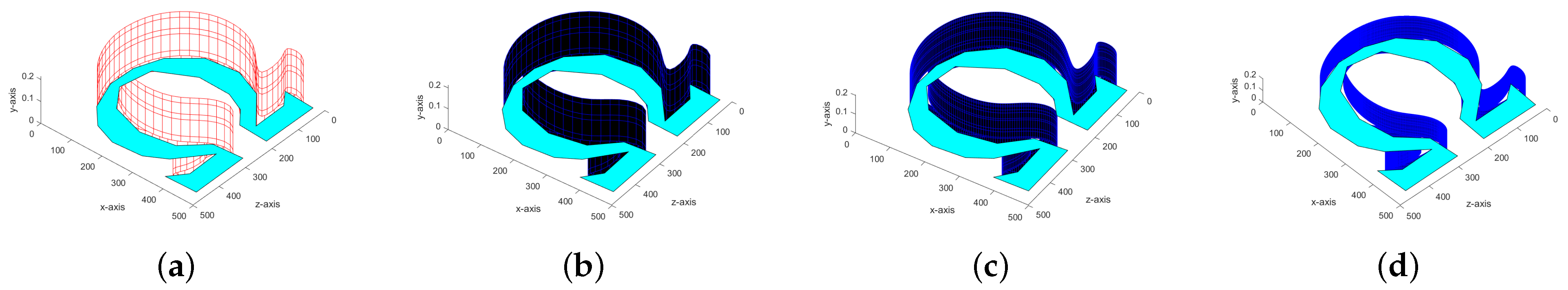
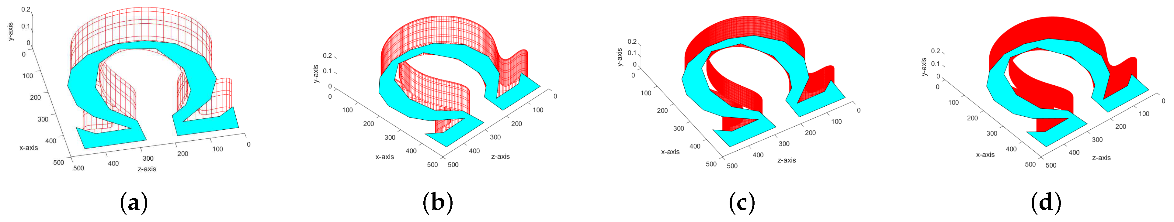
Tensor product subdivision schemes are powerful tools for generating smooth surfaces. One of the key advantages of tensor product subdivision schemes is their ability to generate regular surfaces. These surfaces are useful in a wide range of applications, including computer-aided geometric design and animation. The 4-point tensor product quaternary scheme is a specific type of tensor product subdivision scheme. The Figure 7 and Figure 8 show regular surfaces generated by the 4-point tensor product quaternary scheme using different parametric values. From these figures, we conclude that the proposed schemes can generate regular surfaces from their initial control structures.

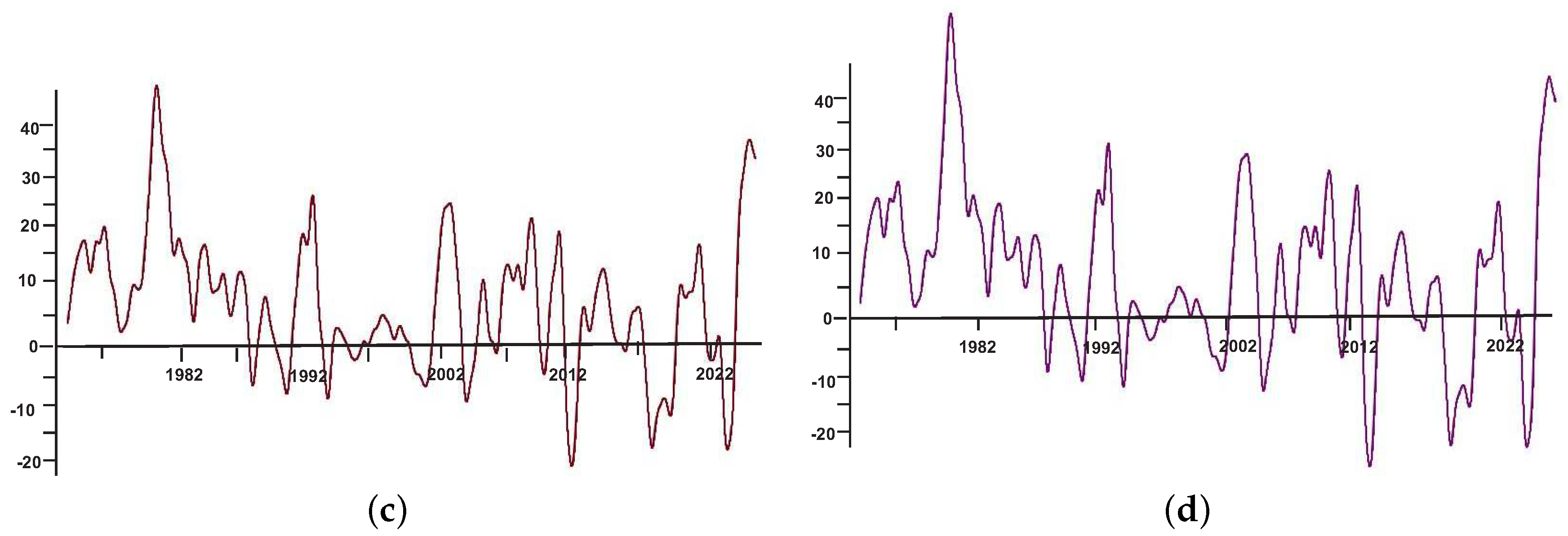
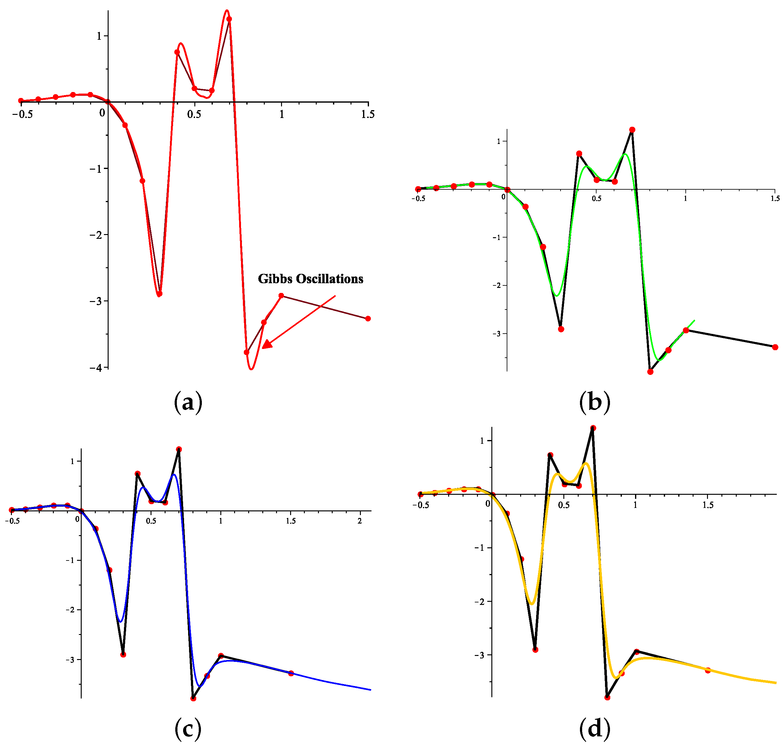
Example 1.

We use real data from the Australian Bureau of Statistics (www.abs.gov.au) (CPI) data set for our numerical experiment. Yearly and quarterly fluctuations in the price of automotive fuel from the years 1973 to 2022 are displayed against annual movement $(\%)$ in the graph.

Example 2.

In this numerical experiment, we perform a comparison between our proposed subdivision scheme and the existing linear subdivision scheme [1] by taking the following discontinuous function.

$$\begin{array}{c}\hfill \hslash \left(x\right)=\left\{\begin{array}{cc}x{(x+1)}^6,& ifx\in [-0.5,0.3]\\ sin\left(2\pi x\right)-2-cos\left(0.6\pi \right),& ifx\in [0.3,0.7]\\ x^4+x.& ifx\in [0.7,1]\end{array}\right.\end{array}$$

The original function $\hslash \left(x\right)$ is plotted in a solid black line. Red circles show the initial control points. Here we see that the Gibbs effects and unwanted high oscillations due to the presence of a jump discontinuity are reduced with our proposed subdivision scheme.

Example 3.

In this numerical experiment, we present some geometric shapes generated by some members of the family of schemes. Here RL stands for refinement/subdivision level.

9. Conclusions

We presented a simple method for constructing a class of approximating n-ary symmetric subdivision schemes based on well-known Lagrange’s and B-spline polynomials in this paper. This paper also illustrated quadratic and cubic spline curves with a local shape parameter. The basis functions construct curves that satisfy some important properties of quadratic and cubic B-splines, such as convex hull, shape-preserving property, and $G^1$ and $G^2$ geometric continuities. Several examples are given to demonstrate how the suggested schemes give geometric designers a better option for creating smooth geometric models that meet their needs. A comparison with some existing binary, ternary, and quaternary schemes is also given. We have demonstrated that several previously proposed schemes, including Chaikin’s scheme, belong to our proposed class of subdivision schemes. Members of the proposed classes also reduce or eliminate unattractive artifacts and eliminate the Gibbs-like phenomenon from the limit curves. Figure 6a illustrates the Gibbs oscillations, whereas Figure 6b–d, depicting our proposed schemes, show no signs of oscillations.

References

1. Dyn, N.; Floater, M.; Hormann, K. A C2 four-point subdivision scheme with fourth order accuracy and its extensions. In Proceedings of the International Conference on Mathematical Methods for Curves and Surfaces, Tromsø, Norway; 2005; pp. 145–156. [Google Scholar]
2. Ko, K.P.; Lee, B.G.; Yoon, G.J. A ternary 4-point approximating subdivision scheme. Appl. Math. Comput. 2007, 190, 1563–1573. [Google Scholar] [CrossRef]
3. Hussain, S.M.; Ur Rehman, A.; Baleanu, D.; Nisar, K.S.; Ghaffar, A.; Karim, S.A.A. Generalized 5-point approximating subdivision scheme of varying arity. Mathematics 2020, 8, 474. [Google Scholar] [CrossRef]
4. Rehan, K.; Siddiqi, S.S. A family of ternary subdivision schemes for curves. Appl. Math. Comput. 2015, 270, 114–123. [Google Scholar] [CrossRef]
5. Mustafa, G.; Khan, F.; Ghaffar, A. The m-point approximating subdivision scheme. Lobachevskii J. Math. 2009, 30, 138–145. [Google Scholar] [CrossRef]
6. Hameed, R.; Mustafa, G.; Hameed, R.; Younis, J.; Abd El Salam, M.A. Modeling of curves by a design-control approximating refinement scheme. Arab. J. Basic Appl. Sci. 2023, 30, 164–178. [Google Scholar] [CrossRef]
7. Conti, C.; Romani, L. Dual univariate m-ary subdivision schemes of de Rham-type. J. Math. Anal. Appl. 2013, 407, 443–456. [Google Scholar] [CrossRef]
8. Zhang, Z.; Zheng, H.; Zhou, J. Convergence analysis of Hermite subdivision schemes of any arity. Appl. Numer. Math. 2023, 183, 279–300. [Google Scholar] [CrossRef]
9. Wang, X.; Ma, W. An extended tuned subdivision scheme with optimal convergence for isogeometric analysis. Comput.-Aided Des. 2023, 103544. [Google Scholar] [CrossRef]
10. Nawaz, A.; Ghaffar, A.; Khan, F.; Karim, S.A.A. A new 7-point quaternary approximating subdivision scheme. In Intelligent Systems Modeling and Simulation II; Springer: Cham, Switzerland, 2022; Volume 444, pp. 545–566. [Google Scholar]
11. Zouaoui, S.; Amat, S.; Busquier, S.; Legaz, M.J. Some new n-point ternary subdivision schemes without the gibbs phenomenon. Mathematics 2022, 10, 2674. [Google Scholar] [CrossRef]
12. Iqbal, M.; Abdul Karim, S.A.; Shafie, A.; Sarfraz, M. Convexity preservation of the ternary 6-point interpolating subdivision scheme. In Towards Intelligent Systems Modeling and Simulation; Springer: Cham, Switzerland, 2021; Volume 383, pp. 1–23. [Google Scholar]
13. Amat, S.; Choutri, A.; Ruiz, J.; Zouaoui, S. On a nonlinear 4-point ternary and non-interpolatory subdivision scheme eliminating the Gibbs phenomenon. Appl. Math. Comput. 2018, 320, 16–26. [Google Scholar] [CrossRef]
14. Zhou, J.; Zheng, H.; Zhang, B. Gibbs phenomenon for p-ary subdivision schemes. J. Inequalities Appl. 2019, 2019, 48. [Google Scholar] [CrossRef]
15. Liu, Y.; Shou, H.; Ji, K. Review of subdivision schemes and their anpplications. Recent Patents Eng. 2022, 16, 50–62. [Google Scholar]
16. Schulze, R.; Heil, U.; Gross, D.; Bruellmann, D.D.; Dranischnikow, E.; Schwanecke, U.; Schoemer, E. Artefacts in CBCT: A review. Dentomaxillofac. Radiol. 2011, 40, 265–273. [Google Scholar] [CrossRef] [PubMed]
17. Lyu, J.; Akhavan, J.; Manoochehri, S. Image-based dataset of artifact surfaces fabricated by additive manufacturing with applications in machine learning. Data Brief 2022, 41, 107852. [Google Scholar] [CrossRef]
18. Karlen, W.; Ansermino, J.M.; Dumont, G. Adaptive pulse segmentation and artifact detection in photoplethysmography for mobile applications. In Proceedings of the 2012 Annual International Conference of the IEEE Engineering in Medicine and Biology Society, San Diego, CA, USA, 28 August–1 September 2012; pp. 3131–3134. [Google Scholar]
19. Gaêta-Araujo, H.; Leandro Nascimento, E.H.; Cavalcante Fontenele, R.; Maseti Mancini, A.X.; Queiroz Freitas, D.; Oliveira-Santos, C. Magnitude of beam-hardening artifacts produced by gutta-percha and metal posts on conebeam computed tomography with varying tube current. Imaging Sci. Dent. 2020, 50, 1–7. [Google Scholar] [CrossRef]
20. Barsky, B.A. The Beta Spline: A Local Representation Based on Shape Parameters and Fundamental Geometric Measure. Ph.D. Thesis, University of Utah, Salt Lake City, UT, USA, 1981. [Google Scholar]
21. Costantini, P. Curve and surface construction using variable degree polynomial splines. Comput. Aided Geom. Des. 2000, 17, 419–446. [Google Scholar] [CrossRef]
22. Farouki, R.T.; Manni, C.; Sestini, A. Shape preserving interpolation by G1 and G2 PH quintic splines. IMA J. Numer. Anal. 2003, 23, 175–195. [Google Scholar] [CrossRef]
23. Xu, G.; Wang, G. Extensions of uniform cubic B-spline curve with local shape parameters. Jisuanji Yanjiu yu Fazhan/Computer Res. Dev. 2007, 44, 1032–1037. [Google Scholar] [CrossRef]
24. Han, X.; Yang, J. Piecewise polynomial curves with normalized derivatives. J. Comput. Appl. Math. 2021, 388, 113290. [Google Scholar] [CrossRef]
25. Cao, J.; Wang, G. Structure of uniform B-spline curves with parameters. Prog. Nat. Sci. 2008, 18, 303–308. [Google Scholar] [CrossRef]
26. Rabbath, C.; Corriveau, D. A comparison of piecewise cubic Hermite interpolating polynomials, cubic splines and piecewise linear functions for the approximation of projectile aerodynamics. Def. Technol. 2019, 15, 741–757. [Google Scholar] [CrossRef]
27. Aspert, N. Non-Linear Subdivision of Univariate Signals and Discrete Surfaces; Technical Report; EPFL: Lausanne, Switzerland, 2003. [Google Scholar]
28. Salomon, D. Computer Graphics and Geometric Modeling; Springer: London, UK, 1999. [Google Scholar]
29. Hameed, R.; Mustafa, G.; Majeed, R. Variations in 2D and 3D models by a new family of subdivision schemes and algorithms for its analysis. Math. Probl. Eng. 2022, 2022, 3661307. [Google Scholar] [CrossRef]
30. Siddiqi, S.S.; Ahmad, N. A C6 approximating subdivision scheme. Appl. Math. Lett. 2008, 21, 722–728. [Google Scholar] [CrossRef]
31. Sabin, M.A.; Augsdörfer, U.H.; Dodgson, N.A. Artifacts in box-spline surfaces. In Proceedings of the Mathematics of Surfaces XI, Lecture Notes in Computer Science. Loughborough, UK, 5–7 September 2005; Springer: Berlin/Heidelberg, Germany, 2005; Volume 3604, pp. 350–363. [Google Scholar] [CrossRef]
32. Hormann, K. Subdivision schemes for geometric modeling a hands-on tutorial. Dolomites Res. 2012, 5. Available online: http://drna.padovauniversitypress.it/volume/5 (accessed on 19 May 2023).
33. Han, X. Piecewise quartic polynomial curves with a local shape parameter. J. Comput. Appl. Math. 2006, 195, 34–45. [Google Scholar] [CrossRef]
34. Siddiqi, S.S.; Ahmad, N. An approximating C4 stationary subdivision scheme. Eur. J. Sci. Res. 2006, 15, 97–102. [Google Scholar]
35. Asghar, M.; Mustafa, G. Family of a-ary univariate subdivision schemes generated by Laurent polynomial. Math. Probl. Eng. 2018, 2018, 7824279. [Google Scholar] [CrossRef]
36. Zheng, H.; Huang, S.; Guo, F.; Peng, G. Integer-point binary approximating subdivision schemes. J. Inf. Comput. Sci. 2014, 11, 3387–3398. [Google Scholar] [CrossRef]
37. Zheng, H.; Hu, M.; Peng, G. P-ary subdivision generalizing B-splines. In Proceedings of the 2008 International Conference on Computer Science and Software Engineering (CSSE 2008), Wuhan, China, 12–14 December 2008; pp. 214–218. [Google Scholar] [CrossRef]
38. Siddiqi, S.S.; Ahmad, N. A new three-point approximating C2 subdivision scheme. Appl. Math. Lett. 2007, 20, 707–711. [Google Scholar] [CrossRef]
39. Hormann, K.; Sabin, M.A. A family of subdivision schemes with cubic precision. Comput. Aided Geom. Des. 2008, 25, 41–52. [Google Scholar] [CrossRef]
40. Hassan, M.F.; Dodgson, N.A. Ternary and three-point univariate subdivision schemes. In Curve and Surface Fitting: Saint-Malo; Nashboro Press: Brentwood, TN, USA, 2003; pp. 199–208. [Google Scholar]
41. Chaikin, G.M. An algorithm for high-speed curve generation. Comput. Graph. Image Process. 1974, 3, 346–349. [Google Scholar] [CrossRef]
42. Siddiqi, S.S.; Rehan, K. Modified form of binary and ternary 3-point subdivision schemes. Appl. Math. Comput. 2010, 216, 970–982. [Google Scholar] [CrossRef]
43. Daniel, S.; Shunmugaraj, P. Three point stationary and non-stationary subdivision schemes. In Proceedings of the 3rd International Conference on Geometric Modeling and Imaging: Modern Techniques and Applications (GMAI 2008), London, UK, 9–11 July 2008; pp. 3–8. [Google Scholar] [CrossRef]
44. Ghaffar, A.; Mustafa, G.; Qin, K. Unification and application of 3-point approximating subdivision schemes of varying arity. Open J. Appl. Sci. 2012, 02, 48–52. [Google Scholar] [CrossRef]
45. Ghaffar, A.; Mustafa, G.; Qin, K. The 4-point α-ary approximating subdivision scheme. Open J. Appl. Sci. 2013, 3, 106–111. [Google Scholar] [CrossRef]
46. Ghaffar, A.; Mustafa, G. A family of even-point ternary approximating schemes. ISRN Appl. Math. 2012, 2012, 197383. [Google Scholar] [CrossRef]
47. Zheng, H.; Hu, M.; Peng, G.; Zheng, H.; Wolff, T. Ternary even symmetric 2n-point subdivision. In Proceedings of the 2009 International Conference on Computational Intelligence and Software Engineering (CiSE 2009), Wuhan, China, 11–13 December 2009; Volume 234, pp. 1–59. [Google Scholar] [CrossRef]
48. Siddiqi, S.S.; Younis, M. The m-point quaternary approximating subdivision schemes. Am. J. Comput. Math. 2013, 3, 6–10. [Google Scholar] [CrossRef]
49. Ko, K.P.Y.O. A quatnary approximating 4-point subdivision scheme. J. Korea Soc. Ind. Appl. Math. 2009, 13, 307–314. [Google Scholar]
50. Mustafa, G.; Khan, F. A new 4-point C3 quaternary approximating subdivision scheme. Abstr. Appl. Anal. 2009, 2009, 301967. [Google Scholar] [CrossRef]
51. Mustafa, G.; Asghar, M.; Ali, S.; Qamar, A.; BaoLiu, J. The family of multiparameter quaternary subdivision schemes. J. Math. 2021, 2021, 4732464. [Google Scholar] [CrossRef]
52. Dubuc, S. Interpolation through an iterative scheme. J. Math. Anal. Appl. 1986, 114, 185–204. [Google Scholar] [CrossRef]
Figure 1. Graphs of the basic limit functions of the proposed 4-point scheme at different values of the parameters. (a) A 4-point binary scheme) (18) ( α = 0.625 , 0.3125 , 0.0625 ). (b) A 4-point ternary scheme (19) ( α = 0.2 , 0.5 , 0.5 ). (c) A 4-point quaternary scheme (20) ( α = 0.078 , 0.3125 , 0.5 ). (d) A 4-point quinary scheme (21) ( α = 0.01 , 0.05 , 0.65 ).
Symmetry 15 01620 g001
Figure 2. A 3-point binary scheme  α = 1 5 , 1 9 , 0 , 1 9 , 1 8 , 1 7 . This figure presents the effect of a parameter on magnitudes of artifact plotted versus the number of control points in the limit curves of the schemes (11). The artifact decreases with the decrease of the value of parameter.
Symmetry 15 01620 g002
Figure 3. A 4-point binary scheme  α = 5 16 , 2 16 , 0 , 1 50 . This figure presents the effect of parameter on magnitudes of artifact corresponding to the number of control points in the limit curves of the schemes. The artifact decreases with the decrease of the value of parameter.
Symmetry 15 01620 g003
Figure 4. Influence of the parameter on: (a) quadratic (33) and (b) cubic (35) spline shapes.
Symmetry 15 01620 g004
Figure 5. Red solid lines show the Automotive Fuel CPI series. Coloured lines show the curve fitted by our subdivision scheme after three refinement steps. (a) Automotive fuel CPI series. (b) A 4-point binary scheme. (c) A 4-point ternary scheme. (d) A 4-point quaternary scheme.
Symmetry 15 01620 g005aSymmetry 15 01620 g005b
Figure 6. Initial control points are shown by red bullets. Black solid lines indicate the original control polygons. Coloured lines show the fitted curves by 4-point (18), (19) and (20) schemes in (bd). (a) 4-point scheme [52]. (b) 4-point proposed binary scheme ( α = 0.5626 ). (c) 4-point proposed ternary scheme ( α = 0.31 ). (d) 4-point proposed quaternary scheme ( α = 0.01 ).
Symmetry 15 01620 g006
Figure 7. The surface generated by the tensor product of the 4-point quaternary scheme at different refinement levels at parametric value  α = 13 46 . (a) First RL. (b) Second RL. (c) Third RL. (d) Fourth RL.
Symmetry 15 01620 g007
Figure 8. The surface generated by the tensor product of the 4-point quaternary scheme at different refinement levels at parametric value  α = 35 64 . (a) First RL. (b) Second RL. (c) Third RL. (d) Fourth RL.
Symmetry 15 01620 g008