New Three Wave and Periodic Solutions for the Nonlinear (2+1)-Dimensional Burgers Equations

Abstract

This research paper is about the new three wave, periodic wave and other analytical wave solutions of (2+1)-Dimensional Burgers equations by utilizing Hirota bilinear and extended sinh-Gordon equation expansion (EShGEE) schemes. Achieved solutions are verified and demonstrated by different plots with the use of Mathematica 11.01 software. Some of the achieved solutions are also described graphically by two-dimensional, three-dimensional and contour plots. The gained solutions are helpful for the future study of concerned models. Finally, these two schemes are simple, fruitful and reliable to handle the nonlinear PDEs.

1. Introduction

Symmetry is used in real life to simplify calculations and solve problems more easily. Symmetry also offers human beings an additional extension to their capabilities. Applications of symmetry are determining the orbital overlap for molecular orbital, understanding the spectroscopic properties of molecules and identifying chiral molecular species, etc. Symmetry is a frequently recurring theme in mathematics, nature, science, etc. In mathematics, its most familiar manifestation appears in geometry [1,2].

The nonlinear partial differential equations (NLPDEs) arise in various types of physical problems such as fluid dynamics, plasma physics, quantum field theory, etc. The system of nonlinear partial differential Equations has been observed in chemical, biological, engineering and other areas of applied sciences. A lot of research has been performed in these areas to find the numerical and analytical results of NLPDEs. Various schemes have been developed for this purpose. For example, the auxiliary rational method [3], Kudryashov technique [4], two variable $(G^{\prime }/G,1/G)$-expansion technique [5], mapping method [6], generalized auxiliary equation method [7], modified F-expansion technique [8], unified method [9], modified extended tanh expansion method [10], modified simplest equation technique [11], extended Jacobi elliptic function scheme [12], He’s semi-inverse and Riccati equation mapping schemes [13], the $tanh\text{-}coth$ technique [14], exp$(-\phi (\mu \left)\right)$-expansion scheme [15], etc.

Except for these schemes, there are two other simple, useful, and significant schemes: the Hirota bilinear scheme and the extended sinh-Gordon equation expansion scheme. The Hirota bilinear method can be used to search for new integrable evolution equations. Solutions obtained through the Hirota bilinear method have distinct structures, but all of them have emerged under the banner of the same scheme. This scheme solves solutions without setting solutions, and calculates transformations without making logarithmic transformations. The extended sinh-Gordon equation expansion scheme is a powerful scheme for solving non-linear partial differential equations. It is widely used in various areas of physics, engineering and mathematics. In the literature, there are many applications of these two schemes. For example, by using the Hirota bilinear method three-wave solutions of the (3+1)-dimensional Boiti–Leon–Manna–Pempinelli model have been gained [16], and new periodic wave solutions of the (2+1)-dimensional breaking soliton equation [17]. Some optical solitons of the new Hamiltonian Amplitude model have been achieved by applying the extended sinh-Gordon equation expansion scheme in [18]. New types of optical wave solutions of the Biswas–Arshed equation have been gained by the EShGEE scheme [19].

Our study model is a nonlinear (2+1)-dimensional Burgers equations given as [20]:

$$\begin{array}{c}\hfill g_t={\mathit{gg}}_y+{\mathit{ahg}}_x+{\mathit{bg}}_{yy}+{\mathit{abg}}_{xx}.\\ \hfill g_x=h_y.\end{array}$$

(1)

where g = g(x,y,t) and h = h(x,y,t) denote the wave profiles, while a and b are the constants. Equation (1) has been studied by many researchers, e.g., Solitary, periodic and rational wave solutions have been gained by utilizing the new Riccati equation rational expansion method. Lump, rogue wave and interaction wave solutions have been gained by Hirota bilinear scheme [21]. Non-trivial wave solutions are achieved with by utilizing auxiliary equation method [22].

The main motivation of this research is to explore the new three wave, periodic wave and other analytical solitons of the non-linear (2+1)-dimensional Burgers equations based on the Hirota bilinear scheme and the extended sinh-Gordon equation expansion scheme. Our research model’s Burgers equations are a fundamental partial differential equation from fluid mechanics. They occur in many fields of applied mathematics such as modeling of gas dynamics, traffic flow, etc. The schemes that are used in this research have never been applied to this model before, and the obtained results are newer than the existing results of this model in the literature. The diverse graphical analyses for the presented solutions show that the solutions are reliable for the further development in the model, and also in other areas of mathematical physics and engineering.

This paper is organized as follows. In Section 1; we brief the Hirota bilinear scheme, we apply the Hirota bilinear scheme to obtain the new periodic and three wave solutions to the (2+1)-dimensional Burgers equations. In Section 3; we give the details of the extended sinh-Gordon equation expansion scheme, and we apply the extended sinh-Gordon scheme to find out the exact solutions. In Section we apply the EShGEE scheme to gain the analytical wave solutions to the (2+1)-dimensional Burgers equations. In Section 4; we demonstrate some solutions with the help of different kinds of plots. In Section 5: we give the, conclusion.

2. Hirota Bilinear Scheme and Its Application

2.1. The Bilinear Form Polynomials

According to the [23], let us assume $\zeta =\zeta (x_1,x_2,\dots ,x_n)$ is a $C^{\infty }$ function is shown below

$${\mathsf{{\rm Y}}}_{n_1{x}_1,\dots ,n_j{x}_j}\left(\zeta \right)\equiv {\mathsf{{\rm Y}}}_{n_1,\dots ,n_j}\left({\zeta }_{s_1{x}_1,\dots ,s_j{x}_j}\right)=e^{-\zeta }{\partial }_{x_1}^{n_1}\dots {\partial }_{x_j}^{n_j}{e}^{\zeta },$$

(2)

along binary Bell polynomials (BBPs) as below

$${\zeta }_{s_1{x}_1,\dots ,s_j{x}_j}={\partial }_{x_1}^{s_1}\dots {\partial }_{x_j}^{s_j}\zeta ,{\zeta }_{0x_i}\equiv \zeta ,s_1=0,\dots ,n_1;\dots ;s_j=0,\dots ,n_j,$$

and we have

$${\mathsf{{\rm Y}}}_1\left(\zeta \right)={\zeta }_x,{\mathsf{{\rm Y}}}_2\left(\zeta \right)={\zeta }_{2x}+{\zeta }_x^2,{\mathsf{{\rm Y}}}_3\left(\zeta \right)={\zeta }_{3x}+3{\zeta }_x{\zeta }_{2x}+{\zeta }_x^3,{\dots }_{,}\zeta =\zeta (x,t),$$

$${\mathsf{{\rm Y}}}_{x,t}\left(\zeta \right)={\zeta }_{x,t}+{\zeta }_x{\zeta }_t,{\mathsf{{\rm Y}}}_{2x,t}\left(\zeta \right)={\zeta }_{2x,t}+{\zeta }_{2x}{\zeta }_t+2{\zeta }_{x,t}{\zeta }_x+{\zeta }_x^2{\zeta }_t,{\dots }_{.}$$

(3)

The multi-D BBPs may be represented as in the below

$${\mathsf{\Sigma }}_{n_1{x}_1,\dots ,n_j{x}_j}(A,B)={\left.{\mathsf{{\rm Y}}}_{n_1,\dots ,n_j}\left(\zeta \right)\right|}_{{\zeta }_{s_1{x}_1,\dots ,s_j{x}_j}=\left\{\begin{array}{cc}{A}_{s_1{x}_1,\dots ,s_j{x}_j},\hfill & s_1+s_2+\dots +s_j,\mathrm{is}\mathrm{odd}\hfill \\ B_{s_1{x}_1,\dots ,s_j{x}_j},\hfill & s_1+s_2+\dots +s_j,\mathrm{is}\mathrm{even}.\hfill \end{array}\right.}$$

(4)

We have the conditions given as follows:

$${\mathsf{\Sigma }}_x\left(A\right)=A_x,{\mathsf{\Sigma }}_{2x}(A,B)=B_{2x}+A_x^2,{\mathsf{\Sigma }}_{x,t}(A,B)=B_{x,t}+A_x{A}_t,{\dots }_{.}$$

(5)

Proposition 1.

Consider

$$A=ln(\mathsf{\Theta }/\mathsf{\Delta }),B=ln\left(\mathsf{\Theta }\mathsf{\Delta }\right),$$

(6)

then the connection between BBPs and Hirota D-operator can be written the below

$${\left.{\mathsf{\Sigma }}_{n_1{x}_1,\dots ,n_j{x}_j}(A,B)\right|}_{A=ln(\mathsf{\Theta }/\mathsf{\Delta }),B=ln\left(\mathsf{\Theta }\mathsf{\Delta }\right)}={\left(\mathsf{\Theta }\mathsf{\Delta }\right)}^{-1}{D}_{x_1}^{n_1}\dots D_{x_j}^{n_j}\mathsf{\Theta }\mathsf{\Delta },$$

(7)

with Hirota formula

$$\prod _{i=1}^j{D}_{x_i}^{n_i}g.\eta ={\left.\prod _{i=1}^j{\left(\frac{\partial }{\partial x_i}-\frac{\partial }{\partial x_i^{\prime }}\right)}^{n_i}\mathsf{\Theta }(x_1,\dots ,x_j)\mathsf{\Delta }(x_1^{\prime },\dots ,x_j^{\prime })\right|}_{x_1=x_1^{\prime },\dots ,x_j=x_j^{\prime }}.$$

(8)

Proposition 2.

Take

$$\mathsf{\Xi }\left(A\right)=\sum _i{\delta }_i{\mathfrak{P}}_{s_1{x}_1,\dots ,s_j{x}_j}=0,A=ln(\mathsf{\Theta }/\mathsf{\Delta }),B=ln\left(\mathsf{\Theta }\mathsf{\Delta }\right),$$

(9)

we have

$$\left\{\begin{array}{c}\sum _i{\delta }_{1i}{\mathsf{{\rm Y}}}_{n_1{x}_1,\dots ,n_j{x}_j}(A,B)=0,\hfill \\ \sum _i{\delta }_{1i}{\mathsf{{\rm Y}}}_{s_1{x}_1,\dots ,s_j{x}_j}(A,B)=0,\hfill \end{array}\right.$$

(10)

with below conditions

$$\mathfrak{R}({\aleph }^{\prime },\aleph )=\mathfrak{R}\left({\aleph }^{\prime }\right)-\mathfrak{R}(\aleph )=\mathfrak{R}(B+A)-\mathfrak{R}(B-A)=0.$$

(11)

The generalized Bell polynomials ${\mathsf{{\rm Y}}}_{n_1{x}_1,\dots ,n_j{x}_j}\left(\xi \right)$ is

$${\left(\mathsf{\Theta }\mathsf{\Delta }\right)}^{-1}{D}_{x_1}^{n_1}\dots D_{x_j}^{n_j}\mathsf{\Theta }\mathsf{\Delta }={\left.{\mathsf{\Sigma }}_{n_1{x}_1,\dots ,n_j{x}_j}(A,B)\right|}_{A=ln(\mathsf{\Theta }/\mathsf{\Delta }),B=ln\left(\mathsf{\Theta }\mathsf{\Delta }\right)}$$

(12)

$$={\left.{\mathsf{\Sigma }}_{n_1{x}_1,\dots ,n_j{x}_j}(A,A+\gamma )\right|}_{A=ln(\mathsf{\Theta }/\mathsf{\Delta }),\gamma =ln\left(\mathsf{\Theta }\mathsf{\Delta }\right)}$$

$$=\sum _{k_1}^{n_1}\dots \sum _{k_j}^{n_j}\prod _{i=1}^j\left(\begin{array}{c}{n}_i\\ k_i\end{array}\right){\mathfrak{P}}_{k_1{x}_1,\dots ,k_j{x}_j}\left(\gamma \right){\mathsf{{\rm Y}}}_{(n_1-k_1)x_1,\dots ,(n_j-k_j)x_j}\left(A\right).$$

The Cole-Hopf transformation becomes

$${\mathsf{{\rm Y}}}_{k_1{x}_1,\dots ,k_j{x}_j}(A=ln\left(f\right))=\frac{f_{n_1{x}_1,\dots ,n_j{x}_j}}{f},$$

(13)

$${\left.{\left(\mathsf{\Theta }\mathsf{\Delta }\right)}^{-1}{D}_{x_1}^{n_1}\dots D_{x_j}^{n_j}\mathsf{\Theta }\mathsf{\Delta }\right|}_{\mathsf{\Delta }=exp(\gamma /2),\mathsf{\Theta }/\mathsf{\Delta }=f}$$

(14)

$$=f^{-1}\sum _{k_1}^{n_1}\dots \sum _{k_j}^{n_j}\prod _{d=1}^j\left(\begin{array}{c}{n}_d\\ k_d\end{array}\right){\mathfrak{P}}_{k_1{x}_1,\dots ,k_d{x}_d}\left(\gamma \right)f_{(n_1-k_1)x_1,\dots ,(n_d-k_d)x_d},$$

with

$${\mathsf{{\rm Y}}}_t\left(A\right)=\frac{f_t}{f},{\mathsf{{\rm Y}}}_{2x}(A,\beta )={\gamma }_{2x}+\frac{f_{2x}}{f},{\mathsf{{\rm Y}}}_{2x,y}(A,B)=\frac{{\gamma }_{2x}{f}_y}{f}+\frac{2{\gamma }_{x,y}{f}_x}{f}+\frac{f_{2x,y}}{f}.$$

(15)

Let us assume the following transformations to obtain the Hirota bilinear form of Equation (1).

$$g(x,y,t)=2b{(lnf)}_y+g_0,h(x,y,t)=2b{(lnf)}_x+h_0.$$

(16)

By using Equation (16) into Equations (1), we obtain

$$2a{b}^2{f}_{\mathrm{xx}}{f}_y-2a{b}^{2}f{f}_{\mathrm{xxy}}+2ab{h}_0{f}_x{f}_y-2abf{h}_0{f}_{\mathrm{xy}}+2b^2{f}_y{f}_{\mathrm{yy}}-2b^{2}f{f}_{\mathrm{yyy}}+2b{g}_0{f}_y^2-2bf{g}_0{f}_{\mathrm{yy}}-2b{f}_t{f}_y+2bf{f}_{\mathrm{yt}}=0.$$

(17)

2.2. New Three-Wave Solutions

We assume the transformation given as to gain the new three-wave results [16].

$$f(x,y,t)={\kappa }_2{e}^{a_{1}x+b_{1}y+d_{1}t}+{\kappa }_{3}sin\left(a_{3}x+b_{3}y+d_{3}t\right)+{\kappa }_{1}cos\left(a_{2}x+b_{2}y+d_{2}t\right)+e^{-\left(a_{1}x+b_{1}y+d_{1}t\right)}$$

(18)

Substituting Equation (18) into Equation (17), we gain a system of equations by summing up coefficients of every power of $e^{a_{1}x+b_{1}y+d_{1}t}$, $e^{-\left(a_{1}x+b_{1}y+d_{1}t\right)}$, $sin\left(a_{3}x+b_{3}y+d_{3}t\right)$ and $cos\left(a_{2}x+b_{2}y+d_{2}t\right)$ and putting them equal to 0. We gain the solution sets by solving the system given as follows:

Set 1:

$$\begin{array}{c}\{a_2=-\frac{}{\sqrt{a}},a_3=-\frac{R}{\sqrt{a}},d_1=a{a}_1{h}_0+b_1{g}_0,d_2=b_2{g}_0-\sqrt{a}{h}_0\sqrt{-a{a}_1^2-b_1^2-b_2^2},\hfill \\ \hfill d_3=b_3{g}_0-\sqrt{a}{h}_{0}R,R=\sqrt{-a{a}_1^2-b_1^2-b_3^2},H=\sqrt{-a{a}_1^2-b_1^2-b_2^2}\}\end{array}$$

(19)

$$\begin{array}{c}\hfill g(x,y,t)=2b\left(\right(b_1(-exp(-t(a{a}_1{h}_0+b_1{g}_0)-a_{1}x-b_{1}y))+b_1{\kappa }_{2}exp(t(a{a}_1{h}_0+b_1{g}_0)+a_{1}x+b_{1}y)\\ \hfill -b_2{\kappa }_{1}sin(t(b_2{g}_0-\sqrt{a}{h}_{0}H)-\frac{xH}{\sqrt{a}}+b_{2}y)+b_3{\kappa }_{3}cos(t(b_3{g}_0-\sqrt{a}{h}_{0}R)-\frac{xR}{\sqrt{a}}+b_{3}y))/\\ \hfill (exp(-t(a{a}_1{h}_0+b_1{g}_0)-a_{1}x-b_{1}y)+{\kappa }_{2}exp(t(a{a}_1{h}_0+b_1{g}_0)+a_{1}x+b_{1}y)+{\kappa }_{3}sin(t(b_3{g}_0-\sqrt{a}{h}_{0}R)\\ \hfill -\frac{xR}{\sqrt{a}}+b_{3}y)+{\kappa }_{1}cos(t(b_2{g}_0-\sqrt{a}{h}_{0}H)-\frac{xH}{\sqrt{a}}+b_{2}y)\left)\right)+g_0\end{array}$$

(20)

$$\begin{array}{c}\hfill h(x,y,t)=2b\left(\right(a_1(-exp(-t(a{a}_1{h}_0+b_1{g}_0)-a_{1}x-b_{1}y))+a_1{\kappa }_{2}exp(t(a{a}_1{h}_0+b_1{g}_0)+a_{1}x+b_{1}y)\\ \hfill +\frac{{\kappa }_{1}Hsin(t(b_2{g}_0-\sqrt{a}{h}_{0}H)-\frac{xH}{\sqrt{a}}+b_{2}y)}{\sqrt{a}}-\frac{{\kappa }_{3}Rcos(t(b_3{g}_0-\sqrt{a}{h}_{0}R)-\frac{xR}{\sqrt{a}}+b_{3}y)}{\sqrt{a}})/\\ \hfill (exp(-t(a{a}_1{h}_0+b_1{g}_0)-a_{1}x-b_{1}y)+{\kappa }_{2}exp(t(a{a}_1{h}_0+b_1{g}_0)+a_{1}x+b_{1}y)\\ \hfill +{\kappa }_{3}sin(t(b_3{g}_0-\sqrt{a}{h}_{0}R)-\frac{xR}{\sqrt{a}}+b_{3}y)+{\kappa }_{1}cos(t(b_2{g}_0-\sqrt{a}{h}_{0}H)-\frac{xH}{\sqrt{a}}+b_{2}y)\left)\right)+h_0\end{array}$$

(21)

Set 2:

$$\begin{array}{c}\hfill \{a_2=-\frac{xH}{\sqrt{a}},a_3=\frac{R}{\sqrt{a}},d_1=a{a}_1{h}_0+b_1{g}_0,d_2=b_2{g}_0-\sqrt{a}{h}_{0}H,d_3=\sqrt{a}{h}_{0}R+b_3{g}_0,\\ \hfill H=\sqrt{-a{a}_1^2-b_1^2-b_2^2},R=\sqrt{-a{a}_1^2-b_1^2-b_3^2}\}\end{array}$$

(22)

$$\begin{array}{c}\hfill g(x,y,t)=2b\left(\right(b_1(-exp(-t(a{a}_1{h}_0+b_1{g}_0)-a_{1}x-b_{1}y))+b_1{\kappa }_{2}exp(t(a{a}_1{h}_0+b_1{g}_0)+a_{1}x+b_{1}y)-b_2{\kappa }_1\\ \hfill sin(t(b_2{g}_0-\sqrt{a}{h}_{0}H)-\frac{xH}{\sqrt{a}}+b_{2}y)+b_3{\kappa }_{3}cos(t(\sqrt{a}{h}_{0}R+b_3{g}_0)+\frac{xR}{\sqrt{a}}+b_{3}y))/\\ \hfill (exp(-t(a{a}_1{h}_0+b_1{g}_0)-a_{1}x-b_{1}y)+{\kappa }_{2}exp(t(a{a}_1{h}_0+b_1{g}_0)+a_{1}x+b_{1}y)+{\kappa }_{3}sin(t(\sqrt{a}{h}_{0}R+b_3{g}_0)\\ \hfill +\frac{xR}{\sqrt{a}}+b_{3}y)+{\kappa }_{1}cos(t(b_2{g}_0-\sqrt{a}{h}_{0}H)-\frac{xH}{\sqrt{a}}+b_{2}y)\left)\right)+g_0\end{array}$$

(23)

$$\begin{array}{c}\hfill h(x,y,t)=2b\left(\right(a_1(-exp(-t(a{a}_1{h}_0+b_1{g}_0)-a_{1}x-b_{1}y))+a_1{\kappa }_{2}exp(t(a{a}_1{h}_0+b_1{g}_0)+a_{1}x+b_{1}y)+\\ \hfill \frac{{\kappa }_{1}Hsin(t(b_2{g}_0-\sqrt{a}{h}_{0}H)-\frac{xH}{\sqrt{a}}+b_{2}y)}{\sqrt{a}}+\frac{{\kappa }_{3}Rcos(t(\sqrt{a}{h}_{0}R+b_3{g}_0)+\frac{xR}{\sqrt{a}}+b_{3}y)}{\sqrt{a}})/\\ \hfill (exp(-t(a{a}_1{h}_0+b_1{g}_0)-a_{1}x-b_{1}y)+{\kappa }_2{e}^{t(a{a}_1{h}_0+b_1{g}_0)+a_{1}x+b_{1}y}+{\kappa }_{3}sin(t(\sqrt{a}{h}_{0}R+b_3{g}_0)+\\ \hfill \frac{xR}{\sqrt{a}}+b_{3}y)+{\kappa }_{1}cos(t(b_2{g}_0-\sqrt{a}{h}_{0}H)-\frac{xH}{\sqrt{a}}+b_{2}y)\left)\right)+h_0\end{array}$$

(24)

Set 3:

$$\begin{array}{c}\{a_2=\frac{H}{\sqrt{a}},a_3=-\frac{R}{\sqrt{a}},d_1=a{a}_1{h}_0+b_1{g}_0,d_2=\sqrt{a}{h}_{0}H+b_2{g}_0,\hfill \\ d_3=b_3{g}_0-\sqrt{a}{h}_{0}R,H=\sqrt{-a{a}_1^2-b_1^2-b_2^2},R=\sqrt{-a{a}_1^2-b_1^2-b_3^2}\}\hfill \end{array}$$

(25)

$$\begin{array}{c}\hfill g(x,y,t)=2b\left(\right(b_1(-exp(-t(a{a}_1{h}_0+b_1{g}_0)-a_{1}x-b_{1}y))+b_1{\kappa }_{2}exp(t(a{a}_1{h}_0+b_1{g}_0)+a_{1}x+b_{1}y)-b_2{\kappa }_1\\ \hfill sin(t(\sqrt{a}{h}_{0}H+b_2{g}_0)+\frac{xH}{\sqrt{a}}+b_{2}y)+b_3{\kappa }_{3}cos(t(b_3{g}_0-\sqrt{a}{h}_{0}R)-\frac{xR}{\sqrt{a}}+b_{3}y))/\\ \hfill (exp(-t(a{a}_1{h}_0+b_1{g}_0)-a_{1}x-b_{1}y)+{\kappa }_{2}exp(t(a{a}_1{h}_0+b_1{g}_0)+a_{1}x+b_{1}y)\\ \hfill +{\kappa }_{3}sin(t(b_3{g}_0-\sqrt{a}{h}_{0}R)-\frac{xR}{\sqrt{a}}+b_{3}y)+{\kappa }_{1}cos(t(\sqrt{a}{h}_0\sqrt{-a{a}_1^2-b_1^2-b_2^2}+b_2{g}_0)\\ \hfill +\frac{xH}{\sqrt{a}}+b_{2}y\left)\right))+g_0\end{array}$$

(26)

$$\begin{array}{c}\hfill h(x,y,t)=2b\left(\right(a_1(-exp(-t(a{a}_1{h}_0+b_1{g}_0)-a_{1}x-b_{1}y))+a_1{\kappa }_{2}exp(t(a{a}_1{h}_0+b_1{g}_0)+a_{1}x+b_{1}y)\\ \hfill -\frac{{\kappa }_{1}Hsin(t(\sqrt{a}{h}_{0}H+b_2{g}_0)+\frac{xH}{\sqrt{a}}+b_{2}y)}{\sqrt{a}}-\frac{{\kappa }_{3}Rcos(t(b_3{g}_0-\sqrt{a}{h}_{0}R)-\frac{xR}{\sqrt{a}}+b_{3}y)}{\sqrt{a}})/\\ \hfill (exp(-t(a{a}_1{h}_0+b_1{g}_0)-a_{1}x-b_{1}y)+{\kappa }_{2}exp(t(a{a}_1{h}_0+b_1{g}_0)+a_{1}x+b_{1}y)+{\kappa }_{3}sin(t(b_3{g}_0-\sqrt{a}{h}_{0}R)\\ \hfill -\frac{xR}{\sqrt{a}}+b_{3}y)+{\kappa }_{1}cos(t(\sqrt{a}{h}_{0}H+b_2{g}_0)+\frac{xH}{\sqrt{a}}+b_{2}y)\left)\right)+h_0\end{array}$$

(27)

Set 4:

$$\begin{array}{c}\hfill \{a_2=\frac{}{\sqrt{a}},a_3=\frac{R}{\sqrt{a}},d_1=a{a}_1{h}_0+b_1{g}_0,d_2=\sqrt{a}{h}_{0}H+b_2{g}_0,d_3=\sqrt{a}{h}_{0}R+b_3{g}_0,\\ \hfill H=\sqrt{-a{a}_1^2-b_1^2-b_2^2},R=\sqrt{-a{a}_1^2-b_1^2-b_3^2}\}\end{array}$$

(28)

$$\begin{array}{c}\hfill g(x,y,t)=2b\left(\right(b_1(-exp(-t(a{a}_1{h}_0+b_1{g}_0)-a_{1}x-b_{1}y))+b_1{\kappa }_{2}exp(t(a{a}_1{h}_0+b_1{g}_0)+a_{1}x+b_{1}y)-b_2{\kappa }_1\\ \hfill sin(t(\sqrt{a}{h}_{0}H+b_2{g}_0)+\frac{xH}{\sqrt{a}}+b_{2}y)+b_3{\kappa }_{3}cos(t(\sqrt{a}{h}_{0}R+b_3{g}_0)+\frac{xR}{\sqrt{a}}+b_{3}y))/\\ \hfill (exp(-t(a{a}_1{h}_0+b_1{g}_0)-a_{1}x-b_{1}y)+{\kappa }_{2}exp(t(a{a}_1{h}_0+b_1{g}_0)+a_{1}x+b_{1}y)+{\kappa }_{3}sin(t(\sqrt{a}{h}_{0}R+b_3{g}_0)\\ \hfill +\frac{xR}{\sqrt{a}}+b_{3}y)+{\kappa }_{1}cos(t(\sqrt{a}{h}_{0}H+b_2{g}_0)+\frac{xH}{\sqrt{a}}+b_{2}y)\left)\right)+g_0\end{array}$$

(29)

$$\begin{array}{c}\hfill h(x,y,t)=2b\left(\right(a_1(-exp(-t(a{a}_1{h}_0+b_1{g}_0)-a_{1}x-b_{1}y))+a_1{\kappa }_{2}exp(t(a{a}_1{h}_0+b_1{g}_0)+a_{1}x+b_{1}y)\\ \hfill -\frac{{\kappa }_{1}Hsin(t(\sqrt{a}{h}_{0}H+b_2{g}_0)+\frac{xH}{\sqrt{a}}+b_{2}y)}{\sqrt{a}}+\frac{{\kappa }_{3}Rcos(t(\sqrt{a}{h}_{0}R+b_3{g}_0)+\frac{xR}{\sqrt{a}}+b_{3}y)}{\sqrt{a}})/\\ \hfill (exp(-t(a{a}_1{h}_0+b_1{g}_0)-a_{1}x-b_{1}y)+{\kappa }_{2}exp(t(a{a}_1{h}_0+b_1{g}_0)+a_{1}x+b_{1}y)+{\kappa }_{3}sin(t(\sqrt{a}{h}_{0}R+b_3{g}_0)+\\ \hfill \frac{xR}{\sqrt{a}}+b_{3}y)+{\kappa }_{1}cos(t(\sqrt{a}{h}_{0}H+b_2{g}_0)+\frac{xH}{\sqrt{a}}+b_{2}y)\left)\right)+h_0\end{array}$$

(30)

2.3. New Periodic Wave Solutions

Consider the following transformation [17]:

$$f(x,y,t)={\kappa }_1{e}^{a_{3}t+a_{1}x+a_{2}y+a_4}+e^{-(a_{3}t+a_{1}x+a_{2}y+a_4)}+{\kappa }_{2}cos\left(p(b_{3}t+b_{1}x+b_{2}y+b_4)\right)+{\kappa }_{3}cosh(c_{3}t+c_{1}x+c_{2}y+c_4)+{\kappa }_4$$

(31)

Inserting Equation (31) into Equation (17), we obtain a system of equations by summing up coefficients of every power of $e^{a_{3}t+a_{1}x+a_{2}y+a_4}$, $e^{-\left(a_{3}t+a_{1}x+a_{2}y+a_4\right)}$, cos$\left(p\left(b_{3}t+b_{1}x+b_{2}y+b_4\right)\right)$, $cosh\left(c_{3}t+c_{1}x+c_{2}y+c_4\right)$ and putting them equal to 0. We obtain the solution sets by solving the system given as follows:

Set 1:

$$\left\{a_1=-\frac{i{a}_2}{\sqrt{a}},a_3=a_2{g}_0-i\sqrt{a}{a}_2{h}_0,b_1=-\frac{i{b}_2}{\sqrt{a}},b_3=b_2{g}_0-i\sqrt{a}{b}_2{h}_0,c_1=-\frac{i{c}_2}{\sqrt{a}},c_3=c_2{g}_0-i\sqrt{a}{c}_2{h}_0\right\}$$

(32)

$$\begin{array}{c}\hfill g(x,y,t)=2b\left(\right(-b_2{\kappa }_{2}psin(p(t(b_2{g}_0-i\sqrt{a}{b}_2{h}_0)-\frac{i{b}_{2}x}{\sqrt{a}}+b_{2}y+b_4))-i{c}_2{\kappa }_{3}sin(it(c_2{g}_0-i\sqrt{a}{c}_2{h}_0)+\frac{c_{2}x}{\sqrt{a}}+i{c}_{2}y\\ \hfill +i{c}_4)+a_2{\kappa }_{1}exp(t(a_2{g}_0-i\sqrt{a}{a}_2{h}_0)-\frac{i{a}_{2}x}{\sqrt{a}}+a_{2}y+a_4)+a_2(-exp(-t(a_2{g}_0-i\sqrt{a}{a}_2{h}_0)+\frac{i{a}_{2}x}{\sqrt{a}}-a_{2}y-a_4)))/({\kappa }_2\\ \hfill cos(p(t(b_2{g}_0-i\sqrt{a}{b}_2{h}_0)-\frac{i{b}_{2}x}{\sqrt{a}}+b_{2}y+b_4))+{\kappa }_{3}cos(it(c_2{g}_0-i\sqrt{a}{c}_2{h}_0)+\frac{c_{2}x}{\sqrt{a}}+i{c}_{2}y+i{c}_4)+{\kappa }_{1}exp(t(a_2{g}_0-i\sqrt{a}{a}_2{h}_0)\\ \hfill -\frac{i{a}_{2}x}{\sqrt{a}}+a_{2}y+a_4)+exp(-t(a_2{g}_0-i\sqrt{a}{a}_2{h}_0)+\frac{i{a}_{2}x}{\sqrt{a}}-a_{2}y-a_4)+{\kappa }_4\left)\right)+g_0\end{array}$$

(33)

$$\begin{array}{c}\hfill h(x,y,t)=2b\left(\right(\frac{i{b}_2{\kappa }_{2}p}{\sqrt{a}}sin(p(t(b_2{g}_0-i\sqrt{a}{b}_2{h}_0)-\frac{i{b}_{2}x}{\sqrt{a}}+b_{2}y+b_4))-\frac{c_2{\kappa }_3}{\sqrt{a}}sin(it(c_2{g}_0-i\sqrt{a}{c}_2{h}_0)+\frac{c_{2}x}{\sqrt{a}}+i{c}_{2}y+i{c}_4)\\ \hfill -\frac{\left(i{a}_2{\kappa }_1\right)exp(t(a_2{g}_0-i\sqrt{a}{a}_2{h}_0)-\frac{i{a}_{2}x}{\sqrt{a}}+a_{2}y+a_4)}{\sqrt{a}}+\frac{\left(i{a}_2\right)exp(-t(a_2{g}_0-i\sqrt{a}{a}_2{h}_0)+\frac{i{a}_{2}x}{\sqrt{a}}-a_{2}y-a_4)}{\sqrt{a}})/\\ \hfill ({\kappa }_{2}cos(p(t(b_2{g}_0-i\sqrt{a}{b}_2{h}_0)-\frac{i{b}_{2}x}{\sqrt{a}}+b_{2}y+b_4))+{\kappa }_{3}cos(it(c_2{g}_0-i\sqrt{a}{c}_2{h}_0)+\frac{c_{2}x}{\sqrt{a}}+i{c}_{2}y+i{c}_4)+{\kappa }_{1}exp\left(t\right(a_2{g}_0\\ \hfill -i\sqrt{a}{a}_2{h}_0)-\frac{i{a}_{2}x}{\sqrt{a}}+a_{2}y+a_4)+exp(-t(a_2{g}_0-i\sqrt{a}{a}_2{h}_0)+\frac{i{a}_{2}x}{\sqrt{a}}-a_{2}y-a_4)+{\kappa }_4\left)\right)+h_0\end{array}$$

(34)

Set 2:

$$\left\{a_1=-\frac{i{a}_2}{\sqrt{a}},a_3=a_2{g}_0-i\sqrt{a}{a}_2{h}_0,b_1=-\frac{i{b}_2}{\sqrt{a}},b_3=b_2{g}_0-i\sqrt{a}{b}_2{h}_0,c_1=\frac{i{c}_2}{\sqrt{a}},c_3=c_2{g}_0+i\sqrt{a}{c}_2{h}_0\right\}$$

(35)

$$\begin{array}{c}\hfill g(x,y,t)=2b\left(\right(-b_2{\kappa }_{2}psin(p(t(b_2{g}_0-i\sqrt{a}{b}_2{h}_0)-\frac{i{b}_{2}x}{\sqrt{a}}+b_{2}y+b_4))+i{c}_2{\kappa }_{3}sin(-it(c_2{g}_0+i\sqrt{a}{c}_2{h}_0)+\frac{c_{2}x}{\sqrt{a}}\\ \hfill -i{c}_{2}y-i{c}_4)+a_2{\kappa }_{1}exp(t(a_2{g}_0-i\sqrt{a}{a}_2{h}_0)-\frac{i{a}_{2}x}{\sqrt{a}}+a_{2}y+a_4)+a_2(-exp(-t(a_2{g}_0-i\sqrt{a}{a}_2{h}_0)+\frac{i{a}_{2}x}{\sqrt{a}}-a_{2}y-a_4)))\\ \hfill /({\kappa }_{2}cos(p(t(b_2{g}_0-i\sqrt{a}{b}_2{h}_0)-\frac{i{b}_{2}x}{\sqrt{a}}+b_{2}y+b_4))+{\kappa }_{3}cos(-it(c_2{g}_0+i\sqrt{a}{c}_2{h}_0)+\frac{c_{2}x}{\sqrt{a}}-i{c}_{2}y-i{c}_4)+{\kappa }_{1}exp\left(t\right(a_2{g}_0\\ \hfill -i\sqrt{a}{a}_2{h}_0)-\frac{i{a}_{2}x}{\sqrt{a}}+a_{2}y+a_4)+exp(-t(a_2{g}_0-i\sqrt{a}{a}_2{h}_0)+\frac{i{a}_{2}x}{\sqrt{a}}-a_{2}y-a_4)+{\kappa }_4\left)\right)+g_0\end{array}$$

(36)

$$\begin{array}{c}\hfill h(x,y,t)=2b\left(\right(\frac{i{b}_2{\kappa }_{2}p}{\sqrt{a}}sin(p(t(b_2{g}_0-i\sqrt{a}{b}_2{h}_0)-\frac{i{b}_{2}x}{\sqrt{a}}+b_{2}y+b_4))-\frac{c_2{\kappa }_3}{\sqrt{a}}sin(-it(c_2{g}_0+i\sqrt{a}{c}_2{h}_0)+\frac{c_{2}x}{\sqrt{a}}\\ \hfill -i{c}_{2}y-i{c}_4)-\frac{i{a}_2{\kappa }_1}{\sqrt{a}}exp(t(a_2{g}_0-i\sqrt{a}{a}_2{h}_0)-\frac{i{a}_{2}x}{\sqrt{a}}+a_{2}y+a_4)+\frac{i{a}_2}{\sqrt{a}}exp(-t(a_2{g}_0-i\sqrt{a}{a}_2{h}_0)+\frac{i{a}_{2}x}{\sqrt{a}}-a_{2}y-a_4))\\ \hfill /({\kappa }_{2}cos(p(t(b_2{g}_0-i\sqrt{a}{b}_2{h}_0)-\frac{i{b}_{2}x}{\sqrt{a}}+b_{2}y+b_4))+{\kappa }_{3}cos(-it(c_2{g}_0+i\sqrt{a}{c}_2{h}_0)+\frac{c_{2}x}{\sqrt{a}}-i{c}_{2}y-i{c}_4)+{\kappa }_{1}exp\left(t\right(a_2{g}_0\\ \hfill -i\sqrt{a}{a}_2{h}_0)-\frac{i{a}_{2}x}{\sqrt{a}}+a_{2}y+a_4)+exp(-t(a_2{g}_0-i\sqrt{a}{a}_2{h}_0)+\frac{i{a}_{2}x}{\sqrt{a}}-a_{2}y-a_4)+{\kappa }_4\left)\right)+h_0\end{array}$$

(37)

Set 3:

$$\begin{array}{c}\hfill \left\{a_1=-\frac{i{a}_2}{\sqrt{a}},a_3=a_2{g}_0-i\sqrt{a}{a}_2{h}_0,b_1=\frac{i{b}_2}{\sqrt{a}},b_3=b_2{g}_0+i\sqrt{a}{b}_2{h}_0,c_1=-\frac{i{c}_2}{\sqrt{a}},c_3=c_2{g}_0-i\sqrt{a}{c}_2{h}_0\right\}\end{array}$$

(38)

$$\begin{array}{c}\hfill g(x,y,t)=2b\left(\right(-b_2{\kappa }_{2}psin(p(t(b_2{g}_0+i\sqrt{a}{b}_2{h}_0)+\frac{i{b}_{2}x}{\sqrt{a}}+b_{2}y+b_4))-i{c}_2{\kappa }_{3}sin(it(c_2{g}_0-i\sqrt{a}{c}_2{h}_0)+\frac{c_{2}x}{\sqrt{a}}+i{c}_{2}y+i{c}_4)\\ \hfill +a_2{\kappa }_{1}exp(t(a_2{g}_0-i\sqrt{a}{a}_2{h}_0)-\frac{i{a}_{2}x}{\sqrt{a}}+a_{2}y+a_4)+a_2(-exp(-t(a_2{g}_0-i\sqrt{a}{a}_2{h}_0)+\frac{i{a}_{2}x}{\sqrt{a}}-a_{2}y-a_4)))/({\kappa }_2\\ \hfill cos(p(t(b_2{g}_0+i\sqrt{a}{b}_2{h}_0)+\frac{i{b}_{2}x}{\sqrt{a}}+b_{2}y+b_4))+{\kappa }_{3}cos(it(c_2{g}_0-i\sqrt{a}{c}_2{h}_0)+\frac{c_{2}x}{\sqrt{a}}+i{c}_{2}y+i{c}_4)+{\kappa }_{1}exp(t(a_2{g}_0-i\sqrt{a}{a}_2{h}_0)\\ \hfill -\frac{i{a}_{2}x}{\sqrt{a}}+a_{2}y+a_4)+exp(-t(a_2{g}_0-i\sqrt{a}{a}_2{h}_0)+\frac{i{a}_{2}x}{\sqrt{a}}-a_{2}y-a_4)+{\kappa }_4\left)\right)+g_0\end{array}$$

(39)

$$\begin{array}{c}\hfill h(x,y,t)=2b\left(\right(\frac{-i{b}_2{\kappa }_{2}p}{\sqrt{a}}sin(p(t(b_2{g}_0+i\sqrt{a}{b}_2{h}_0)+\frac{i{b}_{2}x}{\sqrt{a}}+b_{2}y+b_4))-\frac{c_2{\kappa }_3}{\sqrt{a}}sin(it(c_2{g}_0-i\sqrt{a}{c}_2{h}_0)+\frac{c_{2}x}{\sqrt{a}}+i{c}_{2}y\\ \hfill +i{c}_4)-\frac{i{a}_2{\kappa }_{1}exp(t(a_2{g}_0-i\sqrt{a}{a}_2{h}_0)-\frac{i{a}_{2}x}{\sqrt{a}}+a_{2}y+a_4)}{\sqrt{a}}+\frac{i{a}_{2}exp(-t(a_2{g}_0-i\sqrt{a}{a}_2{h}_0)+\frac{i{a}_{2}x}{\sqrt{a}}-a_{2}y-a_4)}{\sqrt{a}})/\\ \hfill ({\kappa }_{2}cos(p(t(b_2{g}_0+i\sqrt{a}{b}_2{h}_0)+\frac{i{b}_{2}x}{\sqrt{a}}+b_{2}y+b_4))+{\kappa }_{3}cos(it(c_2{g}_0-i\sqrt{a}{c}_2{h}_0)+\frac{c_{2}x}{\sqrt{a}}+i{c}_{2}y+i{c}_4)+{\kappa }_{1}exp\left(t\right(a_2{g}_0\\ \hfill -i\sqrt{a}{a}_2{h}_0)-\frac{i{a}_{2}x}{\sqrt{a}}+a_{2}y+a_4)+exp(-t(a_2{g}_0-i\sqrt{a}{a}_2{h}_0)+\frac{i{a}_{2}x}{\sqrt{a}}-a_{2}y-a_4)+{\kappa }_4\left)\right)+h_0\end{array}$$

(40)

Set 4:

$$\left\{a_1=-\frac{i{a}_2}{\sqrt{a}},a_3=a_2{g}_0-i\sqrt{a}{a}_2{h}_0,b_1=\frac{i{b}_2}{\sqrt{a}},b_3=b_2{g}_0+i\sqrt{a}{b}_2{h}_0,c_1=\frac{i{c}_2}{\sqrt{a}},c_3=c_2{g}_0+i\sqrt{a}{c}_2{h}_0\right\}$$

(41)

$$\begin{array}{c}\hfill g(x,y,t)=2b\left(\right(-b_2{\kappa }_{2}psin(p(t(b_2{g}_0+i\sqrt{a}{b}_2{h}_0)+\frac{i{b}_{2}x}{\sqrt{a}}+b_{2}y+b_4))+i{c}_2{\kappa }_{3}sin(-it(c_2{g}_0+i\sqrt{a}{c}_2{h}_0)+\frac{c_{2}x}{\sqrt{a}}\\ \hfill -i{c}_{2}y-i{c}_4)+a_2{\kappa }_{1}exp(t(a_2{g}_0-i\sqrt{a}{a}_2{h}_0)-\frac{i{a}_{2}x}{\sqrt{a}}+a_{2}y+a_4)+a_2(-exp(-t(a_2{g}_0-i\sqrt{a}{a}_2{h}_0)+\frac{i{a}_{2}x}{\sqrt{a}}\\ \hfill -a_{2}y-a_4\left)\right))/({\kappa }_{2}cos(p(t(b_2{g}_0+i\sqrt{a}{b}_2{h}_0)+\frac{i{b}_{2}x}{\sqrt{a}}+b_{2}y+b_4))+{\kappa }_{3}cos(-it(c_2{g}_0+i\sqrt{a}{c}_2{h}_0)+\frac{c_{2}x}{\sqrt{a}}-i{c}_{2}y-i{c}_4)\\ \hfill +{\kappa }_{1}exp(t(a_2{g}_0-i\sqrt{a}{a}_2{h}_0)-\frac{i{a}_{2}x}{\sqrt{a}}+a_{2}y+a_4)+exp(-t(a_2{g}_0-i\sqrt{a}{a}_2{h}_0)+\frac{i{a}_{2}x}{\sqrt{a}}-a_{2}y-a_4)+{\kappa }_4\left)\right)+g_0\end{array}$$

(42)

$$\begin{array}{c}\hfill h(x,y,t)=2b\left(\right(\frac{-i{b}_2{\kappa }_{2}p}{\sqrt{a}}sin(p(t(b_2{g}_0+i\sqrt{a}{b}_2{h}_0)+\frac{i{b}_{2}x}{\sqrt{a}}+b_{2}y+b_4))-\frac{c_2{\kappa }_3}{\sqrt{a}}sin(-it(c_2{g}_0+i\sqrt{a}{c}_2{h}_0)+\frac{c_{2}x}{\sqrt{a}}\\ \hfill -i{c}_{2}y-i{c}_4)-\frac{i{a}_2{\kappa }_1}{\sqrt{a}}exp(t(a_2{g}_0-i\sqrt{a}{a}_2{h}_0)-\frac{i{a}_{2}x}{\sqrt{a}}+a_{2}y+a_4)+\frac{i{a}_2}{\sqrt{a}}exp(-t(a_2{g}_0-i\sqrt{a}{a}_2{h}_0)+\frac{i{a}_{2}x}{\sqrt{a}}-a_{2}y\\ \hfill -a_4\left)\right)/({\kappa }_{2}cos(p(t(b_2{g}_0+i\sqrt{a}{b}_2{h}_0)+\frac{i{b}_{2}x}{\sqrt{a}}+b_{2}y+b_4))+{\kappa }_{3}cos(-it(c_2{g}_0+i\sqrt{a}{c}_2{h}_0)+\frac{c_{2}x}{\sqrt{a}}-i{c}_{2}y-i{c}_4)\\ \hfill +{\kappa }_{1}exp(t(a_2{g}_0-i\sqrt{a}{a}_2{h}_0)-\frac{i{a}_{2}x}{\sqrt{a}}+a_{2}y+a_4)+exp(-t(a_2{g}_0-i\sqrt{a}{a}_2{h}_0)+\frac{i{a}_{2}x}{\sqrt{a}}-a_{2}y-a_4)+{\kappa }_4\left)\right)+h_0\end{array}$$

(43)

Set 5:

$$\left\{a_1=\frac{i{a}_2}{\sqrt{a}},a_3=a_2{g}_0+i\sqrt{a}{a}_2{h}_0,b_1=-\frac{i{b}_2}{\sqrt{a}},b_3=b_2{g}_0-i\sqrt{a}{b}_2{h}_0,c_1=-\frac{i{c}_2}{\sqrt{a}},c_3=c_2{g}_0-i\sqrt{a}{c}_2{h}_0\right\}$$

(44)

$$\begin{array}{c}\hfill g(x,y,t)=2b\left(\right(-b_2{\kappa }_{2}psin(p(t(b_2{g}_0-i\sqrt{a}{b}_2{h}_0)-\frac{i{b}_{2}x}{\sqrt{a}}+b_{2}y+b_4))-i{c}_2{\kappa }_{3}sin(it(c_2{g}_0-i\sqrt{a}{c}_2{h}_0)+\frac{c_{2}x}{\sqrt{a}}+\\ \hfill i{c}_{2}y+i{c}_4)+a_2{\kappa }_{1}exp(t(a_2{g}_0+i\sqrt{a}{a}_2{h}_0)+\frac{i{a}_{2}x}{\sqrt{a}}+a_{2}y+a_4)+a_2(-exp(-t(a_2{g}_0+i\sqrt{a}{a}_2{h}_0)-\frac{i{a}_{2}x}{\sqrt{a}}-a_{2}y\\ \hfill -a_4\left)\right))/({\kappa }_{2}cos(p(t(b_2{g}_0-i\sqrt{a}{b}_2{h}_0)-\frac{i{b}_{2}x}{\sqrt{a}}+b_{2}y+b_4))+{\kappa }_{3}cos(it(c_2{g}_0-i\sqrt{a}{c}_2{h}_0)+\frac{c_{2}x}{\sqrt{a}}+i{c}_{2}y+i{c}_4)\\ \hfill +{\kappa }_{1}exp(t(a_2{g}_0+i\sqrt{a}{a}_2{h}_0)+\frac{i{a}_{2}x}{\sqrt{a}}+a_{2}y+a_4)+exp(-t(a_2{g}_0+i\sqrt{a}{a}_2{h}_0)-\frac{i{a}_{2}x}{\sqrt{a}}-a_{2}y-a_4)+{\kappa }_4\left)\right)+g_0\end{array}$$

(45)

$$\begin{array}{c}\hfill h(x,y,t)=2b\left(\right(\frac{i{b}_2{\kappa }_{2}p}{\sqrt{a}}sin(p(t(b_2{g}_0-i\sqrt{a}{b}_2{h}_0)-\frac{i{b}_{2}x}{\sqrt{a}}+b_{2}y+b_4))-\frac{c_2{\kappa }_3}{\sqrt{a}}sin(it(c_2{g}_0-i\sqrt{a}{c}_2{h}_0)+\frac{c_{2}x}{\sqrt{a}}+i{c}_{2}y+i{c}_4)\\ \hfill +\frac{i{a}_2{\kappa }_1}{\sqrt{a}}exp(t(a_2{g}_0+i\sqrt{a}{a}_2{h}_0)+\frac{i{a}_{2}x}{\sqrt{a}}+a_{2}y+a_4)-\frac{i{a}_2}{\sqrt{a}}exp(-t(a_2{g}_0+i\sqrt{a}{a}_2{h}_0)-\frac{i{a}_{2}x}{\sqrt{a}}-a_{2}y-a_4))/({\kappa }_2\\ \hfill cos(p(t(b_2{g}_0-i\sqrt{a}{b}_2{h}_0)-\frac{i{b}_{2}x}{\sqrt{a}}+b_{2}y+b_4))+{\kappa }_{3}cos(it(c_2{g}_0-i\sqrt{a}{c}_2{h}_0)+\frac{c_{2}x}{\sqrt{a}}+i{c}_{2}y+i{c}_4)+{\kappa }_{1}exp(t(a_2{g}_0+i\sqrt{a}{a}_2{h}_0)\\ \hfill +\frac{i{a}_{2}x}{\sqrt{a}}+a_{2}y+a_4)+exp(-t(a_2{g}_0+i\sqrt{a}{a}_2{h}_0)-\frac{i{a}_{2}x}{\sqrt{a}}-a_{2}y-a_4)+{\kappa }_4\left)\right)+h_0\end{array}$$

(46)

Set 6:

$$\left\{a_1=\frac{i{a}_2}{\sqrt{a}},a_3=a_2{g}_0+i\sqrt{a}{a}_2{h}_0,b_1=-\frac{i{b}_2}{\sqrt{a}},b_3=b_2{g}_0-i\sqrt{a}{b}_2{h}_0,c_1=\frac{i{c}_2}{\sqrt{a}},c_3=c_2{g}_0+i\sqrt{a}{c}_2{h}_0\right\}$$

(47)

$$\begin{array}{c}\hfill g(x,y,t)=2\left(\right(-b_2{\kappa }_{2}psin(p(t(b_2{g}_0-i\sqrt{a}{b}_2{h}_0)-\frac{i{b}_{2}x}{\sqrt{a}}+b_{2}y+b_4))+i{c}_2{\kappa }_{3}sin(-it(c_2{g}_0+i\sqrt{a}{c}_2{h}_0)+\frac{c_{2}x}{\sqrt{a}}\\ \hfill -i{c}_{2}y-i{c}_4)+a_2{\kappa }_{1}exp(t(a_2{g}_0+i\sqrt{a}{a}_2{h}_0)+\frac{i{a}_{2}x}{\sqrt{a}}+a_{2}y+a_4)+a_2(-exp(-t(a_2{g}_0+i\sqrt{a}{a}_2{h}_0)-\frac{i{a}_{2}x}{\sqrt{a}}-a_{2}y\\ \hfill -a_4\left)\right))/({\kappa }_{2}cos(p(t(b_2{g}_0-i\sqrt{a}{b}_2{h}_0)-\frac{i{b}_{2}x}{\sqrt{a}}+b_{2}y+b_4))+{\kappa }_{3}cos(-it(c_2{g}_0+i\sqrt{a}{c}_2{h}_0)+\frac{c_{2}x}{\sqrt{a}}-i{c}_{2}y-i{c}_4)\\ \hfill +{\kappa }_{1}exp(t(a_2{g}_0+i\sqrt{a}{a}_2{h}_0)+\frac{i{a}_{2}x}{\sqrt{a}}+a_{2}y+a_4)+exp(-t(a_2{g}_0+i\sqrt{a}{a}_2{h}_0)-\frac{i{a}_{2}x}{\sqrt{a}}-a_{2}y-a_4)+{\kappa }_4\left)\right)+g_0\end{array}$$

(48)

$$\begin{array}{c}\hfill h(x,y,t)=2b\left(\right(\frac{i{b}_2{\kappa }_{2}p}{\sqrt{a}}sinp(t(b_2{g}_0-i\sqrt{a}{b}_2{h}_0)-\frac{i{b}_{2}x}{\sqrt{a}}+b_{2}y+b_4)-\frac{c_2{\kappa }_3}{\sqrt{a}}sin(-it(c_2{g}_0+i\sqrt{a}{c}_2{h}_0)+\frac{c_{2}x}{\sqrt{a}}\\ \hfill -i{c}_{2}y-i{c}_4)+\frac{i{a}_2{\kappa }_1}{\sqrt{a}}exp(t(a_2{g}_0+i\sqrt{a}{a}_2{h}_0)+\frac{i{a}_{2}x}{\sqrt{a}}+a_{2}y+a_4)+\frac{-i{a}_2}{\sqrt{a}}exp(-t(a_2{g}_0+i\sqrt{a}{a}_2{h}_0)-\frac{i{a}_{2}x}{\sqrt{a}}-a_{2}y\\ \hfill -a_4\left)\right)/({\kappa }_{2}cos(p(t(b_2{g}_0-i\sqrt{a}{b}_2{h}_0)-\frac{i{b}_{2}x}{\sqrt{a}}+b_{2}y+b_4))+{\kappa }_{3}cos(-it(c_2{g}_0+i\sqrt{a}{c}_2{h}_0)+\frac{c_{2}x}{\sqrt{a}}-i{c}_{2}y-i{c}_4)\\ \hfill +{\kappa }_{1}exp(t(a_2{g}_0+i\sqrt{a}{a}_2{h}_0)+\frac{i{a}_{2}x}{\sqrt{a}}+a_{2}y+a_4)+exp(-t(a_2{g}_0+i\sqrt{a}{a}_2{h}_0)-\frac{i{a}_{2}x}{\sqrt{a}}-a_{2}y-a_4)+{\kappa }_4\left)\right)+h_0\end{array}$$

(49)

Set 7:

$$\left\{a_1=\frac{i{a}_2}{\sqrt{a}},a_3=a_2{g}_0+i\sqrt{a}{a}_2{h}_0,b_1=\frac{i{b}_2}{\sqrt{a}},b_3=b_2{g}_0+i\sqrt{a}{b}_2{h}_0,c_1=-\frac{i{c}_2}{\sqrt{a}},c_3=c_2{g}_0-i\sqrt{a}{c}_2{h}_0\right\}$$

(50)

$$\begin{array}{c}\hfill g(x,y,t)=2b\left(\right(-b_2{\kappa }_{2}psin(p(t(b_2{g}_0+i\sqrt{a}{b}_2{h}_0)+\frac{i{b}_{2}x}{\sqrt{a}}+b_{2}y+b_4))-i{c}_2{\kappa }_{3}sin(it(c_2{g}_0-i\sqrt{a}{c}_2{h}_0)+\frac{c_{2}x}{\sqrt{a}}+i{c}_{2}y\\ \hfill +i{c}_4)+a_2{\kappa }_{1}exp(t(a_2{g}_0+i\sqrt{a}{a}_2{h}_0)+\frac{i{a}_{2}x}{\sqrt{a}}+a_{2}y+a_4)+a_2(-exp(-t(a_2{g}_0+i\sqrt{a}{a}_2{h}_0)-\frac{i{a}_{2}x}{\sqrt{a}}-a_{2}y-a_4)))/({\kappa }_2\\ \hfill cos(p(t(b_2{g}_0+i\sqrt{a}{b}_2{h}_0)+\frac{i{b}_{2}x}{\sqrt{a}}+b_{2}y+b_4))+{\kappa }_{3}cos(it(c_2{g}_0-i\sqrt{a}{c}_2{h}_0)+\frac{c_{2}x}{\sqrt{a}}+i{c}_{2}y+i{c}_4)+{\kappa }_{1}exp(t(a_2{g}_0+i\sqrt{a}{a}_2{h}_0)\\ \hfill +\frac{i{a}_{2}x}{\sqrt{a}}+a_{2}y+a_4)+exp(-t(a_2{g}_0+i\sqrt{a}{a}_2{h}_0)-\frac{i{a}_{2}x}{\sqrt{a}}-a_{2}y-a_4)+{\kappa }_4\left)\right)+g_0\end{array}$$

(51)

$$\begin{array}{c}\hfill h(x,y,t)=2b\left(\right(-\frac{i{b}_2{\kappa }_{2}p}{\sqrt{a}}sin(p(t(b_2{g}_0+i\sqrt{a}{b}_2{h}_0)+\frac{i{b}_{2}x}{\sqrt{a}}+b_{2}y+b_4))-\frac{c_2{\kappa }_3}{\sqrt{a}}sin(it(c_2{g}_0-i\sqrt{a}{c}_2{h}_0)+\frac{c_{2}x}{\sqrt{a}}+i{c}_{2}y\\ \hfill +i{c}_4)+\frac{i{a}_2{\kappa }_1}{\sqrt{a}}exp(t(a_2{g}_0+i\sqrt{a}{a}_2{h}_0)+\frac{i{a}_{2}x}{\sqrt{a}}+a_{2}y+a_4)-\frac{i{a}_2}{\sqrt{a}}exp(-t(a_2{g}_0+i\sqrt{a}{a}_2{h}_0)-\frac{i{a}_{2}x}{\sqrt{a}}-a_{2}y-a_4))/({\kappa }_2\\ \hfill cos(p(t(b_2{g}_0+i\sqrt{a}{b}_2{h}_0)+\frac{i{b}_{2}x}{\sqrt{a}}+b_{2}y+b_4))+{\kappa }_{3}cos(it(c_2{g}_0-i\sqrt{a}{c}_2{h}_0)+\frac{c_{2}x}{\sqrt{a}}+i{c}_{2}y+i{c}_4)+{\kappa }_{1}exp(t(a_2{g}_0+i\sqrt{a}{a}_2{h}_0)\\ \hfill +\frac{i{a}_{2}x}{\sqrt{a}}+a_{2}y+a_4)+exp(-t(a_2{g}_0+i\sqrt{a}{a}_2{h}_0)-\frac{i{a}_{2}x}{\sqrt{a}}-a_{2}y-a_4)+{\kappa }_4\left)\right)+h_0\end{array}$$

(52)

Set 8:

$$\left\{a_1=\frac{i{a}_2}{\sqrt{a}},a_3=a_2{g}_0+i\sqrt{a}{a}_2{h}_0,b_1=\frac{i{b}_2}{\sqrt{a}},b_3=b_2{g}_0+i\sqrt{a}{b}_2{h}_0,c_1=\frac{i{c}_2}{\sqrt{a}},c_3=c_2{g}_0+i\sqrt{a}{c}_2{h}_0\right\}$$

(53)

$$\begin{array}{c}\hfill g(x,y,t)=2b\left(\right(-b_2{\kappa }_{2}psin(p(t(b_2{g}_0+i\sqrt{a}{b}_2{h}_0)+\frac{i{b}_{2}x}{\sqrt{a}}+b_{2}y+b_4))+i{c}_2{\kappa }_{3}sin(-it(c_2{g}_0+i\sqrt{a}{c}_2{h}_0)+\frac{c_{2}x}{\sqrt{a}}-i{c}_{2}y\\ \hfill -i{c}_4)+a_2{\kappa }_{1}exp(t(a_2{g}_0+i\sqrt{a}{a}_2{h}_0)+\frac{i{a}_{2}x}{\sqrt{a}}+a_{2}y+a_4)+a_2(-exp(-t(a_2{g}_0+i\sqrt{a}{a}_2{h}_0)-\frac{i{a}_{2}x}{\sqrt{a}}-a_{2}y-a_4)))/({\kappa }_2\\ \hfill cos(p(t(b_2{g}_0+i\sqrt{a}{b}_2{h}_0)+\frac{i{b}_{2}x}{\sqrt{a}}+b_{2}y+b_4))+{\kappa }_{3}cos(-it(c_2{g}_0+i\sqrt{a}{c}_2{h}_0)+\frac{c_{2}x}{\sqrt{a}}-i{c}_{2}y-i{c}_4)+{\kappa }_{1}exp\left(t\right(a_2{g}_0\\ \hfill +i\sqrt{a}{a}_2{h}_0)+\frac{i{a}_{2}x}{\sqrt{a}}+a_{2}y+a_4)+exp(-t(a_2{g}_0+i\sqrt{a}{a}_2{h}_0)-\frac{i{a}_{2}x}{\sqrt{a}}-a_{2}y-a_4)+{\kappa }_4\left)\right)+g_0\end{array}$$

(54)

$$\begin{array}{c}\hfill h(x,y,t)=2b\left(\right(\frac{-i{b}_2{\kappa }_{2}p}{\sqrt{a}}sin(p(t(b_2{g}_0+i\sqrt{a}{b}_2{h}_0)+\frac{i{b}_{2}x}{\sqrt{a}}+b_{2}y+b_4))-\frac{c_2{\kappa }_3}{\sqrt{a}}sin(-it(c_2{g}_0+i\sqrt{a}{c}_2{h}_0)+\frac{c_{2}x}{\sqrt{a}}\\ \hfill -i{c}_{2}y-i{c}_4)+\frac{i{a}_2{\kappa }_1}{\sqrt{a}}exp(t(a_2{g}_0+i\sqrt{a}{a}_2{h}_0)+\frac{i{a}_{2}x}{\sqrt{a}}+a_{2}y+a_4)-\frac{i{a}_2}{\sqrt{a}}exp(-t(a_2{g}_0+i\sqrt{a}{a}_2{h}_0)-\frac{i{a}_{2}x}{\sqrt{a}}-a_{2}y\\ \hfill -a_4\left)\right)/({\kappa }_{2}cos(p(t(b_2{g}_0+i\sqrt{a}{b}_2{h}_0)+\frac{i{b}_{2}x}{\sqrt{a}}+b_{2}y+b_4))+{\kappa }_{3}cos(-it(c_2{g}_0+i\sqrt{a}{c}_2{h}_0)+\frac{c_{2}x}{\sqrt{a}}-i{c}_{2}y-i{c}_4)+{\kappa }_1\\ \hfill exp(t(a_2{g}_0+i\sqrt{a}{a}_2{h}_0)+\frac{i{a}_{2}x}{\sqrt{a}}+a_{2}y+a_4)+exp(-t(a_2{g}_0+i\sqrt{a}{a}_2{h}_0)-\frac{i{a}_{2}x}{\sqrt{a}}-a_{2}y-a_4)+{\kappa }_4\left)\right)+h_{0}endarray\end{array}$$

(55)

Set 9:

$$\begin{array}{c}\hfill \{a_3=a_2{g}_0+a{a}_1{h}_0,b_1=-\frac{A}{\sqrt{a}p},b_3=b_2{g}_0-\frac{\sqrt{a}{h}_{0}A}{p},c_1=-\frac{B}{\sqrt{a}},c_3=c_2{g}_0-\sqrt{a}{h}_{0}B,\\ \hfill {\kappa }_4=0,A=\sqrt{-a{a}_1^2-a_2^2-b_2^2{p}^2},B=\sqrt{a{a}_1^2+a_2^2-c_2^2}\}\end{array}$$

(56)

$$\begin{array}{c}\hfill g(x,y,t)=2b\left(\right(-b_2{\kappa }_{2}psin(p(t(b_2{g}_0-\frac{\sqrt{a}{h}_{0}A}{p})-\frac{xA}{\sqrt{a}p}+b_{2}y+b_4))+c_2{\kappa }_{3}sinh(t(c_2{g}_0-\sqrt{a}{h}_{0}B)\\ \hfill -\frac{xB}{\sqrt{a}}+c_{2}y+c_4)+a_2{\kappa }_{1}exp(t(a_2{g}_0+a{a}_1{h}_0)+a_{1}x+a_{2}y+a_4)+a_2(-exp(-t(a_2{g}_0+a{a}_1{h}_0)\\ \hfill +a_1(-x)-a_{2}y-a_4\left)\right))/({\kappa }_{2}cos(p(t(b_2{g}_0-\frac{\sqrt{a}{h}_{0}A}{p})-\frac{xA}{\sqrt{a}p}+b_{2}y+b_4))+{\kappa }_{3}cosh(t(c_2{g}_0-\sqrt{a}{h}_{0}B)\\ \hfill -\frac{xB}{\sqrt{a}}+c_{2}y+c_4)+{\kappa }_{1}exp(t(a_2{g}_0+a{a}_1{h}_0)+a_{1}x+a_{2}y+a_4)+exp(-t(a_2{g}_0+a{a}_1{h}_0)-a_{1}x-a_{2}y-a_4)\left)\right)+g_0\end{array}$$

(57)

$$\begin{array}{c}\hfill h(x,y,t)=2b\left(\right(\frac{{\kappa }_{2}Asin(p(t(b_2{g}_0-\frac{\sqrt{a}{h}_{0}A}{p})-\frac{xA}{\sqrt{a}p}+b_{2}y+b_4))}{\sqrt{a}}-\frac{{\kappa }_{3}Bsinh(t(c_2{g}_0-\sqrt{a}{h}_{0}B)-\frac{xB}{\sqrt{a}}+c_{2}y+c_4)}{\sqrt{a}}\\ \hfill +a_1{\kappa }_{1}exp(t(a_2{g}_0+a{a}_1{h}_0)+a_{1}x+a_{2}y+a_4)+a_1(-exp(-t(a_2{g}_0+a{a}_1{h}_0)+a_1(-x)-a_{2}y-a_4)))/\\ \hfill ({\kappa }_{2}cos(p(t(b_2{g}_0-\frac{\sqrt{a}{h}_{0}A}{p})-\frac{xA}{\sqrt{a}p}+b_{2}y+b_4))+{\kappa }_{3}cosh(t(c_2{g}_0-\sqrt{a}{h}_{0}B)-\frac{xB}{\sqrt{a}}+c_{2}y+c_4)+\\ \hfill {\kappa }_{1}exp(t(a_2{g}_0+a{a}_1{h}_0)+a_{1}x+a_{2}y+a_4)+exp(-t(a_2{g}_0+a{a}_1{h}_0)-a_{1}x-a_{2}y-a_4)\left)\right)+h_0\end{array}$$

(58)

Set 10:

$$\begin{array}{c}\hfill \{a_3=a_2{g}_0+a{a}_1{h}_0,b_1=-\frac{A}{\sqrt{a}p},b_3=b_2{g}_0-\frac{\sqrt{a}{h}_{0}A}{p},c_1=\frac{B}{\sqrt{a}},c_3=\sqrt{a}{h}_{0}B+c_2{g}_0,\\ \hfill {\kappa }_4=0,A=\sqrt{-a{a}_1^2-a_2^2-b_2^2{p}^2},B=\sqrt{a{a}_1^2+a_2^2-c_2^2}\}\end{array}$$

(59)

$$\begin{array}{c}\hfill g(x,y,t)=2b\left(\right(-b_2{\kappa }_{2}psin(p(t(b_2{g}_0-\frac{\sqrt{a}{h}_{0}A}{p})+b_{1}x+b_{2}y+b_4))+c_2{\kappa }_{3}sinh\left(t\right(\sqrt{a}{h}_0\\ \hfill B+c_2{g}_0)+\frac{xB}{\sqrt{a}}+c_{2}y+c_4)+a_2{\kappa }_{1}exp(t(a_2{g}_0+a{a}_1{h}_0)+a_{1}x+a_{2}y+a_4)\\ \hfill +a_2(-exp(-t(a_2{g}_0+a{a}_1{h}_0)-a_{1}x-a_{2}y-a_4)))/({\kappa }_{2}cos\left(p\right(t(b_2{g}_0-\frac{\sqrt{a}{h}_{0}A}{p})+b_{1}x+b_{2}y\\ \hfill +b_4\left)\right)+{\kappa }_{3}cosh(t(\sqrt{a}{h}_{0}B+c_2{g}_0)+\frac{xB}{\sqrt{a}}+c_{2}y+c_4)+{\kappa }_{1}exp(t(a_2{g}_0+a{a}_1{h}_0)+a_{1}x\\ \hfill +a_{2}y+a_4)+exp(-t(a_2{g}_0+a{a}_1{h}_0)+a_1(-x)-a_{2}y-a_4)\left)\right)+g_0\end{array}$$

(60)

$$\begin{array}{c}\hfill h(x,y,t)=2b\left(\right(-b_1{\kappa }_{2}psin(p(t(b_2{g}_0-\frac{\sqrt{a}{h}_{0}A}{p})+b_{1}x+b_{2}y+b_4))+\frac{{\kappa }_{3}B}{\sqrt{a}}\\ \hfill sinh(t(\sqrt{a}{h}_{0}B+c_2{g}_0)+\frac{xB}{\sqrt{a}}+c_{2}y+c_4)+a_1{\kappa }_{1}exp(t(a_2{g}_0+a{a}_1{h}_0)+a_{1}x+a_{2}y+a_4)\\ \hfill +a_1(-exp(-t(a_2{g}_0+a{a}_1{h}_0)-a_{1}x-a_{2}y-a_4)))/({\kappa }_{2}cos\left(p\right(t(b_2{g}_0-\frac{\sqrt{a}{h}_{0}A}{p})+b_{1}x+b_{2}y\\ \hfill +b_4\left)\right)+{\kappa }_{3}cosh(t(\sqrt{a}{h}_{0}B+c_2{g}_0)+\frac{xB}{\sqrt{a}}+c_{2}y+c_4)+{\kappa }_{1}exp(t(a_2{g}_0+a{a}_1{h}_0)+a_{1}x\\ \hfill +a_{2}y+a_4)+exp(-t(a_2{g}_0+a{a}_1{h}_0)-a_{1}x-a_{2}y-a_4)\left)\right)+h_0\end{array}$$

(61)

Set 11:

$$\begin{array}{c}\hfill \{a_3=a_2{g}_0+a{a}_1{h}_0,b_1=\frac{A}{\sqrt{a}p},b_3=\frac{\sqrt{a}{h}_{0}A}{p}+b_2{g}_0,\\ \hfill c_1=-\frac{B}{\sqrt{a}},c_3=c_2{g}_0-\sqrt{a}{h}_{0}B,{\kappa }_4=0,A=\sqrt{-a{a}_1^2-a_2^2-b_2^2{p}^2},B=\sqrt{a{a}_1^2+a_2^2-c_2^2}\}\end{array}$$

(62)

$$\begin{array}{c}\hfill g(x,y,t)=2b\left(\right(-b_2{\kappa }_{2}psin(p(t(\frac{\sqrt{a}{h}_{0}A}{p}+b_2{g}_0)+b_{1}x+b_{2}y+b_4))+c_2{\kappa }_{3}sinh\left(t\right(c_2{g}_0\\ \hfill -\sqrt{a}{h}_{0}B)-\frac{xB}{\sqrt{a}}+c_{2}y+c_4)+a_2{\kappa }_{1}exp(t(a_2{g}_0+a{a}_1{h}_0)+a_{1}x+a_{2}y+a_4)\\ \hfill +a_2(-exp(-t(a_2{g}_0+a{a}_1{h}_0)-a_{1}x-a_{2}y-a_4)))/({\kappa }_{2}cos(p(t(\frac{\sqrt{a}{h}_{0}A}{p}+b_2{g}_0)+b_{1}x+b_{2}y+b_4))\\ \hfill +{\kappa }_{3}cosh(t(c_2{g}_0-\sqrt{a}{h}_{0}B)-\frac{xB}{\sqrt{a}}+c_{2}y+c_4)+{\kappa }_{1}exp(t(a_2{g}_0+a{a}_1{h}_0)+a_{1}x+a_{2}y+a_4)\\ \hfill +exp(-t(a_2{g}_0+a{a}_1{h}_0)-a_{1}x-a_{2}y-a_4)\left)\right)+g_0\end{array}$$

(63)

$$\begin{array}{c}\hfill h(x,y,t)=2b\left(\right(-b_1{\kappa }_{2}psin(p(t(\frac{\sqrt{a}{h}_{0}A}{p}+b_2{g}_0)+b_{1}x+b_{2}y+b_4))-\frac{{\kappa }_{3}B}{\sqrt{a}}sinh(t(c_2{g}_0-\sqrt{a}{h}_{0}B)\\ \hfill -\frac{xB}{\sqrt{a}}+c_{2}y+c_4)+a_1{\kappa }_{1}exp(t(a_2{g}_0+a{a}_1{h}_0)+a_{1}x+a_{2}y+a_4)+a_1(-exp(-t(a_2{g}_0+a{a}_1{h}_0)\\ \hfill -a_{1}x-a_{2}y-a_4\left)\right))/({\kappa }_{2}cos(p(t(\frac{\sqrt{a}{h}_{0}A}{p}+b_2{g}_0)+b_{1}x+b_{2}y+b_4))+{\kappa }_{3}cosh(t(c_2{g}_0-\sqrt{a}{h}_{0}B)\\ \hfill -\frac{xB}{\sqrt{a}}+c_{2}y+c_4)+{\kappa }_{1}exp(t(a_2{g}_0+a{a}_1{h}_0)+a_{1}x+a_{2}y+a_4)+exp(-t(a_2{g}_0+a{a}_1{h}_0)-a_{1}x-a_{2}y-a_4)\left)\right)+h_0\end{array}$$

(64)

Set 12:

$$\begin{array}{c}\hfill \{a_3=a_2{g}_0+a{a}_1{h}_0,b_1=\frac{A}{\sqrt{a}p},b_3=\frac{\sqrt{a}{h}_{0}A}{p}+b_2{g}_0,c_1=\frac{B}{\sqrt{a}},\\ \hfill c_3=\sqrt{a}{h}_{0}B+c_2{g}_0,{\kappa }_4=0,A=\sqrt{-a{a}_1^2-a_2^2-b_2^2{p}^2},B=\sqrt{a{a}_1^2+a_2^2-c_2^2}\}\end{array}$$

(65)

$$\begin{array}{c}\hfill g(x,y,t)=2b\left(\right(-b_2{\kappa }_{2}psin(p(t(\frac{\sqrt{a}{h}_{0}A}{p}+b_2{g}_0)+\frac{xA}{\sqrt{a}p}+b_{2}y+b_4))\\ \hfill +c_2{\kappa }_{3}sinh(t(\sqrt{a}{h}_{0}B+c_2{g}_0)+\frac{xB}{\sqrt{a}}+c_{2}y+c_4)+a_2{\kappa }_{1}exp(t(a_2{g}_0+a{a}_1{h}_0)\\ \hfill +a_{1}x+a_{2}y+a_4)+a_2(-exp(-t(a_2{g}_0+a{a}_1{h}_0)-a_{1}x-a_{2}y-a_4)))/({\kappa }_{2}cos\left(p\right(t(\frac{\sqrt{a}{h}_{0}A}{p}+b_2{g}_0)\\ \hfill +\frac{xA}{\sqrt{a}p}+b_{2}y+b_4\left)\right)+{\kappa }_{3}cosh(t(\sqrt{a}{h}_{0}B+c_2{g}_0)+\frac{xB}{\sqrt{a}}+c_{2}y+c_4)\\ \hfill +{\kappa }_{1}exp(t(a_2{g}_0+a{a}_1{h}_0)+a_{1}x+a_{2}y+a_4)+exp(-t(a_2{g}_0+a{a}_1{h}_0)-a_{1}x-a_{2}y-a_4)\left)\right)+g_0\end{array}$$

(66)

$$\begin{array}{c}\hfill h(x,y,t)=2b\left(\right(-{\kappa }_{2}Asin(p(t(\frac{\sqrt{a}{h}_{0}A}{p}+b_2{g}_0)+\frac{xA}{\sqrt{a}p}+b_{2}y+b_4))+{\kappa }_{3}Bsinh(t(\sqrt{a}{h}_{0}B+c_2{g}_0)\\ \hfill +\frac{xB}{\sqrt{a}}+c_{2}y+c_4)+\sqrt{a}{a}_1{\kappa }_{1}exp(t(a_2{g}_0+a{a}_1{h}_0)+a_{1}x+a_{2}y+a_4)+\sqrt{a}{a}_1(-exp(-t(a_2{g}_0+a{a}_1{h}_0)\\ \hfill -a_{1}x-a_{2}y-a_4\left)\right))/(\sqrt{a}({\kappa }_{2}cos(p(t(\frac{\sqrt{a}{h}_{0}A}{p}+b_2{g}_0)+\frac{x\sqrt{-a{a}_1^2-a_2^2-b_2^2{p}^2}}{\sqrt{a}p}+b_{2}y+b_4))+\\ \hfill {\kappa }_{3}cosh(t(\sqrt{a}{h}_{0}B+c_2{g}_0)+\frac{xB}{\sqrt{a}}+c_{2}y+c_4)+{\kappa }_{1}exp(t(a_2{g}_0+a{a}_1{h}_0)+a_{1}x+a_{2}y+a_4)+exp(-t(a_2{g}_0+a{a}_1{h}_0)\\ \hfill -a_{1}x-a_{2}y-a_4\left)\right)\left)\right)+h_0\end{array}$$

(67)

3. Analytical Solitons

Assume the wave transformation given below.

$$g(x,y,t)=G\left(\zeta \right);h(x,y,t)=H\left(\zeta \right),\zeta =\tau (x+\mathsf{\Omega }y+\lambda t).$$

(68)

By using Equation (68) into Equation (1), we obtain:

$$\begin{array}{c}\hfill -\lambda G^{\prime }+\mathsf{\Omega }G{G}^{\prime }+aH{G}^{\prime }+b\tau {\mathsf{\Omega }}^2{G}^{\prime \prime }+ab\tau G^{\prime \prime }=0.\\ \hfill G^{\prime }=\mathsf{\Omega }{H}^{\prime }.\end{array}$$

(69)

After integrating and taking integration constant zero, we obtain:

$$\begin{array}{c}\hfill -2\mathsf{\Omega }\lambda G+({\mathsf{\Omega }}^2+a)G^2+2(b\tau {\mathsf{\Omega }}^3+ab\mathsf{\Omega }\tau )G^{\prime }=0.\\ \hfill \frac{G}{\mathsf{\Omega }}=H.\end{array}$$

(70)

3.1. EShGEE Scheme

The main points of this scheme are given as:

Step 1:

Consider a non-linear PDE:

$$V(h,h^2,h^2{h}_x,h_y,h_{yy},h_{xx},h_{xy},h_{xt},\dots )=0,$$

(71)

where $h=h(x,y,t)$ denotes the wave function.

Assuming the traveling wave transformation:

$$h(x,y,t)=H\left(\xi \right),\xi =x-\nu y+\kappa t.$$

(72)

Putting Equation (72) into Equation (71), we gain the nonlinear ODE:

$$V(H\left(\xi \right),H^2\left(\xi \right)H^{{}^{\prime }}\left(\xi \right),H^{{}^{\prime \prime }}\left(\xi \right),\dots )=0.$$

(73)

Step 2:

Assuming the results of Equation (73) in the series form:

$$F\left(p\right)={\alpha }_0+\sum _{i=1}^m{({\beta }_{i}sinh\left(p\right)+{\alpha }_{i}cosh\left(p\right))}^i,$$

(74)

where ${\alpha }_0$, ${\alpha }_i$, ${\beta }_i$$(i=1,2,3,\dots ,m)$ are unknowns. Consider a function p of $\xi$ that satisfy the given equation:

$$\frac{dp}{d\zeta }=sinh\left(p\right).$$

(75)

Natural number m can be attain with the use of homogeneous balance approach. Equation (75) is gained from sinh-Gordon equation shown as:

$$q_{xt}=\kappa sinh\left(v\right).$$

(76)

By [24], we obtain the solutions of Equation (76) shown as:

$$sinhp\left(\xi \right)=\pm csch\left(\xi \right)orcoshp\left(\xi \right)=\pm coth\left(\xi \right),$$

(77)

and

$$sinhp\left(\xi \right)=\pm \iota sech\left(\xi \right)orcoshp\left(\xi \right)=\pm tanh\left(\xi \right),$$

(78)

$${\iota }^2=-1.$$

Step 3:

Putting Equation (74), along with Equation (75), into Equation (73), we achieve the algebraic equations having $p^{{}^{\prime }k}\left(\xi \right){sinh}^{l}p\left(\xi \right){cosh}^{m}p\left(\xi \right)$$(k=0,1;l=0,1;m=0,1,2,\dots )$. Putting the every coefficient of $p^{{}^{\prime }k}\left(\zeta \right){sinh}^{l}p\left(\zeta \right){cosh}^{m}p\left(\zeta \right)$ equal to 0, to achieve system of algebraic equations having $\nu ,\kappa ,{\alpha }_0,{\alpha }_i$ and ${\beta }_i(i=1,2,3,\dots ,m)$.

Step 4:

Solving the gained system of algebraic equations, we attain the value of $\nu ,\kappa ,{\alpha }_0,{\alpha }_i$ and ${\beta }_i$.

Step 5:

By achieved solutions for Equations (77) and (78), we obtain the wave solitons of Equation (71) shown as:

$$F\left(\xi \right)={\alpha }_0+\sum _{i=1}^m{(\pm {\beta }_{i}csch\left(\xi \right)\pm {\alpha }_{i}coth\left(\xi \right))}^i.$$

(79)

and

$$F\left(\xi \right)={\alpha }_0+\sum _{i=1}^m{(\pm \iota {\beta }_{i}sech\left(\xi \right)\pm {\alpha }_{i}tanh\left(\xi \right))}^i.$$

(80)

By this technique, we can obtain the sech, csch, tanh and coth functions involving solutions.

3.2. Application of EShGEE Scheme

For $m=1$, Equations (74), (79) and (80) change into:

$$G\left(\zeta \right)={\alpha }_0\pm {\beta }_{1}csch\left(\zeta \right)\pm {\alpha }_{1}coth\left(\zeta \right).$$

(81)

$$G\left(\zeta \right)={\alpha }_0\pm \iota {\beta }_{1}sech\left(\zeta \right)\pm {\alpha }_{1}tanh\left(\zeta \right).$$

(82)

$$G\left(\zeta \right)={\alpha }_0+{\beta }_{1}sinh\left(p\right)+{\alpha }_{1}cosh\left(p\right).$$

(83)

where ${\alpha }_0,{\alpha }_{1}and{\beta }_1$ are undetermined. Utilizing Equation (83) into Equation (70), we attain algebraic equations containing ${\alpha }_0,{\alpha }_1,{\beta }_1$ and other parameters. By using Mathematica software, we obtain sets:

Set 1:

$$\left\{{\alpha }_0=-2b\tau \mathsf{\Omega },{\alpha }_1=-2b\tau \mathsf{\Omega },{\beta }_1=0,\lambda =-2b\tau \left(a+{\mathsf{\Omega }}^2\right)\right\}$$

(84)

$$g_1(x,y,t)=-2b\tau \mathsf{\Omega }(1\pm coth\left(\tau (x+\mathsf{\Omega }y-2b\tau \left(a+{\mathsf{\Omega }}^2\right)t)\right))$$

(85)

$$g_2(x,y,t)=-2b\tau \mathsf{\Omega }(1\pm tanh\left(\tau (x+\mathsf{\Omega }y-2b\tau \left(a+{\mathsf{\Omega }}^2\right)t)\right))$$

(86)

$$h1(x,y,t)=-2b\tau (1\pm coth\left(\tau (x+\mathsf{\Omega }y-2b\tau \left(a+{\mathsf{\Omega }}^2\right)t)\right))$$

(87)

$$h_2(x,y,t)=-2b\tau (1\pm tanh\left(\tau (x+\mathsf{\Omega }y-2b\tau \left(a+{\mathsf{\Omega }}^2\right)t)\right))$$

(88)

Set 2:

$$\left\{{\alpha }_0=2b\tau \mathsf{\Omega },{\alpha }_1=-2b\tau \mathsf{\Omega },{\beta }_1=0,\lambda =2b\tau \left(a+{\mathsf{\Omega }}^2\right)\right\}$$

(89)

$$g_1(x,y,t)=2b\tau \mathsf{\Omega }(1\mp coth\left(\tau (x+\mathsf{\Omega }y+2b\tau \left(a+{\mathsf{\Omega }}^2\right)t)\right))$$

(90)

$$g_2(x,y,t)=2b\tau \mathsf{\Omega }(1\mp tanh\left(\tau (x+\mathsf{\Omega }y+2b\tau \left(a+{\mathsf{\Omega }}^2\right)t)\right))$$

(91)

$$h_1(x,y,t)=2b\tau (1\mp coth\left(\tau (x+\mathsf{\Omega }y+2b\tau \left(a+{\mathsf{\Omega }}^2\right)t)\right))$$

(92)

$$h_2(x,y,t)=2b\tau (1\mp tanh\left(\tau (x+\mathsf{\Omega }y+2b\tau \left(a+{\mathsf{\Omega }}^2\right)t)\right))$$

(93)

Set 3:

$$\left\{{\alpha }_0=-b\tau \mathsf{\Omega },{\alpha }_1=-b\tau \mathsf{\Omega },{\beta }_1=b\tau \mathsf{\Omega },\lambda =-b\tau \left(a+{\mathsf{\Omega }}^2\right)\right\}$$

(94)

$$g_1(x,y,t)=-b\tau \mathsf{\Omega }((1\pm \mathrm{csch}\left(\tau (x+\mathsf{\Omega }y-b\tau \left(a+{\mathsf{\Omega }}^2\right)t)\right))\pm coth\left(\tau (x+\mathsf{\Omega }y-b\tau \left(a+{\mathsf{\Omega }}^2\right)t)\right))$$

(95)

$$g_2(x,y,t)=-b\tau \mathsf{\Omega }((1\pm \iota \mathrm{sech}\left(\tau (x+\mathsf{\Omega }y-b\tau \left(a+{\mathsf{\Omega }}^2\right)t)\right))\pm tanh\left(\tau (x+\mathsf{\Omega }y-b\tau \left(a+{\mathsf{\Omega }}^2\right)t)\right))$$

(96)

$$h_1(x,y,t)=-b\tau ((1\pm \mathrm{csch}\left(\tau (x+\mathsf{\Omega }y-b\tau \left(a+{\mathsf{\Omega }}^2\right)t)\right))\pm coth\left(\tau (x+\mathsf{\Omega }y-b\tau \left(a+{\mathsf{\Omega }}^2\right)t)\right))$$

(97)

$$h_2(x,y,t)=-b\tau ((1\pm \iota \mathrm{sech}\left(\tau (x+\mathsf{\Omega }y-b\tau \left(a+{\mathsf{\Omega }}^2\right)t)\right))\pm tanh\left(\tau (x+\mathsf{\Omega }y-b\tau \left(a+{\mathsf{\Omega }}^2\right)t)\right))$$

(98)

Set 4:

$$\left\{{\alpha }_0=b\tau \mathsf{\Omega },{\alpha }_1=-b\tau \mathsf{\Omega },{\beta }_1=-b\tau \mathsf{\Omega },\lambda =b\tau \left(a+{\mathsf{\Omega }}^2\right)\right\}$$

(99)

$$g_1(x,y,t)=b\tau \mathsf{\Omega }((1\mp \mathrm{csch}\left(\tau (x+\mathsf{\Omega }y+b\tau \left(a+{\mathsf{\Omega }}^2\right)t)\right))\mp coth\left(\tau (x+\mathsf{\Omega }y+b\tau \left(a+{\mathsf{\Omega }}^2\right)t)\right))$$

(100)

$$g_2(x,y,t)=b\tau \mathsf{\Omega }((1\mp \iota \mathrm{sech}\left(\tau (x+\mathsf{\Omega }y+b\tau \left(a+{\mathsf{\Omega }}^2\right)t)\right))\mp tanh\left(\tau (x+\mathsf{\Omega }y+b\tau \left(a+{\mathsf{\Omega }}^2\right)t)\right))$$

(101)

$$h_1(x,y,t)=b\tau ((1\mp \mathrm{csch}\left(\tau (x+\mathsf{\Omega }y+b\tau \left(a+{\mathsf{\Omega }}^2\right)t)\right))\mp coth\left(\tau (x+\mathsf{\Omega }y+b\tau \left(a+{\mathsf{\Omega }}^2\right)t)\right))$$

(102)

$$h_2(x,y,t)=b\tau ((1\mp \iota \mathrm{sech}\left(\tau (x+\mathsf{\Omega }y+b\tau \left(a+{\mathsf{\Omega }}^2\right)t)\right))\mp tanh\left(\tau (x+\mathsf{\Omega }y+b\tau \left(a+{\mathsf{\Omega }}^2\right)t)\right))$$

(103)

Set 5:

$$\left\{{\alpha }_0=b\tau \mathsf{\Omega },{\alpha }_1=-b\tau \mathsf{\Omega },{\beta }_1=b\tau \mathsf{\Omega },\lambda =b\tau \left(a+{\mathsf{\Omega }}^2\right)\right\}$$

(104)

$$g_1(x,y,t)=b\tau \mathsf{\Omega }((1\pm \mathrm{csch}\left(\tau (x+\mathsf{\Omega }y+b\tau \left(a+{\mathsf{\Omega }}^2\right)t)\right))\mp coth\left(\tau (x+\mathsf{\Omega }y+b\tau \left(a+{\mathsf{\Omega }}^2\right)t)\right))$$

(105)

$$g_2(x,y,t)=b\tau \mathsf{\Omega }((1\pm \iota \mathrm{sech}\left(\tau (x+\mathsf{\Omega }y+b\tau \left(a+{\mathsf{\Omega }}^2\right)t)\right))\mp tanh\left(\tau (x+\mathsf{\Omega }y+b\tau \left(a+{\mathsf{\Omega }}^2\right)t)\right))$$

(106)

$$h_1(x,y,t)=b\tau ((1\pm \mathrm{csch}\left(\tau (x+\mathsf{\Omega }y+b\tau \left(a+{\mathsf{\Omega }}^2\right)t)\right))\mp coth\left(\tau (x+\mathsf{\Omega }y+b\tau \left(a+{\mathsf{\Omega }}^2\right)t)\right))$$

(107)

$$h_2(x,y,t)=b\tau ((1\pm \iota \mathrm{sech}\left(\tau (x+\mathsf{\Omega }y+b\tau \left(a+{\mathsf{\Omega }}^2\right)t)\right))\mp tanh\left(\tau (x+\mathsf{\Omega }y+b\tau \left(a+{\mathsf{\Omega }}^2\right)t)\right))$$

(108)

Set 6:

$$\left\{{\alpha }_0=-b\tau \mathsf{\Omega },{\alpha }_1=-b\tau \mathsf{\Omega },{\beta }_1=-b\tau \mathsf{\Omega },\lambda =-b\tau \left(a+{\mathsf{\Omega }}^2\right)\right\}$$

(109)

$$g_1(x,y,t)=-b\tau \mathsf{\Omega }(1\pm coth\left(\tau (x+\mathsf{\Omega }y-b\tau \left(a+{\mathsf{\Omega }}^2\right)t)\right)\pm \mathrm{csch}\left(\tau (x+\mathsf{\Omega }y-b\tau \left(a+{\mathsf{\Omega }}^2\right)t)\right))$$

(110)

$$g_2(x,y,t)=-b\tau \mathsf{\Omega }(1\pm \iota \mathrm{sech}\left(\tau (x+\mathsf{\Omega }y-b\tau \left(a+{\mathsf{\Omega }}^2\right)t)\right)\pm tanh\left(\tau (x+\mathsf{\Omega }y-b\tau \left(a+{\mathsf{\Omega }}^2\right)t)\right))$$

(111)

$$h_1(x,y,t)=-b\tau (1\pm coth\left(\tau (x+\mathsf{\Omega }y-b\tau \left(a+{\mathsf{\Omega }}^2\right)t)\right)\pm \mathrm{csch}\left(\tau (x+\mathsf{\Omega }y-b\tau \left(a+{\mathsf{\Omega }}^2\right)t)\right))$$

(112)

$$h_2(x,y,t)=-b\tau (1\pm \iota \mathrm{sech}\left(\tau (x+\mathsf{\Omega }y-b\tau \left(a+{\mathsf{\Omega }}^2\right)t)\right)\pm tanh\left(\tau (x+\mathsf{\Omega }y-b\tau \left(a+{\mathsf{\Omega }}^2\right)t)\right))$$

(113)

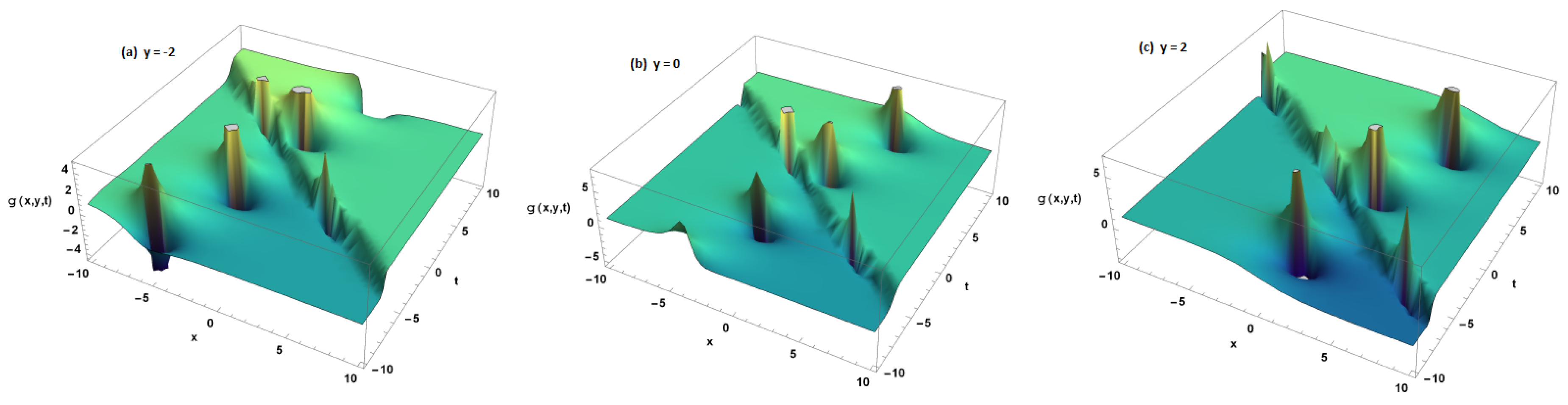
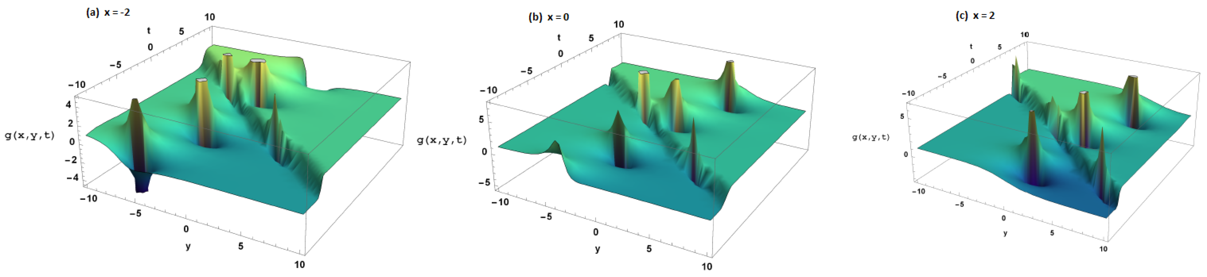
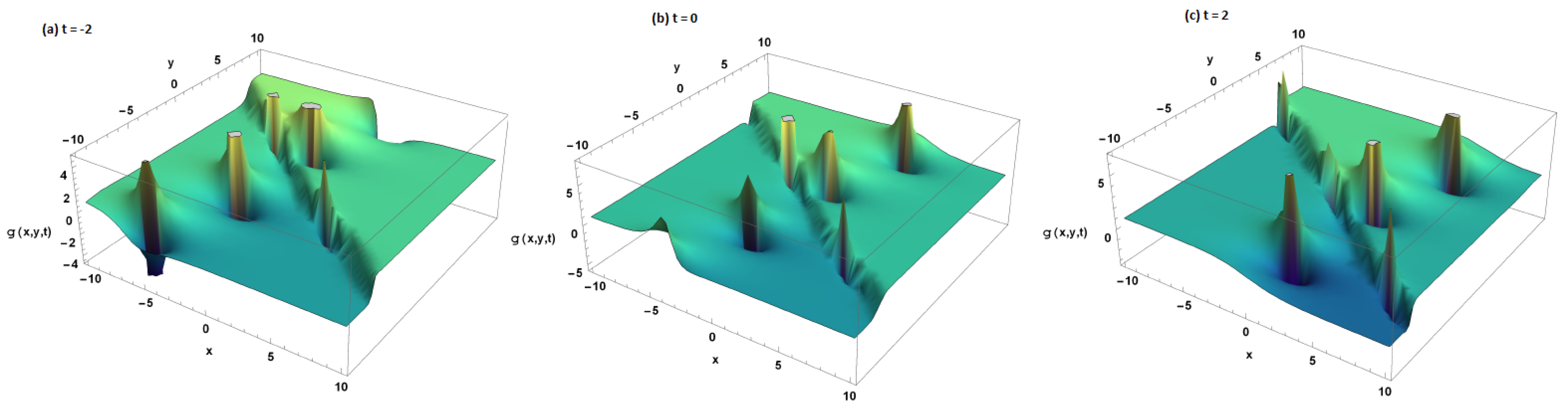
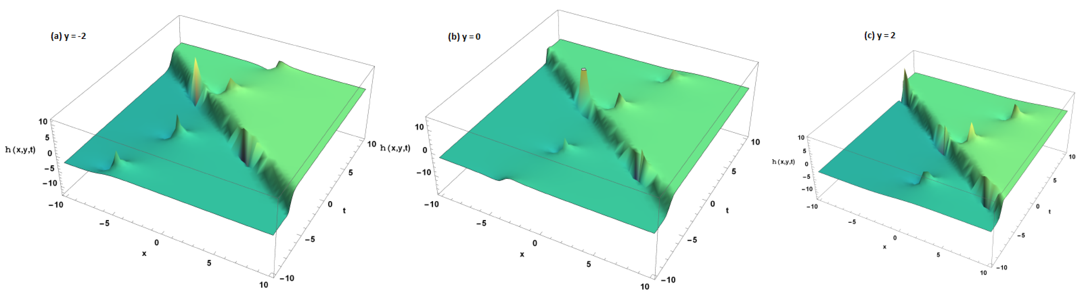
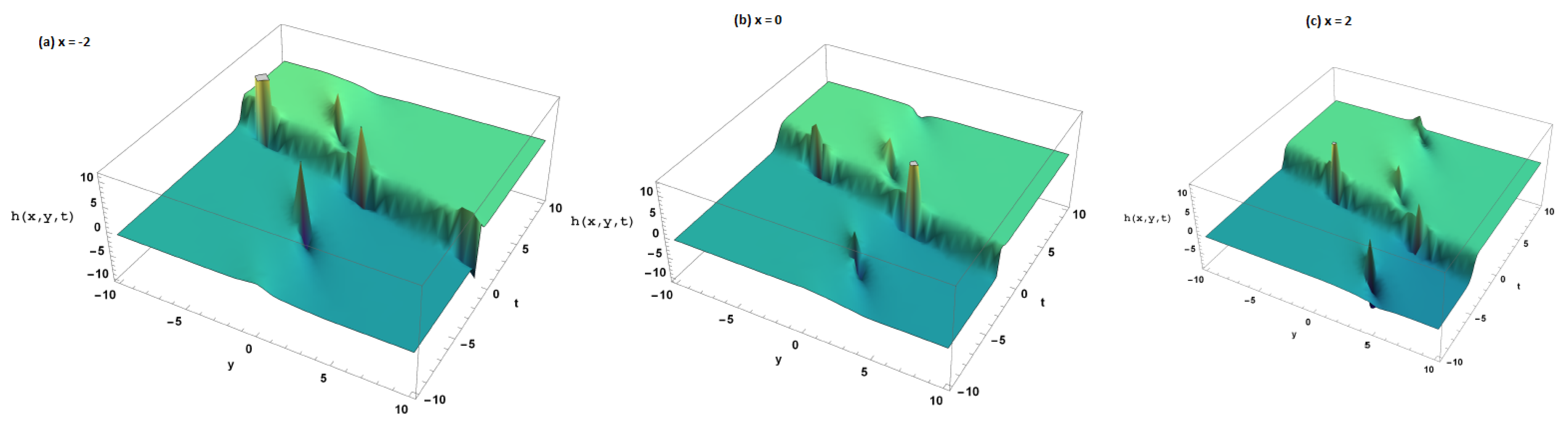
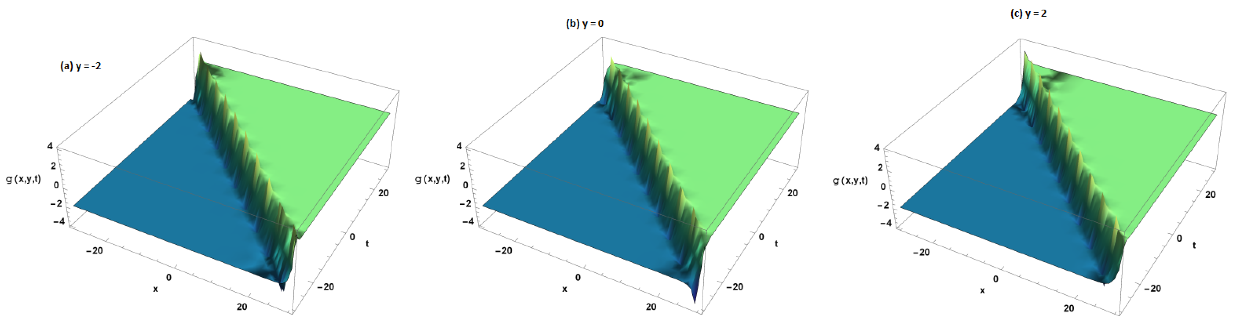
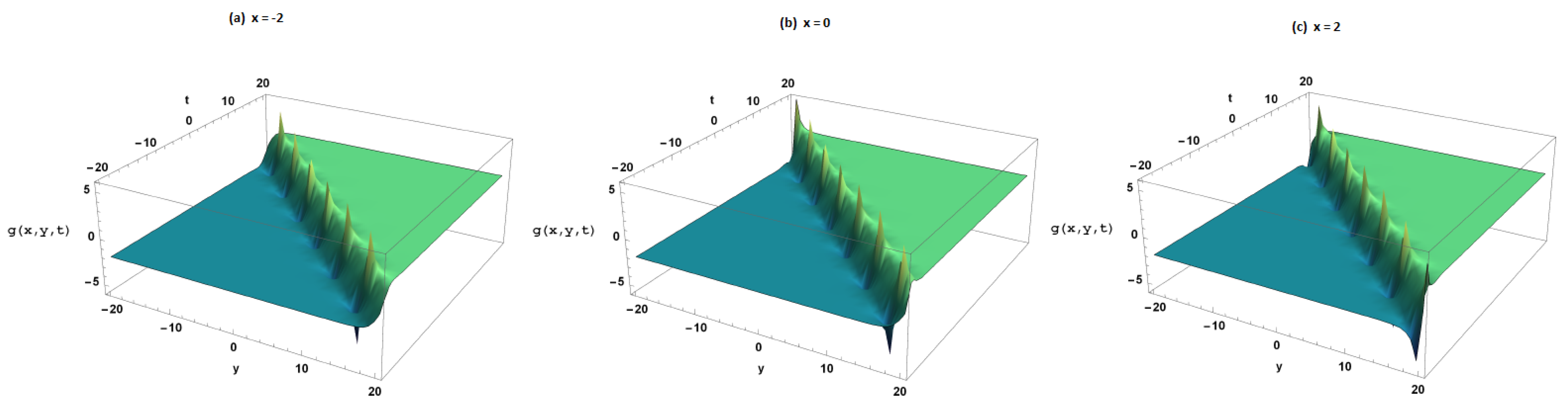
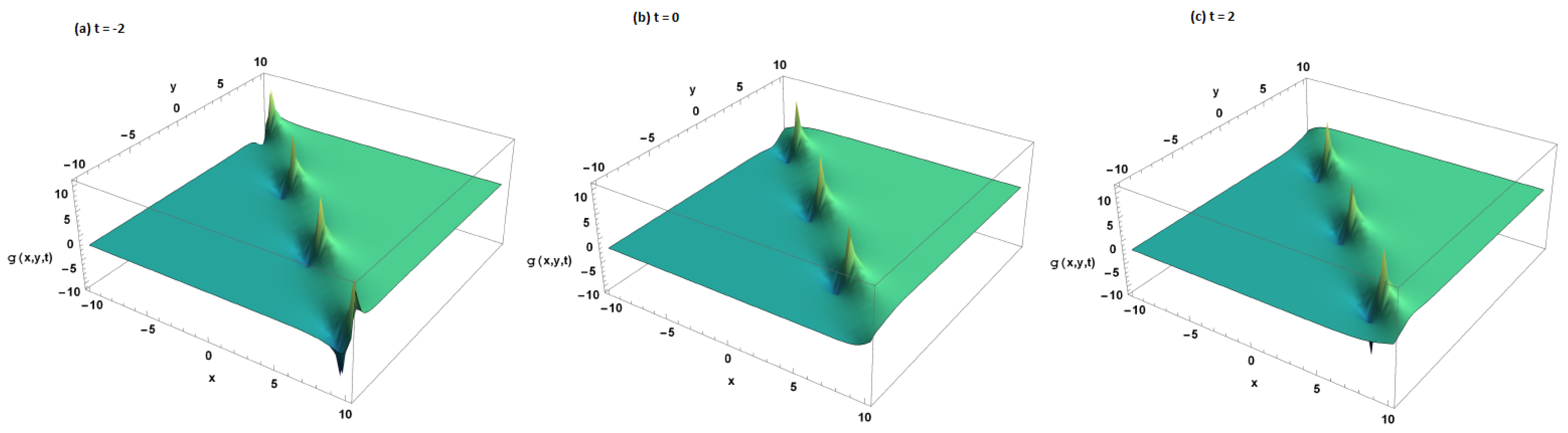
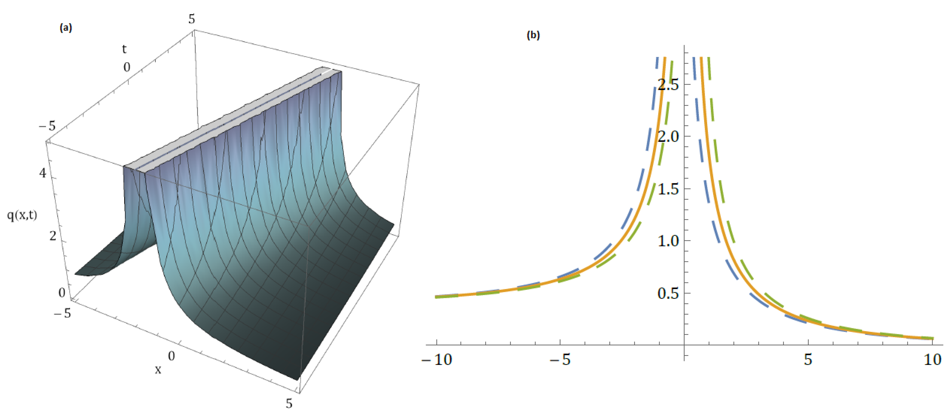
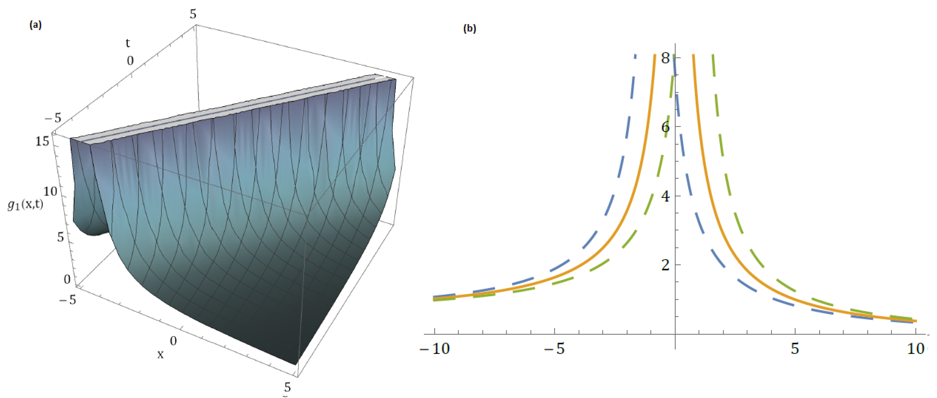
4. Graphical Representation of Solutions

In this section, some suitable numerical values of parameters selected for our analytical three wave solitons and periodic wave solutions are represented in the following Figures. In Figure 1, we gave graphs for new three wave solution (20), with suitable values of parameters, (a) in $y=-2$, (b) in $y=0$ and (c) in $y=2$ with $a=1,a_1=1,a_2=1,{\kappa }_3=-2,{\kappa }_1=1,b_1=1,b_2=1,b_3=1,$$g_0=1,h_0=1,{\kappa }_2=1,b=1$ $-10<t<10$ and $-10<x<10$. In Figure 2, we gave graphs for new three wave solution (20), with suitable values of parameters, (a) in $x=-2$, (b) in $x=0$ and (c) in $x=2$ with $a=1,a_1=1,a_2=1,{\kappa }_3=-2,{\kappa }_1=1,b_1=1,b_2=1,b_3=1,g_0=1,h_0=1,{\kappa }_2=1,b=1$ $-10<t<10$ and $-10<Y<10$. In Figure 3, we gave graphs for new three wave solution (20), with suitable values of parameters, (a) in $t=-2$, (b) in $t=0$ and (c) in $t=2$ with $a=1,a_1=1,a_2=1,$${\kappa }_3=-2,{\kappa }_1=1,b_1=1,b_2=1,b_3=1,g_0=1,h_0=1,{\kappa }_2=1,b=1$ $-10<x<10$ and $-10<y<10$. In Figure 4, we gave graphs for new three wave solution (21), with suitable values of parameters, (a) in $y=-2$, (b) in $y=0$ and (c) in $y=2$ with $a=1,a_1=1,a_2=1,$${\kappa }_3=-2,{\kappa }_1=1,b_1=1,b_2=1,b_3=1,g_0=1,h_0=1,{\kappa }_2=1,b=1$ $-10<t<10$ and $-10<x<10$. In Figure 5, we gave graphs for new three wave solution (21), with suitable values of parameters, (a) in $x=-2$, (b) in $x=0$ and (c) in $x=2$ with $a=1,a_1=1,a_2=1,$${\kappa }_3=-2,{\kappa }_1=1,b_1=1,b_2=1,b_3=1,g_0=1,h_0=1,{\kappa }_2=1,b=1$ $-10<t<10$ and $-10<Y<10$. In Figure 6, we gave graphs for new three wave solution (21), with suitable values of parameters, (a) in $t=-2$, (b) in $t=0$ and (c) in $t=2$ with $a=1,a_1=1,a_2=1,{\kappa }_3=-2,$${\kappa }_1=1,b_1=1,b_2=1,b_3=1,g_0=1,h_0=1,{\kappa }_2=1,b=1$ $-10<x<10$ and $-10<y<10$. In Figure 7, we gave graphs for new periodic solution (33), with suitable values of parameters, (a) in $y=-2$, (b) in $y=0$ and (c) in $y=2$ with $a=1,a_1=1,a_2=1,{\kappa }_3=-2,{\kappa }_1=1,b_1=1,b_2=1,$$b_3=1,g_0=1,h_0=1,{\kappa }_2=1,b=1,{\kappa }_4=1,c_4=2,a_4=2,c_2=1,p=1$ $-30<t<30$ and $-30<x<30$. In Figure 8, we gave graphs for new periodic solution (33), with suitable values of parameters, (a) in $x=-2$, (b) in $x=0$ and (c) in $x=2$ with $a=1,a_1=1,a_2=1,{\kappa }_3=-2,$${\kappa }_1=1,b_1=1,b_2=1,b_3=1,g_0=1,h_0=1,{\kappa }_2=1,b=1,{\kappa }_4=1,c_4=2,a_4=2,c_2=1,p=1$ $-20<t<20$ and $-20<Y<20$. In Figure 9, we gave graphs for new periodic solution (33), with suitable values of parameters, (a) in $t=-2$, (b) in $t=0$ and (c) in $t=2$ with $a=1,a_1=1,a_2=1,$${\kappa }_3=-2,{\kappa }_1=1,b_1=1,b_2=1,b_3=1,g_0=1,h_0=1,{\kappa }_2=1,b=1,{\kappa }_4=1,c_4=2,a_4=2,$$c_2=1,p=1$ $-10<x<10$ and $-10<y<10$. In Figure 10, we gave graphs for solution (84), with suitable values of parameters, a 3D graph shown in (a) with $\mathsf{\Omega }=1,b=1,\tau =0.1,a=0.5,y=0$ $-5<x<5$ and $-5<t<5$ and a 2D graph shown in (b) with $\mathsf{\Omega }=1,b=1,\tau =0.1,a=0.5,y=0$ $-10<x<10$ and $-1<t<1$. In Figure 11, we gave graphs for solution (95), with suitable values of parameters, a 3D graph shown in (a) with $\mathsf{\Omega }=2.3,b=1.4,\tau =0.1,a=0.5,y=0$ $-5<x<5$ and $-5<t<5$ and a 2D graph shown in (b) with $\mathsf{\Omega }=2.3,b=1.4,\tau =0.1,a=0.5,y=0$ $-10<x<10$ and $-1<t<1$.

5. Conclusions

In this paper, we succeed to obtain the new three wave, periodic wave and other exact wave solutions to the (2+1)-dimensional Burgers equations by utilizing the Hirota bilinear and EShGEE schemes. Achieved solutions are verified and demonstrated by different plots with the use of Mathematica software. Some of the achieved solutions are also described graphically by two-dimensional, three-dimensional and contour plots. Our research model Burgers equation is a fundamental partial differential equation from fluid mechanics. It occurs in many fields of applied mathematics such as modeling of gas dynamics, traffic flow, etc. The schemes that are used in this research have never been applied to this model before, and the obtained results are newer than the existing results of this model in the literature. The diverse graphical analyses for the presented solutions show that the solutions are reliable for the further development in the model, and also in other areas of mathematical physics and engineering; for example, in communication, optical computing, optical switching, etc. Finally, these two schemes are simple, fruitful and reliable to handle the nonlinear PDEs.

References

1. Sandeep, M.; Kumar, S.; Biswas, A.; Yıldırım, Y.; Moraru, L.; Moldovanu, S.; Iticescu, C.; Alotaibi, A. Highly dispersive optical solitons in the absence of self-phase modulation by lie symmetry. Symmetry 2023, 15, 886. [Google Scholar]
2. Sachin, K.; Biswas, A.; Yıldırım, Y.; Moraru, L.; Moldovanu, S.; Alshehri, H.M.; Maturi, D.A.; Al-Bogami, D.H. Cubic–quartic optical soliton perturbation with differential group delay for the Lakshmanan–Porsezian–Daniel model by Lie symmetry. Symmetry 2022, 14, 224. [Google Scholar]
3. Asghari, Y.; Eslami, M.; Rezazadeh, H. Exact solutions to the conformable time-fractional discretized mKdv lattice system using the fractional transformation method. Opt. Quantum Electron. 2023, 55, 318. [Google Scholar] [CrossRef]
4. Kudryashov, N.A. Method for finding highly dispersive optical solitons of nonlinear differential equations. Optik 2020, 206, 163550. [Google Scholar] [CrossRef]
5. Iqbal, M.A.; Wang, Y.; Miah, M.M.; Osman, M.S. Study on date–Jimbo–Kashiwara–Miwa equation with conformable derivative dependent on time parameter to find the exact dynamic wave solutions. Fractal Fract. 2021, 6, 4. [Google Scholar] [CrossRef]
6. Wu, G.; Guo, Y. New Complex Wave Solutions and Diverse Wave Structures of the (2+1)-Dimensional Asymmetric Nizhnik–Novikov–Veselov Equation. Fractal Fract. 2023, 7, 170. [Google Scholar] [CrossRef]
7. Almusawa, H.; Jhangeer, A. A study of the soliton solutions with an intrinsic fractional discrete nonlinear electrical transmission line. Fractal Fract. 2022, 6, 334. [Google Scholar] [CrossRef]
8. Areshi, M.; Seadawy, A.R.; Ali, A.; Alharbi, A.F.; Aljohani, A.F. Analytical Solutions of the Predator–Prey Model with Fractional Derivative Order via Applications of Three Modified Mathematical Methods. Fractal Fract. 2023, 7, 128. [Google Scholar] [CrossRef]
9. Abdelwahed, H.G.; Alsarhana, A.F.; El-Shewy, E.K.; Abdelrahman, M.A.E. The Stochastic Structural Modulations in Collapsing Maccari’s Model Solitons. Fractal Fract. 2023, 7, 290. [Google Scholar] [CrossRef]
10. Zafar, A.; Raheel, M.; Rezazadeh, H.; Inc, M.; Akinlar, M.A. New chirp-free and chirped form optical solitons to the non-linear Schrödinger equation. Opt. Quantum Electron. 2021, 53, 604. [Google Scholar] [CrossRef]
11. Rahman, Z.; Abdeljabbar, A.; Ali, M.Z. Novel precise solitary wave solutions of two time fractional nonlinear evolution models via the MSE scheme. Fractal Fract. 2022, 6, 444. [Google Scholar] [CrossRef]
12. Shqair, M.; Alabedalhadi, M.; Al-Omari, S.; Al-Smadi, M. Abundant exact travelling wave solutions for a fractional massive Thirring model using extended Jacobi elliptic function method. Fractal Fract. 2022, 6, 252. [Google Scholar] [CrossRef]
13. Mohammed, W.W.; Al-Askar, F.M.; Cesarano, C.; El-Morshedy, M. On the Dynamics of Solitary Waves to a (3+1)-Dimensional Stochastic Boiti–Leon–Manna–Pempinelli Model in Incompressible Fluid. Mathematics 2023, 11, 2390. [Google Scholar] [CrossRef]
14. Mohammed, W.W.; Cesarano, C. The soliton solutions for the (4+1)-dimensional stochastic Fokas equation. Math. Methods Appl. Sci. 2023, 46, 7589–7597. [Google Scholar] [CrossRef]
15. Mohammed, W.W.; Albosaily, S.; Iqbal, N.; El-Morshedy, M. The effect of multiplicative noise on the exact solutions of the stochastic Burgers’ equation. Waves Random Complex Media 2021, 1–13. [Google Scholar] [CrossRef]
16. Liu, J.; Du, J.; Zeng, Z.; Nie, B. New three-wave solutions for the (3+1)-dimensional Boiti–Leon–Manna–Pempinelli equation. Nonlinear Dyn. 2017, 88, 655–661. [Google Scholar] [CrossRef]
17. Ilhan, O.A.; Manafian, J. Periodic type and periodic cross-kink wave solutions to the (2+1)-dimensional breaking soliton equation arising in fluid dynamics. Mod. Phys. Lett. B 2019, 33, 1950277. [Google Scholar] [CrossRef]
18. Ali, K.K.; Raheel, M.; Inc, M. Some new types of optical solitons to the time-fractional new hamiltonian amplitude equation via extended Sinh-Gorden equation expansion method. Mod. Phys. Lett. B 2022, 36, 2250089. [Google Scholar] [CrossRef]
19. Zafar, A.; Bekir, A.; Raheel, M.; Razzaq, W. Optical soliton solutions to Biswas–Arshed model with truncated M-fractional derivative. Optik 2020, 222, 165355. [Google Scholar] [CrossRef]
20. Wang, Q.; Chen, Y.; Zhang, H.Q. A new Riccati equation rational expansion method and its application to (2+1)-dimensional Burgers equation. Chaos Solitons Fractals 2005, 25, 1019–1028. [Google Scholar] [CrossRef]
21. Wang, H. Lump and interaction solutions to the (2+1)-dimensional Burgers equation. Appl. Math. Lett. 2018, 85, 27–34. [Google Scholar] [CrossRef]
22. Wang, D.-S.; Li, H.-B.; Wang, J. The novel solutions of auxiliary equation and their application to the (2+1)-dimensional Burgers equations. Chaos Solitons Fractals 2008, 38, 374–382. [Google Scholar] [CrossRef]
23. Li, Z.; Manafian, J.; Ibrahimov, N.; Hajar, A.; Nisar, K.S.; Jamshed, W. Variety interaction between k-lump and k-kink solutions for the generalized Burger equation with variable coefficients by bilinear analysis. Results Phys. 2021, 28, 104490. [Google Scholar] [CrossRef]
24. Yang, X.L.; Tang, J.S. Travelling wave solutions for Konopelchenko-Dubrovsky equation using an extended sinh-Gordon equation expansion method. Commun. Theor. Phys. 2008, 50, 10471051. [Google Scholar]
Figure 1. In this graph shows three wave behavior with different fix values of y in (a) y = 2 , in (b) y = 0 and in (c) y = 2 contour surfaces representation of (20).
Symmetry 15 01573 g001
Figure 2. In this graph shows three wave behavior with different fix values of x in (a) x = 2 , in (b) x = 0 and in (c) x = 2 contour surfaces representation of (20).
Symmetry 15 01573 g002
Figure 3. In this graph shows three wave behavior with different fix values of t in (a) t = 2 , in (b) t = 0 and in (c) t = 2 contour surfaces representation of (20).
Symmetry 15 01573 g003
Figure 4. In this graph shows three wave behavior with different fix values of y in (a) y = 2 , in (b) y = 0 and in (c) y = 2 contour surfaces representation of (21).
Symmetry 15 01573 g004
Figure 5. In this graph shows three wave behavior with different fix values of x in (a) x = 2 , in (b) x = 0 and in (c) x = 2 contour surfaces representation of (21).
Symmetry 15 01573 g005
Figure 6. In this graph shows three wave behavior with different fix values of t in (a) t = 2 , in (b) t = 0 and in (c) t = 2 contour surfaces representation of (21).
Symmetry 15 01573 g006
Figure 7. In this graph shows periodic wave behavior with different fix values of y in (a) y = 2 , in (b) y = 0 and in (c) y = 2 contour surfaces representation of (33).
Symmetry 15 01573 g007
Figure 8. In this graph shows periodic wave behavior with different fix values of x in (a) x = 2 , in (b) x = 0 and in (c) x = 2 contour surfaces representation of (33).
Symmetry 15 01573 g008
Figure 9. In this graph shows periodic wave behavior with different fix values of t in (a) t = 2 , in (b) t = 0 and in (c) t = 2 contour surfaces representation of (33).
Symmetry 15 01573 g009
Figure 10. In this graph shows wave behavior 3D in (a) and 2D in (b) surfaces representation of (84).
Symmetry 15 01573 g010
Figure 11. In this figure graph shows wave behavior 3D in (a) and 2D in (b) surfaces representation of (95).
Symmetry 15 01573 g011
Disclaimer/Publisher’s Note: The statements, opinions and data contained in all publications are solely those of the individual author(s) and contributor(s) and not of MDPI and/or the editor(s). MDPI and/or the editor(s) disclaim responsibility for any injury to people or property resulting from any ideas, methods, instructions or products referred to in the content.