Author Contributions
Conceptualization, O.H.O., H.M.A. and Z.A.; methodology, O.H.O., H.M.A. and Z.A.; software, O.H.O., Z.A., F.K. and A.A.-A.H.E.-B.; validation, O.H.O. and Z.A.; formal analysis, H.M.A., O.H.O., Z.A. and F.K.; investigation, O.H.O. and A.A.-A.H.E.-B.; data curation, Z.A. and F.K.; writing—original draft preparation, O.H.O., H.M.A., Z.A., F.K. and A.A.-A.H.E.-B.; writing—review and editing, O.H.O., H.M.A. and Z.A.; visualization, H.M.A., Z.A., F.K. and A.A.-A.H.E.-B. All authors have read and agreed to the published version of the manuscript.
Figure 1.
For different values of and , the visual illustrations of (a) and (b) of the NCT-Weibull distribution.
Figure 1.
For different values of and , the visual illustrations of (a) and (b) of the NCT-Weibull distribution.
Figure 2.
Different plots of of the NCT-Weibull distribution, including (a) right-skewed, (b) decreasing, (c) symmetrical, and (d) left-skewed.
Figure 2.
Different plots of of the NCT-Weibull distribution, including (a) right-skewed, (b) decreasing, (c) symmetrical, and (d) left-skewed.
Figure 3.
Different plots of of the NCT-Weibull distribution, including (a) increasing, (b) decreasing, (c) bathtub, and (d) modified unimodal.
Figure 3.
Different plots of of the NCT-Weibull distribution, including (a) increasing, (b) decreasing, (c) bathtub, and (d) modified unimodal.
Figure 4.
A graphical illustration of the coefficients of skewness and kurtosis of the NCT-Weibull distribution.
Figure 4.
A graphical illustration of the coefficients of skewness and kurtosis of the NCT-Weibull distribution.
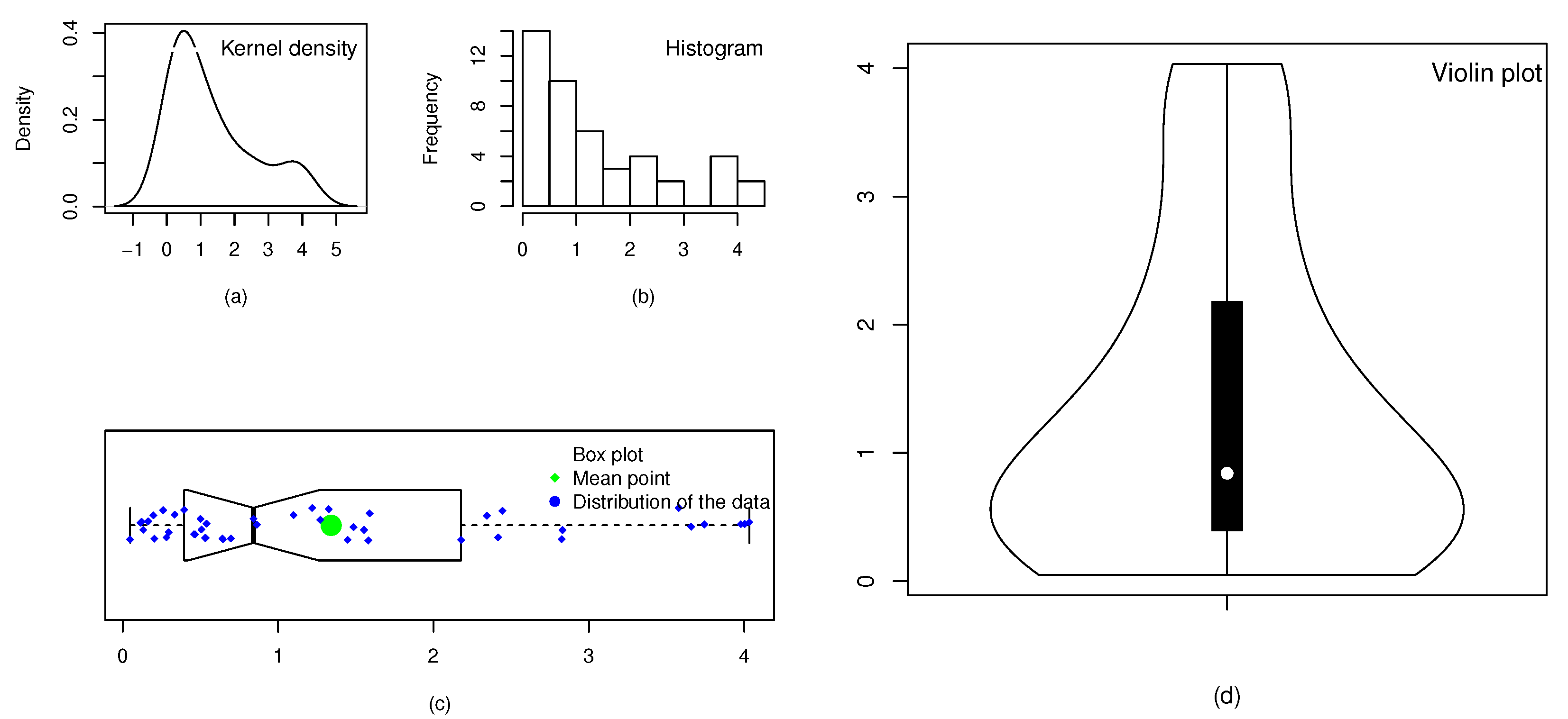
Figure 5.
The chemotherapy dataset represented by (a) kernel density plot, (b) histogram, (c) box plot, and (d) violin plot.
Figure 5.
The chemotherapy dataset represented by (a) kernel density plot, (b) histogram, (c) box plot, and (d) violin plot.
Figure 6.
The acute myelogenous leukemia dataset represented by (a) kernel density plot, (b) histogram, (c) box plot, and (d) violin plot.
Figure 6.
The acute myelogenous leukemia dataset represented by (a) kernel density plot, (b) histogram, (c) box plot, and (d) violin plot.
Figure 7.
The profiles of the LLF of (a) and (b) of the NCT-Weibull distribution for the chemotherapy treatment dataset.
Figure 7.
The profiles of the LLF of (a) and (b) of the NCT-Weibull distribution for the chemotherapy treatment dataset.
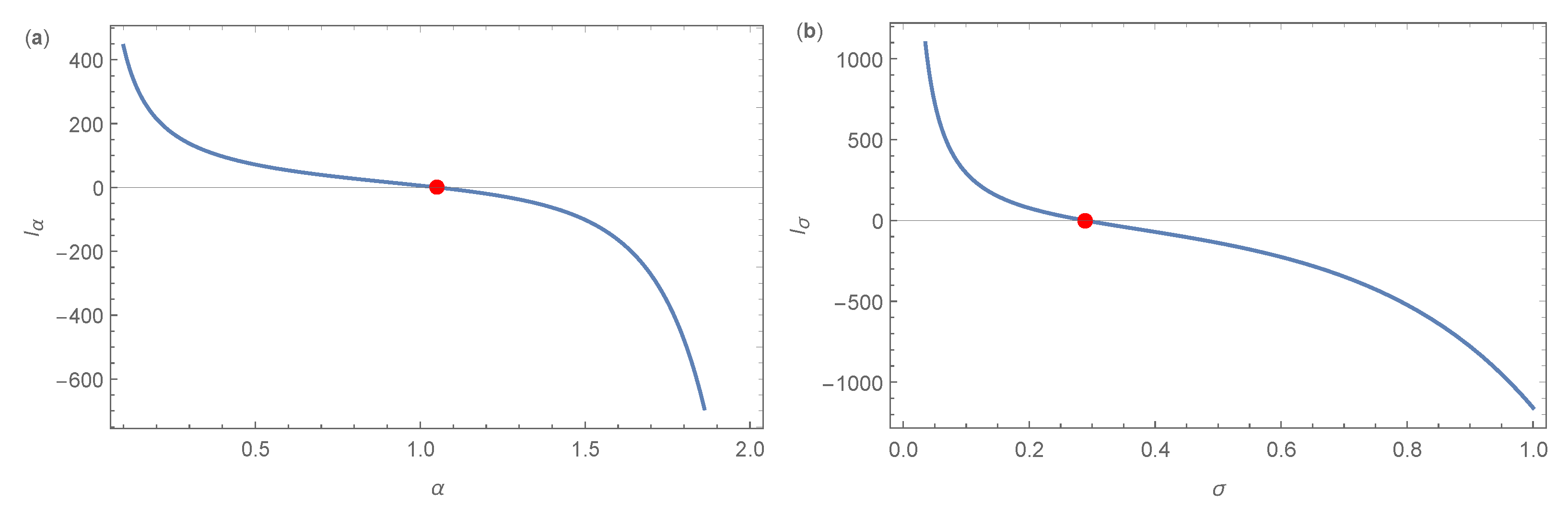
Figure 8.
The visual illustrations of the existence of (a) and (b) of the NCT-Weibull distribution for the chemotherapy treatment dataset.
Figure 8.
The visual illustrations of the existence of (a) and (b) of the NCT-Weibull distribution for the chemotherapy treatment dataset.
Figure 9.
The fitted PDF plots of the (a) NCT-Weibull, (b) Weibull, (c) NEE-Weibull, and (d) NAC-Weibull for the chemotherapy treatment dataset.
Figure 9.
The fitted PDF plots of the (a) NCT-Weibull, (b) Weibull, (c) NEE-Weibull, and (d) NAC-Weibull for the chemotherapy treatment dataset.
Figure 10.
Corresponding to the chemotherapy treatment dataset, the fitted (a) CDF and (b) SF of the NCT-Weibull distribution and rival models.
Figure 10.
Corresponding to the chemotherapy treatment dataset, the fitted (a) CDF and (b) SF of the NCT-Weibull distribution and rival models.
Figure 11.
The profiles of the LLF of (a) and (b) of the NCT-Weibull distribution for the acute myelogenous leukemia dataset.
Figure 11.
The profiles of the LLF of (a) and (b) of the NCT-Weibull distribution for the acute myelogenous leukemia dataset.
Figure 12.
The visual illustrations of the existence of (a) and (b) of the NCT-Weibull distribution for the acute myelogenous leukemia dataset.
Figure 12.
The visual illustrations of the existence of (a) and (b) of the NCT-Weibull distribution for the acute myelogenous leukemia dataset.
Figure 13.
The fitted PDF plots of the (a) NCT-Weibull, (b) Weibull, (c) NEE-Weibull, and (d) NAC-Weibull for the acute myelogenous leukemia dataset.
Figure 13.
The fitted PDF plots of the (a) NCT-Weibull, (b) Weibull, (c) NEE-Weibull, and (d) NAC-Weibull for the acute myelogenous leukemia dataset.
Figure 14.
Corresponding to the acute myelogenous leukemia dataset, the fitted (a) CDF and (b) SF of the NCT-Weibull distribution and rival models.
Figure 14.
Corresponding to the acute myelogenous leukemia dataset, the fitted (a) CDF and (b) SF of the NCT-Weibull distribution and rival models.
Table 1.
Numerical values for quartiles along with coefficients of skewnenss and kurtosis of the NCT-Weibull distribution.
Table 1.
Numerical values for quartiles along with coefficients of skewnenss and kurtosis of the NCT-Weibull distribution.
| Parameters | Measures |
|---|
| | | | | | |
| 0.25 | 0.25 | 0.0450 | 1.6655 | 27.2954 | 0.8811 | 4.4220 |
| 0.7 | 0.3304 | 1.1998 | 3.2575 | 0.4059 | 1.4424 |
| 1.0 | 0.4606 | 1.1360 | 2.2857 | 0.2599 | 1.2547 |
| 1.5 | 0.5964 | 1.0887 | 1.7353 | 0.1354 | 1.1798 |
| 2.5 | 0.7334 | 1.0522 | 1.3918 | 0.0316 | 1.1715 |
| 4.0 | 0.8239 | 1.0324 | 1.2296 | −0.0278 | 1.1887 |
| 0.7 | 0.25 | 0.0007 | 0.0272 | 0.4441 | 0.8806 | 4.4202 |
| 0.7 | 0.0759 | 0.2756 | 0.7484 | 0.4060 | 1.4422 |
| 1.0 | 0.1645 | 0.4057 | 0.8163 | 0.2598 | 1.2552 |
| 1.5 | 0.3002 | 0.5480 | 0.8733 | 0.1352 | 1.1803 |
| 2.5 | 0.4858 | 0.6972 | 0.9221 | 0.0307 | 1.1718 |
| 4.0 | 0.6368 | 0.7981 | 0.9505 | −0.0282 | 1.1883 |
| 1.0 | 0.25 | 0.0001 | 0.0065 | 0.1066 | 0.8810 | 4.42203 |
| 0.7 | 0.0457 | 0.1654 | 0.4496 | 0.4071 | 1.4428 |
| 1.0 | 0.1152 | 0.2840 | 0.5715 | 0.2600 | 1.2545 |
| 1.5 | 0.2367 | 0.4321 | 0.6886 | 0.1353 | 1.1802 |
| 2.5 | 0.4212 | 0.6045 | 0.7994 | 0.0309 | 1.1711 |
| 4.0 | 0.5825 | 0.7300 | 0.8695 | −0.0280 | 1.1888 |
| 1.5 | 0.25 | 0.5825 | 0.7300 | 0.8695 | −0.0280 | 1.1888 |
| 0.7 | 0.0254 | 0.0928 | 0.2519 | 0.4046 | 1.4421 |
| 1.0 | 0.0767 | 0.1894 | 0.3808 | 0.2592 | 1.2551 |
| 1.5 | 0.1807 | 0.3297 | 0.5255 | 0.1355 | 1.1800 |
| 2.5 | 0.3581 | 0.5140 | 0.6799 | 0.0313 | 1.1705 |
| 4.0 | 0.5263 | 0.6596 | 0.7856 | −0.0284 | 1.1890 |
| 2.5 | 0.25 | 4 × | 0.0005 | 0.0028 | 0.6667 | 4.4566 |
| 0.7 | 0.0123 | 0.0447 | 0.1214 | 0.4059 | 1.4439 |
| 1.0 | 0.0460 | 0.1136 | 0.2285 | 0.2590 | 1.2562 |
| 1.5 | 0.1285 | 0.2346 | 0.3738 | 0.1353 | 1.1803 |
| 2.5 | 0.2921 | 0.4189 | 0.5541 | 0.0318 | 1.1721 |
| 4.0 | 0.4634 | 0.5806 | 0.6914 | −0.0278 | 1.1899 |
| 4.0 | 0.25 | 6 × | 0.0005 | 0.0007 | −0.3333 | 2.1218 |
| 0.7 | 0.0064 | 0.0230 | 0.0620 | 0.4017 | 1.4498 |
| 1.0 | 0.0290 | 0.0711 | 0.1430 | 0.2603 | 1.2565 |
| 1.5 | 0.0939 | 0.1713 | 0.2734 | 0.1377 | 1.1792 |
| 2.5 | 0.2419 | 0.3470 | 0.4592 | 0.0324 | 1.1705 |
| 4.0 | 0.4119 | 0.5162 | 0.6149 | −0.0277 | 1.1879 |
Table 2.
The numerical description of the SS of the NCT-Weibull distribution for and .
Table 2.
The numerical description of the SS of the NCT-Weibull distribution for and .
| n | Parameters | MLE | MSE | Bias |
|---|
| | | 0.9355044 | 0.01082877 | 0.035504420 |
| 50 | | 1.5807460 | 0.06715720 | 0.080745775 |
| | | 0.9201044 | 0.00479964 | 0.020104365 |
| 100 | | 1.5444920 | 0.03049332 | 0.044492288 |
| | | 0.9151175 | 0.00277550 | 0.015117474 |
| 200 | | 1.5243870 | 0.01430133 | 0.024387130 |
| | | 0.9105759 | 0.00186720 | 0.010575924 |
| 300 | | 1.5193200 | 0.00989402 | 0.019319599 |
| | | 0.9084876 | 0.00125306 | 0.008487576 |
| 400 | | 1.5145360 | 0.00661767 | 0.014535798 |
| | | 0.9073618 | 0.00094190 | 0.007361801 |
| 500 | | 1.5099910 | 0.00507208 | 0.009991227 |
| | | 0.9048286 | 0.00076818 | 0.004828569 |
| 1000 | | 1.5098150 | 0.00412407 | 0.009415482 |
| | | 0.9046138 | 0.00062513 | 0.004613809 |
| 1500 | | 1.5079170 | 0.00356039 | 0.008917051 |
| | | 0.9045965 | 0.00058086 | 0.004596521 |
| 2000 | | 1.504196 | 0.00286160 | 0.004196165 |
| | | 0.9040372 | 0.00043847 | 0.004507215 |
| 2500 | | 1.5038410 | 0.00201378 | 0.003840787 |
| | | 0.9030904 | 0.00037242 | 0.004190369 |
| 3000 | | 1.5027150 | 0.00215174 | 0.003315493 |
| | | 0.9022970 | 0.00035733 | 0.004096963 |
| 3500 | | 1.5018020 | 0.00162623 | 0.002802116 |
| | | 0.9014026 | 0.00022969 | 0.003402595 |
| 4000 | | 1.5011270 | 0.00132665 | 0.002427410 |
| | | 0.9010336 | 0.00022699 | 0.002733606 |
| 4500 | | 1.5003060 | 0.00110904 | 0.002005540 |
| | | 0.9002476 | 0.00020651 | 0.001147633 |
| 5000 | | 1.5001260 | 0.00108060 | 0.004276054 |
Table 3.
The numerical description of the SS of the NCT-Weibull distribution for and .
Table 3.
The numerical description of the SS of the NCT-Weibull distribution for and .
| n | Parameters | MLE | MSE | Bias |
|---|
| | | 1.647293 | 0.03745800 | 0.04729255 |
| 50 | | 1.257434 | 0.04245403 | 0.05743403 |
| | | 1.627257 | 0.01732586 | 0.02725739 |
| 100 | | 1.235155 | 0.01727730 | 0.03515506 |
| | | 1.618928 | 0.00993020 | 0.01892835 |
| 200 | | 1.216921 | 0.00978696 | 0.01692071 |
| | | 1.610806 | 0.00749452 | 0.01080646 |
| 300 | | 1.209155 | 0.00590437 | 0.00915519 |
| | | 1.607756 | 0.00578927 | 0.00875570 |
| 400 | | 1.207724 | 0.00522039 | 0.00772403 |
| | | 1.607377 | 0.00495649 | 0.00837722 |
| 500 | | 1.206386 | 0.00413462 | 0.00638614 |
| | | 1.607077 | 0.00404159 | 0.00807700 |
| 1000 | | 1.204783 | 0.00370541 | 0.00608253 |
| | | 1.605926 | 0.00357296 | 0.00592560 |
| 1500 | | 1.202933 | 0.00310211 | 0.00553341 |
| | | 1.605566 | 0.00342711 | 0.00506591 |
| 2000 | | 1.201824 | 0.00299849 | 0.00524317 |
| | | 1.603931 | 0.00269719 | 0.00430580 |
| 2500 | | 1.201376 | 0.00258171 | 0.00437642 |
| | | 1.603272 | 0.00248891 | 0.00427248 |
| 3000 | | 1.201039 | 0.00238806 | 0.00383875 |
| | | 1.602213 | 0.00226258 | 0.00381321 |
| 3500 | | 1.200925 | 0.00215743 | 0.00332455 |
| | | 1.601890 | 0.00211945 | 0.00338986 |
| 4000 | | 1.200769 | 0.00206960 | 0.00286931 |
| | | 1.600817 | 0.00197970 | 0.00301707 |
| 4500 | | 1.200167 | 0.00170270 | 0.00216691 |
| | | 1.600798 | 0.00118820 | 0.00149835 |
| 5000 | | 1.200115 | 0.00124240 | 0.00139478 |
Table 4.
The numerical description of the SS of the NCT-Weibull distribution for and .
Table 4.
The numerical description of the SS of the NCT-Weibull distribution for and .
| n | Parameters | MLE | MSE | Bias |
|---|
| | | 1.536557 | 0.02935531 | 0.036556898 |
| 50 | | 1.032626 | 0.02028196 | 0.032626058 |
| | | 1.523453 | 0.01454322 | 0.023453154 |
| 100 | | 1.022780 | 0.01560843 | 0.022780097 |
| | | 1.512594 | 0.00878291 | 0.018594240 |
| 200 | | 1.012194 | 0.00617592 | 0.012193633 |
| | | 1.512682 | 0.00751053 | 0.012682101 |
| 300 | | 1.011429 | 0.00479729 | 0.011428825 |
| | | 1.509734 | 0.00474624 | 0.009734084 |
| 400 | | 1.008920 | 0.00435279 | 0.008920038 |
| | | 1.506511 | 0.00435750 | 0.007510780 |
| 500 | | 1.008418 | 0.00389977 | 0.007417519 |
| | | 1.505726 | 0.00376879 | 0.006726321 |
| 1000 | | 1.007672 | 0.00348127 | 0.007071814 |
| | | 1.505137 | 0.00321440 | 0.005837298 |
| 1500 | | 1.006518 | 0.00312391 | 0.005518071 |
| | | 1.503928 | 0.00292193 | 0.005128123 |
| 2000 | | 1.005165 | 0.00296230 | 0.004164561 |
| | | 1.502614 | 0.00273244 | 0.004613729 |
| 2500 | | 1.004497 | 0.00250790 | 0.003497397 |
| | | 1.501920 | 0.00244730 | 0.003920174 |
| 3000 | | 1.003782 | 0.00201760 | 0.002781555 |
| | | 1.501252 | 0.00220965 | 0.002252233 |
| 3500 | | 1.002927 | 0.00143502 | 0.002427178 |
| | | 1.501022 | 0.00181327 | 0.001721648 |
| 4000 | | 1.002255 | 0.00130605 | 0.002254885 |
| | | 1.500701 | 0.00144591 | 0.001300919 |
| 4500 | | 1.002055 | 0.00118396 | 0.002055212 |
| | | 1.500362 | 0.00106532 | 0.000932209 |
| 5000 | | 1.004314 | 0.00113503 | 0.001313930 |
Table 5.
Key measures of the chemotherapy and acute myelogenous leukemia data.
Table 5.
Key measures of the chemotherapy and acute myelogenous leukemia data.
| Description | Mean | 1st Quartile | 2nd Quartile | 3rd Quartile |
|---|
| Data 1 | 1.341 | 0.395 | 0.841 | 2.178 |
| Data 2 | 42.060 | 4.000 | 22.000 | 65.000 |
| Description | Standard deviation | Variance | Minimum | Maximum |
| Data 1 | 1.246 | 1.554 | 0.047 | 4.033 |
| Data 2 | 46.944 | 2203.802 | 1.00 | 156.00 |
| Description | Range | Skewness | Kurtosis | Data size |
| Data 1 | 3.986 | 0.972 | 2.663 | 45 |
| Data 2 | 155 | 1.124 | 3.026 | 32 |
Table 6.
The numerical values of and of the fitted models for the chemotherapy treatment dataset.
Table 6.
The numerical values of and of the fitted models for the chemotherapy treatment dataset.
| Dist. | | | | |
|---|
| NCT-Weibull | 1.05365 | 0.28907 | - | - |
| Weibull | 1.05460 | 0.71613 | - | - |
| NEE-Weibull | 1.26571 | 0.38501 | 0.62759 | - |
| NAC-Weibull | 1.08096 | 0.33115 | - | 0.49814 |
Table 7.
The values of the decisive tools of the NCT-Weibull and its rival probability distributions for the chemotherapy treatment dataset.
Table 7.
The values of the decisive tools of the NCT-Weibull and its rival probability distributions for the chemotherapy treatment dataset.
| Dist. | AIC | CAIC | BIC | HQIC |
|---|
| NCT-Weibull | 118.8058 | 119.0916 | 122.4192 | 120.1529 |
| Weibull | 122.2476 | 122.5334 | 125.8610 | 123.5947 |
| NEE-Weibull | 121.6609 | 122.2462 | 127.0808 | 123.6814 |
| NAC-Weibull | 122.2846 | 122.8700 | 127.7046 | 124.3052 |
Table 8.
The numerical values of and of the fitted models for the acute myelogenous leukemia dataset.
Table 8.
The numerical values of and of the fitted models for the acute myelogenous leukemia dataset.
| Dist. | | | | |
|---|
| NCT-Weibull | 0.78815 | 0.02369 | - | - |
| Weibull | 0.79167 | 0.05780 | - | - |
| NEE-Weibull | 0.86363 | 0.03308 | 1.71726 | - |
| NAC-Weibull | 0.82236 | 0.02428 | - | 0.44785 |
Table 9.
The values of the decisive tools of the NCT-Weibull and its rival probability distributions for the acute myelogenous leukemia dataset.
Table 9.
The values of the decisive tools of the NCT-Weibull and its rival probability distributions for the acute myelogenous leukemia dataset.
| Dist. | AIC | CAIC | BIC | HQIC |
|---|
| NCT-Weibull | 303.0642 | 303.4780 | 305.9956 | 304.0359 |
| Weibull | 304.3037 | 304.7175 | 307.2352 | 305.2754 |
| NEE-Weibull | 306.1248 | 306.9820 | 310.5221 | 307.5824 |
| NAC-Weibull | 306.5065 | 307.3637 | 310.9037 | 307.9641 |


 ,
, 


