Symmetric Phase Portraits of Homogeneous Polynomial Hamiltonian Systems of Degree 1, 2, 3, 4, and 5 with Finitely Many Equilibria

Abstract

Roughly speaking, the Poincaré disc ${\mathbb{D}}^2$ is the closed disc centered at the origin of the coordinates of ${\mathbb{R}}^2$, where the whole of ${\mathbb{R}}^2$ is identified with the interior of ${\mathbb{D}}^2$ and the circle of the boundary of ${\mathbb{D}}^2$ is identified with the infinity of ${\mathbb{R}}^2$, because in the plane ${\mathbb{R}}^2$, we can go to infinity in as many directions as points have the circle. The phase portraits of the quadratic Hamiltonian systems in the Poincaré disc were classified in 1994. Since then, no new interesting classes of Hamiltonian systems have been classified on the Poincaré disc. In this paper, we determine the phase portraits in the Poincaré disc of five classes of homogeneous Hamiltonian polynomial differential systems of degrees 1, 2, 3, 4, and 5 with finitely many equilibria. Moreover, all these phase portraits are symmetric with respect to the origin of coordinates. We showed that these polynomial differential systems exhibit precisely 2, 2, 3, 3, and 4 topologically distinct phase portraits in the Poincaré disc. Of course, the new results are for the homogeneous Hamiltonian polynomial differential systems of degrees 3, 4, and 5. The tools used here for obtaining these phase portraits also work for obtaining any phase portrait of a homogeneous Hamiltonian polynomial differential system of arbitrary degree.

1. Introduction and Statement of the Main Results

The centers of the polynomial differential systems of the form

$$\begin{array}{c}\dot{x}=-y+P_n(x,y),\dot{y}=x+Q_n(x,y),\hfill \end{array}$$

(1)

with $P_n$ and $Q_n$ homogeneous polynomials of degree n have been studied for $n=2,3,4$, and 5. Furthermore, for $n=2$, see refs. [1,2,3,4,5,6], for $n=3$, see refs. [7,8], for $n=4$, see ref. [9], and for $n=5$, see ref. [10]. While the centers of systems (1) of degrees 2 and 3 have been completely classified, this is not the case for the centers of degrees 4 and 5. Moreover, for systems (1) having a center of degrees 2 and 3, their phase portraits in the Poincaré disc have been classified in refs. [5,6] and in [11], respectively.

In a similar way to the study completed for the centers of systems (1), in this paper we classify the phase portraits in the Poincaré disc of the homogeneous Hamiltonian systems of degrees 1, 2, 3, 4, and 5, i.e., of the systems

$$\dot{x}=-\frac{\partial H_n(x,y)}{\partial y},\dot{y}=\frac{\partial H_n(x,y)}{\partial x},$$

where $H_n(x,y)$ is a homogeneous polyonomial of degree n for $n\in \{2,3,4,5, and 6\}$. We recall that the phase portraits of the quadratic Hamiltonian systems in the Poincaré disc were classified in [12].

Roughly speaking, the Poincaré disc is the closed disc centered at the origin of coordinates of ${\mathbb{R}}^2$ of radius one. where the interior of this disc has been identified with ${\mathbb{R}}^2$ and its boundary, the circle ${\mathbb{S}}^1$, with the infinity of ${\mathbb{R}}^2$. Note that in the plane, we can go to infinity in as many directions as points have the circle ${\mathbb{S}}^1$. Any polynomial differential system can be extended analytically to the Poincaré disc, and in this way we can study its dynamics in a neighborhood of infinity. For more details on the Poincaré disc, see Chapter 5 of [13] or Section 2.2.

In the following theorem, we provide the phase portraits in the Poincaré disc of all the homogeneous Hamiltonian differential systems of degree 1, 2, 3, 4 and 5.

Theorem 1. 

The phase portraits in the Poincaré disc of the homogeneous Hamiltonian systems with finitely many equilibria of degree n are given in Figure n, for $n=1,2,3,4,5$.

Theorem 1 is proved in Section 2, Section 3, Section 4, Section 5, Section 6 and Section 7.

We note that the phase portraits in the Poincaré disc of other classes of Hamiltonian systems have also been studied by other authors; see, for instance, refs. [14,15].

2. Preliminaries and Basic Results

In this section, we present some basic results and notations that are necessary for proving our results.

2.1. Poincaré Compactification

In this subsection, we recall notations and results that we shall use for studying the orbits near infinity of a planar polynomial differential system.

Let $\mathcal{X}(x,y)=\left(P\right(x,y),Q(x,y\left)\right)$ be a polynomial vector field of degree n, and we consider its analytic extension $p\left(\mathcal{X}\right)$ to ${\mathbb{S}}^2$.

For studying the extended vector field $p\left(\mathcal{X}\right)$ on the sphere ${\mathbb{S}}^2=\{y=(y_1,y_2,y_3)\in {\mathbb{R}}^3:y_1^2+y_2^2+y_3^2=1\}$ we consider six local charts, namely $U_k=\{y\in {\mathbb{S}}^2:y_k>0\}$, $V_k=\{y\in {\mathbb{S}}^2:y_k<0\}$ for $k=1,2,3$, with the local diffeomorphisms ${\varphi }_k:U_k\to {\mathbb{R}}^2$ and ${\psi }_k:V_k\to {\mathbb{R}}^2$ given by ${\varphi }_k\left(y\right)={\psi }_k\left(y\right)=(y_m/y_k,y_n/y_k)$ for $m<n$ and $m,n\ne k$. We use the notation $(u,v)$ for the value of ${\varphi }_k\left(y\right)$ or ${\psi }_k\left(y\right)$ for all k, thus $(u,v)$ means different things according with the local chart that we are considering.

In the local chart $(U_1,F_1)$ the expression of the differential system associated to the vector field $p\left(\mathcal{X}\right)$ is

$$\dot{u}=v^n\left[-uP\left({\displaystyle \frac{1}{v}},{\displaystyle \frac{u}{v}}\right)+Q\left({\displaystyle \frac{1}{v}},{\displaystyle \frac{u}{v}}\right)\right],\dot{v}=-v^{n+1}P\left({\displaystyle \frac{1}{v}},{\displaystyle \frac{u}{v}}\right).$$

While the expression of of the differential system associated with the vector field $p\left(\mathcal{X}\right)$ in the local chart $(U_2,F_2)$ is

$$\dot{u}=v^n\left[P\left({\displaystyle \frac{u}{v}},{\displaystyle \frac{1}{v}}\right)-uQ\left({\displaystyle \frac{u}{v}},{\displaystyle \frac{1}{v}}\right)\right],\dot{v}=-v^{n+1}Q\left({\displaystyle \frac{u}{v}},{\displaystyle \frac{1}{v}}\right);$$

Finally, the expression of the differential system associated to the vector field $p\left(X\right)$ in the local chart $(U_3,F_3)$ is

$$\dot{u}=P(u,v),\dot{v}=Q(u,v).$$

The singular or equilibrium points on the circle of infinity of the Poincaré disc are called the infinite singular points. Of course, the singular points in the interior of the Poincaré disc are called the finite singular points.

We recall that for studying the singular points at infinity, we only need to study the infinite singular points in the chart $U_1$ and the origin of the chart $U_2$; for more details, see Chapter 5 of ref. [13].

2.2. Phase Portraits on the Poincaré disc

In this subsection, we are going to see how to characterize the phase portraits in the Poincaré disc of all the homogeneous Hamiltonian systems of degrees 1, 2, 3, 4, and 5.

The separatrix of $p\left(\mathcal{X}\right)$ are all the orbits of the circle at infinity, the singular or equilibrium points, the limit cycles, and the orbits that lie in the boundary of a hyperbolic sectors, i.e., the two separatrices of a hyperbolic sector.

Neumann in [16] shows that the set of all separatrices $S\left(p\right(\mathcal{X}\left)\right)$ of the vector field $p\left(\mathcal{X}\right)$, is closed.

The canonical regions of $p\left(\mathcal{X}\right)$ are the open connected components of ${\mathbb{D}}^2\backslash S\left(p\left(\mathcal{X}\right)\right)$. The set formed by the union of $S\left(p\right(\mathcal{X}\left)\right)$ plus one orbit chosen from each canonical region is called a separatrix configuration of $p\left(\mathcal{X}\right)$. When there is an orientation preserving or reversing homeomorphism that maps the trajectories of $S\left(p\right(\mathcal{X}\left)\right)$ into the trajectories of $S\left(p\right(\mathcal{Y}\left)\right)$ we say that the two separatrices configurations $S\left(p\right(\mathcal{X}\left)\right)$ and $S\left(p\right(\mathcal{Y}\left)\right)$ are topologically equivalent.

The next result is mainly due to Markus [17], Neumann [16], and Peixoto [18].

Theorem 2. 

The phase portraits in the Poincaré disc of two compactified polynomial differential systems $p\left(\mathcal{X}\right)$ and $p\left(\mathcal{Y}\right)$ with finitely many separatrices are topologically equivalent if and only if their separatrix configurations $S\left(p\right(\mathcal{X}\left)\right)$ and $S\left(p\right(\mathcal{Y}\left)\right)$ are topologically equivalent.

2.3. Homogeneous Polynomial Hamiltonian Systems

It is well known that the flow of the Hamiltonian systems in the plane preserves the area (see, for instance, ref. [19]). Furthermore, it is known that the local phase portrait of any equilibrium point of an analytic planar differential system is either a focus, a center, or a finite union of hyperbolic, parabolic, and elliptic sectors (see, for instance, ref. [13]). Therefore, any equilibrium point of a planar polynomial Hamiltonian system is either a center or a finite union of hyperbolic sectors.

In order to do the phase portrait in the Poincaré disc of a planar homogeneous polynomial Hamiltonian system, first we must determine the real linear factors of the Hamiltonian of the system. These linear factors provide invariant straight lines through the origin of coordinates; the endpoints of these straight lines are the infinite singular points of the homogeneous polynomial Hamiltonian systems. Moreover, these straight lines separate the Poincaré disc into sectors, with a vertex at the origin of coordinates, and in each one of these sectors we have a hyperbolic sector. If the homogeneous Hamiltonian has no real linear factors, then the origin of coordinates is a center.

3. Proof of Theorem 1 for $\mathit{n}=\mathbf{1}$

Without loss of generality, we assume that all the homogeneous Hamiltonian systems that we consider have their infinite singularities in the local chart $U_1$; if this is not the case, do a rotation.

We consider the linear homogeneous Hamiltonian system

$$\dot{x}=-bx-2cy,\dot{y}=2ax+by,$$

(2)

where a, b, c and d are real parameters. This system has the Hamiltonian function $H_2(x,y)=a{x}^2+bxy+c{y}^2.$

We know that the singular points at infinity for any polynomial differential system

$$\dot{x}=P(x,y),\dot{y}=Q(x,y),$$

Occur at the points $(x,y,0)$ on the equator of the Poincaré sphere satisfying $x{Q}_n(x,y)-y{P}_n(x,y)=0$, see Chapter 5 of [13]. In particular for the homogeneous Hamiltonian system (2) of degree 1 they occur at

$$x(2ax+by)-y(-bx-2cy)=2H_2(x,y).$$

Furthermore, to study the infinite equilibrium points of such a differential system, we have to compute the real linear factors of the homogeneous Hamiltonian polynomial $H_2(x,y)$, which has three different kinds of linear factors summarized in the following cases.

In the proof of Theorem 1 for all the degrees, we shall assume that the values $r_i\ne 0$, ${\beta }_k\ne 0$, $r_i\ne r_j$, with $i=1\dots ,6$, $i\ne j$, and $k=1,2,3.$

• If $H_2(x,y)$ has two real linear factors $(x-r_{1}y)(x-r_{2}y)$ with $r_1<r_2$, so $H_2(x,y)=a(x-r_{1}y)(x-r_{2}y)$ and system (2) becomes

  $$\dot{x}=x(a{r}_1+a{r}_2)-2a{r}_1{r}_{2}y,\dot{y}=-ay(r_1+r_2)+2ax,$$

  (3)

  it is clear that this system has a hyperbolic saddle at $(0,0)$ with eigenvalues $\pm a(r_1-r_2).$
  In the chart $U_1$ system (3) becomes

  $$\dot{u}=2a(r_{1}u-1)(r_{2}u-1),\dot{v}=-a(r_1+r_2-2r_1{r}_{2}u)v.$$
  This system has a stable and an unstable hyperbolic node at $(1/r_1,0)$ and $(1/r_2,0)$, with eigenvalues $2a(r_1-r_2)$, $a(r_1-r_2)$ and $2a(r_2-r_1)$, $a(r_2-r_1)$, respectively. Then its phase portrait is given in Figure 1a.
• If $H_2(x,y)$ has two linear complex factors $x^2-2\alpha xy+({\alpha }^2+{\beta }^2)y^2$, so $H(x,y)=a(x^2-2\alpha xy+({\alpha }^2+{\beta }^2)y^2),$ and system (2) written as

  $$\dot{x}=2a\alpha x-ay\left(2{\alpha }^2+2{\beta }^2\right),\dot{y}=2ax-2a\alpha y.$$

  (4)
  This system has a center at $(0,0)$ with eigenvalues $\pm 2a\beta i.$ In the chart $U_1$ system (4) becomes

  $$\dot{u}=2a\left(({\alpha }^2+{\beta }^2)u^2-2\alpha u+1\right),\dot{v}=2av\left(-\alpha +({\alpha }^2+{\beta }^2)u\right).$$
  This system has no singularities, and its phase portrait is given in Figure 1b.
• If $H_2(x,y)$ has a double real linear factor $x-r_{1}y$, so $H(x,y)=a{(x-r_{1}y)}^2.$ In this case system (2) becomes

  $$\dot{x}=2r_1(x-r_{1}y),\dot{y}=2(x-r_{1}y).$$
  This system has the straight line $x-r_{1}y=0$ filled of singularities, so it is not the subject of study of our paper.

This completes the proof of Theorem 1 for $n=1$.

4. Proof of Theorem 1 for $\mathit{n}=\mathbf{2}$

In this section, we are interested in studying the quadratic homogeneous Hamiltonian systems with finitely many equilibria that can be written as

$$\dot{x}=-b{x}^2-2cxy-3d{y}^2,\dot{y}=3a{x}^2+2bxy+c{y}^2,$$

(5)

with a, b, c and d real parameters. Its corresponding Hamiltonian function is $H_3(x,y)=a{x}^3+b{x}^{2}y+cx{y}^2+d{y}^3.$

The infinite singularities of this system are determined by the real linear factors of $x\dot{y}-y\dot{x}=-3H_3(x,y)$, which can have four different kinds of linear factors. Where we shall see that in the next cases I and II the system has a finitely many equilibria, while in the last cases III and IV it has infinitely many equilibria and we do not study them.

• If $H_3(x,y)$ has three simple real linear factors $(x-r_{1}y)(x-r_{2}y)(x-r_{3}y)$ with $r_1<r_2<r_3$, so $H_3(x,y)=a(x-r_{1}y)(x-r_{2}y)(x-r_{3}y)$. In this case system (5) becomes

  $$\begin{array}{c}\dot{x}=(r_1+r_2+r_3)x^2+2(-r_1{r}_2-r_1{r}_3-r_2{r}_3)xy+3r_1{r}_2{r}_3{y}^2,\hfill \\ \dot{y}=3x^2-2(r_1+r_2+r_3)xy-(-r_1{r}_2-r_1{r}_3-r_2{r}_3)y^2,\hfill \end{array}$$

  (6)

  which has one finite singularity at the origin of coordinates. In the chart $U_1$ system (6) writes

  $$\begin{array}{c}\dot{u}=-3(-1+r_{1}u)(-1+r_{2}u)(-1+r_{3}u),\hfill \\ \dot{v}=-v\left(r_1+r_2+r_3-2(r_1{r}_2+2r_1{r}_3+2r_2{r}_3)u+3r_1{r}_2{r}_3{u}^2\right).\hfill \end{array}$$
  This system has three hyperbolic nodes at $(1/r_1,0)$, $(1/r_2,0)$ and $(1/r_3,0)$ with alternative kind of stability because their corresponding eigenvalues are $3(r_2-r_1)(r_1-r_3)/r_1$ and $(r_2-r_1)(r_1-r_3)/r_1$, $3(r_1-r_2)(r_2-r_3)/r_2$ and $(r_2-r_1)(r_2-r_3)/r_1$, and $3(r_1-r_3)(r_3-r_2)/r_3$ and $(r_3-r_1)(r_3-r_2)/r_1$ respectively. Then the phase portrait is given in Figure 2a.
• If $H_3(x,y)$ has one simple real linear factor $x-r_{1}y$ and two complex linear factors $x^2-2\alpha xy+y^2\left({\alpha }^2+{\beta }^2\right)$, so $H_3(x,y)=a(x-r_{1}y)(x^2-2\alpha xy+y^2\left({\alpha }^2+{\beta }^2\right))$, and system (5) becomes

  $$\begin{array}{c}\dot{x}=x^2(2\alpha +r_1)-2xy\left({\alpha }^2+{\beta }^2+2\alpha r_1\right)+3y^2\left({\alpha }^2+{\beta }^2\right)r_1,\hfill \\ \dot{y}=-2xy(2\alpha +r_1)+y^2\left({\alpha }^2+{\beta }^2+2\alpha r_1\right)+3x^2,\hfill \end{array}$$

  (7)

  which has one singular point at the origin of coordinates that we can determine its local phase portrait by determining the local phase portrait of the infinite singularities. In the chart $U_1$ system (7) written as

  $$\begin{array}{c}\dot{u}=-3(-1+r_{1}u)(1-2u\alpha +({\alpha }^2+{\beta }^2)u^2),\hfill \\ \dot{v}=-v\left(2\alpha +3r_1\left({\alpha }^2+{\beta }^2\right)u^2-2\left({\alpha }^2+{\beta }^2+2\alpha r_1\right)u+r_1\right).\hfill \end{array}$$
  The only singularity of this system is $(1/r_1,0)$ which is a node with eigenvalues $-3({\alpha }^2+{\beta }^2+r_1^2-2\alpha r_1)/r_1$, and $-({\alpha }^2+{\beta }^2+r_1^2-2\alpha r_1)/r_1$. So its phase portrait is given in Figure 2b.
• If $H_3(x,y)$ has one double real linear factor $x-r_{1}y$ and one simple real linear factor $x-r_{2}y$ with $r_1<r_2$, then $H_3(x,y)=a{(x-r_{1}y)}^2(x-r_{2}y)$, and system (5) can be written as

  $$\begin{array}{c}\dot{x}=(x-r_{1}y)((2r_1+r_2)x-3r_1{r}_{2}y),\hfill \\ \dot{y}=(x-r_{1}y)(3x-(r_1+2r_2)y).\hfill \end{array}$$
  In this case the system has infinitely many singularities on the straight line $x-r_{1}y=0$.
• If $H_3(x,y)$ has one triple real linear factor ${(x-r_{1}y)}^3$, so $H_3(x,y)=a{(x-r_{1}y)}^3$. In this case system (5) can be written as

  $$\begin{array}{c}\dot{x}=3r_1{(x-r_{1}y)}^2,\dot{y}=3{(x-r_{1}y)}^2.\hfill \end{array}$$
  As in the previous case this system has the straight line $x-r_{1}y=0$ filled with equilibrium points, so we ignore it.

This completes the proof of Theorem 1 for $n=2$.

Figure 2. Symmetric phase portraits with respect to the origin of coordinates of the homogeneous Hamiltonian systems of degree 2.

Figure 2. Symmetric phase portraits with respect to the origin of coordinates of the homogeneous Hamiltonian systems of degree 2.

5. Proof of Theorem 1 for $\mathit{n}=\mathbf{3}$

In this section we are interested in studying the cubic homogeneous Hamiltonian systems with finitely many equilibria given by

$$\dot{x}=-2b{x}^{2}y-3cx{y}^2-d{x}^3-4e{y}^3,\dot{y}=4a{x}^3+2cx{y}^2+b{y}^3+3d{x}^{2}y,$$

(8)

where a, b, c, d and e are real parameters. Its corresponding Hamiltonian function is $H_4(x,y)=a{x}^4+bx{y}^3+c{x}^2{y}^2+d{x}^{3}y+e{y}^4.$

The infinite singularities of this system are the real linear factors of $x\dot{y}-y\dot{x}=-4H_4(x,y)$, which can have nine different kinds of linear factors.

• If $H_4(x,y)$ has four simple real linear factors $(x-r_{1}y)(x-r_{2}y)(x-r_{3}y)(x-r_{4}y)$ with $r_1<r_2<r_3<r_4$, so $H_3(x,y)=a(x-r_{1}y)(x-r_{2}y)(x-r_{3}y)(x-r_{4}y)$. In this case system (8) becomes

  $$\begin{array}{cc}\dot{x}=\hfill & x^3(r_1+r_2+r_3+r_4)+2x^{2}y(-r_1{r}_2-r_1{r}_3-r_1{r}_4-r_2{r}_3-r_2-r_3{r}_4)\hfill \\ \hfill & +3x{y}^2(r_1{r}_2{r}_3+r_1{r}_2{r}_4+r_1{r}_3{r}_4+r_2{r}_3{r}_4)-4r_1{r}_2{r}_3{r}_4{y}^3,\hfill \\ \dot{y}=\hfill & -3x^{2}y(r_1+r_2+r_3+r_4)-2x{y}^2(-r_1{r}_2-r_1{r}_3-r_1{r}_4-r_2{r}_3-r_2{r}_4\hfill \\ \hfill & -r_3{r}_4)-y^3(r_1{r}_2{r}_3+r_1{r}_2{r}_4+r_1{r}_3{r}_4+r_2{r}_3{r}_4)+4x^3,\hfill \end{array}$$

  (9)

  this system has one finite singularity at the origin of coordinates. In the chart $U_1$ system (9) written as

  $$\begin{array}{cc}\dot{u}=\hfill & 4(-1+r_{1}u)(-1+r_{2}u)(-1+r_{3}u)(-1+r_{4}u),\hfill \\ \dot{v}=\hfill & -v(-r_1-r_2-r_3-r_4+(2r_1{r}_2+2r_1{r}_3+2r_2{r}_3+2r_1{r}_4+2r_2{r}_4+2r_3{r}_4)u\hfill \\ \hfill & +(-3r_1{r}_2{r}_3-3r_1{r}_2{r}_4-3r_1{r}_3{r}_4-3r_2{r}_3{r}_4)u^2+4r_1{r}_2{r}_3{r}_4{u}^3).\hfill \end{array}$$
  This system has four hyperbolic nodes $(1/r_1,0)$, $(1/r_2,0)$, $(1/r_3,0)$ and $(1/r_4,0)$ with eigenvalues $\left(4(r_2-r_1)(r_1-r_3)(r_1-r_4)\right)/r_1^2$ and $(r_2-r_1)r_1-r_3{r}_1-r_4)/r_1^2$, $\left(4(r_1-r_2)(r_2-r_3)(r_2-r_4)\right)/r_2^2$ and $(r_1-r_2)(r_2-r_3)(r_2-r_4)/r_2^2$, $\left(4(r_1-r_3)(r_3-r_2)(r_3-r_4)\right)/r_3^2$ and $\left((r_1-r_3)(r_3-r_2)(r_3-r_4)\right)/r_3^2$, and $\left(4(r_1-r_4)(r_4-r_2)(r_4-r_3)\right)/r_4^2$ and $(r_1-r_4)r_4-r_2{r}_4-r_3)/r_4^2$, respectively, and these singularities have alternate kind of stability. The phase portrait is given of Figure 3a.
• If $H_4(x,y)$ has two simple real linear factors $(x-r_{1}y)(x-r_{2}y)$ with $r_1<r_2$ and two complex linear factors $x^2-2\alpha xy+y^2\left({\alpha }^2+{\beta }^2\right)$, so $H_4(x,y)=a(x-r_{1}y)(x-r_{2}y)\left(x^2-2\alpha xy+y^2\left({\alpha }^2+{\beta }^2\right)\right)$, and system (8) takes the form

  $$\begin{array}{cc}\dot{x}=\hfill & x^3(2\alpha +r_1+r_2)+2x^{2}y\left(-{\alpha }^2-{\beta }^2-2\alpha r_1-r_1{r}_2-2\alpha r_2\right)\hfill \\ \hfill & +3x{y}^2\left({\alpha }^2{r}_1+{\beta }^2{r}_1+2\alpha r_1{r}_2+{\alpha }^2{r}_2+{\beta }^2{r}_2\right)+4y^3({\alpha }^2(-r_1)r_2\hfill \\ \hfill & -{\beta }^2{r}_1{r}_2),\hfill \\ \dot{y}=\hfill & -3x^{2}y(2\alpha +r_1+r_2)-2x{y}^2\left(-{\alpha }^2-{\beta }^2-2\alpha r_1-r_1{r}_2-2\alpha r_2\right)\hfill \\ \hfill & -y^3\left({\alpha }^2{r}_1+{\beta }^2{r}_1+2\alpha r_1{r}_2+{\alpha }^2{r}_2+{\beta }^2{r}_2\right)+4x^3.\hfill \end{array}$$

  (10)
  This system has one finite singularity at the origin of coordinates. In the chart $U_1$ system (10) writes

  $$\begin{array}{cc}\dot{u}=\hfill & 4(r_{1}u-1)(r_{2}u-1)\left({\alpha }^2{u}^2+{\beta }^2{u}^2-2\alpha u+1\right),\hfill \\ \dot{v}=\hfill & v(-2\alpha +u^3\left(4{\alpha }^2{r}_1{r}_2+4{\beta }^2{r}_1{r}_2\right)-u^2\left(3{\alpha }^2{r}_1+3{\beta }^2{r}_1+6\alpha r_1{r}_2+3{\alpha }^2{r}_2+3{\beta }^2{r}_2\right)\hfill \\ \hfill & +u\left(2{\alpha }^2+2{\beta }^2+4\alpha r_1+2r_1{r}_2+4\alpha r_2\right)-r_1-r_2).\hfill \end{array}$$
  It is easy to show that this system has two nodes with alternate kind of stability at $(1/r_1,0)$ and $(1/r_2,0)$ with eigenvalues $\left(4(r_2-r_1)\left({\alpha }^2+{\beta }^2+r_1^2-2\alpha r_1\right)\right)/r_1^2$ and $\left((r_2-r_1)\left({\alpha }^2+{\beta }^2+r_1^2-2\alpha r_1\right)\right)/r_1^2$, and $\left(4(r_1-r_2)\left({\alpha }^2+{\beta }^2+r_2^2-2\alpha r_2\right)\right)/r_2^2$ and $\left((r_1-r_2)\left({\alpha }^2+{\beta }^2+r_2^2-2\alpha r_2\right)\right)/r_2^2$, respectively. See its phase portrait in Figure 3b.
• If $H_4(x,y)$ has four complex linear factors $\left(x^2-2{\alpha }_{1}xy+y^2({\alpha }_1^2+{\beta }_1^2)\right)\left(x^2-2{\alpha }_{2}xy+y^2({\alpha }_2^2+{\beta }_2^2)\right)$, so

  $$H_4(x,y)=a\left(x^2-2{\alpha }_{1}xy+y^2({\alpha }_1^2+{\beta }_1^2)\right)\left(x^2-2{\alpha }_{2}xy+y^2({\alpha }_2^2+{\beta }_2^2)\right).$$
  In this case system (8) becomes

  $$\begin{array}{cc}\dot{x}=\hfill & -a\left(2y\left({\alpha }_1^2+{\beta }_1^2\right)-2{\alpha }_{1}x\right)\left({(x-{\alpha }_{2}y)}^2+{\beta }_2^2{y}^2\right)-a\left({(x-{\alpha }_{1}y)}^2+{\beta }_1^2{y}^2\right)\hfill \\ \hfill & \left(2y\left({\alpha }_2^2+{\beta }_2^2\right)-2{\alpha }_{2}x\right),\hfill \\ \dot{y}=\hfill & 2a\left((x-{\alpha }_{2}y)\left({(x-{\alpha }_{1}y)}^2+{\beta }_1^2{y}^2\right)+(x-{\alpha }_{1}y)\left({(x-{\alpha }_{2}y)}^2+{\beta }_2^2{y}^2\right)\right).\hfill \end{array}$$

  (11)
  This system has one finite singularity at the origin of coordinates. In the chart $U_1$ system (11) has no singularities. Thus the phase portrait is given in Figure 3c.
• If $H_4(x,y)$ has two double complex linear factors ${\left(x^2-2\alpha xy+y^2({\alpha }^2+{\beta }^2)\right)}^2$, so $H_3(x,y)=a{\left(x^2-2\alpha xy+y^2({\alpha }^2+{\beta }^2)\right)}^2$, and its corresponding Hamiltonian system also has the phase portrait given in Figure 3c.
  In the following cases V, VI, VII, VIII, and IX we will see that system (8) has infinitely many singularities, which are not the subject of our work.
• If $H_4(x,y)$ has two double real linear factors ${(x-r_{1}y)}^2{(x-r_{2}y)}^2$, so the Hamiltonian has two straight lines $x-r_{1}y=0$ and $x-r_{2}y=0$ filled of singularities.
• If $H_4(x,y)$ has one double real linear factor ${(x-r_{1}y)}^2$ and two simple linear factors $(x-r_{2}y)(x-r_{3}y)$, then the Hamiltonian system has the line $x-r_{1}y=0$ filled of singularities.
• If $H_4(x,y)$ has one triple real linear factor ${(x-r_{1}y)}^3$ and one simple real factor $(x-r_{2}y)$, then the Hamiltonian system has infinitely many singularities at $x-r_{1}y=0.$
• If $H_4(x,y)$ has one real linear factor of multiplicity four ${(x-r_{1}y)}^4$, then the Hamiltonian system has the straight line $x-r_{1}y=0$ filled up with singularities.
• If $H_4(x,y)$ has one double linear factor ${(x-r_{1}y)}^2$ and two complex linear factors $x^2-2\alpha xy+y^2\left({\alpha }^2+{\beta }^2\right)$, then the Hamiltonian system has a straight line of singularities $x-r_{1}y=0.$

This completes the proof of Theorem 1 for $n=3$.

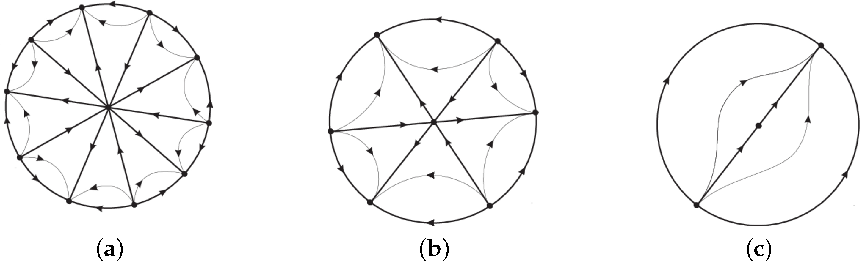
6. Proof of Theorem 1 for $\mathit{n}=\mathbf{4}$

In this section, we are interested in studying the quartic homogeneous Hamiltonian systems with finitely many equilibria given by

$$\begin{array}{c}\dot{x}=-b{x}^4-2c{x}^{3}y-3d{x}^2{y}^2-4ex{y}^3-5f{y}^4,\hfill \\ \dot{y}=5a{x}^4+4b{x}^{3}y+3c{x}^2{y}^2+2dx{y}^3+e{y}^4,\hfill \end{array}$$

(12)

where a, b, c, d, e and f are real parameters. Its corresponding Hamiltonian function is

$H_5(x,y)=a{x}^5+b{x}^{4}y+c{x}^3{y}^2+d{x}^2{y}^3+ex{y}^4+f{y}^5.$

The infinite singularities of this system (12) are determined by the real linear factors of $x\dot{y}-y\dot{x}=-5H_5(x,y)$ that can have twelve different kinds of linear factors. We shall see that only the three cases I, II, III, and IV of system (12) have finitely many equilibria, and the remaining cases have infinitely many singular points.

• If $H_5(x,y)$ has five simple real linear factors $(x-r_{1}y)(x-r_{2}y)(x-r_{3}y)(x-r_{4}y)(x-r_{5}y)$, with $r_1<r_2<r_3<r_4<r_5$, so $H_5(x,y)=a(x-r_{1}y)(x-r_{2}y)(x-r_{3}y)(x-r_{4}y)(x-r_{5}y)$, and system (12) becomes

  $$\begin{array}{cc}\dot{x}=\hfill & r_1+r_2+r_3+r_4+r_5)x^4+2x^{3}y(-r_1{r}_2-r_1{r}_3-r_1{r}_4-r_1{r}_5-r_2{r}_3\hfill \\ \hfill & -r_2{r}_4-r_2{r}_5-r_3{r}_4-r_3{r}_5-r_4{r}_5)+3x^2{y}^2(r_1{r}_2{r}_3+r_1{r}_2{r}_4+r_1{r}_2{r}_5\hfill \\ \hfill & +r_1{r}_3{r}_4+r_1{r}_3{r}_5+r_1{r}_4{r}_5+r_2{r}_3{r}_4+r_2{r}_3{r}_5+r_2{r}_4{r}_5+r_3{r}_4{r}_5)\hfill \\ \hfill & +4x{y}^3(-r_1{r}_2{r}_3{r}_4-r_1{r}_2{r}_3{r}_5-r_1{r}_2{r}_4{r}_5-r_1{r}_3{r}_4{r}_5-r_2{r}_3{r}_4{r}_5)\hfill \\ \hfill & +5r_1{r}_2{r}_3{r}_4{r}_5{y}^4,\hfill \\ \dot{y}=\hfill & -4x^{3}y(r_1+r_2+r_3+r_4+r_5)+3x^2{y}^2(r_1{r}_2+r_1{r}_3+r_1{r}_4+r_1{r}_5\hfill \\ \hfill & +r_2{r}_3+r_2{r}_4+r_2{r}_5-r_3{r}_4+r_3{r}_5+r_4{r}_5)-2x{y}^3(r_1{r}_2{r}_3+r_1{r}_2{r}_4\hfill \\ \hfill & +r_1{r}_2{r}_5+r_1{r}_3{r}_4+r_1{r}_3{r}_5+r_1{r}_4{r}_5+r_2{r}_3{r}_4+r_2{r}_3{r}_5+r_2{r}_4{r}_5+r_3{r}_4{r}_5)\hfill \\ \hfill & -y^4(-r_1{r}_2{r}_3{r}_4-r_1{r}_2{r}_3{r}_5-r_1{r}_2{r}_4{r}_5-r_1{r}_3{r}_4{r}_5-r_2{r}_3{r}_4{r}_5)+5x^4,\hfill \end{array}$$

  (13)
  This system has one finite singularity at the origin of coordinates. In the chart $U_1$ system (13) writes

  $$\begin{array}{cc}\dot{u}=\hfill & -5(r_{1}u-1)(r_{2}u-1)(r_{3}u-1)(r_{4}u-1)(r_{5}u-1),\hfill \\ \dot{v}=\hfill & -(r_1+r_2+r_3+r_4+r_5)v+(2r_1{r}_2+2r_1{r}_3+2r_2{r}_3+2r_1{r}_4+2r_2{r}_4+2r_3{r}_4\hfill \\ \hfill & +2r_1{r}_5+2r_2{r}_5+2r_3{r}_5+2r_4{r}_5)uv+(-3r_1{r}_2{r}_3-3r_1{r}_2{r}_4-3r_1{r}_3{r}_4\hfill \\ \hfill & -3r_2{r}_3{r}_4-3r_1{r}_2{r}_5-3r_1{r}_3{r}_5-3r_2{r}_3{r}_5-3r_1{r}_4{r}_5-3r_2{r}_4{r}_5-3r_3{r}_4{r}_5)u^{2}v\hfill \\ \hfill & +(4r_1{r}_2{r}_3{r}_4+4r_1{r}_2{r}_3{r}_5+4r_1{r}_2{r}_4{r}_5+4r_1{r}_3{r}_4{r}_5+4r_2{r}_3{r}_4{r}_5)u^{3}v-5r_1{r}_2{r}_3{r}_4{r}_5{u}^{4}v.\hfill \end{array}$$
  It is easy to check that this system has five hyperbolic nodes at $(1/r_1,0)$, $(1/r_2,0)$, $(1/r_3,0)$, $(1/r_4,0)$ and $(1/r_5,0)$ with alternative kind of stability. See its phase portrait in Figure 4a.
• If $H_5(x,y)$ has three simple linear factors $(x-r_{1}y)(x-r_{2}y)(x-r_{3}y)$, with $r_1<r_2<r_3$ and two complex linear factors $(x^2-2\alpha \beta xy+({\alpha }^2+{\beta }^2)y^2)$, so

  $$H_5(x,y)=a(x-r_{1}y)(x-r_{2}y)(x-r_{3}y)(x^2-2\alpha \beta xy+({\alpha }^2+{\beta }^2)y^2).$$
  System (12) becomes

  $$\begin{array}{cc}\dot{x}=\hfill & x^4(2\alpha +r_1+r_2+r_3)+2x^{3}y(-{\alpha }^2-{\beta }^2-2\alpha r_1-r_1{r}_2-r_1{r}_3\hfill \\ \hfill & -2\alpha r_2-r_2{r}_3-2\alpha r_3)+3x^2{y}^2({\alpha }^2{r}_1+{\beta }^2{r}_1+2\alpha r_1{r}_2+r_1{r}_2{r}_3\hfill \\ \hfill & +2\alpha r_1{r}_3+{\alpha }^2{r}_2+{\beta }^2{r}_2+2\alpha r_2{r}_3+{\alpha }^2{r}_3+{\beta }^2{r}_3)-4x{y}^3({\alpha }^2{r}_1{r}_2\hfill \\ \hfill & +{\beta }^2{r}_1{r}_2+2\alpha r_1{r}_2{r}_3+{\alpha }^2{r}_1{r}_3+{\beta }^2{r}_1{r}_3+{\alpha }^2{r}_2{r}_3+{\beta }^2{r}_2{r}_3)+5y^4\hfill \\ \hfill & \left({\alpha }^2{r}_1{r}_2{r}_3+{\beta }^2{r}_1{r}_2{r}_3\right),\hfill \\ \dot{y}=\hfill & -4x^{3}y(2\alpha +r_1+r_2+r_3)+3x^2{y}^2({\alpha }^2+{\beta }^2+2\alpha r_1+r_1{r}_2+r_1{r}_3+2\alpha r_2\hfill \\ \hfill & +r_2{r}_3+2\alpha r_3)-2x{y}^3({\alpha }^2{r}_1+{\beta }^2{r}_1+2\alpha r_1{r}_2+r_1{r}_2{r}_3+2\alpha r_1{r}_3+{\alpha }^2{r}_2\hfill \\ \hfill & +{\beta }^2{r}_2+2\alpha r_2{r}_3+{\alpha }^2{r}_3+{\beta }^2{r}_3)-y^4({\alpha }^2(-r_1)r_2-{\beta }^2{r}_1{r}_2-2\alpha r_1{r}_2{r}_3\hfill \\ \hfill & -{\alpha }^2{r}_1{r}_3-{\beta }^2{r}_1{r}_3-{\alpha }^2{r}_2{r}_3\hfill \\ \hfill & -{\beta }^2{r}_2{r}_3)+5x^4.\hfill \end{array}$$

  (14)
  System (14) has one finite singularity at the origin of coordinates. In the chart $U_1$ system (14) written as

  $$\begin{array}{cc}\dot{u}=\hfill & -5(r_{1}u-1)(r_{2}u-1)(r_{3}u-1)\left({\alpha }^2{u}^2+{\beta }^2{u}^2-2\alpha u+1\right),\hfill \\ \dot{v}=\hfill & 2\alpha +5r_1{r}_2{r}_3{u}^4\left({\alpha }^2+{\beta }^2\right)-4u^3({\alpha }^2{r}_1{r}_2+{\beta }^2{r}_1{r}_2+2\alpha r_1{r}_2{r}_3+{\alpha }^2{r}_1{r}_3\hfill \\ \hfill & +{\beta }^2{r}_1{r}_3+{\alpha }^2{r}_2{r}_3+{\beta }^2{r}_2{r}_3)+3u^2({\alpha }^2{r}_1+{\beta }^2{r}_1+2\alpha r_1{r}_2+r_1{r}_2{r}_3+2\alpha r_1{r}_3\hfill \\ \hfill & +{\alpha }^2{r}_2+{\beta }^2{r}_2+2\alpha r_2{r}_3+{\alpha }^2{r}_3+{\beta }^2{r}_3)-2u({\alpha }^2+{\beta }^2+2\alpha r_1+r_1{r}_2+r_1{r}_3\hfill \\ \hfill & +2\alpha r_2+r_2{r}_3+2\alpha r_3)+r_1+r_2+r_3.\hfill \end{array}$$
  We can easily verify that this system has three hyperbolic nodes at $(1/r_1,0)$, $(1/r_2,0)$ and $(1/r_3,0)$ with alternative kind of stability. Consequently its phase portrait is given in Figure 4b.
• If $H_5(x,y)$ has one simple real linear factor $(x-r_{1}y)$ and four complex factors $(x^2-2{\alpha }_{1}xy+y^2({\alpha }_1^2+{\beta }_1^2))(x^2-2{\alpha }_{2}xy+y^2({\alpha }_2^2+{\beta }_2^2))$, so $H_5(x,y)=a(x-r_{1}y)(x^2-2{\alpha }_{1}xy+y^2({\alpha }_1^2+{\beta }_1^2))(x^2-2{\alpha }_{2}xy+y^2({\alpha }_2^2+{\beta }_2^2))$, and system (12) becomes

  $$\begin{array}{cc}\dot{x}=\hfill & -a(x-r_{1}y)(2y({\alpha }_1^2+{\beta }_1^2)-2{\alpha }_{1}x)({(x-{\alpha }_{2}y)}^2+{\beta }_2^2{y}^2)-(x-r_{1}y)\hfill \\ \hfill & ({(x-{\alpha }_{1}y)}^2+{\beta }_1^2{y}^2)(2y({\alpha }_2^2+{\beta }_2^2)-2{\alpha }_{2}x)+r_1({(x-{\alpha }_{1}y)}^2+{\beta }_1^2{y}^2)\hfill \\ \hfill & ({(x-{\alpha }_{2}y)}^2+{\beta }_2^2{y}^2)),\hfill \\ \dot{y}=\hfill & a(2(x-r_{1}y)(x-{\alpha }_{2}y)(x^2-2{\alpha }_{1}xy+y^2({\alpha }_1^2+{\beta }_1^2))+2(x-r_{1}y)\hfill \\ \hfill & (x-{\alpha }_{1}y)(x^2-2{\alpha }_{2}xy+y^2({\alpha }_2^2+{\beta }_2^2))+(x^2-2{\alpha }_{1}xy+y^2({\alpha }_1^2+{\beta }_1^2))\hfill \\ \hfill & (x^2-2{\alpha }_{2}xy+y^2({\alpha }_2^2+{\beta }_2^2))).\hfill \end{array}$$

  (15)
  This system has one finite singularity at the origin of coordinates. In the chart $U_1$ system (15) has one infinite hyperbolic node at $(1/r_1,0)$. So its phase portrait is given in Figure 4c.
• If $H_5(x,y)$ has one simple real linear factor $(x-r_{1}y)$ and double complex linear factors ${(x^2-2\alpha xy+y^2({\alpha }^2+{\beta }^2))}^2$, so $H_5(x,y)=(x-r_{1}y){(x^2-2\alpha xy+y^2({\alpha }^2+{\beta }^2))}^2$, and its corresponding Hamiltonian system also has the phase portrait given in Figure 4c.
  In the following cases of the Hamiltonian $H_5(x,y)$ the corresponding Hamiltonian system has infinitely many singular points, and we do not consider them.
• $H_5(x,y)$ has one double real linear factor and three simple real linear factors.
• $H_5(x,y)$ has two double real linear factors and one simple real linear factor.
• $H_5(x,y)$ has one triple real linear factor and two simple real linear factors.
• $H_5(x,y)$ has one triple real linear factor and one double real linear factor.
• $H_5(x,y)$ has one real linear factor of multiplicity four and one simple real linear factor.
• $H_5(x,y)$ has one real linear factor of multiplicity five.
• $H_5(x,y)$ has one double real linear factor, one simple real linear factor and two complex linear factors.
• $H_5(x,y)$ has one triple real linear factor and two complex linear factors.

This completes the proof of Theorem 1 for $n=4$.

7. Proof of Theorem 1 for $\mathit{n}=\mathbf{5}$

In this section, we are interested in studying the quintic homogeneous Hamiltonian systems with finitely many equilibria given by

$$\begin{array}{c}\dot{x}=-b{x}^5-2c{x}^{4}y-3d{x}^3{y}^2-4e{x}^2{y}^3-5fx{y}^4-6g{y}^5,\hfill \\ \dot{y}=6a{x}^5+5b{x}^{4}y+4c{x}^3{y}^2+3d{x}^2{y}^3+2ex{y}^4+f{y}^5,\hfill \end{array}$$

(16)

where a, b, c, d, e, f and g are real parameters. Its corresponding Hamiltonian function is

$H_6(x,y)=a{x}^6+b{x}^{5}y+c{x}^4{y}^2+d{x}^3{y}^3+e{x}^2{y}^4+fx{y}^5+g{y}^6.$

The infinite singularities of this system (16) are determined by the real linear factors of $x\dot{y}-y\dot{x}=-6H_6(x,y)$ that can have sixteen different kinds of linear factors. Where we shall see that only the four cases I, II, III and IV system (16) have finitely many equilibria, and the remaining cases have infinitely many singular points.

• If $H_6(x,y)$ has six simple non zero real linear factors $(x-r_{1}y)(x-r_{2}y)(x-r_{3}y)(x-r_{4}y)(x-r_{5}y)(x-r_{6}y)$, with $r_1<r_2<r_3<r_4<r_5<r_6$, so $H_6(x,y)=a(x-r_{1}y)(x-r_{2}y)(x-r_{3}y)(x-r_{4}y)(x-r_{5}y)(x-r_{6}y)$, and system (16) becomes

  $$\begin{array}{cc}\dot{x}=\hfill & x^5(r_1+r_2+r_3+r_4+r_5+r_6)+2x^{4}y(-r_1{r}_2-r_1{r}_3-r_1{r}_4\hfill \\ \hfill & -r_1{r}_5-r_1{r}_6-r_2{r}_3-r_2{r}_4-r_2{r}_5-r_2{r}_6-r_3{r}_4-r_3{r}_5-r_3{r}_6\hfill \\ \hfill & -r_4{r}_5-r_4{r}_6-r_5{r}_6)+3x^3{y}^2(r_1{r}_2{r}_3+r_1{r}_2{r}_4+r_1{r}_2{r}_5+r_1{r}_2{r}_6\hfill \\ \hfill & +r_1{r}_3{r}_4+r_1{r}_3{r}_5+r_1{r}_3{r}_6+r_1{r}_4{r}_5+r_1{r}_4{r}_6+r_1{r}_5{r}_6+r_2{r}_3{r}_4\hfill \\ \hfill & +r_2{r}_3{r}_5+r_2{r}_3{r}_6+r_2{r}_4{r}_5+r_2{r}_4{r}_6+r_2{r}_5{r}_6+r_3{r}_4{r}_5+r_3{r}_4{r}_6\hfill \\ \hfill & +r_3{r}_5{r}_6+r_4{r}_5{r}_6)+4x^2{y}^3(-r_1{r}_2{r}_3{r}_4-r_1{r}_2{r}_3{r}_5-r_1{r}_2{r}_3{r}_6\hfill \\ \hfill & -r_1{r}_2{r}_4{r}_5-r_1{r}_2{r}_4{r}_6-r_1{r}_2{r}_5{r}_6-r_1{r}_3{r}_4{r}_5-r_1{r}_3{r}_4{r}_6-r_1{r}_3{r}_5{r}_6\hfill \\ \hfill & -r_1{r}_4{r}_5{r}_6-r_2{r}_3{r}_4{r}_5-r_2{r}_3{r}_4{r}_6-r_2{r}_3{r}_5{r}_6-r_2{r}_4{r}_5{r}_6-r_3{r}_4{r}_5{r}_6)\hfill \\ \hfill & +5x{y}^4(r_1{r}_2{r}_3{r}_4{r}_5+r_1{r}_2{r}_3{r}_4{r}_6+r_1{r}_2{r}_3{r}_5{r}_6+r_1{r}_2{r}_4{r}_5{r}_6\hfill \\ \hfill & +r_1{r}_3{r}_4{r}_5{r}_6+r_2{r}_3{r}_4{r}_5{r}_6)-6r_1{r}_2{r}_3{r}_4{r}_5{r}_6{y}^5,\hfill \\ \dot{y}=\hfill & -5x^{4}y(r_1+r_2+r_3+r_4+r_5+r_6)-4x^3{y}^2(-r_1{r}_2-r_1{r}_3-r_1{r}_4\hfill \\ \hfill & -r_1{r}_5-r_1{r}_6-r_2{r}_3-r_2{r}_4-r_2{r}_5-r_2{r}_6-r_3{r}_4-r_3{r}_5-r_3{r}_6-r_4{r}_5\hfill \\ \hfill & -r_4{r}_6-r_5{r}_6)-3x^2{y}^3(r_1{r}_2{r}_3+r_1{r}_2{r}_4+r_1{r}_2{r}_5+r_1{r}_2{r}_6+r_1{r}_3{r}_4\hfill \\ \hfill & +r_1{r}_3{r}_5+r_1{r}_3{r}_6+r_1{r}_4{r}_5+r_1{r}_4{r}_6+r_1{r}_5{r}_6+r_2{r}_3{r}_4+r_2{r}_3{r}_5\hfill \\ \hfill & +r_2{r}_3{r}_6+r_2{r}_4{r}_5+r_2{r}_4{r}_6+r_2{r}_5{r}_6+r_3{r}_4{r}_5+r_3{r}_4{r}_6+r_3{r}_5{r}_6\hfill \\ \hfill & +r_4{r}_5{r}_6)-2x{y}^4(-r_1{r}_2{r}_3{r}_4-r_1{r}_2{r}_3{r}_5-r_1{r}_2{r}_3{r}_6-r_1{r}_2{r}_4{r}_5\hfill \\ \hfill & -r_1{r}_2{r}_4{r}_6-r_1{r}_2{r}_5{r}_6-r_1{r}_3{r}_4{r}_5-r_1{r}_3{r}_4{r}_6-r_1{r}_3{r}_5{r}_6-r_1{r}_4{r}_5{r}_6\hfill \\ \hfill & -r_2{r}_3{r}_4{r}_5-r_2{r}_3{r}_4{r}_6-r_2{r}_3{r}_5{r}_6-r_2{r}_4{r}_5{r}_6-r_3{r}_4{r}_5{r}_6)\hfill \\ \hfill & -y^5(r_1{r}_2{r}_3{r}_4{r}_5+r_1{r}_2{r}_3{r}_4{r}_6+r_1{r}_2{r}_3{r}_5{r}_6+r_1{r}_2{r}_4{r}_5{r}_6+r_1{r}_3{r}_4{r}_5{r}_6\hfill \\ \hfill & +r_2{r}_3{r}_4{r}_5{r}_6)+6x^5.\hfill \end{array}$$

  (17)
  This system has one finite singularity at the origin of coordinates. In the chart $U_1$ system (17) writes

  $$\begin{array}{cc}\dot{u}=\hfill & 6(r_{1}u-1)(r_{2}u-1)(r_{3}u-1)(r_{4}u-1)(r_{5}u-1)(r_{6}u-1),\hfill \\ \dot{v}=\hfill & v(6r_1{r}_2{r}_3{r}_4{r}_5{r}_6{u}^5-5u^4(r_1{r}_2{r}_3{r}_4{r}_5+r_1{r}_2{r}_3{r}_4{r}_6+r_1{r}_2{r}_3{r}_5{r}_6+r_1{r}_2{r}_4{r}_5{r}_6\hfill \\ & +r_1{r}_3{r}_4{r}_5{r}_6+r_2{r}_3{r}_4{r}_5{r}_6)+4u^3(r_1{r}_2{r}_3{r}_4+r_1{r}_2{r}_3{r}_5+r_1{r}_2{r}_3{r}_6+r_1{r}_2{r}_4{r}_5\hfill \\ & +r_1{r}_2{r}_4{r}_6+r_1{r}_2{r}_5{r}_6+r_1{r}_3{r}_4{r}_5+r_1{r}_3{r}_4{r}_6+r_1{r}_3{r}_5{r}_6+r_1{r}_4{r}_5{r}_6+r_2{r}_3{r}_4{r}_5\hfill \\ & +r_2{r}_3{r}_4{r}_6+r_2{r}_3{r}_5{r}_6+r_2{r}_4{r}_5{r}_6+r_3{r}_4{r}_5{r}_6)-3u^2(r_1{r}_2{r}_3+r_1{r}_2{r}_4+r_1{r}_2{r}_5\hfill \\ & +r_1{r}_2{r}_6+r_1{r}_3{r}_4+r_1{r}_3{r}_5+r_1{r}_3{r}_6+r_1{r}_4{r}_5+r_1{r}_4{r}_6+r_1{r}_5{r}_6+r_2{r}_3{r}_4+r_2{r}_3{r}_5\hfill \\ & +r_2{r}_3{r}_6+r_2{r}_4{r}_5+r_2{r}_4{r}_6+r_2{r}_5{r}_6+r_3{r}_4{r}_5+r_3{r}_4{r}_6+r_3{r}_5{r}_6+r_4{r}_5{r}_6)\hfill \\ & +2u(r_1{r}_2+r_1{r}_3+r_1{r}_4+r_1{r}_5+r_1{r}_6+r_2{r}_3+r_2{r}_4+r_2{r}_5+r_2{r}_6+r_3{r}_4\hfill \\ & +r_3{r}_5+r_3{r}_6+r_4{r}_5+r_4{r}_6+r_5{r}_6)-r_1-r_2-r_3-r_4-r_5-r_6).\hfill \end{array}$$
  It is easy to check that this system has six hyperbolic nodes at $(1/r_1,0)$, $(1/r_2,0)$, $(1/r_3,0)$, $(1/r_4,0)$, $(1/r_5,0)$ and $(1/r_6,0)$ with alternative kind of stability. Then its phase portrait is given in Figure 5a.
• If $H_6(x,y)$ has four simple real linear factors $(x-r_{1}y)(x-r_{2}y)(x-r_{3}y)(x-r_{4}y)$, with $r_1<r_2<r_3<r_4$ and two complex $(x^2-2\alpha xy+y^2({\alpha }^2+{\beta }^2))$, so $H_6(x,y)=a(x-r_{1}y)(x-r_{2}y)(x-r_{3}y)(x-r_{4}y)(x^2-2\alpha xy+y^2\left({\alpha }^2+{\beta }^2\right))$, and system (16) becomes

  $$\begin{array}{cc}\dot{x}=\hfill & x^5(2\alpha +r_1+r_2+r_3+r_4)+2x^{4}y(-{\alpha }^2-{\beta }^2-2\alpha r_1-r_1{r}_2\hfill \\ \hfill & -r_1{r}_3-r_1{r}_4-2\alpha r_2-r_2{r}_3-r_2{r}_4-2\alpha r_3-r_3{r}_4-2\alpha r_4)+3x^3{y}^2\hfill \\ \hfill & ({\alpha }^2{r}_1+{\beta }^2{r}_1+2\alpha r_1{r}_2+r_1{r}_2{r}_3+r_1{r}_2{r}_4+2\alpha r_1{r}_3+r_1{r}_3{r}_4+2\alpha r_1{r}_4\hfill \\ \hfill & +{\alpha }^2{r}_2+{\beta }^2{r}_2+2\alpha r_2{r}_3+r_2{r}_3{r}_4+2\alpha r_2{r}_4+{\alpha }^2{r}_3+{\beta }^2{r}_3+2\alpha r_3{r}_4\hfill \\ \hfill & +{\alpha }^2{r}_4+{\beta }^2{r}_4)+4x^2{y}^3(-{\alpha }^2{r}_1{r}_2-{\beta }^2{r}_1{r}_2-2\alpha r_1{r}_2{r}_3-r_1{r}_2{r}_3{r}_4\hfill \\ \hfill & -2\alpha r_1{r}_2{r}_4-{\alpha }^2{r}_1{r}_3-{\beta }^2{r}_1{r}_3-2\alpha r_1{r}_3{r}_4-{\alpha }^2{r}_1{r}_4-{\beta }^2{r}_1{r}_4-{\alpha }^2{r}_2{r}_3\hfill \\ \hfill & -{\beta }^2{r}_2{r}_3-2\alpha r_2{r}_3{r}_4-{\alpha }^2{r}_2{r}_4-{\beta }^2{r}_2{r}_4-{\alpha }^2{r}_3{r}_4-{\beta }^2{r}_3{r}_4)+5x{y}^4\hfill \\ \hfill & ({\alpha }^2{r}_1{r}_2{r}_3+{\beta }^2{r}_1{r}_2{r}_3+2\alpha r_1{r}_2{r}_3{r}_4+{\alpha }^2{r}_1{r}_2{r}_4+{\beta }^2{r}_1{r}_2{r}_4\hfill \\ \hfill & +{\alpha }^2{r}_1{r}_3{r}_4+{\beta }^2{r}_1{r}_3{r}_4+{\alpha }^2{r}_2{r}_3{r}_4+{\beta }^2{r}_2{r}_3{r}_4)+6y^5({\alpha }^2(-r_1)r_2{r}_3{r}_4\hfill \\ \hfill & -{\beta }^2{r}_1{r}_2{r}_3{r}_4),\hfill \\ \dot{y}=\hfill & -5x^{4}y(r_1+r_2+r_3+r_4+r_5+r_6)-4x^3{y}^2(-r_1{r}_2-r_1{r}_3-r_1{r}_4\hfill \\ & -r_1{r}_5-r_1{r}_6-r_2{r}_3-r_2{r}_4-r_2{r}_5-r_2{r}_6-r_3{r}_4-r_3{r}_5-r_3{r}_6-r_4{r}_5\hfill \\ & -r_4{r}_6)-3x^2{y}^3(r_1{r}_2{r}_3+r_1{r}_2{r}_4+r_1{r}_2{r}_5+r_1{r}_2{r}_6+r_1{r}_3{r}_4+r_1{r}_3{r}_5\hfill \\ & +r_1{r}_3{r}_6+r_1{r}_4{r}_5+r_1{r}_4{r}_6+r_1{r}_5{r}_6+r_2{r}_3{r}_4+r_2{r}_3{r}_5+r_2{r}_3{r}_6+r_2{r}_4{r}_5\hfill \\ & +r_2{r}_4{r}_6+r_2{r}_5{r}_6-r_5{r}_6+r_3{r}_4{r}_5+r_3{r}_4{r}_6+r_3{r}_5{r}_6+r_4{r}_5{r}_6)\hfill \\ & -2x{y}^4(-r_1{r}_2{r}_3{r}_4-r_1{r}_2{r}_3{r}_5-r_1{r}_2{r}_3{r}_6-r_1{r}_2{r}_4{r}_5-r_1{r}_2{r}_4{r}_6-r_1{r}_2{r}_5{r}_6\hfill \\ & -r_1{r}_3{r}_4{r}_5-r_1{r}_3{r}_4{r}_6-r_1{r}_3{r}_5{r}_6-r_1{r}_4{r}_5{r}_6-r_2{r}_3{r}_4{r}_5-r_2{r}_3{r}_4{r}_6\hfill \\ & -r_2{r}_3{r}_5{r}_6-r_2{r}_4{r}_5{r}_6-r_3{r}_4{r}_5{r}_6)-y^5(r_1{r}_2{r}_3{r}_4{r}_5\hfill \\ & +r_1{r}_2{r}_3{r}_4{r}_6+r_1{r}_2{r}_3{r}_5{r}_6+r_1{r}_2{r}_4{r}_5{r}_6+r_1{r}_3{r}_4{r}_5{r}_6+r_2{r}_3{r}_4{r}_5{r}_6)+6x^5.\hfill \end{array}$$

  (18)
  System (18) has one singular point at the origin of coordinates. In the chart $U_1$ system (18) writes

  $$\begin{array}{cc}\dot{u}=\hfill & 6(r_{1}u-1)(r_{2}u-1)(r_{3}u-1)(r_{4}u-1)\left({\alpha }^2{u}^2+{\beta }^2{u}^2-2\alpha u+1\right),\hfill \\ \dot{v}=\hfill & v(-2\alpha +6r_1{r}_2{r}_3{r}_4{u}^5\left({\alpha }^2+{\beta }^2\right)-5u^4({\alpha }^2{r}_1{r}_2{r}_3+{\beta }^2{r}_1{r}_2{r}_3+2\alpha r_1{r}_2{r}_3{r}_4\hfill \\ & +{\alpha }^2{r}_1{r}_2{r}_4+{\beta }^2{r}_1{r}_2{r}_4+{\alpha }^2{r}_1{r}_3{r}_4+{\beta }^2{r}_1{r}_3{r}_4+{\alpha }^2{r}_2{r}_3{r}_4+{\beta }^2{r}_2{r}_3{r}_4)+4u^3({\alpha }^2{r}_1{r}_2\hfill \\ & +{\beta }^2{r}_1{r}_2+{\beta }^2{r}_2{r}_4+r_1{r}_2{r}_3{r}_4+2\alpha r_1{r}_2{r}_4+{\alpha }^2{r}_1{r}_3+{\beta }^2{r}_1{r}_3+2\alpha r_1{r}_3{r}_4+{\alpha }^2{r}_1{r}_4\hfill \\ & +{\beta }^2{r}_1{r}_4+{\alpha }^2{r}_2{r}_3+{\beta }^2{r}_2{r}_3+2\alpha r_2{r}_3{r}_4+{\alpha }^2{r}_2{r}_4+2\alpha r_1{r}_2{r}_3+{\alpha }^2{r}_3{r}_4+{\beta }^2{r}_3{r}_4)\hfill \\ & -3u^2({\alpha }^2{r}_1+{\beta }^2{r}_1+2\alpha r_1{r}_2+r_1{r}_2{r}_3+r_1{r}_2{r}_4+2\alpha r_1{r}_3+r_1{r}_3{r}_4+2\alpha r_1{r}_4+{\alpha }^2{r}_2\hfill \\ & +{\beta }^2{r}_2+2\alpha r_2{r}_3+r_2{r}_3{r}_4+2\alpha r_2{r}_4+{\alpha }^2{r}_3+{\beta }^2{r}_3+2\alpha r_3{r}_4+{\alpha }^2{r}_4+{\beta }^2{r}_4)\hfill \\ & +2u({\alpha }^2+{\beta }^2+2\alpha r_1+r_1{r}_2+r_1{r}_3+r_1{r}_4+2\alpha r_2+r_2{r}_3\hfill \\ & +r_2{r}_4+2\alpha r_3+r_3{r}_4+2\alpha r_4)-r_1-r_1-r_3-r_4).\hfill \end{array}$$
  It is clear that this system has four hyperbolic nodes at $(1/r_1,0)$, $(1/r_2,0)$, $(1/r_3,0)$ and $(1/r_4,0)$ with alternative kind of stability. Its phase portrait is given in Figure 5b.
• If $H_6(x,y)$ has two simple real linear factors $(x-r_{1}y)(x-r_{2}y)$, with $r_1<r_2$ and four complex linear factors $(x^2-2{\alpha }_{1}xy+y^2({\alpha }_1^2+{\beta }_1^2))(x^2-2{\alpha }_{2}xy+y^2({\alpha }_2^2+{\beta }_2^2))$, so $H_6(x,y)=a(x-r_{1}y)(x-r_{2}y)(x^2-2{\alpha }_{1}xy+y^2({\alpha }_1^2+{\beta }_1^2))(x^2-2{\alpha }_{2}xy+y^2({\alpha }_2^2+{\beta }_2^2))$. In this case system (16) becomes

  $$\begin{array}{cc}\dot{x}=\hfill & -a(x-r_{1}y)(x-r_{2}y)(2y({\alpha }_1^2+{\beta }_1^2)-2{\alpha }_{1}x)({(x-{\alpha }_{2}y)}^2+{\beta }_2^2{y}^2)\hfill \\ \hfill & -(x-r_{1}y)(x-r_{2}y)({(x-{\alpha }_{1}y)}^2+{\beta }_1^2{y}^2)(2y({\alpha }_2^2+{\beta }_2^2)-2{\alpha }_{2}x)\hfill \\ \hfill & +r_2(x-r_{1}y)({(x-{\alpha }_{1}y)}^2+{\beta }_1^2{y}^2)({(x-{\alpha }_{2}y)}^2+{\beta }_2^2{y}^2)+r_1(x-r_{2}y)\hfill \\ \hfill & ({(x-{\alpha }_{1}y)}^2+{\beta }_1^2{y}^2)({(x-{\alpha }_{2}y)}^2+{\beta }_2^2{y}^2)),\hfill \\ \dot{y}\hfill & =a(2(x-r_{1}y)(x-r_{2}y)(x-{\alpha }_{2}y)(x^2-2{\alpha }_{1}xy+y^2({\alpha }_1^2+{\beta }_1^2))\hfill \\ & +2(x-r_{1}y)(x-r_{2}y)(x-{\alpha }_{1}y)(x^2-2{\alpha }_{2}xy+y^2({\alpha }_2^2+{\beta }_2^2))\hfill \\ & +(x-r_{1}y)(x^2-2{\alpha }_{1}xy+y^2({\alpha }_1^2+{\beta }_1^2))(x^2-2{\alpha }_{2}xy+y^2({\alpha }_2^2+{\beta }_2^2))\hfill \\ +& \\ & (x-r_{2}y)(x^2-2{\alpha }_{1}xy+y^2({\alpha }_1^2+{\beta }_1^2))(x^2-2{\alpha }_{2}xy+y^2({\alpha }_2^2+{\beta }_2^2))\hfill \end{array}$$

  (19)
  This system has one finite singularity at the origin of coordinates. In the chart $U_1$ system (19) has two hyperbolic nodes at $(1/r_1,0)$ and $(1/r_2,0)$ with an alternative kind of stability. Its phase portrait is given in Figure 5c.
• If $H_6(x,y)$ has two simple real linear factors and two double complex linear factors, in a similar way to III we obtain the phase portrait of Figure 5c.
• If all the linear factors of $H_6(x,y)$ are complex, then its phase portrait is given in Figure 5d.
  In all the other cases different from the cases I to V the homogeneous polynomial $H_6(x,y)$ has at least one double real linear factor and consequently the Hamiltonian system has infinitely many singularities.

In summary Theorem 1 is proved for $n=5$.

8. Conclusions

The main objective of our research revolves around the classification of the phase portraits of five categories of Homogeneous Hamiltonian differential systems of degrees 1, 2, 3, 4, and 5, characterized by a finite number of equilibria. The focus of our study is to present novel results specifically related to the homogeneous Hamiltonian polynomial differential systems with degrees 3, 4, and 5.

References

1. Bautin, N.N. On the number of limit cycles which appear with the variation of coefficients from an equilibrium position of focus or center type. Mat. Sbornik. 1952, 30, 181–196. [Google Scholar]
2. Dulac, H. Détermination et integration d’une certaine classe d’équations différentielle ayant par point singulier un centre. Bull. Sci. Math. Sér. 1908, 32, 230–252. [Google Scholar]
3. Kapteyn, W. On the midpoints of integral curves of differential equations of the first degree. Nederl. Akad. Wetensch. Verslag. Afd. Natuurk. Konikl. Nederland. 1911, 19, 1446–1457. [Google Scholar]
4. Kapteyn, W. New investigations on the midpoints of integrals of differential equations of the first degree. Nederl. Akad. Wetensch. Versl. Afd. Natuurk. 1912, 20, 1354–1365. [Google Scholar]
5. Schlomiuk, D. Algebraic particular integrals, integrability and the problem of the center. Trans. Am. Math. Soc. 1993, 338, 799–841. [Google Scholar] [CrossRef]
6. Vulpe, N.I. Affine invariant conditions for the topological distinction of quadratic systems with a center. Differentsial’nye Uravneniya 1983, 19, 371–379. (In Russian) [Google Scholar]
7. Malkin, K.E. Criteria for the center for a certain differential equation. Volz. Mat. Sb. Vyp. 1964, 2, 87–91. (In Russian) [Google Scholar]
8. Vulpe, N.I.; Sibirskii, K.S. Centro–affine invariant conditions for the existence of a center of a differential system with cubic nonlinearities. Dokl. Akad. Nauk SSSR 1988, 301, 1297–1301. (In Russian) [Google Scholar]
9. Chavarriga, J.; Giné, J. Integrability of a linear center perturbed by a fourth degree homogeneous polynomial. Publ. Mat. 1996, 40, 21–39. [Google Scholar] [CrossRef] [Green Version]
10. Chavarriga, J.; Giné, J. Integrability of a linear center perturbed by a fifth degree homogeneous polynomial. Publ. Mat. 1997, 41, 335–356. [Google Scholar] [CrossRef] [Green Version]
11. Buzzi, C.A.; Llibre, J.; Medrado, J.C. Phase Portraits of reversible linear differential systems with cubic homogeneous polynomial nonlinearities having a non-degenerate center at the origin. Qual. Theory Dyn. Syst. 2009, 7, 369–403. [Google Scholar] [CrossRef]
12. Artés, J.C.; Llibre, J. Quadratic Hamiltonian vector fields. J. Differ. Eq. 1994, 107, 80–95. [Google Scholar] [CrossRef] [Green Version]
13. Dumortier, F.; Llibre, J.; Artés, J.C. Qualitative Theory of Planar Differential Systems; Universitext; Springer: Berlin/Heidelberg, Germany, 2006. [Google Scholar]
14. Neishtadt, A.I.; Sheng, K. Bifurcations of phase portraits of pendulum with vibrating suspension point. Commun. Nonlinear Sci. Numer. Simul. 2017, 47, 71–80. [Google Scholar] [CrossRef] [Green Version]
15. Tian, Y.; Zhao, Y. Global phase portraits and bifurcation diagrams for reversible equivariant Hamiltonian systems of linear plus quartic homogeneous polynomials. Discret. Contin. Dyn. Syst. Ser. B. 2021, 26, 2941–2956. [Google Scholar] [CrossRef]
16. Neumann, L.D.A. Classification of continuous flows on 2–manifolds. Proc. Am. Math. Soc. 1975, 48, 73–81. [Google Scholar] [CrossRef]
17. Markus, L. Structure of ordinary differential equations in the plane. Trans. Am. Math Soc. 1954, 76, 127–148. [Google Scholar] [CrossRef]
18. Peixoto, L.M.M. Dynamical Systems. In Proceedings of the Symposium held at the University of Bahia, Salvador, Brazil, 26 July–14 August 1961; Academic Press: New York, NY, USA, 1973; pp. 389–420. [Google Scholar]
19. Arnold, V.I. Mathematical Methods of Classical Mechanics; Springer: Berlin/Heidelberg, Germany, 1988. [Google Scholar]
Figure 1. Symmetric phase portraits with respect to the origin of coordinates of the homogeneous Hamiltonian systems of degree 1.
Symmetry 15 01476 g001
Figure 3. Symmetric phase portraits with respect to the origin of coordinates of the homogeneous Hamiltonian systems of degree 3.
Symmetry 15 01476 g003
Figure 4. Symmetric phase portraits with respect to the origin of coordinates of the homogeneous Hamiltonian systems of degree 4.
Symmetry 15 01476 g004
Figure 5. Symmetric phase portraits with respect to the origin of coordinates of the homogeneous Hamiltonian systems of degree 5.
Symmetry 15 01476 g005
Disclaimer/Publisher’s Note: The statements, opinions and data contained in all publications are solely those of the individual author(s) and contributor(s) and not of MDPI and/or the editor(s). MDPI and/or the editor(s) disclaim responsibility for any injury to people or property resulting from any ideas, methods, instructions or products referred to in the content.